Inertial-Range Reconnection in Magnetohydrodynamic Turbulence
and in the Solar Wind

Abstract

In situ spacecraft data on the solar wind show events identified as magnetic reconnection with outflows and apparent “$X$-lines” $10^{3-4}$ times ion scales. To understand the role of turbulence at these scales, we make a case study of an inertial-range reconnection event in a magnetohydrodynamic (MHD) simulation. We observe stochastic wandering of field-lines in space, breakdown of standard magnetic flux-freezing due to Richardson dispersion, and a broadened reconnection zone containing many current sheets. The coarse-grain magnetic geometry is like large-scale reconnection in the solar wind, however, with a hyperbolic flux-tube or “X-line” extending over integral length-scales.

Magnetic reconnection is widely theorized to be the source of explosive energy release in diverse astrophysical systems, including solar flares and coronal mass ejections Priest and Forbes (2007), gamma-ray bursts Zhang and Yan (2011), and magnetar giant flares Lyutikov (2006). Because of the large length-scales involved and consequent high Reynolds numbers, many of these phenomena are expected to occur in a turbulent environment, which profoundly alters the nature of reconnection Lazarian and Vishniac (1999); Eyink et al. (2011, 2013). In the solar wind near 1 AU, which is the best-studied turbulent plasma in nature, quasi-stationary reconnection has been observed for magnetic structures at a wide range of scales, from micro-reconnection events at the scale of the ion gyroradius ($\sim$100 km), up to integral length scales ($\sim 10^{4-5}$ km), and even to larger scales Gosling (2012). Yet numerical studies of reconnection in magnetohydrodynamic (MHD) turbulence simulations have focused almost exclusively on small-scale reconnection at the resistive scale Servidio et al. (2010); Zhdankin et al. (2013); Osman et al. (2014). Our objective in this Letter is to identify an inertial-range reconnection event in an MHD turbulence simulation and to determine its characteristic signatures, for comparison with observations in the solar wind and other turbulent astrophysical environments.

To search for reconnection at inertial-range scales we adapt standard observational criteria employed for the solar wind. In pioneering studies, Gosling Gosling (2012) has looked for simultaneous large increments of magnetic field $\delta\mathbf{B}(\mathbf{r})$ and of velocity field $\delta\mathbf{u}(\mathbf{r})$ across space-separations $r$ near the proton gyroradius $\rho_{p}$, which approximate MHD rotational discontinuities. Candidate reconnection events are then identified as pairs of such near-discontinuities, with $\delta\mathbf{B}(\mathbf{r})$ aligned for the two members of the pair and $\delta\mathbf{u}(\mathbf{r})$ anti-aligned. Gosling’s selected events generally have the appearance of two back-to-back shocks, or a “bifurcated current sheet”. We modify this criterion to allow for more gradual field-reversals, by choosing instead $r=L/10,$ with $L$ the outer (integral) length of the turbulent inertial range and by considering pairs separated by distances up to $L/2.$

We apply the above criterion to two datasets. The first is from a numerical simulation of incompressible, resistive MHD in a $[-\pi,\pi]^{3}$ periodic cube, in a state of stationary turbulence driven by a large-scale body-force. The simulation has about a decade of power-law inertial-range and the full output for a large-scale eddy turnover time is archived in an online, web-accessible database Johns Hopkins Turbulence Databases . The second dataset consists of Wind spacecraft observations of the solar wind magnetic field $\mathbf{B}$, velocity $\mathbf{u}$, and proton number density $n_{p}$. The results presented here are from a week-long fast stream in days 14-21 of 2008 (cf. Gosling (2007)). The average solar wind conditions were $u=638$ km/s, $B=4.3$ nT, $n_{p}=2.3$ ${\rm cm}^{-3}$, Alfvén speed $V_{A}=62$ km/s, proton beta $\beta_{p}=1.1,$ and proton gyroradius $\rho_{p}=154$ km. The temporal data-stream from the spacecraft is converted to an equivalent space series using Taylor’s hypothesis, $x=ut$ Taylor (1938). Simulated “spacecraft observations” from the MHD database are taken along 192 linear cuts, with $4^{3}$ cuts through each face of the simulation cube in the three coordinate directions. We find a good correspondence for statistics of $\delta\mathbf{B}(\mathbf{r})$ and $\delta\mathbf{u}(\mathbf{r})$ in the two datasets, with the grid spacing $dx=2\pi/1024$ of the simulation related to $18$ s of the Wind time-series See Supplemental Material for 3D figures, movies and additional documentation of the procedures . We thus estimate the turbulent outer scale $L$ of the solar wind stream to be 6.5$\times 10^{5}$ km, or $\sim$1026 s in time units, compared with $L=0.35$ in the MHD simulation.

Increments $\delta\mathbf{B}(\mathbf{r}),\delta\mathbf{u}(\mathbf{r})$ are considered to be “large” for our criterion when their magnitudes both exceed 1.5 of their rms values. Using this threshold, we identify possible reconnection events in both datasets. See complete catalogues in See Supplemental Material for 3D figures, movies and additional documentation of the procedures . Many of the candidate events in both datasets resemble the “double-step” magnetic reversals bounded by near-discontinuities, which Gosling tends to select with his original criteria Gosling (2012). However, we also see events with more gradual reversals over inertial-range scales in both datasets. In Fig. 1 we show

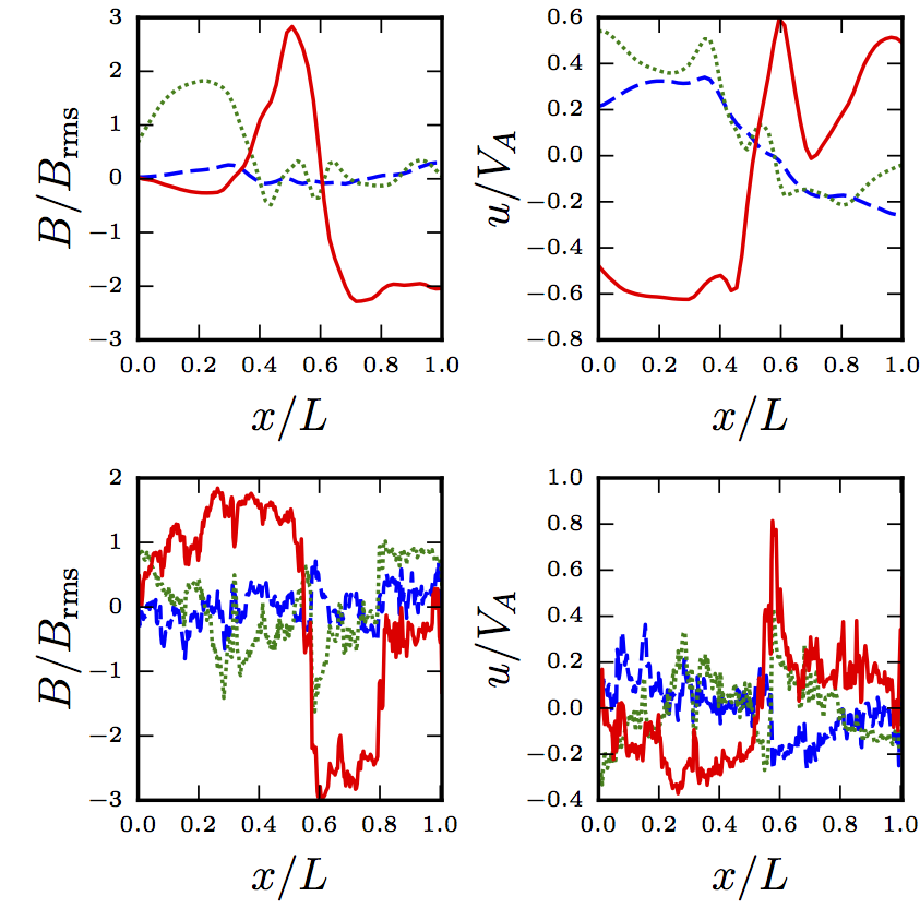
Figure 1: Top: Event from the MHD simulation, at point (2.964,0.908,5.841) along a cut in the $y$-direction. Magnetic fields (left) normalized by $B_{rms}=0.24,$ and velocity fields (right) by local upstream Alfven velocity $V_{A}=0.7$. Bottom: Event from Wind spacecraft data, on January 14, 2008, 13:50 hr, normalized by $B_{rms}=2.5$ nT, $V_{A}=75$ km/s. Distance $x$ is normalized by $L.$ MVF components are identified as L (red, solid), M( green, dotted), N (blue, dashed).

events of this latter type. The vectors have been rotated into the minimum-variance-frame (MVF) of the magnetic field Sonnerup and Cahill (1967), calculated over the reversal region. The velocities here (and in all following plots) are in a frame moving with the local mean plasma velocity. Both events are inertial-range scale, occupying an interval of length 0.1 in the MHD simulation and 2-3 min in the solar wind case. Although they do not have a “double-step” magnetic structure, these two events do show the features characteristic of magnetic reconnection. There appears to be a reconnecting field component and an associated Alfvénic outflow jet in the $L$-direction of maximum variance. A weak inflow is seen in the $N$-direction of minimum variance, which is usually interpreted as across the reconnection “current sheet.” The $M$-direction of intermediate variance is nominally the guide-field direction, which in both events appears rather weak and variable.

The MHD event shown in Fig. 1, top panels, arises from passage of the sampled 1D cut close to a large, helical magnetic flux-rope appearing in the simulation. The maximum field strength in the rope is 8 times the rms strength in the database. Plotted in Fig. 3 is the original 1D spatial cut, the magnetic cloud, and nominally incoming and outgoing field-lines along the N- and L-directions of the MVF. There is a clear magnetic reversal, with incoming lines in the flux-rope twisting clockwise and into the page, but incoming lines to the left pointing out of the page. The field-line geometry is, however, quite complex since the lines exhibit the stochastic wandering assumed in the Lazarian-Vishniac

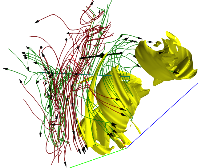
Figure 2: B-isosurface at half-maximum value 1.11 in yellow. $\bf{\mathbf{B}}$-lines sampled along N-direction in green and L-directions in red. The original 1D spatial cut is the thick black line.

theory of turbulent reconnection Lazarian and Vishniac (1999). Fig. 2 and all other spatial plots in this letter are available as 3D PDF’s See Supplemental Material for 3D figures, movies and additional documentation of the procedures .

To identify large-scale geometry, it is necessary to spatially coarse-grain (low-pass filter) the magnetic field. For the theoretical basis of this coarse-graining approach to turbulent reconnection, see Eyink and Aluie (2006); Eyink (2014). Here we apply a box-filter with half-width $L$ to obtain coarse-grained fields $\bar{\mathbf{B}}$, $\bar{\mathbf{u}},$ from which all inertial- and dissipation-range eddies are eliminated. The nature of the database event as large-scale reconnection becomes more evident in Fig. 3, which plots the lines of $\bar{\mathbf{B}}.$ A central “X-point” at (2.84, 1.31, 5.73) was located by eye and a new MVF calculated in a sphere of radius $L$ around that point. (This frame is rotated by $\sim 20^{\circ}$ in all three directions relative to the MVF for the original 1D cut, but furthermore the $M$- and $N$-directions are exchanged). Field-lines are plotted at regular intervals along the $L$- and $N$-axes through the point. The plasma flow is incoming along the $N$-direction and outgoing along the $L$-direction, and the magnetic structure is clearly X-type, with length $\sim$ 0.4-0.6 ($L$-direction) and width $\sim$ 0.15-0.2 ($N$-direction). Reconnection events observed in the solar wind also appear to be X-type Gosling (2012), although this structure has generally been interpreted in terms of Petschek reconnection.

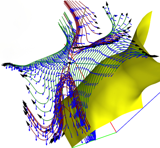
Figure 3: Same as Fig. 2, except for $\bar{\mathbf{B}}$ rather than $\mathbf{B}.$ The isosurface is for the half-maximum value $|\bar{\mathbf{B}}|=0.301$. The blue vectors on the field-lines are $\bar{\mathbf{u}}$ (in the local plasma frame).

In fact, the field-line geometry of $\bar{\mathbf{B}}$ in the MHD event is more complex than a single “X-point.” The complete structure is revealed by calculating the “perpendicular squashing factor” $Q_{\perp},$ a quantity devised to identify field-lines with rapidly changing connectivity in the solar photosphere and corona Titov (2007). We consider the $Q_{\perp}$-factor for the field-lines of $\bar{\mathbf{B}}$ which begin and end on a sphere of radius 1.6$L$ around the nominal “X-point” in Fig. 3. The $Q_{\perp}$-isosurface in Fig. 4 reveals a “quasi-separatrix layer” (QSL) whose cross-section has a clear $X$-type structure. The “hyperbolic flux-tube” (HFT) extending along the centers of these $X$’s has length about 0.54 and is aligned approximately with the $M$-direction, to within about $35^{\circ}.$ An HFT is the modern version of an “X-line” for 3D reconnection, which does not usually admit true separatrices and X-lines, and an HFT has the same observational consequences as an X-line. It is thus interesting that very large-scale reconnection events in the solar wind (above integral scales) appear to have very extended $X$-lines, based on observations by multiple spacecraft Phan et al. (2009).

Careful examination of the dynamics of this MHD event verifies that it is indeed magnetic reconnection, and fundamentally influenced by turbulence. The magnetic flux-rope and the associated QSL persist over the entire time (0 to 2.56) of the database, drifting slowly with the plasma. The QSL and MVF also slowly rotate in time, with the MVF directions rotated through total angles $\sim 40^{\circ}$ at the final time and also the $M$- and $N$-directions exchanged around time $2.0.$ The time required for a plasma fluid element in the reconnection region to be carried out by the exhausts with velocities $\sim 0.3$-$0.4$ also happens to be about 2.0. Despite the high conductivity of the simulation, standard flux-freezing is violated in this event due to the turbulent phenomenon of “spontaneous stochasticity”, as we now verify. The exact stochastic flux-freezing theorem for resistive MHD Eyink (2009) (which generalizes ordinary flux-freezing), states that field-lines of the fine-grained magnetic field $\mathbf{B}$ are “frozen-in” to the stochastic trajectories solving the Langevin equation

$$d\mathbf{x}/dt=\mathbf{u}(\mathbf{x},t)+\sqrt{2\lambda}\ d\hbox{\boldmath$\eta$}(t),$$ (1)

where $\lambda=\eta c^{2}/4\pi$ is magnetic diffusivity and $\hbox{\boldmath$\eta$}(t)$ is a 3D Gaussian white-noise. The many “virtual” field-vectors $\tilde{\mathbf{B}}$ which arrive to the same final point must be averaged to obtain the physical magnetic field $\mathbf{B}$ at that point. We have chosen a point $\mathbf{x}_{f}$ in the outflow jet in the $+L$-dir-

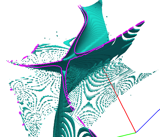
Figure 4: The quasi-separatrix layer $Q_{\perp}=32$ in cyan, and its cross-section in a plane normal to the $M$-direction in magenta.

ection at time $t_{f}=2$ and solved (1) backward in time to $t_{0}=0,$ to find the positions of the initial points whose magnetic field vectors arrive at $(\mathbf{x}_{f},t_{f}).$ This ensemble of points, plotted in Fig. 5, is widely dispersed in space. This disagrees with the predictions of standard flux-freezing, which implies that the ensemble should be close to a single point. In the lower panel of Fig. 5 is plotted the mean-square dispersion of this ensemble perpendicular to the L-direction, $\langle r_{\perp}^{2}\rangle$ as a function of reversed time $\tau=t_{f}-t.$ Consistent with previous results Eyink et al. (2013), the (backward) growth of perpendicular dispersion is diffusive $\langle r_{\perp}^{2}(\tau)\rangle\sim 8\lambda\tau$ for very small $\tau$ but then becomes super-ballistic, due to turbulent Richardson dispersion. As argued in Eyink et al. (2011), the perpendicular spread in the time to exit with the outflow, $\sqrt{\langle r_{\perp}^{2}(2)\rangle}\sim 0.19,$ is close to the width of the reconnection region. This zone has both the width and the turbulent structure proposed in Lazarian and Vishniac (1999), as can be seen also in Fig. 5 which plots in green the isosurfaces of the fine-grained current magnitude at half-maximum. There is a spatial distribution of many current sheets rather than a single large current sheet, as in laminar reconnection, and none of the sheets is located precisely at the QSL shown in Fig. 4. See See Supplemental Material for 3D figures, movies and additional documentation of the procedures for 3D plots.

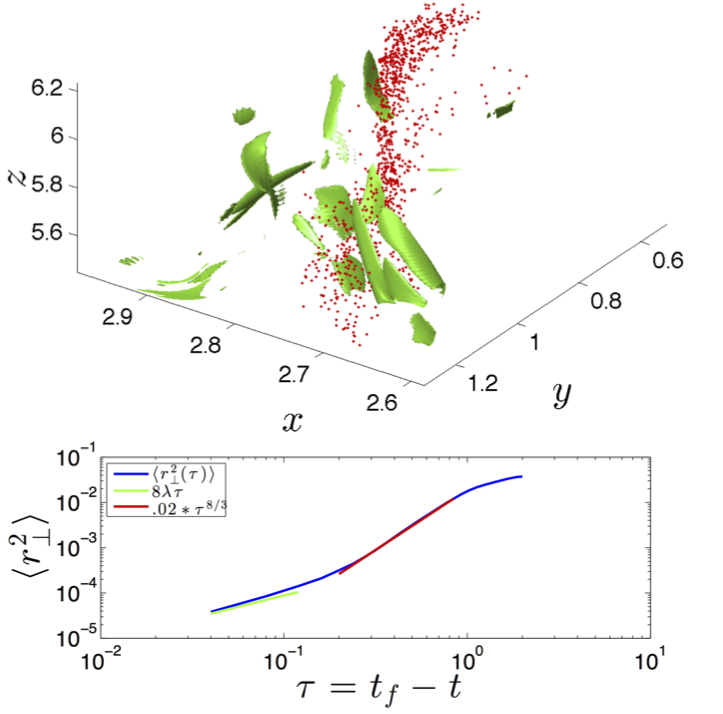
Figure 5: Top: Vorticity isosurfaces at the half-maximum value $\omega=69.1$ in green. In red, origin points at time $t=0$ of magnetic field at final point $(\mathbf{x}_{f},t_{f})=(3.31,0.083,6.07,2.00)$. Bottom: Backward mean-square dispersion $\langle r_{\perp}^{2}(\tau)\rangle$ orthogonal to $L$-direction as blue line. Reference curve $\langle r_{\perp}^{2}\rangle=8\lambda\tau$ in green, and $\langle r_{\perp}^{2}\rangle=0.02\tau^{8/3}$ in red.

The breakdown of standard flux-freezing is one evidence of reconnection in this event Greene (1993). We have also verified that there is topology change of the lines of both fine-grained and coarse-grained magnetic fields. To show this, we decorate initial field-lines of either $\mathbf{B}$ or $\bar{\mathbf{B}}$ at time $t=0$ with a sequence of plasma fluid elements and then follow each element moving with the local velocity $\mathbf{u}$ forward in time to $t=2.$ We find that the plasma elements which initially resided on the same line at $t=0$ end up on distinct lines at time $t=2$ and some of these lines are outgoing in the $+L$-direction and others in the $-L$-direction. For movies, see See Supplemental Material for 3D figures, movies and additional documentation of the procedures . We have also determined the average reconnecting electric field $E_{{\rm rec}}$ for the large-scale magnetic field $\bar{\mathbf{B}},$ using a voltage measure proposed in Kowal et al. (2009). We find that $E_{{\rm rec}}\sim 0.01v_{A}B$ in terms of local upstream values $v_{A}$ and $B$. Furthermore, at the length scale $L$ of $\bar{\mathbf{B}},$ most of $E_{{\rm rec}}$ is supplied by turbulence-induced electric fields and resistivity gives only a tiny contribution, always more than an order of magnitude smaller. These and many other detailed results for this event will be presented elsewhere. One finding is that this inertial-range event is not only highly 3D but also non-stationary in time. While the outflow jets are quite stable over time, the inflow is “gusty”, with variable magnitude and direction veering in the $N$-$M$-plane (so that it is often in the nominal guide-field or $M$-direction). It is thus difficult to define an operationally meaningful “reconnection speed”.

The main purpose of this Letter has been to present an example of inertial-range reconnection in MHD turbulence, to clarify its observational signatures. While a fluid description is surely applicable only to scales much larger than plasma micro-scales (e.g. the ion gyroradius in the collisionless solar wind), our simulation is remarkably successful in reproducing observed features of large-scale solar-wind reconnection, together with crucial turbulent effects supporting theoretical predictions in Lazarian and Vishniac (1999); Eyink et al. (2011). The characteristics are expected to change with length-scale, e.g. reconnection deeper within the inertial-range should have stronger guide-fields/smaller magnetic shear-angles Lazarian and Vishniac (1999); Gosling et al. (2007). We also note some differences between the current MHD database and the solar wind, as our simulation is incompressible and isothermal, whereas the solar wind is slightly compressible and reconnection events there (including that in Fig. 1) often show enhancements of proton density and temperature in the reconnection zone. Furthermore, our MHD simulation has no mean magnetic field and is close to balance between Alfvén waves propagating parallel and anti-parallel to field-lines, whereas the solar wind has a moderate mean field and the high-speed stream studied in this work is dominated by Alfvén waves propagating outward from the sun. The influence of these differences should be explored in future work seeking to explain large-scale solar wind reconnection in detail within an MHD turbulence framework.

.1 Acknowledgments

This work was supported by NSF grants CDI-II: CMMI 0941530 and AST 1212096.

References

- Priest and Forbes (2007) E. Priest and T. Forbes, Magnetic Reconnection: MHD Theory and Applications (Cambridge University Press, 2007).
- Zhang and Yan (2011) B. Zhang and H. Yan, Astrophys. J. 726, 90 (2011).
- Lyutikov (2006) M. Lyutikov, Mon. Not. Roy. Astr. Soc. 367, 1594 (2006).
- Lazarian and Vishniac (1999) A. Lazarian and E. Vishniac, Astrophys. J. 517, 700 (1999).
- Eyink et al. (2011) G. L. Eyink, A. L. Lazarian, and E. T. Vishniac, Astrophys. J. 743, 51 (2011).
- Eyink et al. (2013) G. Eyink, E. Vishniac, C. Lalescu, H. Aluie, K. Kanov, K. Bürger, R. Burns, C. Meneveau, and A. Szalay, Nature 497, 466 (2013).
- Gosling (2012) J. T. Gosling, Space. Sci. Rev. 172, 187 (2012).
- Servidio et al. (2010) S. Servidio, W. H. Matthaeus, M. A. Shay, P. Dmitruk, P. A. Cassak, and M. Wan, Physics of Plasmas 17, 032315 (2010).
- Zhdankin et al. (2013) V. Zhdankin, D. A. Uzdensky, J. C. Perez, and S. Boldyrev, Astrophys. J. 771, 124 (2013).
- Osman et al. (2014) K. T. Osman, W. H. Matthaeus, J. T. Gosling, A. Greco, S. Servidio, B. Hnat, S. C. Chapman, and T. D. Phan, Phys. Rev. Lett. 112, 215002 (2014).
- (11) Johns Hopkins Turbulence Databases, http://turbulence.pha.jhu.edu.
- Gosling (2007) J. T. Gosling, Astrophys. J. Lett. 671, L73 (2007).
- Taylor (1938) G. I. Taylor, Roy. Soc. Lond. Proc. Ser. A 164, 476 (1938).
- (14) See Supplemental Material for 3D figures, movies and additional documentation of the procedures, http://link.aps.org/supplemental/??????/PhysRevLett.??????
- Sonnerup and Cahill (1967) B. U. O. Sonnerup and L. J. Cahill, Jr., J. Geophys. Res. 72, 171 (1967).
- Eyink and Aluie (2006) G. L. Eyink and H. Aluie, Physica D 223, 82 (2006).
- Eyink (2014) G. L. Eyink, ArXiv e-prints (2014), arXiv:1412.2254 [astro-ph.SR] .
- Titov (2007) V. S. Titov, Astrophys. J. 660, 863 (2007).
- Phan et al. (2009) T. D. Phan, J. T. Gosling, and M. S. Davis, Geophys. Res. Lett. 36, L09108 (2009).
- Eyink (2009) G. L. Eyink, J. Math. Phys. 50, 083102 (2009).
- Greene (1993) J. M. Greene, Phys. Fluids B 5, 2355 (1993).
- Kowal et al. (2009) G. Kowal, A. Lazarian, E. T. Vishniac, and K. Otmianowska-Mazur, Astrophys. J 700, 63 (2009).
- Gosling et al. (2007) J. T. Gosling, T. D. Phan, R. P. Lin, and A. Szabo, Geophys. Res. Lett. 34, L15110 (2007).