TIED LINKS

Abstract.

In this paper we introduce the tied links, i.e. ordinary links provided with some ‘ties’ between strands. The motivation for introducing such objects originates from a diagrammatical interpretation of the defining generators of the so–called algebra of braids and ties; indeed, one half of such generators can be interpreted as the usual generators of the braid algebra, and the other half can be interpreted as ties between consecutive strands; this interpretation leads to the definition of tied braids. We define an invariant polynomial for the tied links via a skein relation. Furthermore, we introduce the monoid of tied braids and we prove the corresponding theorems of Alexander and Markov for tied links. Finally, we prove that the invariant of tied links we defined can be obtained also by using the Jones recipe.

Introduction

Since the seminal works of Jones [9] on the famous invariants for classical links, now called the Jones polynomial, several other classes of knotted objects have been proposed, singular links [4, 6, 17], framed links [13] and virtual knots [12], among others. This paper introduces and studies a new class of knotted objects, the tied links. Tied links are the closure of tied braids; tied braids come from a diagrammatical interpretation of the defining generators of the so–called algebra of braids and ties, in short bt–algebra, which appeared the first time in [10] and [1] and was studied in different contexts in [16], [5] and [2]. The bt–algebra was firstly introduced as a tool to study the representation theory of the Vassiliev algebra (see [1, Section 2.1]) and consequently to construct new representations of the braid group. Also, in [1] it is shown that this algebra can be Yang–baxterized in the sense of Jones.

Let $n$ be a positive integer, the bt–algebra ${\mathcal{E}}_{n}$ is a 1–parameter unital associative algebra, defined through a presentation with generators $T_{1},\ldots,T_{n-1}$ and $E_{1},\ldots,E_{n-1}$ and certain relations, for details see Definition 8. The defining relations of ${\mathcal{E}}_{n}$ make evident that the generators $T_{i}$’s can be interpreted diagrammatically as the usual braids generators. On the contrary, an immediate diagrammatical interpretation of the generators $E_{i}$’s is not evident. However, in [1] we proposed the interpretation of the generator $E_{i}$ as a tie that connects the $i$–strand with the $(i+1)$–strand, thus making the bt–algebra a diagrams algebra. In [2] we have proved that the bt–algebra supports a Markov trace. Consequently, using this Markov trace, the classical theorems of Markov and Alexander for classical links, and certain representation of the classical braid group in the bt–algebra, w e have defined an invariant, at three parameters, for classical links; an analogous route yields an invariant for singular links; see [2] for details. Now, we associate to the bt–algebra the tied braid monoid, which is defined essentially as the monoid having a presentation analogous to the bt–algebra, but taking into account only the monomial relations. We call tied braids the elements of this monoid and tied links the closure of the tied braids. Notice that the classical links can be regarded as tied links since the braid group can be considered naturally as a submonoid of the tied braid monoid.

This paper is largely inspired by our work [2] on the bt–algebra. More precisely, we introduce and study the tied braid monoid and the tied links. In particular, we define an invariant for tied links which ‘contains’ the invariants for classical links defined in [2]. This invariant is defined in two ways: one by a skein relation and the other one by the Jones recipe, that is, via normalization and rescaling of the composition of a representation of the tied braid monoid in the bt–algebra with the Markov trace defined on it.

This paper is organized as follows. In Section 1, we define the tied links, their diagrams and their isotopy classes. In Section 2, we prove the first main result (Theorem 1) of the paper, that is, the construction, via skein relation, of an invariant polynomial for tied links, which we shall denote $\mathcal{F}$. The proof of the existence of such invariant is an adaptation of the proof given in [14] for the Homflypt polynomial for classical knots. Further, we provide the value of the invariant on simple examples of tied links. Section 3, is devoted to the understanding of the tied links through the introduction of a new object, that we call the monoid of tied braids (Definition 6); also, in this section we prove the analogous of the Alexander theorem (Theorem 2) and of the Markov theorem (Theorem 3) for tied links. Section 4, has as goal the construction of the invariant $\mathcal{F}$ through the Jones recipe, i.e., by the composition of the natural representation of the monoid of tied braids in the bt–algebra with the trace on the bt–algebra defined in [2, Theorem 3]; this construction is done in Theorem 5. Finally, Section 5 is devoted to the computer algorithm to obtain the value of $\mathcal{F}$ for any tied link put in the form of a closed tied braid; the algorithm calculates the trace of the tied braid and then the polynomial for the tied link via the Jones recipe.

It is a pleasure to dedicate this work to the memory of Slavik Jablan, who since 2010 showed interest in our algorithm to calculate the invariant (for classical links) ${\mathcal{F}}$, here presented, and whose existence was at that time only conjectured. We will always be grateful to Slavik, in particular for his personal way of being a mathematician as an authentic ‘truth lover’. Slavik always enjoyed sharing his knowledge and achievements with extreme generosity.

1. Tied links

In this section we introduce the concepts of tied links and of their diagrams. In fact, a tied link is a link whose set of components is subdivided into classes. Our Definitions 1 and 3 are motivated by the concept of a tie as a notational device to indicate that two components of a link belong to the same class. The tie is an arc drawn from a point on one component to a point on the other or the same component. It will be indicated by a wavy line and it is part of the formalism that the way this arc is embedded in three–space is not relevant.

Definition 1.

A tied (oriented) link $L(P)$ with $n$ components is a set $L$ of $n$ disjoint smooth (oriented) closed curves embedded in $S^{3}$, and a set $P$ of ties, i.e., unordered pairs of points $(p_{r},p_{s})$ of such curves between which there is an arc called a tie. Ties are depicted as springs connecting pairs of points lying on the curves. The tie is a notational device, not an embedded arc. Arcs can cross through it. We shall denote $\mathcal{T}$ the set of oriented tied links.

Remark 1.

If $P$ is the empty set, the tied link $L(P)$ is nothing else but the classical link $L$.

Definition 2.

A tied link diagram is like the diagram of a link, provided with ties, depicted as springs connecting pairs of points lying on the curves.

Observe that the set $P$ defines a partition of the set of the components of $L$ into classes in this way: if a tie connects two components, then these components belong to the same class. Observe also that the sets of components of two isotopic links are equal, and can be identified.

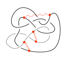
Figure 1. The diagram of a tied link.

Definition 3.

Two oriented tied links $L(P)$ and $L^{\prime}(P^{\prime})$ are tie–isotopic if:

1. the links $L$ and $L^{\prime}$ are ambient isotopic

2. The sets $P$ and $P^{\prime}$ define the same partition of the set of components of $L$ and $L^{\prime}$.

In other words the tie–isotopy says that, when remaining in the same equivalence class, it is allowed to move any tie between two components letting its extremes move along the two whole components. Moreover, ties can be destroyed or created between two components, provided that these components either coincide, or belong to the same class.

Definition 4.

Two components will be said tied together, if they belong to the same class, i.e., if between them a tie already exists or a tie can be created.

Examples of diagrams of tie isotopic tied links are given in Figure 2. The links have three components D, G and B (respectively for Dark, Green and Blue). The three links are evidently ambient isotopic. The three components are all tied together, i.e., they belong to a sole class. Indeed, in the first two diagrams D is tied with G and with B. Therefore G results to be tied with B. A tie between G and B is in fact present in the third diagram. Other ties can be destroyed, i.e., the tie between D and itself in the first two diagrams, the tie between G and itself in the first diagram, and the second tie between D and G the second diagram.

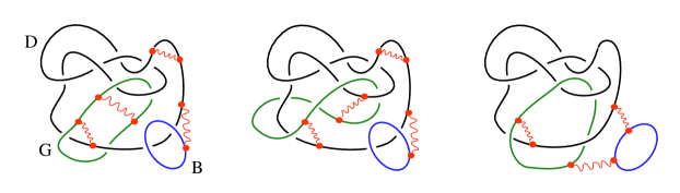
Figure 2. Diagrams of tie–isotopic tied links.

Since the Reidemeister moves preserve the link components, it is evident that the diagrams of two tie–isotopic links can be transformed one into the other by means of the usual Reidemeister moves: the extremes of the ties can be always shifted, so that the ties result to be outside the ball into which each move takes place. Remember that the ties can freely move (provided only that the endpoints move continuously on the curves), overstepping other ties as well as the link curves.

Definition 5.

We call essential a tie between two components, if it cannot be destroyed (i.e. by removing it, the components become untied). Therefore, an essential tie always exists between distinct components.

Remark 2.

A tied link with $n$ components is therefore nothing else but a link where the components are colored with $m\leq n$ distinct colors [3]; two components have the same color if they are tied together. However, we deal with diagrams that are made by links with ties, and that may look arbitrarily complicated.

2. An invariant for tied links

In order to define our invariant for tied links, we need to fix some notations. From now on we fix three indeterminates $u$, $z$ and $w$, and we set $A={\mathbb{C}}(u,z,w)$.

Let us denote by $\mathcal{T}$ the set of oriented tied links diagrams. Notice that an invariant of tied links is a function from $\mathcal{T}$ in $A$ that takes one constant value on each class of tie–isotopic links.

Notation. In the sequel, if there is no risk of confusion, we indicate by $TL$ both the oriented tied link and its diagram.

2.1.

The following theorem is a counterpart of the theorem stated in [14, page 112] for classical links.

Theorem 1.

There exists a function $\mathcal{F}:\mathcal{T}\rightarrow A$, invariant of oriented tied links, uniquely defined by the following three conditions on tied–links diagrams:

• The value of $\mathcal{F}$ is equal to 1 on the unknotted circle (no matter if tied with itself)

• Let $TL$ be a tied link. By $TL^{o}$ we denote the tied link consisting of $TL$ and the unknotted circle (no matter if tied with itself), unlinked to $TL$. Then

  $$\mathcal{F}(TL^{o})=\frac{1}{wz}\mathcal{F}(TL)$$

• Skein rule: let $TL_{+},TL_{-},TL_{\sim},TL_{+,\sim}$ be the diagrams of tied links, that are identical outside a small disc into which enter two strands, whereas inside the disc the two strands look as shown in Fig. 3. Then the following identity holds:

  $$\frac{1}{w}\mathcal{F}(TL_{+})-w\mathcal{F}(TL_{-})=\left(1-u^{-1}\right)\mathcal{F}(TL_{\sim})+\frac{1}{w}(1-u^{-1})\mathcal{F}(TL_{+,\sim}).$$

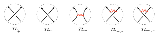
Figure 3. The discs, where $TL_{+},TL_{-}$, $TL_{\sim}$ and $TL_{+,\sim}$ are not tie-isotopic.

Remark 3.

The following three skein rules, all equivalent to the skein rule above, will be used in the sequel. The first one is obtained from III, simply adding a tie between the two strands inside the disc. The rules Va,b follow from III and IV.

1. $$\frac{1}{uw}\mathcal{F}(TL_{+,\sim})-w\mathcal{F}(TL_{-,\sim})=(1-u^{-1})\mathcal{F}(TL_{\sim})$$

2. $$\frac{1}{w}\mathcal{F}(TL_{+})=w\left[\mathcal{F}(TL_{-})+\left({u}-1\right)\mathcal{F}(TL_{-,\sim})\right]+\left(u-1\right)\mathcal{F}(TL_{\sim})$$

3. $$w\mathcal{F}(TL_{-})=\frac{1}{w}[\mathcal{F}(TL_{+})+(u^{-1}-1)\mathcal{F}(TL_{+,\sim})]+({u^{-1}}-1)\mathcal{F}(TL_{\sim}).$$

Proof.

Theorem 1 is proved by the same procedure used in [14]. We will outline the parts where the presence of ties modifies the demonstration.

According to [14], the fact that the skein rules, together with the value of the invariant on the unknotted circle, are sufficient to define the value of the invariant on any tied link is proved as follows.

Let $\mathcal{T}^{n}$ be the set of diagrams of tied links with $n$ crossings, and $TL\in\mathcal{T}^{n}$. Ordering the components and fixing a point in each component, for every diagram $TL$ an associated standard ascending diagram $TL^{\prime}$ is constructed. This ascending diagram is obtained by starting at the base point of the first component of $TL$, and proceeding along that component, changing the overpasses to underpasses (where necessary) so that every crossing is first encountered as an underpass. Continue from the base point of the second and of all subsequent components in the same way. This process separates and unknots the components. The diagrams $TL$ and $TL^{\prime}$ are thus identical except for a finite number of crossings, here called ‘deciding’, where the signs are opposite. Furthermore, we define here $\widetilde{TL}^{\prime}$, adding to $TL^{\prime}$ a tie between the strands near to each dec iding crossing. $TL^{\prime}$ and $\widetilde{TL}^{\prime}$ are by construction collections of unknotted and unlinked components; $TL^{\prime}$ has the same ties as $TL$, $\widetilde{TL}^{\prime}$ may have more ties. The procedure defining $TL^{\prime}$ allows us to get an ordered sequence of deciding crossings, whose order depends on the ordering of the components, and on the choice of the base points.

The induction hypothesis states that we have a function $\mathcal{F}:\mathcal{T}^{n}\rightarrow A$, which satisfies relations I–III. This function is independent of the ordering of the components, independent of the choices of the base points, and invariant under Reidemeister moves which do not increase the number of crossings beyond $n$. Moreover, also by induction hypothesis, the value of $\mathcal{F}$ on any diagram with $n$ crossings of the tied link $TL_{0}^{c,m}$, consisting of $c$ components unknotted and untied, connected by $m$ essential ties ($m\leq c-1$), is equal to $t^{m}/(wz)^{c-1}$, where

(1) $$t:=\frac{z(uw^{2}-1)}{(1-u)}$$

(observe that these values of $\mathcal{F}$ are independent of $n$).

One starts with zero crossings: the tied link is thus a collection of $c\geq 1$ curves unknotted and unlinked, with $m\leq c-1$ essential ties between them. The value of $\mathcal{F}$ on such tied link is given by $t^{m}/(wz)^{c-1}$.

Now, let $TL$ be in $\mathcal{T}^{n+1}$. If $TL$ consists of $c$ components unknotted and untied, connected by $m$ essential ties ($m\leq c-1$), then we define

(2) $$\mathcal{F}(TL)=\frac{t^{m}}{(wz)^{c-1}}.$$

Otherwise, consider the first deciding crossing $P$. If in a neighborhood of $P$ the tied link looks like $TL_{+,\sim}$ (or $TL_{-,\sim}$), then we use skein rule IV to write the value of $\mathcal{F}$ in terms of $TL_{-,\sim}$ and $TL_{\sim}$ (respectively, $TL_{+,\sim}$ and $TL_{\sim}$). If in a neighborhood of $P$ the tied link looks like $TL_{+}$ (respectively, $TL_{-}$), then we use skein rule V-a (resp., V-b) to write the value of $\mathcal{F}$ in terms of the value of $\mathcal{F}$ on the tied links $TL_{-},TL_{-,\sim}$ and $TL_{\sim}$ (respectively, $TL_{+},TL_{+,\sim}$ and $TL_{\sim}$). Observe that if the tied links $TL_{\sigma}$ or $TL_{\sigma,\sim}$ ($\sigma=\pm$) coincide with the original tied link in a neighborhood of the crossing $P$, then $TL_{-\sigma}$ and $TL_{-\sigma,\sim}$ in the neighborhood of the same crossing coincide with the associated tied link $TL^{\prime}$ or $\widetilde{TL}^{\prime}$. On the other hand, $TL_{\sim}$ represents a tied link diagram with $n$ crossings, for which the value of $\mathcal{F}$ i s known, and invariant according to the induction hypothesis. Then we apply the same procedure to the second deciding crossing, which is present in all the diagrams, obtained by the application of the skein rules, and that results to have $n+1$ crossings, and so on. The procedure ends with the last deciding crossing, thus obtaining unlinked and unknotted tied links, with $n+1$ crossings, where the value of $\mathcal{F}$ is given by (2), depending only on the number of components and the number of essential ties.

Observe that the skein rule IV could be avoided: this should extend the procedure.

It remains to prove that:

1. the procedure is independent from the order of the deciding points

2. the procedure is independent from the order of components, and from the choice of base–points

3. the function is invariant under Reidemeister moves.

Following the proof done in [14] for classical links, we observe that the proofs of points ($i$), ($ii$), and ($iii$) can also be done in an analogous way in presence of ties. Of course, every time a skein rule is used, we have to pay attention to all tied links involved (the skein relation for $\mathcal{F}$ involves four tied links diagrams, whereas the skein relation for the classical Homflypt polynomial involves only three). We write here the proof of statement ($i$) as an example. The proofs of the other statements are similar.

The proof of statement (i) consists in a verification that the value of the invariant does not change if we interchange any two deciding points in the procedure of calculation. So, let $TL$ be the diagram of a tied link and let $p$ and $q$ the first two deciding crossings that will be interchanged.

Denote by $\epsilon_{p}$ the sign at the crossing $p$, by $\sigma_{p}TL$ the tied link obtained from $TL$ by changing the sign at the crossing $p$, by $\tilde{\sigma}_{p}TL$ the tied link obtained by $TL$ changing the sign at $p$ and adding a tie near $p$, and by $\rho_{p}TL$ the tied link obtained by $TL$ removing the crossing $p$ and adding a tie. Then, do the same for point $q$.

If $q$ follows $p$, then, by skein relations Va,b,

$$\mathcal{F}(TL)=w^{2\epsilon_{p}}[\mathcal{F}(\sigma_{p}TL)+(u^{\epsilon_{p}}-1)\mathcal{F}(\tilde{\sigma}_{p}TL)]+w^{\epsilon_{p}}(u^{\epsilon_{p}}-1)\mathcal{F}(\rho_{p}TL)$$

and

$$\mathcal{F}(TL) = w^{2\epsilon_{p}}\{w^{2\epsilon_{q}}[\mathcal{F}(\sigma_{q}\sigma_{p}TL)+(u^{\epsilon_{q}}-1)\mathcal{F}(\tilde{\sigma}_{q}\sigma_{p}TL)]+w^{\epsilon_{q}}(u^{\epsilon_{q}}-1)\mathcal{F}(\rho_{q}\sigma_{p}TL)\}$$

$$+(u^{\epsilon_{p}}-1)w^{2\epsilon_{p}}\{w^{2\epsilon_{q}}[\mathcal{F}(\sigma_{q}\tilde{\sigma}_{p}TL)+(u^{\epsilon_{q}}-1)\mathcal{F}(\tilde{\sigma}_{q}\tilde{\sigma}_{p}TL)]+w^{\epsilon_{q}}(u^{\epsilon_{q}}-1)\mathcal{F}(\rho_{q}\tilde{\sigma}_{p}TL)\}$$

$$+(u^{\epsilon_{p}}-1)w^{\epsilon_{p}}\{w^{2\epsilon_{q}}[\mathcal{F}(\sigma_{q}\rho_{p}TL)+(u^{\epsilon_{q}}-1)\mathcal{F}(\widetilde{\sigma}_{q}\rho_{p}TL)]+w^{\epsilon_{q}}(u^{\epsilon_{q}}-1)\mathcal{F}(\rho_{q}\rho_{p}TL)\}.$$

If $p$ follows $q$, then $\mathcal{F}(TL)$ is obtained from the above expression by interchanging $p$ with $q$. Observe that this expression contains terms of type $\mathcal{F}(\tau_{q}\tau_{p}TL)$ or $\alpha(\mathcal{F}(\tau_{p}\tau^{\prime}_{q}TL)+\mathcal{F}(\tau^{\prime}_{p}\tau_{q}TL))$, where $(\tau,\tau^{\prime})\in\{\sigma,\tilde{\sigma},\rho\}$ and $\alpha$ is a coefficient. Such terms are invariant under the interchange of $p$ with $q$, because the operation $\tau_{p}$ commutes with $\tau_{q}$ as well as with $\tau^{\prime}_{q}$. Therefore $\mathcal{F}(TL)$ is independent of the order of $(p,q)$.

∎

Remark 4.

The necessity of II in the definition of $\mathcal{F}$ (Theorem 1) is due to the fact that by the sole skein relation we cannot calculate the value of $\mathcal{F}$ on $c$ unknotted and unlinked circles, without ties between them.

The value $X_{c}$ of $\mathcal{F}$ on $c$ unknotted and unlinked circles, all tied together, can be calculated using skein rule IV recursively $(c-1)$ times, i.e.

$$\frac{1}{uw}X_{c}-wX_{c}=(1-u^{-1})X_{c+1},\quad\quad\text{from which}\quad\quad X_{c+1}=\frac{t}{wz}X_{c}.$$

The initial value $X_{1}=1$ of $\mathcal{F}$ is given by rule I, see Figure 4.

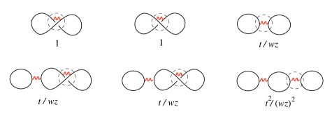
Figure 4. The values of $\mathcal{F}$ on the unknotted and unlinked tied circles involved in skein rule IV.

Remark 5.

Because of Remark 1, we observe that the polynomial $\mathcal{F}$ provides in particular an invariant polynomial for classical links.

2.2. Properties of the Polynomial $\mathcal{F}$

Here we list some properties of the polynomial $\mathcal{F}$, which can be easily verified.

1. $\mathcal{F}$ is multiplicative with respect to the connected sum of tied links

2. The value of $\mathcal{F}$ does not change if the orientations of all curves of the link are reversed

3. Let $TL$ be a link diagram whose components are all tied together, and $TL^{\pm}$ be the link diagram obtained from $TL$ by changing the signs of all crossings. Thus $\mathcal{F}(TL^{\pm})$ is obtained from $\mathcal{F}(TL)$ by the following changes: $w\rightarrow 1/w$ and $u\rightarrow 1/u$

4. Let $\Gamma$ be a knot or a link whose components are all tied together, then $\mathcal{F}(\Gamma)$ is defined by I and IV, and therefore satisfies the following Homflypt–type skein relation, cf. [14]:

   (3) $$\ell\mathcal{F}(TL_{+,\sim})+\ell^{-1}\mathcal{F}(TL_{-,\sim})+m\mathcal{F}(TL_{\sim})=0$$

   where

   $$\ell=\frac{i}{\sqrt{u}w}\quad\text{and}\quad m=i\left(\frac{1}{\sqrt{u}}-\sqrt{u}\right).$$

Item (i) is deduced from the defining relation I of $\mathcal{F}$, and by the same arguments that prove the multiplicativity of the invariants obtained by skein relations (see [14]). Item (ii) is evident, since the value of $\mathcal{F}$ on the unlinked circles is independent of their orientations, and the skein relations are invariant under the inversion of the strands orientations. Item (iii) follows from the fact that, if $w\rightarrow 1/w$ and $u\rightarrow 1/u$, the skein relations Va and Vb are interchanged, whereas the term $t/wz$ remains unchanged.

As for item (iv), observe that if the components of the links are all tied together, or there is a unique component, then adding a tie anywhere does not alter the isotopy class of the link; therefore, in the neighborhood of every crossing, $TL_{+}$ (or $TL_{-}$) can be replaced by $TL_{+,\sim}$ (or $TL_{-,\sim}$), and it can be treated by the sole skein relation IV. Thus, it is evident that there is a bijection between the set of isotopy classes of classical links and the isotopy classes of tied links having all components tied together. In terms of diagrams, it is enough to add (to remove) a tie near every crossing of the diagram of the classical link, as well as a tie between disjoint parts of the diagram (see Figure 5).

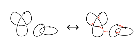
Figure 5. Bijection between classical links and tied links with all components tied together.

Now, multiplying relation IV (Remark 3) by $u^{1/2}$ we obtain the skein relation (3), which is the defining skein relation of the Homflypt polynomial.

Remark 6.

By writing $w$ in terms of the variables $u,z,t$ according to equation (1):

$$w=\sqrt{(z+t-ut)/uz}$$

we observe that the polynomial $\mathcal{F}$ can be always expressed as a Laurent polynomial in the variables $u,z,t$, multiplied for $w^{\epsilon}$, where $\epsilon=1,0,-1$. In order to recover the polynomial $\mathcal{F}$ by means of the Jones recipe, it turns out convenient to express $\mathcal{F}$ in this way.

2.3. Examples

Let $H^{+}$, $H^{-}$, $\widetilde{H^{+}}$, $\widetilde{H^{-}}$, $T^{+}$, $T^{-}$ and $E$ be the tied links shown in Figure 6.

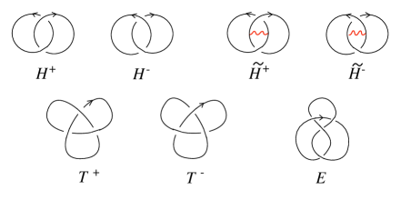
Figure 6.

We show the calculation of $\mathcal{F}$ for the first link $H^{+}$; for the others we write the result of the calculation only.

Using skein rule Va, applied to the upper crossing of $H^{+}$, we write

$$\mathcal{F}(H^{+})=w^{2}(\mathcal{F}(H_{1})+(u-1)\mathcal{F}(H_{2}))+w\mathcal{F}(H_{3})$$

where $H_{1},H_{2},H_{3}$ are shown in the figure below.

We know that, by rules I and II, and by Remark 4:

$$\mathcal{F}(H_{1})=\frac{1}{wz},\quad\quad\mathcal{F}(H_{2})=\frac{t}{wz},\quad\quad\mathcal{F}(H_{3})=1.$$

Therefore,

$$\mathcal{F}(H^{+})=\frac{w}{z}(1+ut+uz-t-z).$$

For the other links of Figure 6, we get:

$$\mathcal{F}(H^{-})=\frac{u^{2}+z+t-uz-ut}{uw(z+t-ut)},$$

$$\mathcal{F}(\widetilde{H^{+}})=\frac{w}{z}(ut+uz-z),\qquad\mathcal{F}(\widetilde{H^{-}})=\frac{u^{2}t+z+t-uz-ut}{uw(z+t-ut)},$$

$$\mathcal{F}(T^{+})=\frac{-u^{3}tz-u^{3}t^{2}+2u^{2}t^{2}+3u^{2}tz+u^{2}z^{2}-3utz-uz^{2}-ut^{2}+tz+z^{2}}{uz^{2}},$$

$$\mathcal{F}(T^{-})=\frac{z(-u^{3}t+u^{2}t-ut+u^{2}z-uz+z+t)}{u(z+t-ut)^{2}},$$

$$\mathcal{F}(E)=\frac{u^{3}t^{2}+u^{3}tz-2u^{2}t^{2}-4u^{2}tz-u^{2}z^{2}+ut^{2}+3uz^{2}+4utz-z^{2}-tz}{uz(z+t-ut)}.$$

Remark 7.

Observe that the last three links are in fact knots (links with one component). For these links, any tie should connect the component with itself, i.e. the tie is not essential.

3. The tied braid monoid

The study of classical links through the braid group is based on the classical theorems of Alexander and Markov. The Alexander theorem states that any link can be obtained by closing a braid. The Markov theorem states when two braids yield isotopic links. These theorems are repeated for singular knots [6, 8], framed knots [13], virtual knots [12] and $p$–adic framed links [11]. That is, in each of these classes of knotted objects, a convenient analogous of the braid group is defined and analogous Alexander and Markov theorems are established. In this section we introduce the monoid of tied braids which plays the role of the braid group for tied links. Thus, we will establish the Alexander theorem and Markov theorem for tied links.

3.1.

We introduce now the monoid of tied braids and we discuss the diagrammatic interpretation for its defining generators.

Definition 6.

The tied braid monoid $T\!B_{n}$ is the monoid generated by usual braids $\sigma_{1},\ldots,\sigma_{n-1}$ and the generators $\eta_{1},\ldots,\eta_{n-1}$, called ties, such the $\sigma_{i}$’s satisfy braid relations among them together with the following relations:

(4) $$\eta_{i}\eta_{j} = \eta_{j}\eta_{i}\qquad\text{ for all $i,j$}$$

(5) $$\eta_{i}\sigma_{i} = \sigma_{i}\eta_{i}\qquad\text{ for all $i$}$$

(6) $$\eta_{i}\sigma_{j} = \sigma_{j}\eta_{i}\qquad\text{for $|i-j|>1$ }$$

(7) $$\eta_{i}\sigma_{j}\sigma_{i} = \sigma_{j}\sigma_{i}\eta_{j}\qquad\text{ for $|i-j|=1$}$$

(8) $$\eta_{i}\sigma_{j}\sigma_{i}^{-1} = \sigma_{j}\sigma_{i}^{-1}\eta_{j}\qquad\text{ for $|i-j|=1$}$$

(9) $$\eta_{i}\eta_{j}\sigma_{i} = \eta_{j}\sigma_{i}\eta_{j}\quad=\quad\sigma_{i}\eta_{i}\eta_{j}\qquad\text{ for $|i-j|=1$}$$

(10) $$\eta_{i}\eta_{i} = \eta_{i}\qquad\text{ for all $i$}.$$

In terms of diagrams the defining generator $\eta_{i}$ corresponds to a tie connecting the $i$ with $(i+1)$–strands and $\sigma_{i}$ is represented as the usual braid diagram:

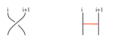
Figure 7. Diagrammatic representation of $\sigma_{i}$ and $\eta_{i}$.

Now we examine the defining relations of $T\!B_{n}$ in terms of these diagrammatic interpretations of the defining generators. Relations (4) and (6) are trivial. Relation (5) corresponds to the sliding of the tie through the crossing. Consider now relations (7) and (8) in terms of diagrams. The first one corresponds to the sliding of the tie from top to bottom behind or in front of a strand. The second one corresponds to the same sliding but bypassing the strand.

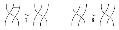
Figure 8. Examples of relations (7) and (8).

Finally, we see relations (9) and (10) in diagrams. Without loss of generality, let us assume $i=2$, $j=1$ in (9), so that

(11) $$\eta_{2}\eta_{1}\sigma_{2}=\eta_{1}\sigma_{2}\eta_{1}=\sigma_{2}\eta_{2}\eta_{1}.$$

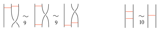
Figure 9. Relations (9) and (10).

3.2. Generalized ties

Now we are going to study certain elements $\eta_{i,j}$ for all $|i-j|>1$. These elements can be defined algebraically as follows,

$$\eta_{i,j}=\sigma_{i}\cdots\sigma_{j-2}\eta_{j-1}\sigma_{j-2}^{-1}\cdots\sigma_{i}^{-1}$$

see after proof of [16, Lemma 1]. In fact, we want to analyze them in terms of diagrams; we will see that, diagrammatically, $\eta_{i,j}$ corresponds to a tie joining the strand $i$ with the strand $j$. Furthermore, this generalized long tie has the property that it is transparent with respect to all strands between the strands $i$ and $j$; i.e it can be drawn no matter if in front or behind these strands. We start by giving a closer look to the following particular elements $\eta_{i,j}$:

(12) $$\eta_{i,i+2}:=\sigma_{i+1}^{-1}\eta_{i}\sigma_{i+1}.$$

We firstly multiply both terms of relation (7) at left by $\sigma_{j}^{-1}$ and at right by $\sigma_{i}^{-1}$, obtaining

(13) $$\sigma_{j}^{-1}\eta_{i}\sigma_{j}=\sigma_{i}\eta_{j}\sigma_{i}^{-1}\qquad|i-j|=1$$

and secondly we multiply both terms of relation (7) at left by $\sigma_{j}^{-1}$ and at right by $\sigma_{j}^{-1}$, obtaining

(14) $$\sigma_{j}^{-1}\eta_{i}\sigma_{j}=\sigma_{i}^{-1}\eta_{j}\sigma_{i}\qquad|i-j|=1.$$

Combining the last two equations we get

(15) $$\eta_{i,j+1}:=\sigma_{j}^{-1}\eta_{i}\sigma_{j}=\sigma_{i}\eta_{j}\sigma_{i}^{-1}=\sigma_{j}^{-1}\eta_{i}\sigma_{j}=\sigma_{i}^{-1}\eta_{j}\sigma_{i}\qquad|i-j|=1.$$

In particular, for $n=3$, equations (15) are expressed, in terms of diagrams, by:

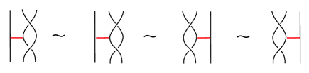
Figure 10. $\eta_{1,3}$ and its equivalent diagrams.

Observe now that, if the ties are provided with elasticity, each one of the elements representing $\eta_{1,3}$ in Figure 10 can be transformed, by a Reidemeister move of second type in which the tie is stretched, in the following compact diagram (i.e., a tie connecting strand 1 with strand 3). From now on, the tie, having elastic property, will be represented as a spring.

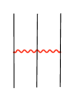
Figure 11. A compact diagram for $\eta_{1,3}$.

Note that it does not matter whether the tie in the compact diagram of Figure 11, is in front or behind the strand 2.

Another advantage of considering the compact diagram (Figure 11) is that the equation:

(16) $$\eta_{i}\sigma_{j}=\sigma_{j}\sigma_{j}^{-1}\eta_{i}\sigma_{j}=\sigma_{j}\eta_{i,j+1}$$

can be interpreted as the sliding of the tie up and down along the braid under stretching or contracting. In other words, while the elements $\eta_{i}$ do not commute with $\sigma_{j}$ for $|j-i|=1$, the equation (16) can be interpreted as a sort of commutation between $\sigma_{i}$ and ties. The situation for $n=3$ is:

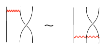
Figure 12. $\eta_{1}\sigma_{2}=\sigma_{2}\eta_{1,3}$.

Let us continue regarding the case $n=3$ . By using equations (16) and (4), we obtain from (11) the following equalities

(17) $$\sigma_{2}\eta_{1,3}\eta_{1}=\eta_{1}\sigma_{2}\eta_{1}=\eta_{1}\eta_{1,3}\sigma_{2}.$$

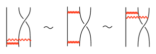
Figure 13. Relations(17).

Comparing now (11) with (17) we get

(18) $$\eta_{1,3}\eta_{1}=\eta_{1}\eta_{1,3}=\eta_{1}\eta_{2}.$$

On the other hand, by using equation (9) we deduce

(19) $$\eta_{1,3}\eta_{2}=\eta_{2}\eta_{1,3}=\eta_{2}\eta_{1}.$$

Having present (4), we have in terms of diagram the following equivalent diagrams:

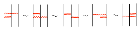
Figure 14. Left: relations (18); right: relations (19).

Hence, in general for $j-i=1$, we have that $\eta_{i,j+1}$ commute with $\eta_{i}$, $\eta_{j}$ and

(20) $$\eta_{i,j+1}\eta_{i}=\eta_{i}\eta_{i,j+1}\eta_{j}=\eta_{i}\eta_{j}.$$

We are now ready to generalize the elements $\eta_{i,j+1}$ ($j-i=1$), to the elements $\eta_{i,k}$, for every $k\geq i$, i.e., $\eta_{i,k}$ will be represented by a spring connecting the strand $i$ with the strand $k$. We shall say also that such tie has length equal to $k-i$.

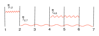
Figure 15. Examples of $\eta_{i,k}$.

Of course, each $\eta_{i}$ is a tie of length 1.

$$\eta_{i,i+1}=\eta_{i}.$$

We define also the tie of zero length, as the monoid unit:

(21) $$\eta_{i,i}=1.$$

In virtue of the tie transparency, there are different expressions of $\eta_{i,k}$ in terms of the $\sigma_{j}$ and $\eta_{j}$. An example is given in Figure 16, where the three diagrams are all equivalent to $\eta_{2,7}$. The proof of the equivalence is based on equations (13) and (14).

There are in fact $(k-i-1)2^{k-i-1}$ equivalent expressions of $\eta_{i,k}$. Let $s_{i}$ denote either the element $\sigma_{i}$ or $\sigma_{i}^{-1}$, and let $\overline{s}_{i}=s_{i}^{-1}$.

Given a pair $i,k$ such that $k-i>1$, the following $2^{k-i-1}$ expressions of $\eta_{i,k}$, obtained for all possible choices of $s_{l}=\sigma_{l}$ or $s_{l}=\sigma_{l}^{-1}$:

$$\eta_{i,k}=s_{i}s_{i+1}s_{i+2}\cdots s_{k-2}\eta_{k-1}\overline{s}_{k-2}\cdots\overline{s}_{i+1}\overline{s}_{i}$$

are all equivalent. Moreover, for every $j$ such that $i\leq j<k-1$ there are similarly $2^{k-i-1}$ equivalent expressions:

$$\eta_{i,k}=s_{i}s_{i+1}\cdots s_{j-1}s_{k-1}s_{k-2}\cdots s_{j+1}\eta_{j}\overline{s}_{j+1}\cdots\overline{s}_{k-1}\overline{s}_{j-1}\dots\overline{s}_{i+1}\overline{s}_{i}.$$

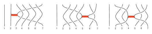
Figure 16. $\sigma_{6}^{-1}\sigma_{5}^{-1}\sigma_{4}^{-1}\sigma_{3}^{-1}\eta_{2}\sigma_{3}\sigma_{4}\sigma_{5}\sigma_{6}\sim\sigma_{2}\sigma_{3}\sigma_{4}\sigma_{6}\eta_{5}\sigma_{6}^{-1}\sigma_{4}^{-1}\sigma_{3}^{-1}\sigma_{2}^{-1}\sim\sigma_{2}^{-1}\sigma_{3}^{-1}\sigma_{6}\sigma_{5}\eta_{4}\sigma_{5}^{-1}\sigma_{6}^{-1}\sigma_{3}\sigma_{2}$.

Similarly, the generalization of (20) to all $\eta_{i,k}$ reads (for $i\leq k\leq m$) (see examples in Figure 17):

(22) $$\eta_{i,k}\eta_{k,m}=\eta_{i,k}\eta_{i,m}=\eta_{k,m}\eta_{i,m}.$$

In particular, if $k=m$, we get

$$\eta_{i,k}\eta_{k,k}=\eta_{i,k}\eta_{i,k}$$

i.e., by (21), all ties $\eta_{i,k}$ are idempotent. This follows as well from any expression of $\eta_{i,k}$, in virtue of (10).

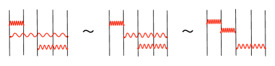
Figure 17. Examples of relation (22): $\eta_{1,2}\eta_{1,5}\eta_{3,5}=\eta_{1,2}\eta_{2,5}\eta_{3,5}=\eta_{1,2}\eta_{2,3}\eta_{3,5}$.

Note also that the definition of $\eta_{i,k}$ for every $k\geq i$ is compatible with the generalization to the case $k\leq i$, by assuming, for every $k\geq i$

(23) $$\eta_{k,i}=\eta_{i,k}.$$

Before concluding this section let us see the generalization of equation (16) to generalized ties of any length.

Let $s=\pm 1$. Observe the identities

(24) $$\sigma_{i}^{s}\eta_{i+1}=\sigma_{i}^{s}\eta_{i+1}(\sigma_{i}^{-s}\sigma_{i}^{s})=(\sigma_{i}^{s}\eta_{i+1}\sigma_{i}^{-s})\sigma_{i}^{s}=\eta_{i,i+2}\sigma_{i}^{s}$$

(25) $$\eta_{i+1}\sigma_{i}^{s}=(\sigma_{i}^{s}\sigma_{i}^{-s})\eta_{i+1}\sigma_{i}^{s}=\sigma_{i}^{s}(\sigma_{i}^{-s}\eta_{i+1}\sigma_{i}^{s})=\sigma_{i}^{s}\eta_{i,i+2}.$$

They can be interpreted as the sliding of the tie up and down along the braid under stretching or contracting. In other words, while the element $\sigma_{i}^{\pm 1}$ does not commute with $\eta_{j}$ when $|j-i|=1$, equations (24) and (25) provide a sort of commutation rule between $\sigma_{i}^{\pm 1}$ and the spring.

Similarly, a spring $\eta_{i,j}$ of any length bigger than one, ‘commutes’  (changing its length by $\pm 1$) with $\sigma_{i}$ and $\sigma_{i-1}$, as well as with $\sigma_{j-1}$ and $\sigma_{j}$, according to the equalities:

$$\eta_{i,j}\sigma_{i}=\sigma_{i}\eta_{i+1,j},\quad\eta_{i,j}\sigma_{i-1}=\sigma_{i-1}\eta_{i-1,j},\quad\eta_{i,j}\sigma_{j}=\sigma_{j}\eta_{i,j+1},\quad\eta_{i,j}\sigma_{j-1}\sigma_{j-1}=\eta_{i,j-1}.$$

The same equalities hold for the inverse of the generators $\sigma_{i}$’s. Therefore, in terms of diagrams, every $\eta_{i,j}$ can be moved to the bottom or to the top of the tied braid. More precisely, we have the following proposition.

Proposition 1 (mobility property).

In any tied braid all ties can be moved to the bottom (or to the top). I.e., any tied braid can be put in the form $\beta\alpha$ (or $\alpha^{\prime}\beta$), where $\beta$ is a usual braid, and $\alpha$ ($\alpha^{\prime}$) is a set of generalized ties.

The generalized ties and its properties allow us to formulate the next propositions which play an important role in the next section.

Proposition 2.

Any set of generalized ties in $T\!B_{n}$ defines an equivalence relation on the set of $n$ strands.

Proof.

The properties of reflectivity, symmetry and transitivity follow directly from equations (21), (23) and (22). ∎

Proposition 3.

Let $B_{1}$ and $B_{2}$ be two tied braids in $T\!B_{n}$. Let us write $B_{1}=\beta_{1}\alpha_{1}$ and $B_{2}=\beta_{2}\alpha_{2}$ according to Proposition 1. Then $B_{1}=B_{2}$ if and only if $\beta_{1}=\beta_{2}$ in $B_{n}$ and $\alpha_{1}$ and $\alpha_{2}$ define the same partition of the set of the strands.

3.3. The Markov and Alexander theorems for tied links

By taking the obvious monomorphism of monoids $T\!B_{n}$ into $T\!B_{n+1}$, we can consider the inductive limit $T\!B_{\infty}$ associated to the inclusions chain $T\!B_{2}\subset\cdots\subset T\!B_{n-1}\subset T\!B_{n}\subset\cdots$. As in the classical case, given a tied braid $\tau$ we denote by $\widehat{\tau}$ its closure, which is a tied link. We have then a map from $T\!B_{\infty}$ to $\mathcal{T}$. We are going to prove now that in fact this map is surjective (Theorem 2). Later, we define the Markov moves for tied braids and then we prove a Markov theorem for tied links (Theorem 3).

Theorem 2 (Alexander theorem for tied links).

Every oriented tied link can be obtained by closing a tied braid.

Proof.

Given a tied link $L(P)$, one fixes a center $O$ in the plane of the diagram of $L(P)$ and proceeds according to the Alexander procedure for classical links. The ties do not prevent the procedure because of their transparency, so that the tied link that we obtain is isotopy equivalent to $L(P)$. However, such a tied link has ties connecting pairs of points in any direction. Using the property that the ends of the ties can slide freely along the strands of the link and that the ties are transparent, we arrange them so that the ends of each tie lie on one half line originating at $O$, not coinciding with the halfline where we open $L(P)$ (see Figure 18). The obtained braid will have horizontal ties connecting two points of different strands. This is by construction a tied braid whose closure is isotopy equivalent to $L(P)$. ∎

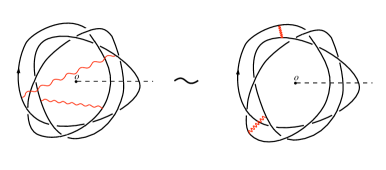
Figure 18. Arranging the ties.

Notation. Let $\beta$ be a tied braid in $TB_{n}$. We denote $s_{\beta}$ the permutation associated, as usual, to the braid obtained from $\beta$ by forgetting the ties in it.

Definition 7.

Two tied braids in the monoid $T\!B_{\infty}$ are $\sim_{T}$–equivalent if one can be obtained from the other by a finite sequence of moves belonging to the following set of operations (or moves):

1. $\alpha\beta$ can be exchanged with $\beta\alpha$

2. $\alpha$ can be exchanged with $\alpha\sigma_{n}$ or $\alpha\sigma_{n}^{-1}$

3. $\alpha$ can be exchanged with $\alpha\eta_{i,j}$ if $s_{\alpha}(i)=j$

for all $\alpha,\beta\in T\!B_{n}$.

Theorem 3 (Markov Theorem for tied links).

Two tied braids have tie–isotopic closures if and only if they are $\sim_{T}$–equivalent.

Proof.

Let $L_{1}$ and $L_{2}$ be two tie–isotopic tied links, and $B_{1}$ and $B_{2}$ the corresponding tied braids whose closures give respectively $L_{1}$ and $L_{2}$, according to Theorem 2. We have to prove that $B_{1}$ and $B_{2}$ are $\sim_{T}$–equivalent. Firstly, as in the case of the Alexander theorem, we can proceed for tied links as in the proof of the Markov theorem for classical links, using the elasticity property, transparency property, and the fact that the ends of the ties can freely slide along the strands. The moves (1) and (2) of Definition 7 coincide in fact with the classical Markov moves; further, observe that the ties do not prevent these moves. By consequence, the braids $\beta_{1}$ and $\beta_{2}$, obtained from $B_{1}$ and $B_{2}$ by forgetting the ties, are Markov–equivalent. Therefore, we can use the Markov moves (1) and (2) to transform $\beta_{1}$ into $\beta_{2}$. In this way, $B_{1}$ and $B_{2}$, after these operations, consist in the same braid $\beta=\beta_{2}$ with $n$ strands, to which ties are added somewhere. Since $L_{1}$ and $L_{2}$ are tie–isotopic, in particular they have the same set $C$ of components. Moreover, the ties of $L_{1}$ and the ties of $L_{2}$ define the same partition of $C$, according to Definition 3. Therefore, the ties of $B_{1}$ and $B_{2}$, under braids closure, define the same partition of $C$. However, in general, the ties in $B_{1}$ do not coincide with those in $B_{2}$. Even worse, by writing $B_{1}=\beta\alpha_{1}$ and $B_{2}=\beta\alpha_{2}$ (see Proposition 1), in general $\alpha_{1}$ and $\alpha_{2}$ do not define the same partition of the set of $n$ strands, i.e., by Proposition 3, $B_{1}\not=B_{2}$. We shall prove that, by using move (3), we can put $B_{1}$ and $B_{2}$ in an equivalent form. Namely, by using repeatedly move (3), we add at the bottom of both $B_{1}$ and $B_{2}$ the element $\gamma$, formed by all the elements $\eta_{i,j}$, for every $i=1,\dots,n$ such that $s_{\beta}(i)=j\not=i$. I.e., we obtain $B_{k}\sim_{T}\beta\alpha_{k}\gamma$, for $k=1,2$ and we must prove that $\beta\alpha_{1}\gamma=\beta\alpha_{2}\gamma$. To do this, it is sufficient, by Proposition 3, to prove that $\alpha_{1}\gamma$ and $\alpha_{2}\gamma$ define the same partition of the set of strands. Now, observe that the cycles of the permutation defined by $\beta$ correspond to the components of the original links. Since $s_{\beta}(i)=j$ if and only if $i$ and $j$ belong to the same cycle, hence $\gamma$ contains $\eta_{i,j}$ if $i$ and $j$ belong to the same component of the links. I.e., every subset in the strands partition defined by $\gamma$ contains strands belonging to a sole links component. Remember that $\alpha_{1}$ and $\alpha_{2}$ contains ties that define, under braid closure, the same partition of the links components. Therefore, both $\alpha_{1}$ and $\alpha_{2}$ do not contain necessarily ties connecting the same component, i.e., pairs of strands contained in a same subset; conversely, if $\alpha_{1}$ contains a tie connecting two strands belonging to two different subsets, then $\alpha_{2}$ must contain a tie connecting two strands belonging to the same two subsets. Therefore, every subset of the partition of the set of strands defined by both $\alpha_{1}\gamma$ and $\alpha_{2}\gamma$ is either a subset, or the union the same subsets defined by $\gamma$. Hence $\alpha_{1}\gamma=\alpha_{2}\gamma$.

∎

4. Construction of $\mathcal{F}$ via the Jones recipe

The procedure to construct the Homflypt polynomial done in [9], leads to a generic way to construct an invariant of knotted objects, which is called Jones recipe. The main objective of this section is to use the Jones recipe to construct the invariant $\mathcal{F}$, see Theorem 5. To do that, we firstly note that Theorems 3 and 2 allow to see the set of tied links as the set of equivalence classes, under $\sim_{T}$, of $T\!B_{\infty}$. Secondly, in Proposition 4 below, we define a representation of the $T\!B_{\infty}$ in the so–called bt–algebra. This representation together with a Markov trace, supported by the bt–algebra, are the main ingredients in the Jones recipe for the construction of the invariant $\mathcal{F}$.

4.1. The bt–algebra and the monoid of tied braids

In order to show the first ingredient we shall recall the definition of the bt–algebra [10, 1, 16, 5, 2]. Let $n$ be a positive integer. The bt–algebra, denoted $\mathcal{E}_{n}=\mathcal{E}_{n}(u)$, is defined as follows.

Definition 8.

The algebra ${\mathcal{E}}_{n}$ is the associative unital ${\mathbb{C}}(u)$–algebra generated by $T_{1},\ldots,T_{n-1}$, $E_{1},\ldots,E_{n-1}$ subject to the following relations:

(26) $$T_{i}T_{j} = T_{j}T_{i}\qquad\text{ for all $|i-j|>1$}$$

(27) $$T_{i}T_{j}T_{i} = T_{j}T_{i}T_{j}\qquad\text{ for all $|i-j|=1$}$$

(28) $$T_{i}^{2} = 1+(u-1)E_{i}\left(1+T_{i}\right)\qquad\text{ for all $i$}$$

(29) $$E_{i}E_{j} = E_{j}E_{i}\qquad\text{ for all $i,j$}$$

(30) $$E_{i}^{2} = E_{i}\qquad\text{ for all $i$}$$

(31) $$E_{i}T_{i} = T_{i}E_{i}\qquad\text{ for all $i$}$$

(32) $$E_{i}T_{j} = T_{j}E_{i}\qquad\text{ for all $|i-j|>1$}$$

(33) $$E_{i}E_{j}T_{i} = T_{i}E_{i}E_{j}\quad=\quad E_{j}T_{i}E_{j}\qquad\text{ for $|i-j|=1$}$$

(34) $$E_{i}T_{j}T_{i} = T_{j}T_{i}E_{j}\qquad\text{ for $|i-j|=1$}.$$

The relations (28) and (30) imply that $T_{i}$ is invertible. Moreover, we have

(35) $$T_{i}^{-1}=T_{i}+(u^{-1}-1)E_{i}+(u^{-1}-1)E_{i}T_{i}.$$

Proposition 4.

The mapping $\sigma_{i}\mapsto T_{i}$ and $\eta_{i}\mapsto E_{i}$ defines a monoid representation, denoted $\varpi_{n}$, of $T\!B_{n}$ in $\mathcal{E}_{n}$.

Proof.

It is enough to prove that the defining relations of $T\!B_{n}$, suitably translated by replacing $\sigma_{i}$ by $T_{i}$ and $\eta_{i}$ by $E_{i}$, are satisfied in $\mathcal{E}_{n}$. Thus, it remains only to check that the translation of relation (8) holds in $\mathcal{E}_{n}$. From (35), we have

$$E_{i}T_{j}T_{i}^{-1}=E_{i}T_{j}T_{i}+(u^{-1}-1)E_{i}T_{j}E_{i}+(u^{-1}-1)E_{i}T_{j}E_{i}T_{i}$$

Now, having in mind relations (34) and (33), it follows that

(36) $$E_{i}T_{j}T_{i}^{-1}=T_{j}T_{i}^{-1}E_{i}\qquad\text{for}\qquad|i-j|=1.$$

∎

Remark 8.

The proposition above says in particular that the bt–algebra can be defined as the quotient of the monoid algebra of $T\!B_{n}$ by the two–sided ideal generated by the elements $T_{i}^{2}-1-(u-1)E_{i}(1+T_{i})$, for all $i$.

We shall recall now the second ingredient, that is, a Markov trace on the bt–algebra. Let $\mathsf{A}$ and $\mathsf{B}$ be two indeterminates. We have:

Theorem 4.

[2, Theorem 3] There exists a family $\{\rho_{n}\}_{n\in\mathbb{N}}$ of Markov traces on the bt–algebra. I.e., for all $n\in{\mathbb{N}}$, $\rho_{n}:{\mathcal{E}}_{n}\longrightarrow{\mathbb{C}}(u,\mathsf{A},\mathsf{B})$ is the linear map uniquely defined by the following rules:

1. $\rho_{n}(1)=1$

2. $\rho_{n}(XY)=\rho_{n}(YX)$

3. $\rho_{n+1}(XT_{n})=\rho_{n+1}(XE_{n}T_{n})=\mathsf{A}\rho_{n}(X)$

4. $\rho_{n+1}(XE_{n})=\mathsf{B}\rho_{n}(X)$

where $X,Y\in{\mathcal{E}}_{n}$.

In [2, Section 5], by using the Jones recipe, we have defined an invariant polynomial $\bar{\Delta}$ for classical links.

$\bar{\Delta}$ is essentially the composition of the natural representation of the braid group $B_{n}$ in $\mathcal{E}_{n}$ with the Markov trace above, see [2, Theorem 4]. The invariant of tied links that we will define now is nothing more than an extension of $\bar{\Delta}$ to tied links. To be precise, we simply replace in the definition of $\bar{\Delta}$ the representation of the braid group in ${\mathcal{E}}_{n}$ by the representation $\varpi_{n}$ of the tied braid monoid in ${\mathcal{E}}_{n}$. Thus, we will denote also by $\bar{\Delta}$ this invariant of tied links. More precisely, set

(37) $$\mathsf{L}:=\frac{\mathsf{A}+\mathsf{B}-u\mathsf{B}}{u\mathsf{A}}$$

and

(38) $$\bar{D}=-\frac{1-\mathsf{L}u}{\sqrt{\mathsf{L}}(1-u)\mathsf{B}}$$

so that

(39) $$\sqrt{\mathsf{L}}\,\bar{D}\,\mathsf{A}=1\quad\text{or equivalently}\quad\bar{D}=\frac{1}{\mathsf{A}\sqrt{\mathsf{L}}}.$$

The invariant $\bar{\Delta}$ is thus defined as follows

(40) $$\bar{\Delta}(\theta):=\bar{D}^{n-1}(\sqrt{\mathsf{L}})^{e(\theta)}(\rho_{n}\circ\varpi_{n})(\theta)\qquad(\theta\in T\!B_{n})$$

where ${e(\theta)}$ denotes the exponent of the tied braid $\theta$. That is, if $\theta=g_{1}^{e_{1}}g_{2}^{e_{2}}\dots g_{m}^{e_{m}}\in T\!B_{n}$, where the $g_{i}$’s are defining generators of $T\!B_{n}$, then

(41) $$e(\theta):=\sum_{i=1}^{N}\epsilon_{i}$$

where $\epsilon_{i}=e_{i}$ if $g_{i}=T_{k}$ and $\epsilon_{i}=0$ if $g_{i}=E_{k}$.

Theorem 5.

Let $TL$ be a tied link diagram obtained by closing the tied braid $\theta\in T\!B_{n}$. Let $\mathsf{A}=z$, $\mathsf{B}=t$. Then

$$\bar{\Delta}(\theta)=\mathcal{F}(TL).$$

Proof.

We use here the results of Section 2, under the equations $\mathsf{A}=z$ and $\mathsf{B}=t$. So, in particular, $\mathsf{L}=w^{2}$.

If $TL$ is a collection of $c$ unknotted, unlinked curves, the value of $\mathcal{F}(TL)$ is $1/(\sqrt{\mathsf{L}}\mathsf{A})^{c-1}$. Such link is indeed the closure of the trivial braid $\theta$ with $c$ threads, where $\rho_{c}(\theta)=1$ and $e(\theta)=0$. Therefore $\bar{\Delta}(\theta)=\bar{D}^{c-1}=\mathcal{F}(TL)$. Observe that the values of $\bar{\Delta}$ is 1 on a single closed unknotted curve.

If $TL$ is a collection of $c$ unknotted, unlinked curves with $m$ essential ties, the value of $\mathcal{F}(TL)$ is $\mathsf{B}^{m}/(\sqrt{\mathsf{L}}\mathsf{A})^{c-1}$. Such link is indeed the closure of the braid $\theta$ with $c$ vertical threads, of which $m$ pairs are connected by a tie. Of course it is possible to arrange the ties so that they have all length one and connect the last $m+1\leq c$ threads. Then, using item (iv) of the definition of the trace, we obtain $\rho_{c}(\theta)=\mathsf{B}^{m}$. Moreover, $e(\theta)=0$. Therefore $\bar{\Delta}(\theta)=\bar{D}^{c-1}\mathsf{B}^{m}=\mathcal{F}(TL)$.

Suppose now that four tied braids in $\mathcal{E}_{n}(u)$ are given, $\theta_{+},\theta_{-},\theta_{\sim}$ and $\theta_{+,\sim}$, that are all identical except for the neighborhood of a $T_{i}$ element, exactly as for the tied links, see Figure 3. Now, formula (35) of the inverse of $T_{i}$ and the linearity of the trace imply that:

(42) $$\rho_{n}(\theta_{+})-\rho_{n}(\theta_{-})=(1-u^{-1})\rho_{n}(\theta_{\sim})+(1-u^{-1})\rho_{n}(\theta_{+,\sim}).$$

Let now $TL_{+},TL_{-},TL_{\sim}$ and $TL_{+,\sim}$ be the tied links obtained from the closure of the tied braids above. The polynomial $\bar{\Delta}$ for these links is obtained multiplying the trace by the factor $\bar{D}^{n-1}(\sqrt{\mathsf{L}})^{e(\theta_{k})}$ ($k=+,\ -,\ \sim$ or $+,\sim$). Now, let us denote $e(\theta_{\sim})=d$. By the definition it is evident that $e(\theta_{+})=e(\theta_{+,\sim})=d+1$ and $e(\theta_{-})=d-1$. Therefore (42) can be written in terms of the polynomial $\bar{\Delta}$:

(43) $$\frac{1}{\sqrt{\mathsf{L}}}\bar{\Delta}(\theta_{+})-\sqrt{\mathsf{L}}\bar{\Delta}(\theta_{-})=(1-u^{-1})\bar{\Delta}(\theta_{\sim})+(1-u^{-1})\frac{1}{\sqrt{\mathsf{L}}}\bar{\Delta}(\theta_{+,\sim})$$

which coincides with the skein rule III for the polynomial $\mathcal{F}$.

Since $\bar{\Delta}$ is a topological invariant for links (see [2]) and satisfies the same rules I, II and III as the polynomial $\mathcal{F}$, invariant for tied links, it coincides with $\mathcal{F}$.

∎

4.2. Examples

We calculate here the polynomial $\bar{\Delta}$ for some tied links shown in Figure 6. We will see that, renaming the variables, $\bar{\Delta}=\mathcal{F}$.

The Hopf link $H^{+}$ is the closure of the braid $T_{1}^{2}$. Therefore, using (28),

$$\rho_{2}(T_{1}^{2})=\rho_{2}(1+(u-1)E_{1}+(u-1)E_{1}T_{1})=1+(u-1)\mathsf{B}+(u-1)\mathsf{A}$$

and, using (40) with $n=2$ and $e(T_{1}^{2})=2$ we have

$$\bar{\Delta}(T_{1}^{2})=\frac{\sqrt{\mathsf{L}}}{A}(1+(u-1)\mathsf{B}+(u-1)\mathsf{A}).$$

Similarly, $\tilde{H}^{-}$ is the closure of the braid $E_{1}T_{1}^{-2}$. Therefore, using (35) and (28), we get

$$\rho_{2}(E_{1}T_{1}^{-2})=\frac{u^{2}\mathsf{B}-u\mathsf{B}+\mathsf{B}-u\mathsf{A}+\mathsf{A}}{u^{2}}.$$

Here $n=2$ and $e(E_{1}T_{1}^{-2})=-2$, therefore

$$\bar{\Delta}(E_{1}T_{1}^{-2})=\frac{u^{2}\mathsf{B}-u\mathsf{B}+\mathsf{B}-u\mathsf{A}+\mathsf{A}}{u(\mathsf{A}+\mathsf{B}-u\mathsf{B})\sqrt{\mathsf{L}}}.$$

The knot $E$ is the closure of the braid $T_{1}T_{2}^{-1}T_{1}T_{2}^{-1}$. To calculate the trace we use the algorithm shown in the next section.

$$\rho_{3}(T_{1}T_{2}^{-1}T_{1}T_{2}^{-1})=\frac{(u^{3}-4u^{2}+4u-1)\mathsf{A}\mathsf{B}+(3u-1-u^{2})\mathsf{A}^{2}+(u^{3}-2u^{2}+u)\mathsf{B}^{2}}{u^{2}}$$

and, using (40) with $n=3$ and $e(T_{1}T_{2}^{-1}T_{1}T_{2}^{-1})=0$ we obtain

$$\bar{\Delta}(T_{1}T_{2}^{-1}T_{1}T_{2}^{-1})=\frac{(u^{3}-4u^{2}+4u-1)\mathsf{A}\mathsf{B}+(3u-1-u^{2})\mathsf{A}^{2}+(u^{3}-2u^{2}+u)\mathsf{B}^{2}}{u\mathsf{A}(\mathsf{A}+\mathsf{B}-u\mathsf{B})}.$$

5. Computer computation of $\mathcal{F}$

In this section we show how to calculate the polynomial $\mathcal{F}$ for a tied link or a classical link by means of the Theorem 5. Indeed, if a (tied) link $L$ is put in the form of (tied) braid $X$, then we calculate the trace of $X$, and then we normalize it by (40) to obtain the invariant $\mathcal{F}$.

An element of the algebra $\mathcal{E}_{n}$ is a linear combination of words, i.e., finite expressions in the generators $T_{1},\dots,T_{n-1}$, and the $E_{1},\dots,E_{n-1}$. The coefficients are Laurent polynomials in the parameter $u$. An addend is a single word with a coefficient.

A word is simple if the consecutive generators in it are different and appear to the first power.

The trace of an element of the algebra is obtained as a linear combination of traces of words. A word of $\mathcal{E}_{n}$ containing a sole element in the set $\{E_{n-1},T_{n-1},E_{n-1}T_{n-1}\}$ is said $\rho$–reducible. Indeed, it is reduced by the trace properties, stated in Theorem 3, to a coefficient times the trace of a word of $\mathcal{E}_{n-1}$. Therefore, to calculate the trace of a word, one needs to transform every word into a word or a linear combination of words $\rho$–reducible.

We list here a series of procedures used by the algorithm.

5.1. Simplification of an addend

Iterations of the following procedures reduce a word into a linear combination of simple words.

1. $k$ consecutive copies of the same generator $E_{i}$ are replaced by a unique $E_{i}$ because of the relation

   $$E_{i}^{k}=E_{i}\quad\ \hbox{for every $k>0$}.$$

2. Consecutive powers of the same generator $T_{i}$ are replaced by $T_{i}$ to the algebraic sum of the exponents of such powers.

3. An addend whose word contains powers of the $T_{i}$’s with exponents different from one is transformed into a sum of addends containing $T_{i}$’s to the first power. We use the following relations that follows from relations (28), (30), (31) and (35).

   $$T_{i}^{2m}=1+\sum_{k=0}^{2m-1}(-1)^{k+1}u^{k}(E_{i}+E_{i}T_{i})\quad\ \hbox{for every $m>0$}$$

   $$T_{i}^{2m+1}=T_{i}+\sum_{k=1}^{2m}(-1)^{k}u^{k}(E_{i}+E_{i}T_{i})\quad\ \hbox{for every $m>0$}$$

   $$T_{i}^{-2m}=1+\sum_{k=0}^{2m}(-1)^{k}u^{-k}(E_{i}+E_{i}T_{i})\quad\ \hbox{for every $m>0$}$$

   $$T_{i}^{-(2m+1)}=T_{i}+\sum_{k=1}^{2m+1}(-1)^{k+1}u^{-k}(E_{i}+E_{i}T_{i})\quad\ \hbox{for every $m>0$}.$$

5.2. Reduction of a word

The following procedures are used to make a word $\rho$–reducible

1. Denote by $X_{i},Y_{i},Z_{i}$ elements in the set

   (44) $$G_{i}:=\{T_{i},E_{i},E_{i}T_{i}=T_{i}E_{i}\}.$$

   A word of type $X_{i}Y_{i-1}Z_{i}$ is said reducible. Using the defining relations of the bt–algebra, this procedure transforms a reducible word $X_{i}Y_{i-1}Z_{i}$ into a word or into a linear combination of words containing one and only one element of $G_{i}$. There are in all 27 cases, listed here:

   $$E_{i}E_{i-1}E_{i} \rightarrow E_{i-1}E_{i}$$

   $$E_{i}T_{i-1}E_{i} \rightarrow T_{i-1}E_{i-1}E_{i}$$

   $$E_{i}T_{i-1}E_{i-1}E_{i} \rightarrow T_{i-1}E_{i-1}E_{i}$$

   $$E_{i}E_{i-1}T_{i} \rightarrow E_{i-1}T_{i}E_{i}$$

   $$E_{i}T_{i-1}T_{i} \rightarrow T_{i-1}T_{i}E_{i}$$

   $$E_{i}T_{i-1}E_{i-1}T_{i} \rightarrow T_{i-1}E_{i-1}T_{i}E_{i}$$

   $$E_{i}E_{i-1}T_{i}E_{i} \rightarrow E_{i-1}T_{i}E_{i}$$

   $$E_{i}T_{i-1}T_{i}E_{i} \rightarrow T_{i-1}E_{i-1}T_{i}E_{i}$$

   $$E_{i}T_{i-1}E_{i-1}T_{i}E_{i} \rightarrow T_{i-1}E_{i-1}T_{i}E_{i}$$

   $$T_{i}E_{i-1}E_{i} \rightarrow E_{i-1}T_{i}E_{i}$$

   $$T_{i}T_{i-1}E_{i} \rightarrow E_{i-1}T_{i}T_{i-1}$$

   $$T_{i}T_{i-1}E_{i-1}E_{i} \rightarrow E_{i-1}T_{i}E_{i}T_{i-1}$$

   $$T_{i}E_{i-1}T_{i} \rightarrow T_{i-1}E_{i}T_{i-1}\ +\ (1-u)\ E_{i}T_{i-1}E_{i-1}\ +\ (u-1)\ T_{i}E_{i}E_{i-1}$$

   $$T_{i}T_{i-1}T_{i} \rightarrow T_{i-1}T_{i}T_{i-1}$$

   $$T_{i}T_{i-1}E_{i-1}T_{i} \rightarrow T_{i-1}T_{i}E_{i}T_{i-1}$$

   $$T_{i}E_{i-1}T_{i}E_{i} \rightarrow u\ E_{i-1}E_{i}\ +\ (u-1)\ E_{i-1}T_{i}E_{i}$$

   $$T_{i}T_{i-1}T_{i}E_{i} \rightarrow T_{i-1}E_{i-1}T_{i}T_{i-1}$$

   $$T_{i}T_{i-1}E_{i-1}T_{i}E_{i} \rightarrow T_{i-1}E_{i-1}T_{i}E_{i}T_{i-1}$$

   $$T_{i}E_{i}E_{i-1}E_{i} \rightarrow E_{i-1}T_{i}E_{i}$$

   $$T_{i}E_{i}T_{i-1}E_{i} \rightarrow E_{i-1}T_{i}E_{i}T_{i-1}$$

   $$T_{i}E_{i}T_{i-1}E_{i-1}E_{i} \rightarrow E_{i-1}T_{i}E_{i}T_{i-1}$$

   $$T_{i}E_{i}E_{i-1}T_{i} \rightarrow u\ E_{i-1}E_{i}\ +\ (u-1)\ E_{i-1}T_{i}E_{i}$$

   $$T_{i}E_{i}T_{i-1}T_{i} \rightarrow T_{i-1}T_{i}T_{i-1}E_{i-1}$$

   $$T_{i}E_{i}T_{i-1}E_{i-1}T_{i} \rightarrow T_{i-1}E_{i-1}T_{i}E_{i}T_{i-1}$$

   $$T_{i}E_{i}E_{i-1}T_{i}E_{i} \rightarrow u\ E_{i-1}E_{i}\ +\ (u-1)\ E_{i-1}T_{i}E_{i}$$

   $$T_{i}E_{i}T_{i-1}T_{i}E_{i} \rightarrow T_{i-1}E_{i-1}T_{i}E_{i}T_{i-1}$$

   $$T_{i}E_{i}T_{i-1}E_{i-1}T_{i}E_{i} \rightarrow T_{i-1}E_{i-1}T_{i}E_{i}T_{i-1}.$$

Let $m$ be the maximum index of the elements of the simple word $X$. We suppose, moreover, that $X$ contains $r>1$ elements from $G_{m}$ (defined by (44)), so that it is not $\rho$–reducible. The iteration of the following procedures transforms $X$ into a word or a linear combination of words with $r-1$ elements from $G_{m}$.

Let $X=x_{1}x_{2}\dots x_{t}$, where each $x_{j}$ is an element from a $g_{k}$, $k\leq m$, and let $g_{m}$ be the first element from $G_{m}$ encountered in the simple word $X$. Observe that $X$ is simple, so that the successive element to $g_{m}$ belongs to $G_{k}$, $k\leq m-1$. Write

$$X=X_{1}g_{m}Y_{1}.$$

STEP 1

1. Let $y$ be the first element of $Y_{1}$. If $y=g_{i}$, with $i<m-1$, and let $X_{2}=X_{1}y$ and $Y_{1}=yY_{2}$, so that

   $$X=X_{2}g_{m}Y_{2}.$$

   Then $X_{1}\leftarrow X_{2}$ and $Y_{1}\leftarrow Y_{2}$ and repeat, until $y\in G_{m-1}$ or $y\in G_{m}$. If $y\in G_{m}$, then the simplified $X$ is a word or a linear combination of words with at most $r-1$ elements from $G_{m}$. Otherwise

2. If $y=g_{m-1}\in G_{m-1}$, write $Y_{1}=g_{m-1}Y_{2}$, so that

   $$X=X_{1}g_{m}g_{m-1}Y_{2}.$$

   Then $Y_{1}\leftarrow Y_{2}$. Go to step 2.

STEP 2

1. If the first element $y$ of $Y_{1}$ belongs to $G_{m}$, then reduce the word by R1, so that the simplified $X$ is a word or a linear combination of words with at most $r-1$ elements from $G_{m}$. Otherwise

2. If $y=g_{i}$, with $i<m-2$, let $X_{2}=X_{1}y$ and $Y_{1}=yY_{2}$, so that

   $$X=X_{2}g_{m}g_{m-1}Y_{2}.$$

   Then $X_{1}\leftarrow X_{2}$ and $Y_{1}\leftarrow Y_{2}$. Let $y$ be the first element of $Y_{1}$. If $y=g_{i}$, with $i<m-2$, then repeat R5. If $z\in G_{m}$, then go to R4. If $y\in G_{m-1}$, then simplify. The simplified words are of type $X=X_{1}g_{m}Y_{1}$ (in that case go to R2) or of type $X=X_{1}g_{m}g_{m-1}Y_{1}$ (in that case go to R4). Otherwise

3. If $y=g_{i}$, with $i=m-2$, write $Y_{1}=g_{m-2}Y_{2}$, so that

   $$X=X_{1}g_{m}g_{m-1}g_{m-2}Y_{2}.$$

   Then $Y_{1}\leftarrow Y_{2}$. Go to next step.

STEP n At step $n$ every simple word $X$ with $r>1$ elements from $G_{m}$ is written as

$$X=X_{1}Z_{m,n}Y_{1}\quad\text{where}\quad Z_{m,n}=g_{m}g_{m-1}g_{m-2}\dots g_{m-n+1}.$$

1. Let $k=m-n+1$. If the first element $y$ of $Y_{1}$ is $g_{i}$ with $i<k-1$, then put it at the end of $X_{1}$, since it commutes with every $g_{j}$, $k\leq j\leq m$, and proceed by analyzing the successive element.

2. If $y=g_{j}$, with $j=k$, then simplify the word. The simplified words have to be processed by step $n$ or $n-1$.

3. If $y\in G_{j}$, with $k<j<m$, then $y$ commutes with all elements of $Z_{m,n}$ with index less than $j-1$, so that, writing $y=g^{\prime}_{j}$, we get

   $$X=X_{1}g_{m}g_{m-1}\dots g_{i+1}g_{j}g_{j-1}g^{\prime}_{j}g_{j-2}\dots g_{k}.$$

   The subword $g_{j}g_{j-1}g^{\prime}_{j}$ is processed by R1, replacing it by subwords of type $g^{\prime}_{j-1}g^{\prime\prime}_{j}$ or $g^{\prime}_{j-1}g^{\prime\prime}_{j}g^{\prime\prime}_{j-1}$. Since $g^{\prime}_{j-1}$ commutes with $g_{i+1},g_{i+2},\dots,g_{m}$, it is put at the end of $X_{1}$. If the element $g^{\prime\prime}_{j-1}$ is absent, then the subword $g_{j-2}\dots g_{k}$ commutes with $g_{m}g_{m-2}\dots g_{j}$ and it is put at the end of $X_{1}$. Go to step m-j+1. Otherwise, go to R8.

4. If $y\in G_{m}$, then $y$ commutes with all elements of $Z_{m,n}$ with index less than $m-1$, so that, writing $y=g^{\prime}m$, we get

   $$X=X_{1}g_{m}g_{m-1}g^{\prime}_{m}g_{m-2}\dots g_{k}.$$

   The word is reduced by R1 and the reduced words have at most $r-1$ elements from $G_{m}$.

5. If $y=g_{k-1}$, write $Y_{1}=g_{k-1}Y_{2}$, so that

   $$X=X_{1}g_{m}g_{m-1}g_{m-2}\dots\dots g_{m-n}Y_{2}.$$

   Then $Y_{1}\leftarrow Y_{2}$. Go to step n+1.

Since the number of elements between $g_{m}$ and the second occurrence in $X$ of an element from $G_{m}$ is finite, the case $y\in G_{m}$ happens for some step $n\geq 1$, so that the number $r$ of occurrences of elements from $G_{m}$ is diminished. When $r=1$ the word is $\rho$–reducible.

5.3. Contraction

Suppose the word $X$ be $\rho$–reducible. Then we write $X$ as $W_{m-1}g_{m}V_{m-1}$, with $g_{m}\in G_{m}$.

1. The words $W_{m-1}$ and $V_{m-1}$ are two simple words of $\mathcal{E}_{m}$. Let $\alpha$ be a coefficient. This procedure transforms the following simple addends:

   $$\begin{array}[]{lll}\alpha\ W_{m-1}E_{m}V_{m-1}&\rightarrow&\alpha\ \mathsf{B}\ W_{m-1}V_{m-1}\\ \alpha\ W_{m-1}T_{m}V_{m-1}&\rightarrow&\alpha\ \mathsf{A}\ W_{m-1}V_{m-1}\\ \alpha\ W_{m-1}E_{m}T_{m}V_{m-1}&\rightarrow&\alpha\ \mathsf{A}\ W_{m-1}V_{m-1}.\\ \end{array}$$

   This procedure applies the properties of the trace. Indeed, we have for instance (see statements (i),(ii) and (iii) in Theorem 5),

   $$\rho_{m+1}(\alpha\ W_{m-1}T_{m}V_{m-1})=\text{(by (ii))}=\alpha\ \rho_{m+1}(V_{m-1}W_{m-1}T_{m})=\quad\quad\text{(by (iii))}$$

   $$=\alpha\ \mathsf{A}\ \rho_{m}(V_{m-1}W_{m-1})=\text{(by (ii))}=\alpha\ \mathsf{A}\ \rho_{m}(W_{m-1}V_{m-1}).$$

   When $m=1$, $W_{m-1}=V_{m-1}=1$, so that $\rho_{m}(W_{m-1}V_{m-1})=1$ (by (i)). Therefore the output of the procedure is a polynomial and increments the trace.

Remark: Recently, the bt–algebra and the tied links were used in the definition of a new invariant of classical links, for details see [7, Section 8]. Finally, we notice that I. Marin in [15] has associated to every Coxeter group a certain algebra that, when the Coxeter group is finite of type $A$, coincides with the bt–algebra.

References

- [1] F. Aicardi, J. Juyumaya, An algebra involving braids and ties. Preprint ICTP IC/2000/179, Trieste.
- [2] F. Aicardi, J. Juyumaya, Markov trace on the algebra of braids and ties. Moscow Math. J. 16 (2016), no. 3, 1–35.
- [3] F. Aicardi, An invariant of colored links via skein relation. Arnold Math. Journal, March 2016 http://link.springer.com/article/10.1007/s40598-015-0035-1/fulltext.html
- [4] J.C. Baez, Link invariants of finite type and perturbation theory, Lett. Math. Phys. 26 (1992), no. 1, 43–51.
- [5] E. O. Banjo, The generic representation theory of the Juyumaya algebra of braids and ties. Algebr. Represent. Theory 16 (2013), no. 5, 1385–1395.
- [6] J.S. Birman, New points of view in knot theory, Bull. Amer. Math. Soc. (N.S.) 28 (1993), no. 2, 253–287.
- [7] M. Chlouveraki, J. Juyumaya, K. Karvounis, S. Lambropoulou, Identifying the invariants for classical knots and links from the Yokonuma–Hecke algebras. See arXiv:1505.06666.
- [8] B. Gemein, Singular braids and Markov’s theorem, J. Knot Theory Ramifications 6 (1997), no. 4, 441–454.
- [9] V.F.R. Jones, Hecke algebra representations of braid groups and link polynomials, Ann. Math. 126 (1987), 335–388.
- [10] J. Juyumaya, Another algebra from the Yokonuma-Hecke algebra. Preprint ICTP, IC/1999/160.
- [11] J. Juyumaya, S. Lambropoulou, p–adic framed braids II, Adv. Math. 234 (2013), 149–191.
- [12] L. Kauffman,Virtual Knot Theory, European J. Combin. 20 (1999), 663–690.
- [13] K.H. Ko, L. Smolinsky, The framed braid group and –manifolds, Proceedings of the AMS, 115, no. 2, 541–551 (1992).
- [14] W.B.R. Lickorish, K.C. Millett, A Polynomial Invariant of Oriented Links. Topology, 26, No. 1 (1987), 107–141.
- [15] I. Marin, Artin groups and Yokonuma–Hecke algebras. See arXiv: 1601.03191.
- [16] S. Ryom–Hansen, On the representation theory of an algebra of braids and ties. J. Algebr. Comb. 33 (2011), 57–79.
- [17] L. Smolin, Knot theory, loop space and the diffeomorphism group, New perspectives in canonical gravity, 245–266, Monogr. Textbooks Phys. Sci. Lecture Notes, 5, Bibliopolis, Naples, 1988.