Capacitively coupled nano conductors

Abstract

We investigate electron transport in two quantum circuits with mutual Coulomb interaction. The first circuit is a double quantum dot connected to two electron reservoirs, while the second one is a quantum point contact in the weak tunneling limit. The coupling is such that an electron in the first circuit enhances the barrier of the point contact and, thus, reduces its conductivity. While such setups are frequently used as charge monitors, we focus on two different aspects. First, we derive transport coefficients which have recently been employed for testing generalized equilibrium conditions known as exchange fluctuation relations. These formally exact relations allows us to test the consistency of our master equation approach. Second, a biased point contact entails noise on the DQD and induces non-equilibrium phenomena such as a ratchet current.

1 Introduction

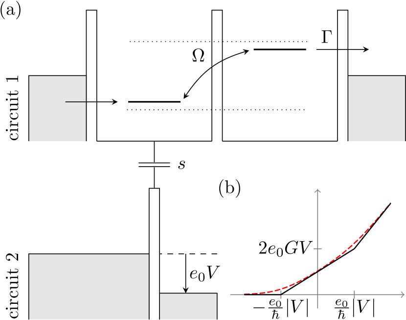
Figure 1: (a) Double quantum dot (DQD, circuit 1) coupled to a quantum point contact (QPC, circuit 2) operated in the weak tunneling regime. The QPC bias voltage $V$ shifts the chemical potential of the right lead by $\mu=-e_{0}V$. (b) Correlation function $C(\omega)=C_{+}(\omega)+C_{-}(\omega)$ of the operator $\Lambda$ by which the QPC couples to the left quantum dot for zero temperature (solid line) and $k_{B}T=0.24eV$ (dashed), see Eqs. (4) and (8).

By now most quantum dots are designed with a nearby quantum point contact (QPC) whose conductance is affected by the charge state of the dot [1, 2]. Then the QPC can act as monitor for the dot charge and provide time-resolved information from which the counting statistics of the electrons flowing through the quantum dot [3, 4] and current correlation functions [5] can be reconstructed. When several quantum dots are strongly tunnel coupled, the wavefunction of their electrons becomes delocalized. Then charge detection corresponds to the measurement of the electron position and causes decoherence and localization. A quantitative analysis [6] revealed that for a double quantum dot (DQD), good measurement correlations can be obtained only at the expense of a backaction strong enough to turn coherent inter-dot tunneling into classical hopping.

Charge transport in a QPC in the weak tunnel limit consists of uncorrelated events in which an electron jumps from one lead to the other [7]. In technical terms, it represents a Poisson process whose fluctuations are non-thermal and known as shot noise [8]. When acting upon a quantum system, these fluctuations not only cause decoherence, but also excite electrons and drive the system out of equilibrium. In this way, the QPC may play a constructive role. In a asymmetric DQD (upper circuit in Fig. 1), shot noise may induce a ratchet current [9].

Coupled conductors can also be used for testing exchange fluctuation relations [10, 11, 12, 13] which are generalized equilibrium relations based on the assumption that each lead is in a Gibbs state. Then forward and backward rates are related by a Boltzmann factor which provides relations between transport coefficients. A prominent example is the Johnson-Nyquist relation between the conductance and the zero-frequency limit of the current correlation function [10, 11]. While exchange fluctuation relations are exact, practical computations of transport properties often rely on approximations such as perturbation theory in the dot-lead tunneling, which may violate exact formal relations. In turn, exact fluctuation relations can be used to test the consistency of theoretical methods. In this spirit, it has been shown [14] that the Bloch-Redfield master equation [15]—despite being a successful, widely applied, and fairly reliable approach—is not always fully compatible with exchange fluctuation relations.

In this work, we address two aspects of transport in capacitively coupled conductors: First, we compute a set of transport coefficients which can be used to experimentally test fluctuations relations along the lines of Refs. [16, 17]. Moreover, we investigate to which extent our master equation results agree with exact formal relations. Second, we characterize the non-equilibrium current through a DQD induced by the coupling to a QPC and study cross correlations between these subsystems.

2 Model and master equation approach

2.1 DQD coupled to a QPC in the tunnel limit

The model sketched in Fig. 1 consists of two electric circuits, the upper one being a DQD coupled to electron source and drain. We describe the DQD by two levels tunnel coupled with matrix element $\Omega$ and detuned by $\epsilon$ such that the one-electron states are split by $\Delta=\sqrt{\epsilon^{2}+\Omega^{2}}$. Thus,

$$H_{\text{DQD}}=\frac{\epsilon}{2}(c_{2}^{\dagger}c_{2}-c_{1}^{\dagger}c_{1})+\frac{\Omega}{2}(c_{1}^{\dagger}c_{2}+c_{2}^{\dagger}c_{1})+Un_{1}n_{2},$$ (1)

where the fermionic operators $c_{1}$ and $c_{2}$ annihilate an electron on the respective dot. The last term of $H_{\text{DQD}}$ accounts for inter-dot Coulomb interaction with strength $U$, while we assume that the repulsion within one dot inhibits double occupation. We will not study spin effects and, thus, work with spinless electrons. The leads are described by $H_{\text{leads}}=\sum_{q}\epsilon_{q}(n_{L,q}+n_{R,q})$ with $n_{\alpha,q}=c_{\alpha,q}^{\dagger}c_{\alpha,q}$ the occupation number of mode $q$ in lead $\alpha=L,R$. The coupling between the leads and the dots is given by

$$H_{\text{DQD-leads}}=\sum_{q}V_{L,q}c^{\dagger}_{L,q}c_{1}+\sum_{q}V_{R,q}c^{\dagger}_{R,q}c_{2}+\text{h.c.},$$ (2)

where “h.c.” denotes the Hermitean conjugate. The effective coupling is given by the spectral density $\Gamma=2\pi\sum_{q}|V_{L/R,q}|^{2}\delta(\epsilon-\epsilon_{q})$ which we assume energy independent. It provides the dot-lead rate $\Gamma/\hbar$.

Our second system is a QPC between two leads modelled by the Hamiltonian $H_{\text{QPC}}=\sum_{k}\epsilon_{k}c_{k}^{\dagger}c_{k}+\sum_{k^{\prime}}\epsilon_{k^{\prime}}c_{k^{\prime}}^{\dagger}c_{k^{\prime}}$, where $k$ and $k^{\prime}$ label the modes of the left and the right lead, respectively. The leads are weakly coupled by the tunnel Hamiltonian $\Lambda=\Lambda_{+}+\Lambda_{-}$, where

$$\Lambda_{+}=\sum_{k,k^{\prime}}t_{kk^{\prime}}c_{k^{\prime}}^{\dagger}c_{k},$$ (3)

transfers an electron from the left to the right QPC lead, while $\Lambda_{-}=\Lambda_{+}^{\dagger}$ describes the opposite process. In a continuum limit, the matrix elements $t_{kk^{\prime}}$ are encompassed by the energy-independent QPC conductance $G=2\pi\sum_{kk^{\prime}}|t_{kk^{\prime}}|^{2}\delta(\epsilon-\epsilon_{k})\delta(\epsilon-\epsilon_{k^{\prime}})$ in units of the conductance quantum $G_{0}=e_{0}^{2}/h$. If an electron resides on dot 1, Coulomb repulsion enhances the barrier between the leads and, thus, reduces the tunnel matrix elements $t_{kk^{\prime}}$. This effect is captured by a prefactor $x=(1-sn_{1})$ in the tunnel Hamiltonian such that

$$H_{\text{QPC}}^{\text{tun}}=x(\Lambda_{+}+\Lambda_{-})=(1-sn_{1})(\Lambda_{+}+\Lambda_{-})$$ (4)

accounts for both the QPC and its coupling to the DQD. For consistency, the dimensionless coupling $s$ must obey $s\leq 1$.

2.2 Master equation and full-counting statistics

Our theoretical description is based on the formal elimination of all four leads such that we remain with a reduced master for the DQD. After transforming the Liouville-von Neumann equation for the total density operator into the interaction picture with respect to $H_{\text{DQD}}$ and the lead Hamiltonians, we derive a Markovian master equation [18] that captures the remaining terms to second order,

$$\dot{\rho}=-\frac{i}{\hbar}[H_{S},\rho]-\frac{1}{\hbar^{2}}\sum_{n}\int\limits_{0}^{\infty}dt\,\operatorname{tr}_{\textrm{leads}}[V_{n},[\tilde{V}_{n}(-t),\rho\otimes R_{0}]],$$ (5)

where $\rho$ is the reduced DQD density operator. $R_{0}$ refers to the grand canonical ensemble of each lead $\alpha$ with a chemical potential shift $\mu_{\alpha}$ measured with respect to a common Fermi energy $\epsilon_{F}$. The operators $V_{n}$ represent $H_{\text{QPC}}^{\text{tun}}$ and the two tunnel contributions of $H_{\text{DQD-leads}}$.

While the reduced master equation (5) fully describes the DQD, the lead degrees of freedom are traced out, so that information about the transported electrons gets lost. To be able to recover it, we multiply before tracing out the leads the full density operator $\rho\otimes R_{0}$ by a phase factor $e^{i\bm{\chi}\cdot\bm{N}}$, where the elements of the vectors $\bm{\chi}=(\chi_{L},\chi_{R},\chi_{\text{QPC}})$ and $\bm{N}=(N_{L},N_{R},N_{\text{QPC}})$ refer to the left and the right lead of the DQD and to the QPC, respectively. Then we obtain the master equation $\dot{\rho}=\mathcal{L}({\bm{\chi}})\rho$ with the generalized Liouvillian $\mathcal{L}({\bm{\chi}})\rho=-(i/\hbar)[H_{\text{DQD}},\rho]+\mathcal{L}_{\text{DQD-leads}}({\bm{\chi}})\rho+\mathcal{L}_{\text{QPC}}({\bm{\chi}})\rho$. The now $\bm{\chi}$-dependent $\rho$ obeys $\operatorname{tr}\rho=\langle e^{i\bm{\chi}\cdot\bm{N}}\rangle$, i.e., it is a generating function from which the moments of the lead electron distributions can be computed by taking derivatives with respect to components of $\bm{\chi}$. Accordingly, $Z(\bm{\chi})\equiv\frac{\partial}{\partial t}\ln\operatorname{tr}\rho$ generates current cumulants, while derivatives at different times provide current correlation functions. After multiplication with the appropriate power of the electron charge $-e_{0}$, we obtain the currents as the corresponding change of the lead electron number: $I_{2}=-ie_{0}\partial Z/\partial\chi_{\text{QPC}}$ and $I_{1}=(-ie_{0}/2)(\partial Z/\partial\chi_{L}-\partial Z/\partial\chi_{R})$ evaluated at $\bm{\chi}=\bm{0}$. The definition of $I_{1}$ is motivated by displacement currents in the leads which have the consequence that primarily the symmetrized current is experimentally accessible. While being irrelevant for the average current, this affects time-dependent quantities such as correlation functions [8].

The evaluation of $\mathcal{L}_{\text{DQD-leads}}({\bm{\chi}})$ for the incoherent DQD-lead tunneling is rather standard, see e.g. the appendix of Ref. [19]. It essentially consists of jump operators between many-particle DQD states that differ by one electron. The transition rates contain Fermi functions reflecting the initial occupation of the lead modes. The elimination of $H_{\text{QPC}}^{\text{tun}}$, by contrast, is way less common and, moreover, describes the interaction of the two circuits which is in the focus of the present article. Therefore it is worthwhile to discuss it in more detail.

By evaluating the $t$-integral in Eq. (5) we end up with the QPC part master equation given by

$$\mathcal{L}_{\text{QPC}}(\bm{\chi})=\mathcal{L}_{\text{QPC}}+(e^{i\chi_{\text{QPC}}}-1)\mathcal{J}^{+}+(e^{-i\chi_{\text{QPC}}}-1)\mathcal{J}^{-}.$$ (6)

Its first term is the QPC Liouvillian

$$\begin{split}\mathcal{L}_{\text{QPC}}\rho=\frac{1}{2\hbar^{2}}\int_{-\infty}^{+\infty}dt\;C(t)\big{[}&\tilde{x}(-t)\rho x+x\rho\tilde{x}(t)\\ -&x\tilde{x}(-t)\rho-\rho\tilde{x}(t)x\big{]}.\end{split}$$ (7)

The symmetrization of the time integral corresponds to neglecting energy renormalization stemming from principal values. A main ingredient to $\mathcal{L}_{\text{QPC}}$ is the correlation function of the QPC tunnel operator, $C(t)=\langle\Lambda(t)\Lambda(0)\rangle=C_{+}(t)+C_{-}(t)$, where $C_{\pm}(t)=\langle\Lambda_{\mp}(t)\Lambda_{\pm}(0)\rangle$ is readily evaluated from its definition and the assumption that the leads are voltage biased. In Fourier representation it reads [7]

$$C_{\pm}(\omega)={} G\,\frac{\hbar\omega\pm e_{0}V}{1-\exp[-(\hbar\omega\pm e_{0}V)/k_{B}T]}$$ (8)

$$={} C_{\mp}(-\omega)e^{(\hbar\omega\pm e_{0}V)/k_{B}T},$$ (9)

see sketch in Fig. 1(b). For energy absorption from the environment, it is evaluated at negative frequencies, for emission at positive frequencies. In the low-temperature limit, $C(\omega)$ vanishes for $\hbar\omega<-|e_{0}V|$, which means that the size of the energy quanta absorbed by the DQD is limited by the QPC bias. Interestingly enough, $C_{\pm}$ can be written in terms of $\epsilon[1-\exp(\epsilon/k_{B}T)]^{-1}$, an expression appearing in master equations for Ohmic quantum dissipation.

The second and third term in Eq. (6) stem from the counting field and vanish for $\chi_{\text{QPC}}\to 0$. The superoperator

$$\mathcal{J}_{+}\rho=\frac{1}{2\hbar^{2}}\int_{-\infty}^{+\infty}dt\;C_{+}(t)\big{[}\tilde{x}(-t)\rho x+x\rho\tilde{x}(t)\big{]}$$ (10)

describes forward tunneling, while backward tunneling is given by the corresponding expression with $C_{-}(t)$.

For the numerical treatment, we decompose the superoperators into the eigenstates of $H_{\text{DQD}}$. In this basis, the interaction picture operators contain time-dependent phase factors, so that the time integrals yield delta functions and, finally, $C_{\pm}(\omega)$ has to be evaluated at the transition frequencies of the DQD. Thus, we have obtained an explicit representation of the Liouvillian $\mathcal{L}(\bm{\chi})$ which provides access to correlation functions [6], current cumulants [20], and transport coefficients [14]. Details for each method can be found in the respective quoted reference.

3 Exchange fluctuation relations

For typical system-lead models, one can write a formally exact expression for the cumulant generating function $Z$ beyond the present perturbation theory. While generally such expressions cannot be evaluated exactly, they provide formal properties such as the so-called exchange fluctuation relation [11]

$$Z(\bm{\chi})=Z(-\bm{\chi}-i\bm{\mu}/k_{B}T),$$ (11)

where $Z(\bm{\chi})$ implicitly depends on the chemical potentials $\bm{\mu}$. The derivation of this relation is based on the assumption that each lead consists of a continuum of modes initially in a Gibbs state, while the central system (here: the DQD) possesses only a few degrees of freedom. A main interest in such relations stems from the fact that the Taylor coefficients of $Z$ at $\bm{\mu}=\bm{\chi}=\bm{0}$ are transport coefficients, i.e., experimentally accessible quantities such as the conductivity. Hence, Eq. (11) provides relations between transport coefficients known as Onsager-Casimir relations [11].

To highlight the relation between the cumulant generating function $Z$ and Casimir-Onsager relations, we notice that by construction, the electron number in lead $\alpha$ changes by the current $I_{\alpha}=-ie_{0}\partial Z/\partial\chi_{\alpha}|_{\bm{\chi}=\bm{0}}$. Moreover, close to equilibrium $\bm{\mu}=\bm{0}$, the current is linear in the voltages. Its slope is a transport coefficient, namely the (trans) conductance $G_{\alpha\beta}=-\partial I_{\alpha}/\partial\mu_{\beta}|_{\bm{\mu}=\bm{0}}$ which obviously is a second derivative of $Z(\bm{\chi})$. Taking the same derivative also on the r.h.s. of Eq. (11) yields $S_{\alpha\beta}/k_{B}T-G_{\alpha\beta}$, where $S_{\alpha\beta}$ is the (co) variance of the currents. Thus, we obtain the Johnson-Nyquist relation $2k_{B}T\,G_{\alpha\beta}=S_{\alpha\beta}$. Generalizing this concept, we define the transport coefficients

$$K^{\alpha_{1}\cdots\alpha_{m}}_{\beta_{1}\cdots\beta_{n}}=\frac{(-i)^{m}\,e_{0}^{m+n}\,\partial^{m+n}}{\partial\chi_{\alpha_{1}}\cdots\partial\chi_{\alpha_{m}}\partial\mu_{\beta_{1}}\cdots\partial\mu_{\beta_{n}}}Z_{(}\bm{\chi})\Big{|}_{\bm{\chi}=\bm{\mu}=\bm{0}}\,.$$ (12)

Applying the same derivative to Eq. (11) provides generalized Casimir-Onsager relations, which we abbreviate as $R^{\alpha_{1}\cdots\alpha_{m}}_{\beta_{1}\cdots\beta_{n}}=0$. For example, $R_{\beta}^{\alpha}=0$ denotes the Johnson-Nyquist relation.

Since approximation schemes are not necessarily consistent with exact formal properties, the question arises whether our master equation approach complies with Eq. (11). Its consistency has been verified for various specific situations [21, 22, 23, 24, 25, 26], while a general proof has been given only in the classical limit [12, 13] and within rotating-wave approximation (RWA) in the single-particle limit [12] and for many-particle states [14]. Beyond RWA, Eq. (11) may be compromised. The deviations, however, tend to be tiny, in particular in the low-temperature limit [14] which is non-trivial since the temperature appears in the denominator. Here we explore the situation for a master equation with the non-conventional Liouvillian $\mathcal{L}_{\text{QPC}}$. In doing so, we extend the results of Refs. [17, 23] to the presence of quantum coherence and those of Ref. [14] to the coupling to a QPC.

3.1 Bloch-Redfield equation in RWA

In the limit of very weak coupling between the central system and the leads, the reduced density operator becomes eventually diagonal in the energy basis defined by $H_{\text{DQD}}|\alpha\rangle=E_{\alpha}|\alpha\rangle$. Thus, one often can work with the ansatz $\rho_{\alpha\beta}=P_{\alpha}\delta_{\alpha\beta}$ which provides the Pauli-type master equation $\dot{P}_{\alpha}=\sum_{\alpha^{\prime}}W_{\alpha\alpha^{\prime}}(\bm{\chi})P_{\alpha^{\prime}}$. The transitions rates $W_{\alpha\alpha^{\prime}}(\bm{\chi})$ follow from a basis decomposition of the master equation (5) after having introduced the counting variables $\bm{\chi}=(\chi_{L},\chi_{R},\chi_{\text{QPC}})$. For our later reasoning, it is important that the long-time solution of a Markovian master equation is dominated by the eigenvalue $-\lambda_{0}(\bm{\chi})$ of the corresponding matrix $W(\bm{\chi})$ that vanishes in the limit $\bm{\chi}\to\bm{0}$, i.e., the one that corresponds to the stationary solution in the absence of the counting variable. Then $P\sim e^{-\lambda_{0}(\bm{\chi})t}$ which translates to $Z=-\lambda_{0}$ and implies that the generating function can be traced back to the computation of an eigenvalue of $W(\bm{\chi})$ [27]. Hence we can conclude that our RWA master equation complies with Eq. (11) if $W(\bm{\chi})$ and $W(-\bm{\chi}-i\bm{\mu}/k_{B}T)$ are isospectral. For the Liouvillian of the type $\mathcal{L}_{\text{DQD-leads}}$ for the dot-lead tunneling, this has already been demonstrated in Ref. [14]. Thus, we can restrict ourselves to the corresponding calculation for $\mathcal{L}_{\text{QPC}}(\bm{\chi})$ in Eq. (6).

By evaluating $W_{\alpha\alpha^{\prime}}(\bm{\chi})$ for $\mathcal{L}_{\text{QPC}}$ and $\mathcal{J}_{\pm}$, see Eqs. (7) and (10), we find

$$W_{\alpha\alpha^{\prime}}(\bm{\chi})=e^{i\chi_{\text{QPC}}}w_{\alpha\leftarrow\alpha^{\prime}}^{+}+e^{-i\chi_{\text{QPC}}}w_{\alpha\leftarrow\alpha^{\prime}}^{-},\quad\alpha\neq\alpha^{\prime}$$ (13)

with the QPC forward and backward rates

$$w_{\alpha\leftarrow\alpha^{\prime}}^{\pm}=C_{\pm}(E_{\alpha^{\prime}}-E_{\alpha})|\langle\alpha|x|\alpha^{\prime}\rangle|^{2}.$$ (14)

Since the Liouvillian $\mathcal{L}(\bm{0})$ conserves the trace of the density matrix, we can obtain the diagonal elements $W_{\alpha\alpha}$ from the normalization condition $\sum_{\alpha}\dot{P}_{\alpha}=0$ yielding $W_{\alpha\alpha}=-\sum_{\alpha^{\prime}\neq\alpha}W_{\alpha^{\prime}\alpha}(\bm{0})$. Using Eq. (9) for $\mu=-e_{0}V$, we find for the QPC contribution by straightforward algebra the relation

$$W_{\alpha\alpha^{\prime}}(-\chi_{\text{QPC}}-i\mu/k_{B}T)=e^{E_{\alpha^{\prime}}/k_{B}T}W_{\alpha^{\prime}\alpha}(\chi_{\text{QPC}})e^{-E_{\alpha}/k_{B}T}.$$ (15)

Together with the corresponding relation for the dot-lead tunneling [14], we obtain

$$W(\bm{\chi})^{T}=S^{-1}W(-\bm{\chi}-i\bm{\mu}/k_{B}T)S,\quad S=e^{-H_{\text{DQD}}/k_{B}T},$$ (16)

where $T$ denotes matrix transposition. This means that the RWA Liouvillian with the modified counting variable relates to the original one by a transposition and a similarity transformation which both leave the eigenvalues invariant. Therefore, we can conclude that the RWA master equation agrees with the exchange fluctuation relation (11).

3.2 Deviations and experimental tests

Despite possessing the desirable consistency with Eq. (11), a RWA master equation has obvious limitations when off-diagonal density matrix elements play a role. This is, e.g., the case for a strongly biased, but undetuned DQD in which the inter-dot tunneling is weaker than the dot-lead tunneling. Then an electron that enters from the source will stay on dot 1 for a while until it proceeds to dot 2. From there it will tunnel rapidly to the drain. Thus, the DQD will will predominantly be in the state $c_{1}^{\dagger}|0\rangle$, so that its density operator in the energy basis has a large off-diagonal contribution and the RWA will fail [28]. As a drawback, however, a treatment beyond RWA is generally not fully consistent with exchange fluctuation relations [14], which motivates a quantitative study of possible discrepancies.

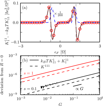
Figure 2: (a) Transport coefficients $K_{1}^{11}$ (solid line) and $-K_{11}^{1}$ (circles) computed with our Bloch-Redfield master equation as a function of the Fermi energy for coupling $s=1$, QPC conductance $G=1$, temperature $T=0.1\Omega/k_{B}$, and the DQD parameters $\Gamma=\epsilon=2U=\Omega$. While according to the exchange fluctuation relation must be differ only by a factor $k_{B}T$, the master equation predicts an additional tiny spurious deviation (dashed line). The vertical lines mark the location of the conductance peaks as discussed in the text. (b) Scaling of the deviations for $k_{B}TK_{11}^{1}+K_{1}^{11}$ and $K^{111}$ from their exact theoretical value zero as a function of the QPC conductance for $\epsilon_{F}=U+\Delta/2$.

Experimentally, the cumulant generating function is not directly accessible and, thus, one may test instead Casimir-Onsager relations derived from it. We here focus on transport coefficients that have been tested with an Aharonov-Bohm ring [16] and a DQD coupled to a QPC [17]. We start with the Johnson-Nyquist relation and find in accordance with Ref. [14] that it is fulfilled within our numerical precision.

Thus, for revealing possible discrepancies, we have to employ Casimir-Onsager relations of higher order such as $k_{B}TK_{11}^{1}+K_{1}^{11}=0$ which follows directly from $R_{11}^{1}=0$ and $R^{111}=0$. Figure 2(a) depicts the master equation result for both terms involved in this relation. Their main contribution appears at the conductance peaks, i.e., at Fermi energies that obey $E^{(n+1)}=E^{(n)}+\epsilon_{F}$, where $E^{(n)}$ is the energy of the lowest state with $n$ electrons on the DQD. Here, $E^{(0)}=0$, $E^{(1)}=-\frac{1}{2}\sqrt{\epsilon^{2}+\Omega^{2}}$, and $E^{(2)}=U$, as can be readily verified by diagonalizing $H_{\text{DQD}}$ in Fock basis. The interpretation of this condition is that an electron from the Fermi surface can tunnel between the lead and the DQD without energy cost, so that already a small voltage can induce a current. With the scale chosen, $k_{B}TK_{11}^{1}$ and $K_{1}^{11}$ appear identical as they ideally should be. A closer look, however, reveals a relative difference of the order $10^{-3}$. Such tiny differences are beyond the resolution of related experiments [16, 17], which lets us conclude that our master equation treatment is sufficiently precise to compute the quantities employed for typical tests of exchange fluctuation relations.

Beyond such practical issues, it is interesting to see how these discrepancies scale with the system parameters. For the “conventional” dot-lead jump operators such as those in $\mathcal{L}_{\text{DQD-leads}}$, one generically finds for small dot-lead rate $R\propto\Gamma^{3}$, while for small inter-dot tunneling, $R\propto\Omega^{2}$ [14]. For $\mathcal{L}_{\text{QPC}}$, see Eq. (6), the relevant parameters are the dimensionless coupling $s$ and the QPC conductance $G$, which brings the scaling as a function of $s$ and $G$ to our attention. Figure 2(b) depicts the peak values of the deviation shown in Fig. 2(a). It indicates that $k_{B}TK_{11}^{1}+K_{1}^{11}\propto s^{2}G$. In particular for $s=0.1$, the l.h.s. of this relation involves computing the tiny difference between two much larger numbers, which is at the limit of our numerical precision. Indeed one notices that for small values of $G$, the data is compromised by numerical errors. We therefore also studied the Casimir-Onsager relation $K^{111}=0$ which follows from $R^{111}=0$. Since this relation consists of only one transport coefficient, it does not suffer from the mentioned numerical problem. The corresponding data in Fig. 2(b) confirms for the deviations the scaling $\propto G$ and $\propto s^{2}$.

Thus we can conclude that the full Bloch-Redfield master equation for the QPC coupling is consistent with exchange fluctuation relations up to corrections $R\propto s^{2}G$, i.e, corrections linear in $G$. By contrast, the mentioned scaling with the DQD parameters $\Gamma$ and $\Omega$ is more favorable [14]. Nevertheless, the Bloch-Redfield approach can be safely applied for the computation of transport coefficients up to second order and when a RWA treatment is sufficient.

4 Tunnel contact as driving source

When non-equilibrium noise acts upon the DQD, it will induce electron transitions from the ground state of the DQD to the excited state, see Fig. 1(a). Once in the excited state, the electron will leave predominantly to the right lead, while subsequently an electron from the left lead enters. In this way, the QPC can spurs a directed current in an unbiased DQD circuit. Its direction depends on the sign of $\epsilon$, which implies a current reversal point at $\epsilon=0$. For strong DQD detuning, this mechanism has been proposed as noise detector [29]. Going beyond that work, our master equation description starts from a complete model that includes the noise source. Moreover, it allows us to study also the backaction on the QPC as well as cross correlations between the circuits.

4.1 Ratchet current

To estimate the ratchet current, we compute the rates for the scenario sketched above. A main role is played by electron transitions from the one-electron ground state of the DQD, $|g\rangle=|1\rangle\cos\phi+|2\rangle\sin\phi$ to the excited state $|e\rangle=-|1\rangle\sin\phi+|2\rangle\cos\phi$, where $\cos(2\phi)=\epsilon/\Delta$ and $|n\rangle=c_{n}^{\dagger}|0\rangle$. These transitions are induced by the Hamiltonian (4), and occur with the golden-rule rate $\gamma=(s^{2}/4)\sin^{2}(2\phi)C(-\Delta/\hbar)/\hbar$. The first factor of this expression stems from the matrix element $\langle e|n_{1}|g\rangle$ and accounts for the delocalization of the DQD orbitals.

When the electron has reached the excited state, it can leave the DQD through either lead, with a probability that depends on the overlap of $|e\rangle$ with the localized states $|1\rangle$ and $|2\rangle$. The corresponding probabilities read $|\langle 1|e\rangle|^{2}=\sin^{2}\phi$ and $|\langle 2|e\rangle|^{2}\cos^{2}\phi$. Since these transitions contribute to the current with opposite sign, we finally obtain $I=e_{0}\gamma(\cos^{2}\phi-\sin^{2}\phi)$, which can be written as

$$I=\frac{e_{0}}{\hbar}\frac{s^{2}\epsilon\Omega^{2}}{4(\epsilon^{2}+\Omega^{2})^{3/2}}C(-\Delta/\hbar).$$ (17)

This expression generalizes the result of Ref. [29] to the regime $|\epsilon|\lesssim\Omega$, in which we expect current reversals as a most relevant feature for possible applications.

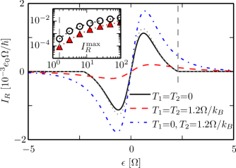
Figure 3: Ratchet current through the DQD as a function of the detuning $\epsilon$ for tunneling matrix element $\Omega=10\Gamma$, QPC conductance $G=1$ and voltage $V=2.5\Omega/e_{0}$, coupling strength $s=0.1$, interaction $U=50\Omega$, and various temperatures. The dotted line marks the analytical solution (17) for $k_{B}T=0$. The vertical lines marks the condition $\epsilon^{2}+\Omega^{2}=(e_{0}V)^{2}$ beyond which the DQD splitting is always larger than $e_{0}V$. Inset: current maximum as a function of the QPC bias voltage $V$ for $k_{B}T=0$ (circles) and $k_{B}T=1.2\Omega$ (triangles) in units of $e_{0}\Omega/\hbar$.

Our numerical solution allows refining the picture drawn by the golden-rule calculation. Figure 3 shows the ratchet current as a function of the DQD detuning, which for zero temperature by and large confirms the behavior predicted by Eq. (17), but indicates that the analytic approach overestimates the ratchet effect. When the QPC temperature is increased, its current acquires a thermal component so that the effective driving becomes stronger. Accordingly, we witness an enhancement of the the ratchet current. By contrast, when both the QPC temperature and the DQD temperature are increased simultaneously, the bias voltage plays a smaller role and both circuits are dominated by thermal noise. Eventually the system reaches thermal equilibrium in which the current vanishes. The dashed line in Fig. 3 shows that already for the moderate temperature $T=1.2\Omega/k_{B}$, the ratchet current is significantly smaller than at $T=0$.

The limitations of our analytic approach are also visible in the current maxima. While Eq. (17) for $e_{0}V\gg\epsilon$ predicts a linear increase with $V$, the data shown in the inset of Fig. 3 demonstrates a sub-linear growth. This deviation is even more clearly visible in the ratchet current as a function of the QPC bias $V$ for constant detuning (inset of Fig. 4). The main reason for this discrepancy is that our analytic approach is based on the assumption that the intra-dot excitation is the slowest process and, thus, governs the dynamics. Upon increasing $V$, however, this assumption will be violated at some stage and we would have to employ rate equation description along the lines of Ref. [30] which considers also the de-excitation $|e\rangle\to|g\rangle$.

4.2 Current noise and cross correlations

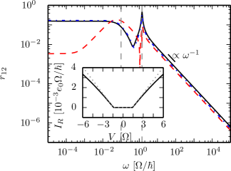
Figure 4: Absolute value of the correlation coefficient $r_{12}$ between the DQD current and the QPC current as a function of the frequency for the detuning $\epsilon=\Omega$. All other parameters are as in Fig. 3. The vertical lines mark the values $\omega=\Gamma/\hbar$ and $\omega=\Delta/\hbar$, respectively. The inset shows the ratchet current in dependence on the applied bias voltage for zero temperature (solid line) and for $k_{B}T=1.2\Omega$ (dotted).

To characterize current fluctuations, we consider the correlation functions $S_{\alpha\beta}(t-t^{\prime})=\langle I_{\alpha}(t)I_{\beta}(t^{\prime})-\langle I_{\alpha}\rangle\langle I_{\beta}\rangle$, where $\alpha$ and $\beta$ label the two circuits. For the auto-correlations we find in the frequency domain roughly $S_{\alpha\alpha}(\omega)\approx\langle I_{\alpha}\rangle$ (not shown), i.e., the typical frequency-independent value for the shot noise of a Poisson process [31]. The physical picture behind this behavior is that of uncorrelated tunnel events which holds for a tunnel contact in the low-temperature regime as well as for the DQD in the regime in which the transitions $|g\rangle\to|e\rangle$ represent the bottleneck for the electron flow.

Let us turn to the cross correlation $S_{12}$ which contains information about the mutual influence of the circuits on each other. A qualitative picture of the physical process emerges from normalized correlations. In the spirit of full-counting statistics of mesoscopic transport, it is common to define the Fano factors $F_{\alpha\alpha}(\omega)=S_{\alpha\alpha}(\omega)/I_{\alpha}$ and the cross Fano factor $F_{12}(\omega)=S_{12}(\omega)/\sqrt{I_{1}I_{2}}$. These quantities relate to the $g^{(2)}$ function in optics and hint on bunching and anti-bunching of transport events [8, 32]. In a typical experimental realization, the currents in the two circuits may differ by several orders of magnitude [9]. Therefore we are not so much interested in correlated counting, but rather in the correlation coefficient $r_{12}(\omega)=S_{12}(\omega)/\sqrt{S_{11}(\omega)S_{22}(\omega)}$ which is normalized to the frequency-dependent auto-correlations. In our case, $r_{12}(\omega)$ and $F_{12}(\omega)$ are practically the same owing to the prevailing Poissonian nature of each current and the corresponding almost constant $S_{\alpha\alpha}(\omega)$.

Figure 4 shows the correlation coefficient for various temperatures. It is characterized by two energies. Below the dot-lead coupling $\Gamma$, we find a plateau after which a decay $\propto\omega^{-1}$ sets in. At the level splitting of the DQD, $\Delta$, we find a peak with a value up to $r_{12}(\Delta/\hbar)\approx 0.85$ indicating strong correlations between the ratchet current and the QPC at resonance. Thus, correlations mainly appear when the QPC can induce resonant transitions between DQD orbitals. The sharp Lorentzian form of the peak indicates the relevance of quantum coherence, which implies that this feature is beyond the treatment with rate-equations that leads to the analytic solution (17). For smaller values of $\Delta$, coherence eventually gets lost and the peak submerges below the low-frequency plateau. As expected for a coherence effect, the peak becomes smaller at higher temperatures.

5 Conclusions

We have investigated a setup composed of two capacitively interacting nano conductors, namely a QPC in the weak tunneling limit and a DQD. While in most recent experimental realization of such setups, the QPC serves as charge monitor for the DQD, we were interested in aspects beyond that. In particular, we focused on the non-equilibrium DQD dynamics induced by the shot noise of the QPC current and on testing the validity of exchange fluctuation relations.

For the theoretical treatment, we have derived a Bloch-Redfield master equation augmented by a counting variable for the electron number in each lead. This allows one to eliminate the leads within second-order perturbation theory without losing information about the transported electrons. For the dot-lead tunneling, one obtains “conventional” jump operators, while the coupling to the QPC yields dissipative terms resembling those stemming from the coupling to a bosonic heat bath. We demonstrated that within RWA, the resulting unconventional jump operators are fully consistent with exchange fluctuation relations. Beyond RWA, we numerically found deviations which decay linearly with the QPC conductance and quadratically with the coupling. In the experimentally relevant regime, these deviations are rather small and do not inhibit computing with a Bloch-Redfield formalism transport coefficients for testing Casimir-Onsager relations. The Johnson-Nyquist relation even turned out to be fulfilled within our numerical precision.

When using the QPC as a driving source, one can induce a ratchet current in the DQD. As a feature most relevant for applications, it possesses a current reversal as a function of the detuning. While generally the ratchet current reflects the spectrum of the effective noise that the QPC entails on the DQD, our numerical results revealed significant deviations from the behavior found with a simple golden-rule treatment. The correlations between the currents in both circuits are most pronounced at frequencies that correspond to the energy splitting of the DQD, which emphasizes the role of quantum coherence. For a typical inter-dot tunnel coupling of $\Omega=25\mu\mathrm{eV}$, the ratchet current is of the order of several $\mathrm{pA}$, a value that can be measured straightforwardly with present techniques. Given that the setup investigated is common in today’s quantum dot design, we are convinced that our results will inspire future experiments.

- [1] T. Ihn, S. Gustavsson, U. Gasser, B. Küng, T. Müller, R. Schleser, M. Sigrist, I. Shorubalko, R. Leturcq, and K. Ensslin Solid State Commun. 149, 1419 (2009).
- [2] D. Taubert, D. Schuh, W. Wegscheider, and S. Ludwig Rev. Sci. Instrum. 82, 123905 (2011).
- [3] S. Gustavsson, R. Leturcq, B. Simovič, R. Schleser, T. Ihn, P. Studerus, K. Ensslin, D. C. Driscoll, and A. C. Gossard Phys. Rev. Lett. 96, 076605 (2006).
- [4] C. Fricke, F. Hohls, W. Wegscheider, and R. J. Haug Phys. Rev. B 76, 155307 (2007).
- [5] N. Ubbelohde, C. Fricke, C. Flindt, F. Hohls, and R. J. Haug Nature Comm. 3, 612 (2012).
- [6] R. Hussein, J. Gómez-García, and S. Kohler Phys. Rev. B 90, 155424 (2014).
- [7] G. L. Ingold and Yu. V. Nazarov, Charge Tunneling Rates in Ultrasmall Junctions, NATO ASI Series B, Vol. 294, (Plenum, New York, 1992), pp. 21–107.
- [8] Ya. M. Blanter and M. Büttiker Phys. Rep. 336, 1 (2000).
- [9] V. S. Khrapai, S. Ludwig, J. P. Kotthaus, H. P. Tranitz, and W. Wegscheider Phys. Rev. Lett. 97, 176803 (2006).
- [10] D. Andrieux and P. Gaspard J. Stat. Mech. 2006, P01011 (2006).
- [11] K. Saito and Y. Utsumi Phys. Rev. B 78, 115429 (2008).
- [12] M. Esposito, U. Harbola, and S. Mukamel Rev. Mod. Phys. 81, 1665 (2009).
- [13] M. Campisi, P. Hänggi, and P. Talkner Rev. Mod. Phys. 83, 771 (2011).
- [14] R. Hussein and S. Kohler Phys. Rev. B 89, 205424 (2014).
- [15] A. G. Redfield IBM J. Res. Develop. 1, 19 (1957).
- [16] S. Nakamura, Y. Yamauchi, M. Hashisaka, K. Chida, K. Kobayashi, T. Ono, R. Leturcq, K. Ensslin, K. Saito, Y. Utsumi, and A. C. Gossard Phys. Rev. Lett. 104, 080602 (2010).
- [17] Y. Utsumi, D. S. Golubev, M. Marthaler, K. Saito, T. Fujisawa, and G. Schön Phys. Rev. B 81, 125331 (2010).
- [18] A. G. Redfield IBM J. Res. Develop. 1, 19 (1957).
- [19] R. Hussein and S. Kohler Phys. Rev. B 86, 115452 (2012).
- [20] C. Flindt, T. Novotný, A. Braggio, M. Sassetti, and A. P. Jauho Phys. Rev. Lett. 100, 150601 (2008).
- [21] R. Sánchez, R. López, D. Sánchez, and M. Büttiker Phys. Rev. Lett. 104, 076801 (2010).
- [22] G. Bulnes Cuetara, M. Esposito, and P. Gaspard Phys. Rev. B 84, 165114 (2011).
- [23] D. S. Golubev, Y. Utsumi, M. Marthaler, and G. Schön Phys. Rev. B 84, 075323 (2011).
- [24] G. Bulnes Cuetara, M. Esposito, G. Schaller, and P. Gaspard Phys. Rev. B 88, 115134 (2013).
- [25] Y. Utsumi, D. S. Golubev, M. Marthaler, K. Saito, T. Fujisawa, and G. Schön Phys. Rev. B 81, 125331 (2010).
- [26] R. López, J. S. Lim, and D. Sánchez Phys. Rev. Lett. 108, 246603 (2012).
- [27] D. A. Bagrets and Yu. V. Nazarov Phys. Rev. B 67, 085316 (2003).
- [28] F. J. Kaiser, M. Strass, S. Kohler, and P. Hänggi Chem. Phys. 322, 193 (2006).
- [29] R. Aguado and L. P. Kouwenhoven Phys. Rev. Lett. 84, 1986 (2000).
- [30] M. Stark and S. Kohler EPL 91, 20007 (2010).
- [31] N. G. van Kampen, Stochastic processes in physics and chemistry (North-Holland, Amsterdam, 1992).
- [32] C. Emary, C. Pöltl, A. Carmele, J. Kabuss, A. Knorr, and T. Brandes Phys. Rev. B 85, 165417 (2012).