$\bm{1/m}$ Corrections for Orbitally Excited Heavy Mesons and the $\bm{1/2}$ – $\bm{3/2}$ Puzzle

Abstract

We re-investigate the effects of the $1/m_{c}$ corrections on the spectrum of the lowest orbitally excited $D$-meson states. We argue that one should expect the $1/m_{c}$ corrections to induce a significant mixing between the two lowest lying $1^{+}$ states. We discuss the implications of this mixing and compute its effect on the semileptonic decays $B\to D^{**}\ell\bar{\nu}$ and the strong $D^{**}$ decays.

I Introduction

The spectroscopy of excited hadrons containing a heavy quark is determined to a large extend by the fact that the spin of the heavy quark decouples from the light degrees of freedom Isgur and Wise (1991). To this end, the rotations of the heavy quark spin become a symmetry that is not present for light hadrons. As a consequence, all heavy hadrons (with a single heavy quark) fall into spin-symmetry doublets, the members of which are related by a rotation of the heavy quark spin.

For the mesonic ground states, the spin symmetry doublets consist of the $0^{-}$ pseudo scalar meson and the $1^{-}$ vector meson, such as $(D,D^{*})$ and $(B,B^{*})$. For the mesons with one additional unit of angular momentum of the light degrees of freedom two further spin symmetry doublets appear. These correspond to a total angular momentum $j=1/2$ and $j=3/2$ of the light degrees of freedom, respectively. Coupling it to the heavy quark spin and taking into account the factor $(-1)^{\ell+1}$ for the parity, we end up with a doublet with the quantum numbers $(0^{+},1^{+})$ for $j=1/2$ and one with $(1^{+},2^{+})$ for $j=3/2$.

The same systematics continues for higher orbital excitations, i.e. for arbitrary $\ell$ Isgur and Wise (1991). The doublets which emerge have the quantum numbers

$$((\ell-1)^{(-1)^{\ell+1}},\ell^{(-1)^{\ell+1}})\quad\text{for}\quad j=\ell-1/2\,,$$

and

$$(\ell^{(-1)^{\ell+1}},(\ell+1)^{(-1)^{\ell+1}})\quad\text{for}\quad j=\ell+1/2\,.$$

The decoupling of the heavy quark also has interesting consequences for the strong decays of excited heavy hadrons, since these are then governed by the light degrees of freedom only. In this way one may predict the partial waves involved in the strong decays and thus one may predict a specific pattern of angular-momentum suppressions in the strong decays Isgur and Wise (1991); Lu et al. (1992).

In the heavy mass limit the members of the doublets are mass-degenerate, and the splittings between the multiplets are mass independent. Nevertheless, these splittings are of the order of $\Lambda_{\rm QCD}$, since they are related to excitations of the light degrees of freedom.

The $1/m_{c}$ corrections couple the heavy quark spin to the light degrees of freedom, leading also to a splitting within the doublets. However, in particular for the $D$ mesons, the splitting between the multiplets and the ($1/m$ induced) splittings within each of the multiplets are numerically of the same order. Thus a significant mixing of the two $\ell^{(-1)^{\ell+1}}$ states belonging to the two different multiplets must be expected.

Previous analyses of the $1/m_{c}$ corrections also noticed the possibility of this mixing Lu et al. (1992); Kilian et al. (1992); Falk and Mehen (1996); Leibovich et al. (1998); Bernlochner et al. (2012). However, some of the analyses assumed that this effect is small, based on the observation that the two $1^{+}$ states should have different widths, since the strong decays of the $1^{+}$ state with $j=3/2$ correspond to $p$-wave transitions. Since the data indicate that the observed widths indeed follow this pattern, the mixing was assumed to be small.

In the present paper we re-consider this effect and try to estimate the size of the corresponding mixing angle, which can be extracted from the data on the basis of a few model assumptions. Based on this, we extract a mixing angle that is larger than what has been discussed before, and consider the implications in particular for semileptonic $B$ decays into orbitally excited $D$ mesons.

II Orbitally Excited States and the Effect of Mixing

The orbitally excited states fall into two spin-symmetry doublets, classified by their angular momentum of the light degrees of freedom $j$. We shall use the notation

$$\begin{split}\left(\begin{matrix}|D(0^{+})\rangle\\ |D(1^{+})\rangle\end{matrix}\right)\quad&\text{with}\quad j=1/2\,,\\ \left(\begin{matrix}|D^{*}(1^{+})\rangle\\ |D^{*}(2^{+})\rangle\end{matrix}\right)\quad&\text{with}\quad j=3/2\,.\end{split}$$ (1)

In the limit $m_{c}\to\infty$ the members within each of the spin symmetry doublet are degenerate:

$$M(D(0^{+}))=M(D(1^{+})) =m_{c}+\bar{\Lambda}_{1/2}\,,$$ (2)

$$M(D^{*}(1^{+}))=M(D^{*}(2^{+})) =m_{c}+\bar{\Lambda}_{3/2}\,,$$

where $\bar{\Lambda}_{j}$ is the binding energy of the mesons in the limit $m_{c}\to\infty$.

Note that the splitting $\bar{\Lambda}_{3/2}-\bar{\Lambda}_{1/2}$ between the two doublets does not scale with the heavy quark mass. However, it is related to the binding of the light quark within the chromoelectric field of the heavy quark and hence it is of the order of $\Lambda_{\rm QCD}$. In fact, for the $D$ mesons, the current data yield a value of about 20 MeV for this splitting.

Power corrections of order $1/m_{c}$ are induced by the kinetic and the chromomagnetic operator, leading to a Hamiltonian density of the form

$${\cal H}_{1/m}=\frac{1}{2m_{c}}\bar{c}(iD_{\perp})^{2}c+\frac{g_{s}}{2m_{c}}\bar{c}(\vec{\sigma}\cdot\vec{B})c\,.$$ (3)

In particular, the second term couples the heavy quark spin to the light degrees of freedom, which breaks the spin symmetry; however, the angular momentum of the light degrees of freedom $j$ is still a good quantum number.

We are going to consider the effects of ${\cal H}_{1/m}$ on the two spin symmetry doublets shown in eq. (1). First of all, the kinetic energy contribution only leads to a shift of the masses, which we shall absorb into the values of the masses

$$M_{j}=m_{c}+\bar{\Lambda}_{j}+\frac{1}{2m_{c}}\mu_{\pi}^{2}(j)\,,$$ (4)

where $\mu_{\pi}^{2}(j)$ is the kinetic-energy parameter for the orbitally excited meson. The second term in eq. (3), however, leads to the effects, which we shall discuss in some detail. It is related to the chromomagnetic field induced by the light degrees of freedom at the location of the heavy quark spin. Clearly not much is known about this from first principles, so one has to make some assumptions here to arrive at quantitative estimates.

The chromomagnetic field at the location of the heavy quark is generated by the angular momenta of the light degrees of freedom, which is the orbital angular momentum $\vec{L}$ and the spin of the light quark $\vec{s}$, the sum of which constitutes the angular momentum of the light degrees of freedom $\vec{J}$. The complete angular momentum $\vec{K}$ is

$$\vec{K}=\vec{J}+\vec{\sigma}=\vec{L}+\vec{s}+\vec{\sigma}\,.$$ (5)

The key assumption we shall make is that the orbital angular momentum and the light quark spin have different gyro-chromomagnetic factors $\alpha^{\prime}$ and $\beta^{\prime}$, such that the chromomagnetic field seen by the heavy quark is not proportional to the total angular momentum $J$ of the light degrees of freedom:

$$\vec{B}\sim\alpha^{\prime}\vec{L}+\beta^{\prime}\vec{s}=\alpha\vec{J}+\beta\vec{s}\,.$$ (6)

To this end, the second term in eq. (3) can be written as

$$H_{1/m}=\int d^{3}\vec{x}\,\frac{g_{s}}{2m_{c}}\bar{c}(\vec{\sigma}\cdot\vec{B})c=P_{1}(\vec{J}\cdot\vec{\sigma})+P_{2}(\vec{s}\cdot\vec{\sigma})\,,$$ (7)

where the operators $P_{1}$ and $P_{2}$ act only on the radial wave functions of the light degrees of freedom.

We note that the $|D^{*}(2^{+})\rangle$ and the $|D(0^{+})\rangle$ states are eigenstates of the Hamiltonian, even once the above $1/m_{c}$ corrections are included

$$H|D^{*}(2^{+})\rangle =\left(M_{3/2}+\frac{3}{4}g+\frac{1}{4}g^{\prime}\right)|D^{*}(2^{+})\rangle\,,$$ (8)

$$H|D(0^{+})\rangle =\left(M_{1/2}-\frac{3}{4}g+\frac{1}{4}g^{\prime}\right)|D(0^{+})\rangle\,,$$ (9)

where the mass values $M_{1/2}$ and $M_{3/2}$ are the masses defined in eq. (4). Furthermore, the constants $g$ and $g^{\prime}$ are obtained from the radial wave functions, i.e. the matrix elements $g\sim\langle P_{1}\rangle$ and $g^{\prime}\sim\langle P_{2}\rangle$; here we assume for simplicity that $g$ and $g^{\prime}$ are identical for the two doublets. The relevant coefficients are obtained from the spin wave functions discussed in the appendix.

For the two $1^{+}$ states, the second term of eq. (7) induces a mixing, since we have

$$\begin{aligned} H|D(1^{+})\rangle&=\left(M_{1/2}+\frac{1}{4}g-\frac{1}{12}g^{\prime}\right)|D(1^{+})\rangle\\ &\quad+\frac{\sqrt{2}}{3}g^{\prime}\,|D^{*}(1^{+})\rangle\,,\end{aligned}$$ (10)

$$\begin{aligned} H|D^{*}(1^{+})\rangle&=\left(M_{3/2}-\frac{5}{4}g-\frac{5}{12}g^{\prime}\right)|D^{*}(1^{+})\rangle\\ &\quad+\frac{\sqrt{2}}{3}g^{\prime}\,|D(1^{+})\rangle\,,\end{aligned}$$ (11)

where we have – once more – assumed that the relevant matrix elements of $P_{1}$ and $P_{2}$ are identified with the parameters $g$ and $g^{\prime}$. Again, the relevant coefficients in front of $g$ and $g^{\prime}$ follow from the spin wave functions given in the appendix.

Clearly this analysis is drastically simplified, but an improvement would need the reference to some model for the binding dynamics of the orbitally excited mesons. Nevertheless, from this simplified analysis we can infer some information on the mixing angle from the data. First of all – looking at the data summarized in table 1 and schematically shown in figure 1 – we note that the broader $1^{+}$ state has a larger mass than the narrower $1^{+}$ state. From heavy-quark symmetries we infer that the broader states decay through an $S$ wave transition which is possible only for the $j=1/2$ states. The $j=3/2$ states can decay (strongly) only through a $D$ wave transition which is suppressed by angular momentum, rendering these states narrow Isgur and Wise (1991). For this reason we make the assignments shown in table 1.

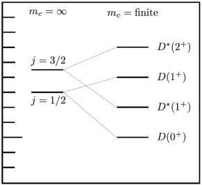
Figure 1: Schematic of the mass hierarchy for the orbitally excited $D$ mesons.

State	Mass [MeV]	Width [MeV]	$j$
$D(0^{+})$	$2318\pm 29$	$267\pm 40$	$1/2$
$D(1^{+})$	$2427\pm 40$	$384\pm 120$	$1/2$
$D^{*}(1^{+})$	$2421.4\pm 0.6$	$27.4\pm 2.5$	$3/2$
$D^{*}(2^{+})$	$2462.6\pm 0.6$	$49\pm 1.3$	$3/2$

Table 1: Averages of the existing mass and width measurements for the $D^{**}$ states according to the PDG Olive et al. (2014). Our choice of the $j$ assignment follows from total decay widths.

Starting from the heavy quark limit, the splitting within the two doublets is induced by $1/m_{c}$ effects. Ignoring their mixing for the moment, the two $1^{+}$ states will cross when we switch on the $1/m_{c}$ terms, leading to the “level inversion” observed in the spectrum depicted in figure 1. Switching on the mixing leads to the well known “level repulsion”, which is shown in figure 2 for the parameter values obtained from the fit discussed below. For the $1^{+}$ states this implies a mixing, which is maximal at the crossing point $|\theta|=45^{\circ}$. In order to explain the assumed “level inversion”, we must have $45^{\circ}\leq|\theta|\leq 90^{\circ}$; i.e., mixing beyond the crossing point.

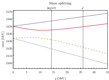
Figure 2: The orbitally excited states in the $j=1/2$ and the $j=3/2$ doublets are degenerate in the infinite mass limit $m_{c}=\infty$, corresponding to $g=g^{\prime}=0$. For a finite mass $m_{c}$ we find a splitting of the states. We plot the masses of the orbitally excited states $D(0^{+})$ (light-blue, long-dashed), $D(1^{+})$ (green, short-dashed), $D^{*}(1^{+})$ (red, solid) and $D^{*}(2^{+})$ (dark blue, dotted) as a function of the parameter $g$. The parameter $g^{\prime}$ is fixed by the condition $g^{\prime}=-g$. The vertical lines indicate the best fit value $g^{*}$ for $g$ and the zero of $\Delta(g,g^{\prime}=-g)$.

For a quantitative analysis, we use our simple assumptions and encode the mixing of the two $1^{+}$ states in the $2\times 2$ sub matrix of the Hamiltonian

$${\bf H}=\left[\begin{array}[]{cc}M&a\\ a&M^{*}\end{array}\right]\,,$$ (12)

and we define

$$M \equiv M_{1/2}+\frac{1}{4}g-\frac{1}{12}g^{\prime}\,,$$ (13)

$$M^{*} \equiv M_{3/2}-\frac{5}{4}g-\frac{5}{12}g^{\prime}\,,$$ (14)

$$\Delta \equiv M^{*}-M=M_{3/2}-M_{1/2}-\frac{3}{2}g-\frac{1}{3}g^{\prime}\,,$$ (15)

$$a \equiv\frac{\sqrt{2}}{3}g^{\prime}\,.$$ (16)

For vanishing $g^{\prime}$ the Hamiltonian becomes diagonal, but in this case the splitting in the $D^{*}(J^{+})$ doublet is twice as large as the one in the $D(J^{+})$. We note that the splittings within each of the doublets is equal if $g=-g^{\prime}$, which we consider as a benchmark point. This point is interesting to consider in terms of our simple model: Assuming that all overlap integrals are equal, we obtain from eq. (6)

$$\vec{B}\sim g\vec{J}+g^{\prime}\vec{s}=g(\vec{J}-\vec{s})=g\vec{L}\,,$$ (17)

which would mean that the spectrum is roughly driven by the orbital angular momentum $L$ of the light degrees of freedom. As a result, the spectrum is independent of the orientation of the light quark spin. However, this could as well be an artifact of our simple assumptions.

To this end, the eigenstates of ${\bf H}$ (i.e., the physical $1^{+}$ states) are thus linear combinations of the states defined in the heavy-mass limit

$$|D_{L}(1^{+})\rangle =\quad\!\cos\theta\,|D(1^{+})\rangle+\sin\theta\,|D^{*}(1^{+})\rangle\,,$$ (18)

$$|D_{H}(1^{+})\rangle =-\sin\theta\,|D(1^{+})\rangle+\cos\theta\,|D^{*}(1^{+})\rangle\,,$$ (19)

where $D_{L}$ ($D_{H}$) is the state with the lower (higher) eigenvalue. The mixing angle $\theta$ satisfies

$$\tan 2\theta=\frac{-2a}{\Delta}=\frac{-4\sqrt{2}g^{\prime}}{6(M_{3/2}-M_{1/2})-9g+2g^{\prime}}\,,$$ (20)

and the corresponding eigenvalues are given by

$$M_{H/L}=\frac{1}{2}\left[(M+M^{*})\pm\sqrt{\Delta^{2}+4a^{2}}\right]\,.$$ (21)

Note that we have always $M_{H}>M_{L}$, reflecting the “level repulsion” of the $2\times 2$ system. The situation of minimal splitting $M_{H}-M_{L}$ corresponds to $\Delta=0$, which yields $|\theta|=45^{\circ}$. This means that the contribution of the $j=3/2$ state in the eigenvector $|D_{L}(1^{+})\rangle$ starts to become dominant, in accordance to the observed level sequence. This is shown in figure 3, where the mixing angle $\theta$ is plotted as a function of $g^{\prime}$, with the constraints $g=-g^{\prime}$. There, the vertical line corresponds to the best-fit value of $g^{\prime}$ of the fit discussed below, where we find a mixing angle of about $60^{\circ}$.

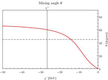
Figure 3: The mixing angle $\theta$ as a function of $g^{\prime}$ and with $g=-g^{\prime}$. The vertical line indicates the best fit point. The horizontal line indicates the maximum-mixing angle of $\theta=45^{\circ}$.

In previous analyses (e.g. in reference Falk and Mehen (1996)), a value for $\theta$ of the order of ten degrees has been considered. However, this is not in contradiction to our discussion, since an interchange of the two $1^{+}$ states corresponds to a replacement $\theta\to 90-\theta$. Nevertheless, we advocate that the magnitude of $\theta$ is larger than considered in previous analyses.

The experimental results for the masses and widths of the orbitally excited $D$ mesons are presently unsettled. The individual results for the masses, for instance, do not agree well with their respective PDG averages Olive et al. (2014). This is evidenced by the application of scale factors to the error on the average values. Nevertheless, we attempt to confront our simple model with the present data.

Mass [MeV]	Pull [$\sigma$]	Reference
$D(0^{+})$
$2297\pm 8$	$-13.75$	Aubert et al. (2009)	$\times$
$2308\pm 36$	$-2.75$	Abe et al. (2004)	$\times$
$2407\pm 41$	$-0.00$	Link et al. (2004)
$D_{L}(1^{+})$
$2423.1\pm 1.8$	$+1.24$	Abramowicz et al. (2013)
$2420.1\pm 0.8$	$-0.95$	del Amo Sanchez et al. (2010)
$2426.0\pm 3.2$	$+1.61$	Abe et al. (2005)
$D_{H}(1^{+})$
$2427\pm 36$	$-0.62$	Abe et al. (2004)
$2477\pm 40$	$+0.69$	Aubert et al. (2006)	$\dagger$
$D^{*}(2^{+})$
$2462.5\pm 2.7$	$+0.01$	Abramowicz et al. (2013)
$2462.2\pm 0.8$	$-0.34$	del Amo Sanchez et al. (2010)
$2464.5\pm 2.2$	$+0.92$	Link et al. (2004)

Table 2: Masses for the various $D^{**}$ measurements. We use up to three of the most precise mass measurements, if available. We also list the pull values at the best-fit point eq. 23. Measurements with a $\times$ mark are not included in the fit, see text. Uncertainties of Measurements with a $\dagger$ mark have been doubled, due to lack of estimates for the systematic uncertainty.

In a first step, we assume $g^{\prime}=-g$, thereby reducing the number of model parameters to three: $M_{1/2}$, $M_{3/2}$, and $g$. This assumption stems from the fact, that the mass splitting of the doublets is equal for $g=-g^{\prime}$, as argued above. We then fit the three parameters to the four PDG averages of the measurements as listed in table 1. Note, that we impose the additional constraint $\Delta<0$, based on the mass hierarchy shown in figure 1. This fit has one degree of freedom (d.o.f.). We reject the fit, since we obtain $\chi^{2}=8.48$ and a p-value of $0.36\%$, which is smaller than our a-priori threshold of $3\%$. While the masses of the two $1^{+}$ eigenstates and the $2^{+}$ state are modelled very well, we find a large pull of slightly less than $3\sigma$ for the $0^{+}$ mass. The best-fit point and the parameter intervals at $68\%$ confidence level (CL) read

$$M^{*}_{1/2} =(2425\pm 2)\text{MeV}\,, M^{*}_{3/2} =(2451\pm 5)\text{MeV}\,,$$ (22)

$$g^{*} =(23\pm 6)\text{MeV}\,.$$

In a second step, we wish to find out which of the individual measurements do not agree well with our model. For this purpose, we use the 11 most precise individual measurements, with up to three measurements per $D^{**}$ state. These measurements also enter the PDG averages, and they are listed in table 2. Given the larger number of measurements, we can now lift the previous assumption and fit all four model parameters. We again impose the theory constraint $\Delta<0$. We reject this fit as well, since for seven d.o.f. we obtain $\chi^{2}=177$, corresponding to a p-value of less than $10^{-10}$. However, we observe that the $\chi^{2}$ is driven by two measurements: the measurements of the $0^{+}$ mass as carried out by the BaBar and Belle collaborations, respectively. It is therefore interesting to repeat this second fit without the BaBar and Belle measurements of $0^{+}$ masses, which we do. We find for this new fit the best-fit point and the $68\%$ CL intervals

$$M^{*}_{1/2} =(2433\pm 4)\text{MeV}\,, M^{*}_{3/2} =(2450\pm 5)\text{MeV}\,,$$ (23)

$$g^{*} =(26\pm 5)\text{MeV}\,, g^{\prime*} =(-27\pm 21)\text{MeV}\,.$$

We also compute the goodness of fit for this reduced data set. We find a good fit for five d.o.f. and $\chi^{2}=6.86$, which corresponds to a p-value of $0.23$. The individual pull values at the best-fit point, defined via

$$\operatorname{pull}_{i}\equiv\frac{M_{i}-M_{i}(M^{*}_{1/2},M^{*}_{3/2},g^{*},g^{\prime*})}{\sigma_{i}}$$ (24)

for every measurement $i$, are listed in table 2. Based on the results of this fit, eq. (23), we find approximately $\Delta\simeq-13$ MeV, as well as $g^{\prime}\simeq-g<0$. This indicates a large mixing, with $\theta=(+59^{+24}_{-14})^{\circ}$ at $68\%$ CL.

Our findings can be summarized as follows: Neither the averages, nor the three most precise measurements of each of the $D^{**}$ masses are fitted well by our simple assumptions. Removing two of the individual measurements of the $0^{+}$ mass from our analysis yields a good fit. In addition, most of the measurements are not in good agreement with each other Olive et al. (2014). On the basis of the current experimental data, the situation remains inconclusive. In our opinion, a simultaneous determination of the masses and widths of all orbitally excited states needs to be undertaken before a definite answer to mixing of the $1^{+}$ states can be given. Within such an analysis, the mixing effects of the decay widths could be taken into account as well.

III Effects on Semileptonic Decays

	$\tau_{1/2}(1)$	$\rho_{1/2}^{2}$	$\tau_{3/2}(1)$	$\rho_{3/2}^{2}$
GI Godfrey and Isgur (1985)	$0.22$	$0.83$	$0.54$	$1.50$
VD Veseli and Dunietz (1996)	$0.13$	$0.57$	$0.43$	$1.39$
CCCN Cea et al. (1988); Colangelo et al. (1991)	$0.06$	$0.73$	$0.51$	$1.45$
ISGW Isgur et al. (1989)	$0.34$	$1.08$	$0.59$	$1.76$

Table 3: Results of the fit of eq. (31) to four different model calculations for the two form factors. (numbers taken from Morenas et al. (1997)).

Exclusive semileptonic $b\to c$ decays are governed by heavy quark symmetry for both the bottom and the charm quark. The decays of $B$ mesons into orbitally excited $D$ mesons have been investigated in the context of heavy quark symmetry in Leibovich et al. (1998), including also the $1/m_{c}$ corrections. As stated above and in contrast to Leibovich et al. (1998), we study a scenario where the mixing is the leading $1/m_{c}$ effect.

In the infinite mass limit, the hadronic weak transition currents can be described by a single Isgur Wise function for each multiplet. Using the spin representations for the states involved

$$\overline{B}(v) =\sqrt{M_{B}}\gamma_{5}\frac{1+\not{v}}{2}\,,$$ (25)

$$D(1^{+};v,\epsilon) =\sqrt{M_{D}}\frac{1+\not{v}}{2}\gamma_{5}\not{\epsilon}\,,$$ (26)

$$D^{*}_{\mu}(1^{+};v,\epsilon) =\sqrt{M_{D^{*}}}\sqrt{\frac{3}{2}}\frac{1+\not{v}}{2}\gamma_{5}$$ (27)

$$\quad\left[\epsilon_{\mu}-\frac{1}{3}\not{\epsilon}(\gamma_{\mu}-v_{\mu})\right]\,,$$

one defines for some current defined by a Dirac matrix $\Gamma$ the two Isgur-Wise functions as Leibovich et al. (1998)

$$\langle B(v)|\bar{b}\Gamma c|D(1^{+};v^{\prime},\epsilon)\rangle\\ =2\,\tau_{1/2}(vv^{\prime}){\rm Tr}\left[\overline{B}(v)\Gamma D(1^{+};v^{\prime},\epsilon)\right]\,,$$ (28)

$$\langle B(v)|\bar{b}\Gamma c|D^{*}(1^{+};v^{\prime},\epsilon)\rangle\\ =\sqrt{3}\,\tau_{3/2}(vv^{\prime})v^{\mu}{\rm Tr}\left[\overline{B}(v)\Gamma D^{*}_{\mu}(1^{+};v^{\prime},\epsilon)\right]\,.$$ (29)

In the above the convention for the two Isgur-Wise functions is the same as in Leibovich et al. (1998) and Biancofiore et al. (2013).

The mixing induced by $1/m_{c}$ effects yields for the hadronic currents

$$\langle B|\bar{b}\Gamma c|D_{L}\rangle =\quad\!\cos\theta\langle B|\bar{b}\Gamma c|D(1^{+})\rangle+\sin\theta\langle B|\bar{b}\Gamma c|D^{*}(1^{+})\rangle\,,$$ (30)

$$\langle B|\bar{b}\Gamma c|D_{H}\rangle =-\sin\theta\langle B|\bar{b}\Gamma c|D(1^{+})\rangle+\cos\theta\langle B|\bar{b}\Gamma c|D^{*}(1^{+})\rangle\,,$$

which can be expressed in terms of the form factors $\tau_{1/2}(\omega)$ and $\tau_{3/2}(\omega)$.

The two form factors are parametrized Morenas et al. (1997) via

$$\tau_{j}(\omega)=\tau_{j}(1)\left[\frac{2}{1+\omega}\right]^{2\rho_{j}^{2}},\qquad j=1/2\text{ or }j=3/2$$ (31)

which is expected to be a reasonable approximation, since the kinematic region turns out to be quite limited: $1\leq\omega\lesssim 1.3$.

Not much is known about the form factors $\tau_{j}(\omega)$. However, there are sum rules constraining these form factors Uraltsev (2001); in particular we have

$$\mu_{\pi}^{2}-\mu_{G}^{2}\leq 9\,\epsilon_{1/2}|\tau_{1/2}(1)|^{2}\,,$$ (32)

where $\mu_{\pi}$ and $\mu_{G}$ are the kinetic energy and chromomagnetic moment parameters, and $\epsilon_{1/2}$ is the excitation energy of the $j=1/2$ doublet above the ground state doublet. Numerically, the left-hand side of this relation is small: $\mu_{\pi}^{2}-\mu_{G}^{2}\ll\mu_{\pi}^{2}$. This motivates the so-called BPS limit, which leads to $\mu_{\pi}^{2}-\mu_{G}^{2}=0$. In this limit we would have $\tau_{1/2}(1)=0$ indicating that the theoretical expectation is that (in the relevant kinematic region)

$$\tau_{1/2}(\omega)\ll\tau_{3/2}(\omega)\,.$$ (33)

In the combined infinite mass and BPS limits this leads to the expectation that the decays into the $D(1^{+})$ are heavily suppressed compared to the ones into the $D^{*}(1^{+})$. Current data do not support this, which constitutes the $1/2-3/2$ puzzle in semileptonic $B$ decays.

Various models and sum rule calculations have been used to obtain more information on the $\tau_{j}(\omega)$. In Table 3 we list some of the currently used models in this context; note that all models reflect the relation eq. (33) in a more or less pronounced way.

Decay mode	$\mathcal{B}$ (%)
${\mathcal{B}}(B^{-}\to D(0^{+})\ell\nu)\times{\mathcal{B}}(D(0^{+})\to D^{+}\pi^{-})$	$0.29\pm 0.05$
${\mathcal{B}}(B^{-}\to D_{L}(1^{+})\ell\nu)\times{\mathcal{B}}(D_{L}(1^{+})\to D^{*+}\pi^{-})$	$0.29\pm 0.14$
${\mathcal{B}}(B^{-}\to D_{H}(1^{+})\ell\nu)\times{\mathcal{B}}(D_{H}(1^{+})\to D^{*+}\pi^{-})$	$0.13\pm 0.04$
${\mathcal{B}}(B^{-}\to D^{*}(2^{+})\ell\nu)\times{\mathcal{B}}(D^{*}(2^{+})\to D^{*+}\pi^{-})$	$0.078\pm 0.008$

Table 4: HFAG averages for the products of the production branching fractions of $B^{-}\to D^{**}\ell\nu$ decays with the decay branching fractions $D^{**}\to D^{(*)+}\pi^{-}$ Amhis et al. (2014). The uncertainties arise from the squared sum of the statistical and systematical uncertainties.

The differential decay rates in the infinite mass limit are well known Leibovich et al. (1998). Including the mixing eq. (30) as the leading $1/m_{c}$ effect one obtains for $B\to D_{L}\ell\bar{\nu}$

$$\frac{d\Gamma}{d\omega} =\frac{G_{F}^{2}V_{cb}^{2}M_{B}^{5}}{24\pi^{3}}\,r_{L}^{3}(\omega-1)\sqrt{\omega^{2}-1}$$ (34)

$$\Big{\{} \quad\sin^{2}\theta(\omega+1)^{2}[2(\omega-r_{L})(1-r_{L}\omega)-(1+r_{L}^{2}-2r_{L}\omega)]|\tau_{3/2}(\omega)|^{2}$$

$$+2\cos^{2}\theta[2r_{L}(\omega^{2}-1)+(5\omega-1)(1+r_{L}^{2}-2r_{L}\omega)]|\tau_{1/2}(\omega)|^{2}$$

$$+2\sqrt{2}\sin\theta\cos\theta(\omega+1)^{2}[(1+r_{L})^{2}-4r_{L}\omega]Re(\tau_{1/2}(\omega)\tau^{*}_{3/2}(\omega))\Big{\}}\,,$$

while we get for $B\to D_{H}\ell\bar{\nu}$

$$\frac{d\Gamma}{d\omega} =\frac{G_{F}^{2}V_{cb}^{2}M_{B}^{5}}{24\pi^{3}}\,r_{H}^{3}(\omega-1)\sqrt{\omega^{2}-1}$$ (35)

$$\Big{\{} \quad\cos^{2}\theta(\omega+1)^{2}[2(\omega-r_{H})(1-r_{H}\omega)-(1+r_{H}^{2}-2r_{H}\omega)]|\tau_{3/2}(\omega)|^{2}$$

$$+2\sin^{2}\theta[2r_{H}(\omega^{2}-1)+(5\omega-1)(1+r_{H}^{2}-2r_{H}\omega)]|\tau_{1/2}(\omega)|^{2}$$

$$-2\sqrt{2}\sin\theta\cos\theta(\omega+1)^{2}[(1+r_{H})^{2}-4r_{H}\omega]Re(\tau_{1/2}(\omega)\tau^{*}_{3/2}(\omega))\Big{\}}\,.$$

The above rates now depend on both of the form factors $\tau_{j}(\omega)$, as well as on the mixing angle $\theta$. By inserting the expression eq. (31) with the values given in table 3 and using the nominal fit result $\cos\theta\simeq 0.51$, we calculate the invidual branching ratios shown in table 5.

Channel	GI	VD	CCCN	ISGW
$m_{c}\to\infty$
$\mathcal{B}(B^{-}\to D(0^{+})\ell\bar{\nu})$	$4.7\cdot 10^{-4}$	$1.8\cdot 10^{-4}$	$3.7\cdot 10^{-5}$	$1.0\cdot 10^{-3}$
$\mathcal{B}(B^{-}\to D(1^{+})\ell\bar{\nu})$	$6.4\cdot 10^{-4}$	$2.5\cdot 10^{-4}$	$4.9\cdot 10^{-5}$	$1.4\cdot 10^{-3}$
$\mathcal{B}(B^{-}\to D^{*}(1^{+})\ell\bar{\nu})$	$4.4\cdot 10^{-3}$	$2.9\cdot 10^{-3}$	$4.0\cdot 10^{-3}$	$4.7\cdot 10^{-3}$
$\mathcal{B}(B^{-}\to D^{*}(2^{+})\ell\bar{\nu})$	$7.4\cdot 10^{-3}$	$4.9\cdot 10^{-3}$	$6.7\cdot 10^{-3}$	$8.0\cdot 10^{-3}$
$\mathcal{B}(B^{-}\to D^{**}\ell\bar{\nu})$	$1.3\%$	$0.82\%$	$1.1\%$	$1.5\%$
— $\dfrac{\mathcal{B}(B^{-}\to D^{*}(1^{+})\ell\bar{\nu})}{\mathcal{B}(B^{-}\to D(1^{+})\ell\bar{\nu})}$	$6.9$	$11$	$80$	$3.4$
$m_{c}$ finite
$\mathcal{B}(B^{-}\to D_{L}\ell\bar{\nu})$	$3.0\cdot 10^{-3}$	$2.1\cdot 10^{-3}$	$3.0\cdot 10^{-3}$	$3.2\cdot 10^{-3}$
$\mathcal{B}(B^{-}\to D_{H}\ell\bar{\nu})$	$2.3\cdot 10^{-3}$	$1.3\cdot 10^{-3}$	$1.3\cdot 10^{-3}$	$3.1\cdot 10^{-3}$
— $\dfrac{\mathcal{B}(B^{-}\to D_{L}\ell\bar{\nu})}{\mathcal{B}(B^{-}\to D_{H}\ell\bar{\nu})}$	$1.3$	$1.6$	$2.3$	$1.0$

Table 5: Predictions for the branching fractions for the channels $B\to D^{**}\ell\bar{\nu}$ within the various models of table 3, both with and without mixing effects among the $1^{+}$ states. Here $\mathcal{B}(B^{-}\to D^{**}\ell\bar{\nu})$ represents the sum of four branching fractions to the $0^{+}$, the two $1^{+}$ and the $2^{+}$ states. Note, that for $m_{c}\to\infty$, we use the doublet masses $M_{1/2}$ and $M_{3/2}$ as inputs, while for the finite $m_{c}$ results, we use the experimentally determined masses.

The first six rows of table 5 are the values obtained in the infinite mass limit, where we use the experimental results for the lifetimes. The last three rows are obtained for finite $m_{c}$, where we consider mixing effects among the $1^{+}$ states as the leading $1/m_{c}$ effect.

Given the large uncertainties on the experimental inputs, we wish to emphasize that our analysis is only meant as a qualitative study; i.e., to answer the question: Can mixing between the two $1^{+}$ states (at least partially) explain the $1/2$ – $3/2$ puzzle? As a consequence, we abstain from providing uncertainty estimates on the quantities in table 5. Clearly we find a strong impact of the mixing, which roughly swaps the roles of the two $1^{+}$ states. We find that the inclusion of $1/m_{c}$ mixing effects redistributes the relative weights of the invidivual decay channels within the decays $B^{-}\to D^{**}\ell\bar{\nu}$.

Nevertheless, our results can be confronted with the experimental data shown in Table 4. Unfortunately, there are no experimental results yet available on the absolute branching fractions, since the branching fractions for the subsequent strong decays $D^{**}\to D^{(*)+}\pi^{-}$ have not yet been measured. However, assuming that these subsequent decays have roughly the same branching fractions, the measured ratio of the two decays into $1^{+}$ states is approximately

$$\frac{\mathcal{B}(B^{-}\to D_{L}(1^{+})\ell\nu)}{\mathcal{B}(B^{-}\to D_{H}(1^{+})\ell\nu)}\approx 2.2\,.$$ (36)

The estimates without mixing effects (table 5, row 6) clearly deviate from the measured ratio. On the other hand, our estimates with mixing effects taken into account (table 5, row 9) are in reasonable agreement with the measurements.

IV Effects on the Widths of the orbitally excited states

In Isgur and Wise (1991) it has been discussed that in the infinite mass limit one has the relations

$${\cal A}(D^{*}(2^{+})\to D\pi) \propto\sqrt{\frac{2}{5}}a_{D}$$ (37)

$${\cal A}(D^{*}(2^{+})\to D^{*}\pi) \propto\sqrt{\frac{3}{5}}a_{D}$$ (38)

$${\cal A}(D^{*}(1^{+})\to D^{*}\pi) \propto a_{D}$$ (39)

$${\cal A}(D^{*}(1^{+})\to D\pi) =0$$ (40)

$${\cal A}(D(1^{+})\to D^{*}\pi) \propto a_{S}$$ (41)

$${\cal A}(D(1^{+})\to D\pi) =0$$ (42)

$${\cal A}(D(0^{+})\to D\pi) \propto a_{S}$$ (43)

$${\cal A}(D(0^{+})\to D^{*}\pi) =0$$ (44)

where $a_{D}$ and $a_{S}$ are the amplitudes for the $D$-wave and the $S$-wave decays of the $D^{**}$ states.

We assume that these modes dominate the total widths, such that

$$\Gamma_{\rm tot}(D^{**})=\Gamma(D^{**}\to D\pi)+\Gamma(D^{**}\to D^{*}\pi)\,,$$ (45)

so we obtain the predictions in the heavy quark limit

$$\Gamma_{\rm tot}(D^{*}(2^{+})) =|a_{D}|^{2}=\Gamma_{\rm tot}(D^{*}(1^{+}))\,,$$ (46)

$$\Gamma_{\rm tot}(D(0^{+})) =|a_{S}|^{2}=\Gamma_{\rm tot}(D(1^{+}))\,,$$

where we ignore small phase space differences of the order of twenty percent. Since we expect the $D$-wave amplitude to be suppressed relative to the $S$-wave amplitude by the usual angular momentum factors, we arrive at the well known conclusion that the $j=1/2$-doublet states are broader than the states of the $j=3/2$ doublet.

Including the mixing induced by the $1/m_{c}$ terms yields the relations

$${\cal A}(D_{L}(1^{+})\to D\pi) =0\,={\cal A}(D_{H}(1^{+})\to D\pi)\,,$$ (47)

$${\cal A}(D_{L}(1^{+})\to D^{*}\pi) =a_{S}\,\cos\theta+a_{D}\,\sin\theta\,,$$ (48)

$${\cal A}(D_{H}(1^{+})\to D^{*}\pi) =a_{D}\,\cos\theta-a_{S}\,\sin\theta\,.$$ (49)

Within the differential decay width, interference terms between the $S$ and $D$ wave amplitudes arise. However, they drop out after integrating over the $D^{*}\pi$ helicity angle. Consequently we have

$$\Gamma_{\rm tot}(D_{L})=\Gamma_{L}\\ \sim\Gamma(D_{L}\to D^{*}\pi)=|a_{S}|^{2}\,\cos^{2}\theta+|a_{D}|^{2}\,\sin^{2}\theta\,,$$ (50)

and

$$\Gamma_{\rm tot}(D_{H})=\Gamma_{H}\\ \sim\Gamma(D_{H}\to D^{*}\pi)=|a_{D}|^{2}\,\cos^{2}\theta+|a_{S}|^{2}\,\sin^{2}\theta\,,$$ (51)

where we again ignore small phase space differences.

The experimental situation on strong decays of the $D^{**}$ states is shown in table 1 and is not yet conclusive. Nevertheless, we can get a qualitative picture by assuming that we can extract $|a_{S}|$ and $|a_{D}|$ from the widths of the $0^{+}$ and the $2^{+}$ states, respectively, and insert these into eq. (50). From this we obtain

$$\Gamma_{L}\sim 240\,{\rm MeV}\,,\qquad\Gamma_{H}\sim 80\,{\rm MeV}\,,$$

where we again do not consider the experimental uncertainties, since we only aim at the qualitative picture.

Thus the observed pattern is not in contradiction to a large mixing of the $1^{+}$ states, although the observed factor of about two between the widths of the two narrow states still remains unexplained.

V Conclusion

We have discussed a scenario where the mixing of the two $1^{+}$ states of the first orbitally excited charmed mesons is assumed to be large. Such a large mixing can still be accommodated with the data. It is supported by very simple arguments on the physics origin of such a mixing and some assumptions on the size of some matrix elements. However, the input for any estimate is the data on the masses and the widths. The data are not yet conclusive, at least not for the broader one of the $1^{+}$ states.

If such a large mixing is indeed present, it will also have consequences for the view on spectroscopy from the perspective of the heavy quark limit. At least for the charm mesons this means that the spin-symmetry doublets will have a significant mixing for the states with the same quantum numbers, which is induced by interactions that are formally of subleading order but are numerically significant.

For the semileptonic decays of $B$ mesons such a mixing would soften the 1/2 – 3/2 puzzle at least for the the $1^{+}$ states, since a mixing with a significant angle will reduce the difference of the two rates. Nevertheless, in order to pin down if the mixing is really the solution to this puzzle, more data on the semileptonic decays as well as on the masses and the widths of the orbitally excited $D$ meson states will be required.

Appendix A Spin Wave Functions

In this appendix we give the explicit formulae for the coupling of the angular momentum $L=1$ and the light quark spin $s=1/2$. The spin wave functions for the case $j=1/2$ read

$$|j\!=\!1/2,+1/2\rangle =\sqrt{\frac{2}{3}}|1\rangle|\!-\!1/2\rangle_{l}-\sqrt{\frac{1}{3}}|0\rangle|1/2\rangle_{l}$$ (52)

$$|j\!=\!1/2,-1/2\rangle =\sqrt{\frac{1}{3}}|0\rangle|\!-\!1/2\rangle_{l}-\sqrt{\frac{2}{3}}|\!-\!1\rangle|1/2\rangle_{l}$$ (53)

and for $j=3/2$ we get

$$|j=3/2,+\!3/2\rangle =|\!+\!1\rangle|\!+\!1/2\rangle_{l}\vphantom{\sqrt{\frac{1}{3}}}$$ (54)

$$|j=3/2,+\!1/2\rangle =\sqrt{\frac{1}{3}}|1\rangle|\!-\!1/2\rangle_{l}+\sqrt{\frac{2}{3}}|0\rangle|1/2\rangle_{l}$$ (55)

$$|j=3/2,-\!1/2\rangle =\sqrt{\frac{2}{3}}|0\rangle|\!-\!1/2\rangle_{l}+\sqrt{\frac{1}{3}}|\!-\!\!1\rangle|1/2\rangle_{l}$$ (56)

$$|j=3/2,-\!3/2\rangle =|\!-\!1\rangle|\!-\!1/2\rangle_{l}\vphantom{\sqrt{\frac{1}{3}}}$$ (57)

where the first ket vector is for the angular momentum, while $|\cdot\rangle_{l}$ denotes the spin of the light quark.

The above states have to be combined with the heavy quark spin in order to obtain the spin wave functions of the $D^{**}$ mesons. Since we are interested in the mixing of the $1^{+}$ states, we concentrate on these states and obtain

$$|D(1^{+}),M=1\rangle =|j=1/2,1/2\rangle|1/2\rangle_{H}$$ (58)

$$|D(1^{+}),M=0\rangle =\sqrt{\frac{1}{2}}\left(|j=1/2,1/2\rangle|-1/2\rangle_{H}+|j=1/2,-1/2\rangle|1/2\rangle_{H}\vphantom{\sqrt{\frac{1}{3}}}\right)$$ (59)

$$|D(1^{+}),M=-1\rangle =|j=1/2,-1/2\rangle|-1/2\rangle_{H}$$ (60)

and

$$|D^{*}(1^{+}),M=1\rangle =\sqrt{\frac{3}{4}}|j=3/2,3/2\rangle|-1/2\rangle_{H}-\sqrt{\frac{1}{4}}|j=3/2,1/2\rangle|1/2\rangle_{H}$$ (61)

$$|D^{*}(1^{+}),M=0\rangle =\sqrt{\frac{1}{2}}|j=3/2,1/2\rangle|-1/2\rangle_{H}-\sqrt{\frac{1}{2}}|j=3/2,-1/2\rangle|1/2\rangle_{H}$$ (62)

$$|D^{*}(1^{+}),M=-1\rangle =\sqrt{\frac{1}{4}}|j=3/2,-1/2\rangle|-1/2\rangle_{H}-\sqrt{\frac{3}{4}}|j=3/2,-3/2\rangle|1/2\rangle_{H}$$ (63)

Combining this with eqs. (52-57) yields the wave functions which can be used to discuss the mixing.

The spin-spin coupling can be computed using

$$(\vec{s}\cdot\vec{\sigma})=\frac{1}{2}(s_{+}\sigma_{-}+s_{-}\sigma_{+})+s_{3}\sigma_{3}$$ (64)

which yields for any $M$ the result

$$(\vec{s}\cdot\vec{\sigma})|D(1^{+})\rangle =-\frac{1}{12}|D(1^{+})\rangle+\frac{\sqrt{2}}{3}|D^{*}(1^{+})\rangle\,,$$ (65)

$$(\vec{s}\cdot\vec{\sigma})|D^{*}(1^{+})\rangle =-\frac{5}{12}|D^{*}(1^{+})\rangle+\frac{\sqrt{2}}{3}|D(1^{+})\rangle\,.$$ (66)

References

- Isgur and Wise (1991) N. Isgur and M. B. Wise, Phys.Rev.Lett. 66, 1130 (1991).
- Lu et al. (1992) M. Lu, M. B. Wise, and N. Isgur, Phys.Rev. D45, 1553 (1992).
- Kilian et al. (1992) U. Kilian, J. G. Korner, and D. Pirjol, Phys.Lett. B288, 360 (1992).
- Falk and Mehen (1996) A. F. Falk and T. Mehen, Phys.Rev. D53, 231 (1996), arXiv:hep-ph/9507311 [hep-ph] .
- Leibovich et al. (1998) A. K. Leibovich, Z. Ligeti, I. W. Stewart, and M. B. Wise, Phys.Rev. D57, 308 (1998), arXiv:hep-ph/9705467 [hep-ph] .
- Bernlochner et al. (2012) F. U. Bernlochner, Z. Ligeti, and S. Turczyk, Phys.Rev. D85, 094033 (2012), arXiv:1202.1834 [hep-ph] .
- Olive et al. (2014) K. Olive et al. (Particle Data Group), Chin.Phys. C38, 090001 (2014).
- Aubert et al. (2009) B. Aubert et al. (BaBar Collaboration), Phys.Rev. D79, 112004 (2009), arXiv:0901.1291 [hep-ex] .
- Abe et al. (2004) K. Abe et al. (Belle Collaboration), Phys.Rev. D69, 112002 (2004), arXiv:hep-ex/0307021 [hep-ex] .
- Link et al. (2004) J. Link et al. (FOCUS Collaboration), Phys.Lett. B586, 11 (2004), arXiv:hep-ex/0312060 [hep-ex] .
- Abramowicz et al. (2013) H. Abramowicz et al. (ZEUS Collaboration), Nucl.Phys. B866, 229 (2013), arXiv:1208.4468 [hep-ex] .