Entanglement Entropy and Duality in AdS₄

Abstract

Small variations of the entanglement entropy $\delta S$ and the expectation value of the modular Hamiltonian $\delta E$ are computed holographically for circular entangling curves in the boundary of $AdS_{4}$, using gravitational perturbations with general boundary conditions in spherical coordinates. Agreement with the first law of thermodynamics, $\delta S=\delta E$, requires that the line element of the entangling curve remains constant. In this context, we also find a manifestation of electric-magnetic duality for the entanglement entropy and the corresponding modular Hamiltonian, following from the holographic energy-momentum/Cotton tensor duality.

1 Introduction

It has been known for a long time that there is a striking similarity between black hole physics and thermodynamics [1, 2, 3], which suggests a deep connection between gravity and thermodynamics. This led to several attempts to understand Einstein’s equations as effective equations emerging from the thermodynamics of underlying degrees of freedom, such as [4]. On the other hand, AdS/CFT correspondence [5, 6, 7] provides a broad framework allowing the description of gravitational theories with AdS asymptotics in $d+1$ dimensions as emergent from strongly coupled conformal field theories in $d$ dimensions. A fair question in the AdS/CFT framework is whether the similarities between gravity and thermodynamics can be explained by considering Einstein’s equations as thermodynamic relations for the conformal field theory degrees of freedom [8].

More recently, it has also been suggested that the connection between gravity and thermodynamics should not be attributed to thermal statistics, but rather to quantum statistics related to quantum entanglement physics [9, 10, 11, 12, 13, 14, 15]. More specifically, it has been conjectured that the entanglement entropy, which is a measure of entanglement between subsystems of a composite quantum system and it is defined for a given entangling surface that separates the degrees of freedom of the corresponding conformal field theory into two subsystems, is directly connected to the area of an open extremal hypersurface in the emergent asymptotically AdS geometry whose boundary is the entangling surface. This conjecture, which is named after Ryu-Takayanagi [9, 10], provides a quantitative tool to understand how gravitational dynamics emerges from thermodynamics related to entanglement in the boundary conformal field theory.

So far, this programme has been advanced by comparing the variation of entanglement entropy to the variation of the expectation value of the so called modular Hamiltonian for any given entangling surface [16, 17]. The latter can be expressed in terms of the holographic energy-momentum tensor when spherical entangling surfaces are taken in Poincaré coordinates [18], while the former is provided by the Ryu-Takayanagi formula [9, 10]. Enforcing the first law of thermodynamics for entanglement through holography, imposes constraints for the metric perturbations around AdS space, which to linear order turn out to be Einstein’s equations satisfying Dirichlet boundary conditions [19, 20]. In this context, it is also known that all solutions of the linearized Einstein’s equations with Dirichlet boundary conditions satisfy the first law of thermodynamics.

In this paper, we work out the holographic realization of the first law of thermodynamics for small perturbations of spherical $AdS_{4}$ space-time having axial symmetry and satisfying general boundary conditions. The general framework for field equations satisfying general boundary conditions in $AdS_{4}$ is provided in reference [21]. The entangling surfaces are now curves, since the boundary conformal field theory is $2+1$ dimensional, and they are taken to be circular, bounding a polar cap region, so that they respect the axial symmetry of the bulk geometry. Our general result is that the first law of thermodynamics for entanglement is realized holographically in all cases, hereby extending previous works beyond Dirichlet boundary conditions, provided that the line element of the entangling curve is inert to the perturbations.

In this context, we also examine the role of gravitational electric-magnetic duality to entanglement physics. It is well known that small perturbations of maximally symmetric spaces exhibit a rank-2 generalization of electric-magnetic duality, interchanging the linearized Einstein equations with the Bianchi identities in four space-time dimensions. This symmetry was originally discussed for gravitons in Minkowski space [22], but it was subsequently generalized in the presence of cosmological constant by considering metric perturbations of $dS_{4}$ [23] and $AdS_{4}$ space-time [24, 25, 26, 27]. There, it was also found that electric-magnetic duality in $AdS_{4}$ has a holographic manifestation as energy-momentum/Cotton tensor duality. These considerations provide the gravitational analogue of the holographic interpretation of electric-magnetic duality in theories with $U(1)$ gauge symmetry [28], but their physics in the space of boundary three-dimensional conformal theories still remain largely unexplored.

Duality acts on metric perturbations by interchanging their boundary conditions. Hence, our interest in the holographic description of gravitational perturbations satisfying general boundary conditions in the spirit of reference [29]. Extending the applications of gravitational duality to entanglement entropy and related issues may shed new light into this interesting subject.

The material of this paper is organized as follows: In section 2, we present a review of the notions of entanglement entropy and modular Hamiltonian, together with their holographic description, and include various formulae that will be used in the computations. In section 3, we discuss the general theory of gravitational perturbations of $AdS_{4}$ space-time and formulate the linearized Einstein equations as an effective Schrödinger problem, splitting the perturbations into two distinct classes with opposite parity. The presentation is made general, encompassing arbitrary boundary conditions. In section 4, we compute holographically the variations of the entanglement entropy and the modular Hamiltonian and compare the two expressions for general boundary conditions. The first law of thermodynamics for entanglement is verified in all cases, while describing the subtleties that go into the computation. In section 5, we address the role of electric-magnetic duality in holography and study its implications for the first law of thermodynamics for entanglement. Finally, section 6, contains our conclusions and a short discussion of open problems. There are also three appendices containing various technical details and formulae that are used in the main text.

2 Entanglement Entropy and Holography

We present a brief account of the notions of entanglement entropy and modular Hamiltonian together with their holographic description in terms of bulk space geometry. We also derive some general formulae that will be used later for gravitational perturbations of $AdS_{4}$ space-time satisfying general boundary conditions.

2.1 First Law of Thermodynamics for Entanglement

Consider a composite quantum system comprising of several subsystems. Even if the composite system lies in a pure state, with density matrix $\rho$, this may not be true for its subsystems, which are hereby described by a density matrix equal to the partial trace of $\rho$ over the degrees of freedom of the complementary subsystem,

$$\rho_{A}=\mathrm{Tr}_{A^{C}}\rho.$$ (2.1)

When the complementary subsystems $A$ and $A^{C}$ are not entangled, the reduced density matrix $\rho_{A}$ also describes a pure state. Entanglement between systems $A$ and $A^{C}$ is encoded to the spectrum of the reduced density matrix $\rho_{A}$ under the implicit assumption that the composite system lies in a pure state. The entanglement entropy is defined as the von Neumann entropy associated to the reduced density matrix $\rho_{A}$,

$${S_{A}}:=-\mathrm{Tr}\left(\rho_{A}\ln\rho_{A}\right).$$ (2.2)

The density matrix $\rho_{A}$ is Hermitian and positive semi-definite, leading to the definition of the corresponding modular Hamiltonian as

$${\rho_{A}}:={e^{-{H_{A}}}}.$$ (2.3)

Then, the entanglement entropy can be rewritten in terms of the modular Hamiltonian as

$${S_{A}}=-\mathrm{Tr}\left({{\rho_{A}}\ln{\rho_{A}}}\right)=\mathrm{Tr}\left({{\rho_{A}}{H_{A}}}\right)=\left\langle{{H_{A}}}\right\rangle.$$ (2.4)

Small variations in the pure state of the overall system or the region $A$ generate variations of the density matrix, $\delta{\rho_{A}}$, and, thus, the entanglement entropy will also be perturbed. We have

$$\begin{split}\delta{S_{A}}&=-\mathrm{Tr}\left[{\delta\left({{\rho_{A}}\ln{\rho_{A}}}\right)}\right]\\ &=-\mathrm{Tr}\left({\ln{\rho_{A}}\delta{\rho_{A}}}\right)-\mathrm{Tr}\left({\delta{\rho_{A}}}\right)\\ &=\mathrm{Tr}\left({{H_{A}}\delta{\rho_{A}}}\right)=\delta\left\langle{{H_{A}}}\right\rangle,\end{split}$$ (2.5)

since the trace of the density matrix is normalized to one and thus, $\mathrm{Tr}\left({\delta{\rho_{A}}}\right)=0$. Thus, the variations of the entanglement entropy and the expectation value of the corresponding modular Hamiltonian are equal

$$\delta{S_{A}}=\delta\left\langle{{H_{A}}}\right\rangle\equiv\delta E\,.$$ (2.6)

This equation is the direct analog of the first law of thermodynamics for entanglement physics [16, 17] that leads our work.

2.2 Ryu-Takayanagi Conjecture

The Ryu-Takayanagi conjecture [9, 10] connects the entanglement entropy of a region $A$ defined by the entangling boundary surface $\partial A$ in the boundary field theory to the area of an extremal co-dimension two open surface in the bulk gravitational dual theory with boundary $\partial A$. Specifically, the entanglement entropy is given by

$${S_{A}}={1\over 4{G_{N}}}\,{\rm Area}\left(A^{{\rm{extr}}}\right)\,,$$ (2.7)

where ${A^{{\rm{extr}}}}$ is the corresponding extremal co-dimension two surface in the bulk. In the following, without loss of generality, we set Newton’s gravitational constant $G_{N}=1$.

These expressions are applicable to all holographic models. For $AdS_{4}$, which is of interest here, $\partial A$ is a closed curve and ${A^{{\rm{extr}}}}$ is two-dimensional. Then, the area of the extremal surface, which itself will be denoted by ${A^{{\rm{extr}}}}$ in the following, is expressed in terms of the induced metric as

$$A^{\rm extr}=\int{{d^{2}}\sigma\sqrt{\gamma}}\,,$$ (2.8)

where

$${\gamma_{ab}}={g_{\mu\nu}}\frac{{\partial{X^{\mu}}\left(\sigma\right)}}{{\partial{\sigma^{a}}}}\frac{{\partial{X^{\nu}}\left(\sigma\right)}}{{\partial{\sigma^{b}}}}$$ (2.9)

and

$$\gamma=\det\left({{\gamma_{ab}}}\right).$$ (2.10)

Here, $g$ is the bulk metric, $\sigma^{a}$ are coordinates parametrizing the extremal surface, $X\left(\sigma\right)$ are the parametric equations of the extremal surface in the bulk and $\gamma$ is the induced metric on the extremal surface.

2.3 Entanglement Entropy in Global AdS₄ for a Polar Cap Region

Extremal surfaces in AdS space-times have been mostly studied in Poincaré patch coordinates. In those coordinates, the space-time line element of $AdS_{4}$ with unit scale is

$$d{s^{2}}=\frac{1}{{{z^{2}}}}\left({-d{\tau^{2}}+d{z^{2}}+d{x^{2}}+d{y^{2}}}\right).$$ (2.11)

Then, for a disc region $A$ in the boundary plane described by ${\left(x-x_{0}\right)^{2}}+{\left(y-y_{0}\right)^{2}}\leq{R^{2}}$, the corresponding extremal surface ${A^{{\rm{extr}}}}$ in the AdS bulk is given by

$$\begin{split}{\left(x-x_{0}\right)^{2}}+{\left(y-y_{0}\right)^{2}}+{z^{2}}&={R^{2}},\\ \tau&=\tau_{0}\,.\end{split}$$ (2.12)

Without loss of generality we may take the disc centered at $(0,\,0)$.

Passing from Poincaré coordinates $\left(\tau,z,x,y\right)$ to global coordinates $\left(t,r,\theta,\phi\right)$ with the aid of the coordinate transformation

$$\begin{split}\tau&=\frac{{\sqrt{{r^{2}}+1}\sin t}}{{\sqrt{{r^{2}}+1}\cos t+r\cos\theta}}\,,\\ z&=\frac{1}{{\sqrt{{r^{2}}+1}\cos t+r\cos\theta}}\,,\\ x&=\frac{{r\sin\theta\cos\varphi}}{{\sqrt{{r^{2}}+1}\cos t+r\cos\theta}}\,,\\ y&=\frac{{r\sin\theta\sin\varphi}}{{\sqrt{{r^{2}}+1}\cos t+r\cos\theta}}\,,\end{split}$$ (2.13)

the space-time metric takes the form

$$d{s^{2}}=-\left({{r^{2}}+1}\right)d{t^{2}}+\frac{{d{r^{2}}}}{{{r^{2}}+1}}+{r^{2}}\left({d{\theta^{2}}+{{\sin}^{2}}\theta d{\varphi^{2}}}\right),$$ (2.14)

whereas the extremal surface (2.12) corresponding to the choice $(x_{0},\,y_{0})=(0,\,0)$ is given in global coordinates by

$$t=t_{0},~{}~{}~{}r\left(\theta\right)=\frac{1}{{\cos\theta\sqrt{{{\tan}^{2}}{\theta_{0}}-{{\tan}^{2}}\theta}}},\quad\theta\in\left[{0,{\theta_{0}}}\right],\,\varphi\in\left[{0,2\pi}\right)\,,$$ (2.15)

where $\theta_{0}$ and $t_{0}$ are specific functions of $R$ and $\tau_{0}$ (see A for more details). Equivalently, we have parametrization

$$t=t_{0},~{}~{}~{}\theta\left(r\right)=\arccos\left({\cos{\theta_{0}}\sqrt{1+\frac{1}{{{r^{2}}}}}}\right),\quad r\in\left[{\cot{\theta_{0}},\infty}\right),\,\varphi\in\left[{0,2\pi}\right).$$ (2.16)

The region $A$ becomes a polar cap in global coordinates and the complementary cap is the region $A^{C}$.

Figure 1 depicts the regions $A$ and $A^{C}$ on the spherical boundary of space-time.

Figure 1: The region $A$ has opening angle $\theta_{0}$. The entangling curve $\partial A$ is the thick line.

It is easy to confirm that the surface (2.16) is extremal, obeying the particular conditions derived by minimizing the area functional (2.8), under the assumption that the surface is rotationally symmetric, i.e., $t=t\left(r\right)$ and $\theta=\theta\left(r\right)$, since

$$\left(\frac{{\left({{r^{2}}+1}\right)t^{\prime}r\sin\theta}}{{\sqrt{-\left({{r^{2}}+1}\right)t{{}^{\prime 2}}+\frac{1}{{{r^{2}}+1}}+{r^{2}}\theta{{}^{\prime 2}}}}}\right)^{\prime} =0\,,$$ (2.17)

$$\left(\frac{{{r^{3}}\theta^{\prime}\sin\theta}}{{\sqrt{-\left({{r^{2}}+1}\right)t{{}^{\prime 2}}+\frac{1}{{{r^{2}}+1}}+{r^{2}}\theta{{}^{\prime 2}}}}}\right)^{\prime} =r\cos\theta\sqrt{-\left({{r^{2}}+1}\right)t{{}^{\prime 2}}+\frac{1}{{{r^{2}}+1}}+{r^{2}}\theta{{}^{\prime 2}}}\,,$$ (2.18)

where prime denotes differentiation with respect to $r$.

The extremal surface emanates from a polar cap boundary region described by $\theta\leq\theta_{0}$. An introduction of non-vanishing parameters $x_{0}$ or $y_{0}$ would rotate the entangling curve so that its symmetry axis would not anymore coincide with the axis corresponding to the azimuthal angle $\phi$. Having said that, we stick to the choice $x_{0}=y_{0}=0$ from now on.

Figure 2 depicts the extremal surface $A^{\rm{extr}}$ that emanates from a polar cap region in the boundary of space-time in global coordinates and extends in the interior of space-time. The radial coordinate in the plot is proportional to the so called tortoise coordinate, ${\rm arctan}r$.

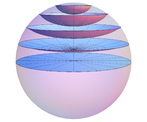
Figure 2: The extremal surfaces in $AdS_{4}$ space-time for various choices of $\theta_{0}$.

Parametrizing the extremal surface with the coordinates $\phi$ and $r$, the induced metric turns out to be diagonal with elements

$${\gamma_{rr}} =\frac{{{{\sin}^{2}}{\theta_{0}}}}{{{r^{2}}\left({1+\frac{1}{{{r^{2}}}}}\right)\left[{1-\left({1+\frac{1}{{{r^{2}}}}}\right){{\cos}^{2}}{\theta_{0}}}\right]}},$$ (2.19)

$${\gamma_{\varphi\varphi}} ={r^{2}}\left[{1-\left({1+\frac{1}{{{r^{2}}}}}\right){{\cos}^{2}}{\theta_{0}}}\right].$$ (2.20)

The determinant of the induced metric is $\gamma={\sin}^{2}{\theta_{0}}/(1+1/r^{2})$ and the area follows from equation (2.8),

$$A^{\rm extr}=2\pi\mathop{\lim}\limits_{r\to\infty}\left({r\sin{\theta_{0}}-1}\right).$$ (2.21)

The first term is the divergent “area law” term, while the second one is universal independent of the UV cutoff [30, 31].

2.4 Perturbations of Entanglement Entropy

The area functional (2.8) depends on the background metric $g$ as well as on the embedding variables $X$, and, of course, it also depends implicitly on the entangling curve $\partial A$ curving the region $A$ in the boundary field theory. Perturbations of the bulk metric induce changes of the minimal surface. The variation of its area is given in general by

$$\delta A^{\rm extr}={\left.{\frac{{\delta A^{\rm extr}\left({g,X}\right)}}{{\delta g}}}\right|_{g={g_{0}},\,X={X_{0}}}}\delta g+{\left.{\frac{{\delta A^{\rm extr}\left({g,X}\right)}}{{\delta X}}}\right|_{g={g_{0}},\,X={X_{0}}}}\delta X$$ (2.23)

as both the metric and the embedding equations of the extremal surface vary around their unperturbed values $g_{0}$ and $X_{0}$.

When the perturbation obeys Dirichlet boundary conditions, the region $A$ and its boundary $\partial A$ remain fixed. Then, the second term vanishes, as the original surface described by equations $X_{0}$ extremizes the area functional with the given loop $\partial A$. When the metric perturbations satisfy general boundary conditions, computing the variation of the area of the minimal surface is more subtle. For this, we suppose that the boundary loop $\partial A$ specifying the extremal surface is determined by a set of parameters $b$, which may also vary as metric perturbations are turned on. Then, the area functional has the particular form

$$A^{\rm extr}=A^{\rm extr}\left({g,X\left({g,b}\right)}\right)$$ (2.24)

and its variation breaks down as follows,

$$\delta A^{\rm extr}={\left.{\frac{{\delta A^{\rm extr}\left({g,X}\right)}}{{\delta g}}}\right|_{g={g_{0}},\,X={X_{0}}}}\delta g\\ +{\left.{\frac{{\delta A^{\rm extr}\left({g,X}\right)}}{{\delta X}}}\right|_{g={g_{0}},\,X={X_{0}}}}{\left.{\frac{{\delta X\left({g,b}\right)}}{{\delta g}}}\right|_{g={g_{0}},\,b={b_{0}}}}\delta g\\ +{\left.{\frac{{\delta A^{\rm extr}\left({g,X}\right)}}{{\delta X}}}\right|_{g={g_{0}},\,X={X_{0}}}}{\left.{\frac{{\partial X\left({g,b}\right)}}{{\partial b}}}\right|_{g={g_{0}},\,b={b_{0}}}}\delta b.$$ (2.25)

The second term vanishes, as it corresponds to the variation of the area for variations of the extremal surface with a fixed boundary that is provided by the entangling loop $\partial A$. The last term can be simplified if one considers the area as functional of the metric as well as the parameters $b$ specifying the entangling loop. As a result, the total variation of the area takes the form

$$\begin{split}\delta A^{\rm extr}&={\left.{\frac{{\delta A^{\rm extr}\left({g,X}\right)}}{{\delta g}}}\right|_{g={g_{0}},\,X={X_{0}}}}\delta g+{\left.{\frac{{\partial A^{\rm extr}\left({g,b}\right)}}{{\partial b}}}\right|_{g={g_{0}},\,b={b_{0}}}}\delta b\\ &:=\delta{A_{g}^{\rm extr}}+\delta{A_{b}^{\rm extr}}\,,\end{split}$$ (2.26)

hereby defining the individual contributions $\delta{A_{g}^{\rm extr}}$ and $\delta{A_{b}^{\rm extr}}$.

The first term follows by varying the relation (2.8) and the result is written in terms of the unperturbed induced metric $\gamma_{0}$ and $\delta\gamma_{ab}$ as

$$\delta A_{g}^{\rm extr}=\frac{1}{2}\int{{d^{2}}\sigma\sqrt{{\gamma_{0}}}{\left(\gamma_{0}\right)}^{ab}\delta{\gamma_{ab}}}\,,$$ (2.27)

where

$${{\left(\gamma_{0}\right)}_{ab}}={\left(g_{0}\right)}_{\mu\nu}\frac{{\partial{X_{0}}^{\mu}\left(\sigma\right)}}{{\partial{\sigma^{a}}}}\frac{{\partial{X_{0}}^{\nu}\left(\sigma\right)}}{{\partial{\sigma^{b}}}},$$ (2.28)

$$\delta{\gamma_{ab}}=\delta{g_{\mu\nu}}\frac{{\partial{X_{0}}^{\mu}\left(\sigma\right)}}{{\partial{\sigma^{a}}}}\frac{{\partial{X_{0}}^{\nu}\left(\sigma\right)}}{{\partial{\sigma^{b}}}}.$$ (2.29)

The second term can be easily calculated for polar caps, which only depends on a single parameter $b$ that is taken to be $\theta_{0}$. Then, $\delta{A_{b}^{\rm extr}}$ follows by varying the relation (2.21) with respect to the cap parameter $\theta_{0}$.

The individual terms $\delta{A_{g}^{\rm extr}}$ and $\delta{A_{b}^{\rm extr}}$ will be explicitly computed later for small perturbations of the $AdS_{4}$ metric satisfying the linearized Einstein equations with general boundary conditions.

2.5 Modular Hamiltonian for a Polar Cap Region

Unlike the Ryu-Takayanagi formula for expressing the entanglement entropy in terms of the bulk gravitational theory, there is no similar expression for the modular Hamiltonian. In general, the modular Hamiltonian is a non-local operator and there is no way to this day to find an expression for the modular Hamiltonian for a general boundary state and region $A$. In some cases, however, the modular Hamiltonian generates a geometric flow leading to a local expression.

Such an example is provided by taking a disk region $A$ of radius $R$ in a Minkowski space boundary [18], in which case the modular flow in the Cauchy development of the disk can be connected with the modular flow in Rindler space through a conformal transformation; the details are provided in B. Then, the modular Hamiltonian is expressed in terms of the holographic energy-momentum tensor and a conformal Killing vector that leaves invariant the entangling curve $\partial A$ and its causal development, as

$$\delta E_{A}=\int_{C}{d{\Sigma^{\mu}}{\mathcal{T}_{\mu\nu}}{\zeta^{\nu}}},$$ (2.30)

where $C$ is a space-like surface with boundary $\partial A$ and ${d{\Sigma^{\mu}}}$ is the differential volume form on $C$ [17]. If $C$ is selected to be a constant time slice, it will coincide with the region $A$. For a disk in Minkowski space, this conformal Killing vector $\zeta$ is a linear combination of the Killing vectors corresponding to the time translation and a special conformal transformation; it is selected so that $\zeta$ vanishes on $\partial A$ and its causal development.

Using the coordinate transformation (2.13), the conformal Killing vector in question takes the following form in global coordinates (for more details see A),

$$\zeta=\frac{2\pi}{{\sin{\theta_{0}}}}\left[{\left({\cos\left({t-{t_{0}}}\right)\cos\theta-\cos{\theta_{0}}}\right){\partial_{t}}-\sin\left({t-{t_{0}}}\right)\sin\theta{\partial_{\theta}}}\right],$$ (2.31)

which indeed satisfies the conformal Killing vector equation

$${\nabla_{\mu}}{\zeta_{\nu}}+{\nabla_{\nu}}{\zeta_{\mu}}-\frac{2}{d}{g_{\mu\nu}}{\nabla_{\lambda}}{\zeta^{\lambda}}=0$$ (2.32)

and at the same time vanishes at the entangling surface $\theta=\theta_{0}$ and $t=t_{0}$. The conformal Killing vector $\zeta$ is the boundary limit of a conformal Killing vector field $\xi$ in the bulk,

$$\xi=\frac{2\pi}{{\sin{\theta_{0}}}}\left[{\left({\frac{{r\cos\theta\cos\left({t-{t_{0}}}\right)}}{{\sqrt{{r^{2}}+1}}}-\cos{\theta_{0}}}\right){\partial_{t}}}\phantom{\frac{{\sqrt{{r^{2}}+1}\sin\theta\sin\left({t-{t_{0}}}\right)}}{r}}\right.\\ \left.{+\sqrt{{r^{2}}+1}\cos\theta\sin\left({t-{t_{0}}}\right){\partial_{r}}-\frac{{\sqrt{{r^{2}}+1}\sin\theta\sin\left({t-{t_{0}}}\right)}}{r}{\partial_{\theta}}}\right],$$ (2.33)

which also vanishes at the entangling surface.

Note in passing that if one considers generalized theories of gravity (i.e., higher derivative corrections) an appropriate generalization of Ryu-Takayanagi conjecture will be required. Such generalizations can be obtained through the Iyer-Wald theorem that involves bifurcate Killing horizons generated by the conformal Killing vector $\xi$ given by (2.33) [20].

Formula (2.30) can be evaluated for any space-like surface with boundary identical to the entangling surface. Selecting the $t=t_{0}$ surface and using the specific form of the Killing vector (2.31), the modular Hamiltonian for the polar cap region $\theta\leq\theta_{0}$ is written as

$$\delta E_{A}=\frac{4\pi^{2}}{{\sin{\theta_{0}}}}\int_{0}^{{\theta_{0}}}{d\theta\sin\theta\left({\cos\theta-\cos{\theta_{0}}}\right){\mathcal{T}_{tt}}}.$$ (2.34)

This completes the presentation of the general formulae for the quantities of interest. In section 4 $\delta E$ will be calculated and compared to $\delta S$ for all different kinds of $AdS_{4}$ perturbations satisfying general boundary conditions.

3 Linearized Gravity in AdS₄

Now we come to the theory of gravitational perturbations of $AdS_{4}$ space-time, allowing for general boundary conditions. It is convenient to split the perturbations into two complementary sets with opposite parity and reduce the linearized Einstein equations to an affective Schrödinger problem, which is exactly solvable. Then, we write down the holographic energy-momentum tensor for all such perturbations, which will be used later. The material we present here is based on the discussion found in [26] (but see also [27] for an overview of the subject) and references therein.

3.1 Linear AdS₄ Perturbations

We consider Einstein gravity in four space-time dimensions with negative cosmological constant $\Lambda$,

$${R_{\mu\nu}}=\Lambda{g_{\mu\nu}}\,.$$ (3.1)

$AdS_{4}$ is the maximally symmetric solution whose metric takes the following form in spherical coordinates,

$$d{s^{2}}=-f\left(r\right)d{t^{2}}+\frac{{d{r^{2}}}}{{f\left(r\right)}}+{r^{2}}\left({d{\theta^{2}}+{{\sin}^{2}}\theta d{\varphi^{2}}}\right),$$ (3.2)

where

$$f\left(r\right)=1-\frac{\Lambda}{3}{r^{2}}.$$ (3.3)

We set the AdS scale $\sqrt{-3/\Lambda}$ equal to one to simplify the presentation. For later use, we define the tortoise coordinate $x$ as

$$dx=\frac{{dr}}{{f\left(r\right)}}\,,$$ (3.4)

which is given explicitly as

$$r=\tan x\,.$$ (3.5)

The tortoise coordinate is an angular variable ranging from $0$ to $\pi/2$ as $r$ varies from $0$ to $\infty$.

Next, we consider linear perturbations around the $AdS_{4}$ metric (3.2) satisfying Einstein’s equations. The gravitational perturbations fall in two complementary classes with opposite parity, namely axial and polar perturbations. Without loss of generality we restrict attention to axially symmetric deformations, which are described in terms of Legendre polynomials $P_{l}\left(\cos\theta\right)$ instead of more general spherical harmonics $Y_{l}^{m}\left(\theta,\phi\right)$.

Axial Perturbations

The metric perturbations of this class are parametrized by two functions ${h_{0}}\left(r\right)$ and ${h_{1}}\left(r\right)$ as follows,

$$d{s^{2}}=-f\left(r\right)d{t^{2}}+\frac{{d{r^{2}}}}{{f\left(r\right)}}+{r^{2}}\left({d{\theta^{2}}+{{\sin}^{2}}\theta d{\varphi^{2}}}\right)\\ +2{e^{-i\omega t}}\sin\theta\frac{{d{P_{l}}\left({\cos\theta}\right)}}{{d\theta}}\left({{h_{0}}\left(r\right)dt+{h_{1}}\left(r\right)dr}\right)d\varphi,$$ (3.6)

up to reparametrizations. It turns out that Einstein’s equations are equivalent to the effective Schrödinger problem with respect to the tortoise coordinate,

$$-\frac{{{d^{2}}{\Psi_{{\rm{ax}}}}\left(x\right)}}{{d{x^{2}}}}+\frac{{l\left({l+1}\right)}}{{{{\sin}^{2}}x}}{\Psi_{{\rm{ax}}}}\left(x\right)={\omega^{2}}{\Psi_{{\rm{ax}}}}\left(x\right),$$ (3.7)

where the functions ${h_{0}}\left(r\right)$ and ${h_{1}}\left(r\right)$ are expressed in terms of the solutions as

$${h_{0}}\left(x\right) =\frac{i}{\omega}\frac{d}{{dx}}\left({\tan x\,{\Psi_{{\rm{ax}}}}\left(x\right)}\right),$$ (3.8)

$${h_{1}}\left(x\right) =\sin x\cos x\,{\Psi_{{\rm{ax}}}}\left(x\right).$$ (3.9)

Polar Perturbations

The metric perturbations of this class are parametrized by three functions ${H_{0}}\left(r\right)$, ${H_{1}}\left(r\right)$ and $K\left(r\right)$ as follows,

$$d{s^{2}}=-f\left(r\right)d{t^{2}}+\frac{{d{r^{2}}}}{{f\left(r\right)}}+{r^{2}}\left({d{\theta^{2}}+{{\sin}^{2}}\theta d{\varphi^{2}}}\right)\\ +{e^{-i\omega t}}{P_{l}}\left({\cos\theta}\right)\left[{{H_{0}}\left(r\right)\left({f\left(r\right)d{t^{2}}+\frac{{d{r^{2}}}}{{f\left(r\right)}}}\right)}\right.\\ \left.\phantom{\left({f\left(r\right)d{t^{2}}+\frac{{d{r^{2}}}}{{f\left(r\right)}}}\right)}{+\,2{H_{1}}\left(r\right)dtdr+K\left(r\right){r^{2}}\left({d{\theta^{2}}+{{\sin}^{2}}\theta d{\varphi^{2}}}\right)}\right],$$ (3.10)

up to reparametrizations. Similarly to the previous case, Einstein’s equations for polar perturbations turn out to be equivalent to the effective Schrödinger problem with respect to the tortoise coordinate,

$$-\frac{{{d^{2}}{\Psi_{\rm{pol}}}\left(x\right)}}{{d{x^{2}}}}+\frac{{l\left({l+1}\right)}}{{{{\sin}^{2}}x}}{\Psi_{\rm{pol}}}\left(x\right)={\omega^{2}}{\Psi_{\rm{pol}}}\left(x\right),$$ (3.11)

which is identical to the one describing the axial perturbations. The functions ${H_{0}}\left(r\right)$, ${H_{1}}\left(r\right)$ and $K\left(r\right)$ are expressed in terms of the solutions of the effective Schrödinger problem as

$${H_{0}}\left(x\right) =\left({\frac{{l\left({l+1}\right)}}{2}\cot x-{\omega^{2}}\sin x\cos x+{{\cos}^{2}x}\,\frac{d}{{dx}}}\right){\Psi_{\rm{pol}}}\left(x\right),$$ (3.12)

$${H_{1}}\left(x\right) =-i\omega\cos x\frac{d}{{dx}}\left({\sin x\,{\Psi_{\rm{pol}}}\left(x\right)}\right),$$ (3.13)

$$K\left(x\right) =\left({\frac{{l\left({l+1}\right)}}{2}\cot x+\frac{d}{{dx}}}\right){\Psi_{\rm{pol}}}\left(x\right).$$ (3.14)

Thus, the spectrum and the eigen-functions of the operator $-d^{2}/dx^{2}+l(l+1)/{\rm sin}^{2}x$ in the closed interval $x\in[0,\,\pi/2]$ completely determine the gravitational perturbations of $AdS_{4}$ space-time. The general solution of the linearized Einstein equations is written as linear combination of the axial and polar solutions.

3.2 Boundary Conditions

The solution of effective Schrödinger problem can be expressed in terms of hypergeometric functions. The normalizable solution, which vanishes at $r=0$, is

$$\Psi\left(x\right)=\cos x{\sin^{l+1}}x\,F\left({\frac{1}{2}\left({l+2+\omega}\right),\,\frac{1}{2}\left({l+2-\omega}\right);\,l+\frac{3}{2};\,{{\sin}^{2}}x}\right).$$ (3.15)

The other independent solution of the effective Schrödinger problem is

$$\Psi\left(x\right)=\frac{{\cos x}}{{{{\sin}^{l}}x}}\,F\left({\frac{1}{2}\left({-l+1+\omega}\right),\,\frac{1}{2}\left({-l+1-\omega}\right);\,\frac{1}{2}-l;\,{{\sin}^{2}}x}\right),$$ (3.16)

but it diverges as $r\to 0$ and is not normalizable.

The boundary conditions as $r\to\infty$ can be systematically described by expanding the normalizable solutions in powers of $1/r$, as

$${\Psi}={I_{0}}+\frac{{{I_{1}}}}{r}+\frac{{{I_{2}}}}{{{r^{2}}}}+\frac{{{I_{3}}}}{{{r^{3}}}}+\ldots.$$ (3.17)

Using properties of the hypergeometric functions, it turns out that $I_{0}$ and $I_{1}$ are expressed in terms of Gamma-functions as

$$I_{0} = \Gamma^{-1}\left({1\over 2}(l+2+\omega)\right)\Gamma^{-1}\left({1\over 2}(l+2-\omega)\right)\,,$$ (3.18)

$$I_{1} = -2\Gamma^{-1}\left({1\over 2}(l+1+\omega)\right)\Gamma^{-1}\left({1\over 2}(l+1-\omega)\right)\,.$$ (3.19)

The coefficients of all other terms are expressed in terms of $I_{0}$ and $I_{1}$, but the details do not really matter. We only note here, for later use, that

$${I_{2}}=\frac{{{I_{0}}}}{2}\left({l\left({l+1}\right)-{\omega^{2}}}\right).$$ (3.20)

The boundary conditions imposed as $r\to\infty$ are solely described in terms $I_{0}$ and $I_{1}$, since

$$I_{0}=\Psi(r=\infty)\,,~{}~{}~{}~{}~{}~{}I_{1}=-{d\Psi\over dx}(r=\infty)\,.$$ (3.21)

Thus, solutions, characterized by $I_{0}=0$ obey Dirichlet boundary conditions for the effective Schrödinger problem, while solutions characterized by $I_{1}=0$ obey Neumann boundary conditions. Solutions with $I_{0}$ and $I_{1}$ taking more general values correspond to more general (mixed) boundary conditions determined by the ratio $I_{0}/I_{1}$. In the following, we will denote by $I_{k}$ the coefficients of the large $r$ expansion of $\Psi(r)$ associated to axial perturbations and $J_{k}$ for the polar perturbations, for distinction.

For given boundary conditions, the spectrum is discrete; for example, for Dirichlet boundary conditions we find

$$\omega_{D}=\pm\left(2n+l+2\right),$$ (3.22)

whereas for Neumann boundary conditions the spectrum is

$$\omega_{N}=\pm\left(2n+l+1\right).$$ (3.23)

More general boundary conditions give rise to intermediate (generally not equidistant) frequencies. In all cases, the spectrum is implicitly determined by ratios of Gamma-functions fixed by the ratio $I_{0}/I_{1}$ or $J_{0}/J_{1}$.

3.3 The Holographic Energy-Momentum Tensor

The energy-momentum tensor is divergent in asymptotic AdS spaces and appropriate renormalization is required to make sense of it, using counter-terms. Here, we summarize the results of holographic renormalization [33, 34, 35, 36] for the boundary space-time metric and the corresponding energy-momentum tensor for gravitational perturbations of $AdS_{4}$ space-time satisfying general boundary conditions, following [26]. Thus, we have per sector the following results, setting Newton’s constant $G_{N}=1$:

Axial Perturbations

The boundary metric after conformal rescaling takes the form

$$d{s^{2}}=-d{t^{2}}+\left({d{\theta^{2}}+{{\sin}^{2}}\theta d{\varphi^{2}}}\right)+\frac{{2i{I_{0}}}}{\omega}{e^{-i\omega t}}\sin\theta\frac{{d{P_{l}}\left({\cos\theta}\right)}}{{d\theta}}dtd\varphi\,,$$ (3.24)

whereas the non-vanishing components of the energy momentum tensor for small perturbations are

$$8\pi{\mathcal{T}_{t\varphi}} =-\frac{i}{{2\omega}}\left({l-1}\right)\left({l+2}\right){I_{1}}{e^{-i\omega t}}\sin\theta\frac{{d{P_{l}}\left({\cos\theta}\right)}}{{d\theta}}\,,$$ (3.25)

$$8\pi{\mathcal{T}_{\theta\varphi}} =-\frac{1}{2}{I_{1}}{e^{-i\omega t}}\sin\theta\left[{l\left({l+1}\right){P_{l}}\left({\cos\theta}\right)+2\cot\theta\frac{{d{P_{l}}\left({\cos\theta}\right)}}{{d\theta}}}\right]\,.$$ (3.26)

Polar Perturbations

In this sector, the boundary metric after conformal rescaling takes the form

$$d{s^{2}}=-d{t^{2}}+\left({1-{J_{1}}{e^{-i\omega t}}{P_{l}}\left({\cos\theta}\right)}\right)\left({d{\theta^{2}}+{{\sin}^{2}}\theta d{\varphi^{2}}}\right),$$ (3.27)

whereas the non-vanishing components of the energy-momentum tensor for the corresponding small perturbations are

$$8\pi{\mathcal{T}_{tt}} =\frac{1}{4}\left({l-1}\right)l\left({l+1}\right)\left({l+2}\right){J_{0}}{e^{-i\omega t}}{P_{l}}\left({\cos\theta}\right),$$ (3.28)

$$8\pi{\mathcal{T}_{\theta\theta}} =-\frac{1}{4}l\left({l+1}\right)\left({1-{\omega^{2}}}\right){J_{0}}{e^{-i\omega t}}{P_{l}}\left({\cos\theta}\right)$$

$$-\frac{1}{4}\left({l\left({l+1}\right)-2{\omega^{2}}}\right){J_{0}}{e^{-i\omega t}}\cot\theta\frac{{d{P_{l}}\left({\cos\theta}\right)}}{{d\theta}}\,,$$ (3.29)

$$8\pi{\mathcal{T}_{\varphi\varphi}} =\frac{1}{4}l\left({l+1}\right)\left({l\left({l+1}\right)-1-{\omega^{2}}}\right){J_{0}}{e^{-i\omega t}}{\sin^{2}}\theta{P_{l}}\left({\cos\theta}\right)$$

$$+\frac{1}{4}\left({l\left({l+1}\right)-2{\omega^{2}}}\right){J_{0}}{e^{-i\omega t}}\sin\theta\cos\theta\frac{{d{P_{l}}\left({\cos\theta}\right)}}{{d\theta}}\,,$$ (3.30)

$$8\pi{\mathcal{T}_{t\theta}} =\frac{i}{4}\omega\left({l-1}\right)\left({l+2}\right){J_{0}}{e^{-i\omega t}}\frac{{d{P_{l}}\left({\cos\theta}\right)}}{{d\theta}}\,.$$ (3.31)

In all cases, the energy-momentum tensor is traceless and covariantly conserved,

$${\mathcal{T}_{a}}^{a}=0\,,~{}~{}~{}~{}~{}~{}~{}\nabla_{a}\mathcal{T}^{ab}=0$$ (3.32)

with respect to the boundary metric, as required on general grounds.

Equations (3.24) and (3.27) imply that for axial perturbations Dirichlet boundary conditions for the effective Schrödinger problem correspond to Dirichlet conditions for the metric, while for polar perturbations Neumann boundary conditions for the effective Schrodinger problem correspond to Dirichlet conditions for the metric. These results will be particularly useful while computing the modular Hamiltonian as an appropriately weighted integral of the energy density for all kind of perturbations. It can already be seen that $\delta E$ always vanishes for axial perturbations, since ${\mathcal{T}_{tt}}=0$ irrespective of boundary conditions, whereas $\delta E$ does not vanish for polar perturbations satisfying boundary conditions other than $J_{0}=0$.

4 Entanglement Entropy for Gravitational Perturbations

We are now in position to compute holographically the variation of the entanglement entropy and the modular Hamiltonian for gravitational perturbations of $AdS_{4}$ space-time satisfying general boundary conditions. First, we compute the variation of the area of the extremal surface emanating from the loop $\partial A$, as $\delta A^{\rm extr}=\delta A_{g}^{\rm extr}+\delta A_{b}^{\rm extr}$, then we compute $\delta E$, and, finally, we compare the results with the first law of thermodynamics for the entanglement entropy, $\delta S=\delta E$. We find that the deformations of the entangling curve $\partial A$ should be isoperimetric, when the boundary conditions of the metric allow for fluctuating geometries on the boundary of $AdS_{4}$ for, otherwise, the first law of thermodynamics would not be realized holographically. Our results generalize earlier work on the subject, going from Dirichlet to more general boundary conditions for the metric.

4.1 Calculation of $\delta A_{g}^{\rm extr}$

First, we work out the contribution $\delta A_{g}^{\rm extr}$ to the variation of the area of the minimal surface. Naturally, we consider the effect of axial and polar perturbations separately.

Axial Perturbations

For axial perturbations, the variation of the induced metric on the minimal surface, which is generally given by equation (2.29), turns out to be

$$\delta{\gamma_{rr}} =\delta{\gamma_{\varphi\varphi}}=0\,,$$ (4.1)

$$\delta{\gamma_{r\varphi}} =\delta{g_{r\varphi}}={\left.{h_{1}}\left(r\right){e^{-i\omega t_{0}}}\sin\theta\frac{\partial}{{\partial\theta}}{P_{l}}\left({\cos\theta}\right)\right|}_{\theta=\arccos\left({\cos{\theta_{0}}\sqrt{1+\frac{1}{{{r^{2}}}}}}\right)}$$ (4.2)

and so the corresponding variation of the area, given by equation (2.27), is

$$\delta{A_{g}^{\rm extr}}=0\,.$$ (4.3)

Polar Perturbations

For polar perturbations, the variation of the induced metric (2.29) turns out to be

$$\delta{\gamma_{rr}}=\delta{g_{rr}}+{\left({\frac{{d\theta}}{{dr}}}\right)^{2}}\delta{g_{\theta\theta}}$$

$$=\frac{1}{{1+{r^{2}}}}\left({{H_{0}}\left(r\right)+\frac{{{{\cos}^{2}}\theta_{0}K\left(r\right)}}{{{r^{2}}\left({1-\left({1+\frac{1}{{{r^{2}}}}}\right){{\cos}^{2}}\theta_{0}}\right)}}}\right){e^{-i\omega t_{0}}}{P_{l}}\left({\cos{\theta_{0}}\sqrt{1+\frac{1}{{{r^{2}}}}}}\right),$$ (4.4)

$$\delta{\gamma_{\varphi\varphi}}=\delta{g_{\varphi\varphi}}={r^{2}}\left({1-\left({1+\frac{1}{{{r^{2}}}}}\right){{\cos}^{2}}\theta_{0}}\right)K\left(r\right){e^{-i\omega t_{0}}}{P_{l}}\left({\cos{\theta_{0}}\sqrt{1+\frac{1}{{{r^{2}}}}}}\right),$$ (4.5)

$$\delta{\gamma_{r\varphi}}=0\,.$$ (4.6)

Then, using equations (2.19), (2.20) and (2.27), we find after some algebra that

$$\delta{A_{g}^{\rm extr}}=\pi\int_{\cot{\theta_{0}}}^{\infty}{dr\frac{{\sin{\theta_{0}}}}{{\sqrt{\left({1+\frac{1}{{{r^{2}}}}}\right)}}}\left[{\left({{H_{0}}\left(r\right)+K\left(r\right)}\right)}\phantom{\frac{1}{{{r^{2}}{{\tan}^{2}}{\theta_{0}}}}}\right.}\\ \left.{+\frac{1}{{{r^{2}}{{\tan}^{2}}{\theta_{0}}}}\left({K\left(r\right)-{H_{0}}\left(r\right)}\right)}\right]{e^{-i\omega t_{0}}}{P_{l}}\left({\cos{\theta_{0}}\sqrt{1+\frac{1}{{{r^{2}}}}}}\right).$$ (4.7)

Trading $r$ with the tortoise coordinate $x$ and expressing $H_{0}$ and $K$ in terms of the $\Psi_{\rm pol}$, as given by equations (3.12) and (3.14), we obtain

$$\delta{A_{g}^{\rm extr}}=\pi\int_{\frac{\pi}{2}-{\theta_{0}}}^{\frac{\pi}{2}}{dx\frac{{\sin{\theta_{0}}}}{{\cos x}}\left[{l\left({l+1}\right){\Psi_{\rm{pol}}}-{\left({1-\frac{{{{\cos}^{2}}x}}{{{{\sin}^{2}}{\theta_{0}}}}}\right)}{\omega^{2}}{\Psi_{\rm{pol}}}}\right.}\\ \left.{+\tan x\left({1+\frac{{{{\cos}^{2}}x}}{{{{\sin}^{2}}{\theta_{0}}}}}\right)\frac{{d{\Psi_{\rm{pol}}}}}{{dx}}}\right]{e^{-i\omega t_{0}}}{P_{l}}\left({\frac{{\cos{\theta_{0}}}}{{\sin x}}}\right).$$ (4.8)

The effective Schrödinger problem (3.11) can be used further to eliminate $\omega$, leading to the following expression,

$$\delta{A_{g}^{\rm extr}}=\pi\int_{\frac{\pi}{2}-{\theta_{0}}}^{\frac{\pi}{2}}{dx\left[{\frac{d}{{dx}}\left[{\left({\frac{{\sin{\theta_{0}}}}{{\cos x}}-\frac{{\cos x}}{{\sin{\theta_{0}}}}}\right)\frac{{d{\Psi_{\rm{pol}}}}}{{dx}}}\right]}\right.}\\ \left.{+l\left({l+1}\right)\frac{{\cos{\theta_{0}}\cot x}}{{\tan{\theta_{0}}\sin x}}\,{\Psi_{\rm{pol}}}}\right]{e^{-i\omega t_{0}}}{P_{l}}\left({\frac{{\cos{\theta_{0}}}}{{\sin x}}}\right).$$ (4.9)

It is convenient at this point to employ the following identities among Legendre polynomials,

$$\frac{d}{{d\xi}}\left({{P_{l+1}}\left(\xi\right)-{P_{l-1}}\left(\xi\right)}\right) =\left({2l+1}\right){P_{l}}\left(\xi\right),$$ (4.10)

$$\frac{d}{{d\xi}}{P_{l}}\left(\xi\right) =\frac{{l\left({l+1}\right)}}{{2l+1}}\frac{1}{{{\xi^{2}}-1}}\left({{P_{l+1}}\left(\xi\right)-{P_{l-1}}\left(\xi\right)}\right),$$ (4.11)

to perform integration by parts and get

$$\delta{A_{g}^{\rm extr}}=\pi{e^{-i\omega t_{0}}}\left[{\left({\frac{{\sin{\theta_{0}}}}{{\cos x}}-\frac{{\cos x}}{{\sin{\theta_{0}}}}}\right)\frac{{d{\Psi_{\rm{pol}}}}}{{dx}}\,{P_{l}}\left({\frac{{\cos{\theta_{0}}}}{{\sin x}}}\right)}\right]_{\frac{\pi}{2}-{\theta_{0}}}^{\frac{\pi}{2}}\\ -\pi{e^{-i\omega t_{0}}}\left[{\cot{\theta_{0}}\,\frac{{l\left({l+1}\right)}}{{2l+1}}\left({{P_{l+1}}\left({\frac{{\cos{\theta_{0}}}}{{\sin x}}}\right)-{P_{l-1}}\left({\frac{{\cos{\theta_{0}}}}{{\sin x}}}\right)}\right)}{\Psi_{\rm{pol}}}\right]_{\frac{\pi}{2}-{\theta_{0}}}^{\frac{\pi}{2}}.$$ (4.12)

The contribution from the end-point $x=\frac{\pi}{2}-\theta_{0}$ vanishes for both bracketed terms, and, thus, the result is

$$\delta{A_{g}^{\rm extr}}=\pi{e^{-i\omega t_{0}}}\mathop{\lim}\limits_{x\to\frac{\pi}{2}}\left[{\frac{{\sin{\theta_{0}}}}{{\cos x}}\frac{{d{\Psi_{\rm{pol}}}}}{{dx}}\,{P_{l}}\left({\cos{\theta_{0}}}\right)}\right.\\ \left.{-\cot{\theta_{0}}\,\frac{{l\left({l+1}\right)}}{{2l+1}}\left({{P_{l+1}}\left({\cos{\theta_{0}}}\right)-{P_{l-1}}\left({\cos{\theta_{0}}}\right)}\right)}\,{\Psi_{\rm{pol}}}\right].$$ (4.13)

Going back to the coordinate $r$ and using the asymptotic expansion of the Schrödinger wave-functions (3.17) together with equation (3.20), we arrive at the final expression

$$\delta{A_{g}^{\rm extr}}=-\pi{e^{-i\omega t_{0}}}\left[{\mathop{\lim}\limits_{r\to\infty}\left({r{J_{1}}+{J_{0}}\left({l\left({l+1}\right)-{\omega^{2}}}\right)}\right)\sin{\theta_{0}}\,{P_{l}}\left({\cos{\theta_{0}}}\right)}\phantom{\frac{{l\left({l+1}\right)}}{{2l+1}}}\right.\\ \left.{+\cot{\theta_{0}}\,\frac{{l\left({l+1}\right)}}{{2l+1}}{J_{0}}\left({{P_{l+1}}\left({\cos{\theta_{0}}}\right)-{P_{l-1}}\left({\cos{\theta_{0}}}\right)}\right)}\right].$$ (4.14)

Note that $\delta{A_{g}^{\rm extr}}$ is divergent when the perturbations of the metric do not satisfy Dirichlet boundary conditions, $J_{1}\neq 0$.

4.2 Calculation of $\delta A_{b}^{\rm extr}$

Since we are considering axially symmetric perturbations of the bulk metric, the deformations of the entangling curve are taken to be independent of the angular coordinate $\phi$ to conform with the symmetry. Thus, the variations of the parameter $\theta_{0}$ in the polar cap are taken to be independent of $\phi$, i.e.,

$$\theta_{0}\left(t\right)=\theta_{0}+\delta\theta\left(t\right).$$ (4.15)

Consequently, $\delta{A_{b}^{\rm extr}}$ can be derived directly by varying (2.21) with respect to $\theta_{0}$, leading to the following result

$$\delta{A_{b}^{\rm extr}}=2\pi\mathop{\lim}\limits_{r\to\infty}r\cos{\theta_{0}}\,\delta\theta\left(t_{0}\right)$$ (4.16)

for all kind of metric perturbations.

Note that $\delta A_{b}^{\rm extr}$ also appears to be divergent on general grounds. It is important to see how these divergences combine with those appearing in $\delta A_{g}^{\rm extr}$ to form $\delta A^{\rm extr}$.

4.3 Net Variation of the Entanglement Entropy

Summing up the two contributions, we obtain the net variation of the area of the minimal surface, $\delta A^{\rm extr}$, and, hence, the variation of entanglement entropy, $\delta S_{A}$. We present the result for axial and polar perturbations,

setting Newton’s constant $G_{N}=1$. Thus, for axial perturbations, we have

$$\delta S_{A}^{{\rm{axial}}}=\frac{\pi}{2}\mathop{\lim}\limits_{r\to\infty}r\cos{\theta_{0}}\,\delta{\theta}^{{\rm{axial}}}\left(t_{0}\right),$$ (4.17)

whereas for polar perturbations the result reads

$$\delta S_{A}^{{\rm{polar}}}=-\frac{\pi}{4}{e^{-i\omega t_{0}}}\left[{\mathop{\lim}\limits_{r\to\infty}\left({r{J_{1}}+{J_{0}}\left({l\left({l+1}\right)-{\omega^{2}}}\right)}\right)\sin{\theta_{0}}\,{P_{l}}\left({\cos{\theta_{0}}}\right)}\phantom{\frac{{l\left({l+1}\right)}}{{2l+1}}}\right.\\ \left.{+\cot{\theta_{0}}\,\frac{{l\left({l+1}\right)}}{{2l+1}}{J_{0}}\left({{P_{l+1}}\left({\cos{\theta_{0}}}\right)-{P_{l-1}}\left({\cos{\theta_{0}}}\right)}\right)}\right]\\ +\frac{\pi}{2}\mathop{\lim}\limits_{r\to\infty}r\cos{\theta_{0}}\,\delta{\theta}^{{\rm{polar}}}\left(t_{0}\right).$$ (4.18)

The variance of the entropy appears to be divergent, which is unphysical. Specific conditions should be imposed on $\delta{\theta}^{{\rm{polar}}}(t_{0})$ to make them cancel, but these will be discussed later, while comparing $\delta S_{A}$ with $\delta E_{A}$, together with their geometric meaning.

4.4 Modular Hamiltonian for Gravitational Perturbations

Next, we compute the variation of the modular Hamiltonian by specializing formula (2.34) to axial and polar perturbations satisfying general boundary conditions. As before, Newton’s constant is set equal to 1.

Axial Perturbations

Since $\mathcal{T}_{tt}=0$ for the axial perturbations, we immediately obtain

$$\delta E_{A}^{{\rm{axial}}}=0$$ (4.19)

in all cases, irrespective of boundary conditions.

Polar Perturbations

For polar perturbations with $J_{0}\neq 0$, the component $\mathcal{T}_{tt}$ of the holographic energy-momentum tensor does not vanish, and, hence, the corresponding variance of the modular Hamiltonian differs from zero.

First, substituting the expression (3.28) for $\mathcal{T}_{tt}$ into equation (2.34), yields the following expression for the variance of the modular Hamiltonian,

$$\delta E_{A}^{{\rm{polar}}}=\frac{\pi\left({l-1}\right)l\left({l+1}\right)\left({l+2}\right)}{{8\sin{\theta_{0}}}}{J_{0}}{e^{-i\omega{t_{0}}}}\int_{0}^{{\theta_{0}}}{d\theta\sin\theta\left({\cos\theta-\cos{\theta_{0}}}\right){P_{l}}\left({\cos\theta}\right)}\,.$$ (4.20)

Then, we perform integration by parts and make use of formula (4.10) twice to find

$$\delta E_{A}^{{\rm{polar}}}=\frac{\pi}{{8\sin{\theta_{0}}}}\frac{{\left({l-1}\right)l\left({l+1}\right)\left({l+2}\right)}}{{2l+1}}{J_{0}}{e^{-i\omega{t_{0}}}}\\ \times\left[{\frac{{{P_{l+2}}\left({\cos{\theta_{0}}}\right)}}{{2l+3}}+\frac{{{P_{l-2}}\left({\cos{\theta_{0}}}\right)}}{{2l-1}}-\frac{{2\left({2l+1}\right){P_{l}}\left({\cos{\theta_{0}}}\right)}}{{\left({2l-1}\right)\left({2l+3}\right)}}}\right].$$ (4.21)

Next, using the following identity of Legendre polynomials,

$$\left({l+1}\right){P_{l+1}}\left(\xi\right)+l{P_{l-1}}\left(\xi\right)=\left({2l+1}\right)\xi\,{P_{l}}\left(\xi\right)$$ (4.22)

to eliminate $P_{l-2}$ and $P_{l+2}$, we arrive at the expression

$$\delta E_{A}^{{\rm{polar}}}=\frac{\pi}{{8\sin{\theta_{0}}}}\frac{{\left({l-1}\right)l\left({l+1}\right)\left({l+2}\right)}}{{2l+1}}{J_{0}}{e^{-i\omega{t_{0}}}}\\ \times\left[{\cos{\theta_{0}}\left({\frac{{{P_{l+1}}\left({\cos{\theta_{0}}}\right)}}{{l+2}}+\frac{{{P_{l-1}}\left({\cos{\theta_{0}}}\right)}}{{l-1}}}\right)-\frac{{\left({2l+1}\right){P_{l}}\left({\cos{\theta_{0}}}\right)}}{{\left({l-1}\right)\left({l+2}\right)}}}\right],$$ (4.23)

which can be conveniently rewritten as

$$\delta E_{A}^{{\rm{polar}}}=\frac{\pi}{{8\sin{\theta_{0}}}}\frac{{\left({l-1}\right)l\left({l+1}\right)\left({l+2}\right)}}{{2l+1}}{J_{0}}{e^{-i\omega{t_{0}}}}\\ \times\left[{\frac{{\cos{\theta_{0}}}}{{\left({l-1}\right)\left({l+2}\right)}}\left({\left({l+1}\right){P_{l+1}}\left({\cos{\theta_{0}}}\right)+l{P_{l-1}}\left({\cos{\theta_{0}}}\right)}\right)}\right.\\ \left.{-\frac{{2\cos{\theta_{0}}}}{{\left({l-1}\right)\left({l+2}\right)}}\left({{P_{l+1}}\left({\cos{\theta_{0}}}\right)-{P_{l-1}}\left({\cos{\theta_{0}}}\right)}\right)-\frac{{\left({2l+1}\right){P_{l}}\left({\cos{\theta_{0}}}\right)}}{{\left({l-1}\right)\left({l+2}\right)}}}\right].$$ (4.24)

Using once more the identity (4.22) yields the final result,

$$\delta E_{A}^{{\rm{polar}}}=-\frac{\pi}{{4}}{e^{-i\omega t_{0}}}\left[{\frac{1}{2}{J_{0}}\,l\left({l+1}\right)\sin{\theta_{0}}{P_{l}}\left({\cos{\theta_{0}}}\right)}\right.\\ \left.{+\cot{\theta_{0}}\,\frac{{l\left({l+1}\right)}}{{2l+1}}{J_{0}}\left({{P_{l+1}}\left({\cos{\theta_{0}}}\right)-{P_{l-1}}\left({\cos{\theta_{0}}}\right)}\right)}\right].$$ (4.25)

We see that in all cases the variance of the modular Hamiltonian is finite.

4.5 Comparison with First Law of Thermodynamics

The first law of thermodynamics $\delta S=\delta E$ for the entanglement entropy and the modular Hamiltonian is a tautology from the point of view of the boundary theory. Its realization through the Ryu-Takayanagi formula (2.7) and the holographic energy-momentum tensor is not automatic, but it is a consistency check of the whole scheme. Comparing the results derived above, we find that $\delta S_{A}=\delta E_{A}$ for any polar cap region A, provided that the entangling curve at the boundary also deforms, where appropriate, in a certain way. The boundary is not held fixed when general boundary conditions are imposed on the metric, and, thus, the polar cap region $A$ and the entangling curve $\partial A$ also vary. Thus, $\delta\theta(t_{0})$ should be adjusted accordingly to achieve agreement with the first law of thermodynamics. As will be seen shortly this requirement has natural geometric interpretation. It also gets rid of the divergences appearing in the computation of $\delta S_{A}$.

Axial Perturbations

First, we consider the case of axial perturbations and compare the expressions (4.17) for $\delta S_{A}$ and (4.19) for $\delta E_{A}$. The first law is realized holographically provided that

$$\delta{\theta}^{{\rm{axial}}}\left(t_{0}\right)=0$$ (4.26)

irrespective of boundary conditions. Thus, axial perturbations do not require adjustment of the polar cap region.

A way to understand this is to consider the boundary metric of the perturbed $AdS_{4}$ space-time, prior to conformal scaling, and work out the two-dimensional induced metric on the corresponding polar cap region. For axial perturbations it reads

$${ds^{2}}_{\rm{axial}}={r^{2}}\left({d{\theta^{2}}+{{\sin}^{2}}\theta d{\varphi^{2}}}\right).$$ (4.27)

The polar cap is placed on a round sphere that remains inert to perturbations irrespective of boundary conditions.

Polar Perturbations

Next, we consider the case of polar perturbations and compare the corresponding expressions (4.18) for $\delta S_{A}$ and (4.25) for $\delta E_{A}$. The first law of thermodynamics for entanglement entropy is realized holographically provided that the entangling curve in the polar cap region varies according to the equation

$$\delta{\theta}^{{\rm{polar}}}\left(t_{0}\right)=\frac{1}{2}{e^{-i\omega t_{0}}}\left[{{J_{1}}+\frac{{J_{0}}}{{r}}\left({\frac{1}{2}l\left({l+1}\right)-{\omega^{2}}}\right)}\right]\tan{\theta_{0}}\,{P_{l}}\left({\cos{\theta_{0}}}\right).$$ (4.28)

This also takes care of the unphysical divergences appearing in $\delta S_{A}$. Note at this end that a subleading term proportional to $J_{0}$ is included in the variation $\delta{\theta}^{{\rm{polar}}}(t_{0})$; it contributes a finite term to $\delta S_{A}$ which should also be removed to match it with $\delta E_{A}$.

In this case, perturbations of the bulk metric require adjusting the entangling curve in the boundary. To understand what is happening, let us consider the boundary metric of the perturbed $AdS_{4}$ space-time, prior to conformal scaling, and work out the two-dimensional induced metric on the corresponding polar cap region $A$. For polar perturbations, the induced metric on the spherical slices of the boundary is

$${ds^{2}}_{\rm{polar}}={r^{2}}\left({1+K\left(r\right){e^{-i\omega t}}{P_{l}}\left({\cos{\theta}}\right)}\right)\left({d{\theta^{2}}+{{\sin}^{2}}\theta d{\varphi^{2}}}\right),$$ (4.29)

where $K(r)$ is the radial function appearing in the general parametrization (3.10) of the bulk space metric. The asymptotic form for $K\left(r\right)$ follows from the large $r$ expansion of the Schrödinger wave function $\Psi_{\rm pol}$, via equation (3.14), and it reads

$$K\left(r\right)=-{J_{1}}-\frac{{J_{0}}}{{r}}\left({\frac{1}{2}l\left({l+1}\right)-{\omega^{2}}}\right)+\mathcal{O}\left({\frac{1}{{{r^{2}}}}}\right).$$ (4.30)

It implies, in particular, that the condition (4.28) on $\delta{\theta}^{{\rm{polar}}}\left(t_{0}\right)$ takes the following equivalent form

$$\delta{\theta}^{{\rm{polar}}}\left(t_{0}\right)=-\frac{1}{2}{e^{-i\omega t_{0}}}K(r)\tan{\theta_{0}}\,{P_{l}}\left({\cos{\theta_{0}}}\right)$$ (4.31)

up to irrelevant subleading terms.

The deformation of the entangling curve is such that its line element is inert to the perturbation. Using the spherical metric (4.29), we find that the induced line element of the boundary curve of a polar cap region with parameter $\theta$ is

$$dl=\mathop{\lim}\limits_{r\to\infty}\sqrt{{g_{\varphi\varphi}}}\,d\varphi=\mathop{\lim}\limits_{r\to\infty}\left({1+\frac{1}{2}K\left(r\right){e^{-i\omega t}}{P_{l}}\left({\cos\theta}\right)}\right)r\sin\theta\,d\varphi\,.$$ (4.32)

Here, we also take the large $r$ limit as the computations take place on the boundary of space-time, prior to rescaling. Setting $\theta=\theta_{0}+\delta\theta(t_{0})$, where $\delta\theta(t_{0})$ is provided by (4.31), we have to linear order that

$$\left({1+\frac{1}{2}K\left(r\right){e^{-i\omega t_{0}}}{P_{l}}\left({\cos({\theta_{0}}}+\delta\theta\left(t_{0}\right))\right)}\right)r\sin\left({{\theta_{0}}+\delta{\theta}\left(t_{0}\right)}\right)=$$

$$\left({1+\frac{1}{2}K\left(r\right){e^{-i\omega t_{0}}}{P_{l}}\left({\cos{\theta_{0}}}\right)}\right)r\sin\left({{\theta_{0}}+\delta{\theta}\left(t_{0}\right)}\right)=r\sin{\theta_{0}}+\mathcal{O}\left(\frac{1}{r}\right).$$ (4.33)

Thus, although the polar cap region and its boundary undergo perturbations, the line element of the entangling curve remains constant,

$$dl=\mathop{\lim}\limits_{r\to\infty}r\sin\theta_{0}\,d\varphi\,.$$ (4.34)

Summarizing, we see that for all kind of gravitational perturbations of $AdS_{4}$ space-time (axial or polar) and for all kind of boundary conditions, the holographic realization of the first law of thermodynamics requires that the line element of the entangling curve remains invariant. Region $A$, whose entanglement entropy is provided by formula (2.7), deforms with time in such a way that the line element of the entangling curve remains constant. This requirement also takes care of the divergencies that otherwise would have inflicted the variance of the entanglement entropy. Since the first law of thermodynamics is trivially valid from the CFT point of view, the above statement should be viewed as addendum to Ryu-Takayanagi prescription.

Although the laws of entanglement thermodynamics are not yet completely understood, it has been shown that for spherical regions the reduced density matrix $\rho_{A}$ is identical to a thermal density matrix with effective inverse temperature equal to the perimeter of the entangling circular curve [18]. Through this connection, our results can be thought to provide the holographic interpretation of an isothermal process of entanglement thermodynamics.

An interesting question arises by comparing our calculation to previous ones [19, 20]. In those papers, the first law of thermodynamics for entanglement was realized holographically using gravitational perturbations satisfying Dirichlet boundary conditions, without making reference to the contribution $\delta A_{b}^{\rm extr}$. In our case, even for Dirichlet boundary conditions for the polar perturbations of the metric, $J_{1}=0$, $\delta A_{b}^{\rm extr}$ is non-vanishing. Its contribution is absolutely necessary for validating the first law of thermodynamics for entanglement. The resolution to this ostensible contradiction is that each one of the terms arising in $\delta A_{g}^{\rm extr}$ and $\delta A_{b}^{\rm extr}$ depend on the choice of coordinates, but their net sum is, in fact, coordinate independent when the line element of the entangling curve remains constant. The variation $\delta A_{b}^{\rm extr}$ vanishes for Dirichlet boundary conditions only in some coordinate systems, which include the Fefferman-Graham coordinates used in references [19, 20]. More technical details about this issue are provided in C.

The demand for isometric deformations of the entangling curve is also strongly connected with renormalization issues of the entanglement entropy. In odd dimensional conformal field theories, as in our case, the finite contribution to the entanglement entropy can be contaminated by the divergent terms, using alternative definitions of the UV cutoff scale $L$. This issue has already been noticed in the literature [18]. The universal constant term can be isolated using an appropriate renormalized entanglement entropy, which in $2+1$ conformal field theories (and at least for special choices of the entangling curve) takes the form [37]

$${\tilde{S}_{EE}}:={S_{EE}}-\frac{{\partial{S_{EE}}}}{{\partial\,{\rm{L}}\left({\partial A}\right)}}\,{\rm{L}}\left({\partial A}\right),$$ (4.35)

where ${\rm{L}}\left({\partial A}\right)$ is the length of the entangling curve, resolving the above issue. This is also in agreement, via the Ryu-Takayanagi conjecture, with the definition of renormalized area in the bulk theory, provided by Graham and Witten [38]; in that work the same contamination arises from the divergent terms, resulting in a specific choice of radial coordinate to cure the problem. When the metric perturbations of $AdS_{4}$ are taken in the form (3.6) or (3.10), the corresponding radial coordinate $r$ does not belong to that special class, calling for a renormalized definition of holographic entanglement entropy, as in equation (4.35). In this language, the term $\delta A_{g}^{\rm extr}$ corresponds to the variation of $S_{EE}$, whereas the term $\delta A_{b}^{\rm extr}$ corresponds to the variation of the counter-term. Then, as it is implied by our results, the inclusion of the counter-term is equivalent to the statement that the unrenormalized entanglement entropy, which is provided by the Ryu-Takayanagi formula (2.7), is computed for a region $A$ bounded by an entangling curve that deforms isometrically.

5 Electric-Magnetic Duality for Entanglement Entropy

In this section, we review briefly the electric-magnetic duality exhibited by linearized gravity, together with its holographic manifestation, following [26], and examine the implications to entanglement entropy.

5.1 Energy-Momentum/Cotton Tensor Duality

Linearized gravity around maximally symmetric backgrounds exhibits a rank-2 generalization of electric-magnetic duality in four space-time dimensions [22, 23]. It is best described in terms of the Weyl tensor $C_{\mu\nu\rho\sigma}$ and its dual counterpart,

$${{\tilde{C}}_{\mu\nu\rho\sigma}}=\frac{1}{2}{\varepsilon_{\mu\nu}}^{\kappa\lambda}{C_{\kappa\lambda\rho\sigma}},$$ (5.1)

as follows:

The Weyl tensor vanishes identically for maximally symmetric backgrounds, $Mink_{4}$, $dS_{4}$ or $AdS_{4}$, which are solutions of the full non-linear Einstein equations with cosmological constant $\Lambda$. Linearized gravity around the maximally symmetric solution, whose choice depends upon the sign of the $\Lambda$, exhibits a symmetry under the interchange of the electric and magnetic components of the corresponding Weyl tensor. At the level of equations, it amounts to exchanging the role of the linearized field equations and the Bianchi identities. Two metric perturbations $\delta\tilde{g}_{\mu\nu}$ and $\delta g_{\mu\nu}$ are said to be dual to each other if

$${{\tilde{C}}_{\mu\nu\rho\sigma}}\left(g\right)={C_{\mu\nu\rho\sigma}}\left({\tilde{g}}\right),$$ (5.2)

so that the electric components of the one Weyl tensor are the magnetic components of the other and vice-versa. Although these relations are highly non-local, they are naturally resolved by decomposing the gravitational perturbations into two distinct classes of opposite parity, namely axial and polar perturbations. It turns out that

$${\delta{\tilde{g}}^{{\rm{polar}}}}={\delta g^{{\rm{axial}}}}\,,~{}~{}~{}~{}~{}~{}{\delta{\tilde{g}}^{{\rm{axial}}}}={\delta g^{{\rm{polar}}}}\,,$$ (5.3)

provided that the solutions of the corresponding effective Schrödinger problems are interrelated as

$${{\tilde{\Psi}}_{\rm{pol}}}=-\frac{{2i}}{\omega}{\Psi_{{\rm{ax}}}}\,,~{}~{}~{}~{}~{}~{}{{\tilde{\Psi}}_{{\rm{ax}}}}=\frac{{i\omega}}{2}{\Psi_{\rm{pol}}}\,.$$ (5.4)

Since the Schrödinger problems of the axial and polar perturbations are identical, though the precise form of the effective potential depends on the cosmological constant $\Lambda$, the relation among $\tilde{\Psi}$ and $\Psi$ enforces the two classes of perturbations to have the same frequency $\omega$ and the same boundary conditions at spatial infinity.

Specializing the discussion to gravitational perturbations of $AdS_{4}$ space-time, which is the subject of the present work, one finds that electric-magnetic duality has a holographic manifestation [24, 25, 26, 27]. Quite remarkably, the holographic energy-momentum tensor $\mathcal{T}_{ab}$ and the Cotton tensor $\mathcal{C}_{ab}$ of the metric at the boundary of space-time follow from the electric and magnetic components of the bulk Weyl tensor (with respect to the radial ADM decomposition of the metric) as

$$8\pi{\mathcal{T}_{ab}} =-\mathop{\lim}\limits_{r\to\infty}{r^{3}}{C_{arbr}}\,,$$ (5.5)

$${\mathcal{C}_{ab}} =\mathop{\lim}\limits_{r\to\infty}{r^{3}}{{\tilde{C}}_{arbr}}\,.$$ (5.6)

The Cotton tensor is traceless, symmetric and covariantly conserved, as for the energy-momentum tensor, and it measures the deviations of the boundary metric from conformal flatness due to the boundary conditions one imposes on the perturbations of the metric. The last equations are general and applicable to the full non-linear regime of $AdS_{4}$ gravity, but when specialized to the linearized theory they give rise to the so called energy-momentum/Cotton tensor duality that is resolved in sectors as

$$8\pi{\mathcal{T}_{ab}^{{\rm{polar}}}}={\mathcal{C}_{ab}^{{\rm{axial}}}},$$ (5.7)

$$8\pi{\mathcal{T}_{ab}^{{\rm{axial}}}}={\mathcal{C}_{ab}^{{\rm{polar}}}}.$$ (5.8)

5.2 Duality for Entanglement Entropy

The extremal surface $A^{\rm extr}$, whose area provides the entanglement entropy, is defined with respect to a given bulk metric $g$ for a given boundary region. Let us define ${{\tilde{A}}^{{\rm{extr}}}}$ as the extremal surface taken with respect to the dual metric ${\tilde{g}}$, following (5.2),

$${{\tilde{A}}^{{\rm{extr}}}}\left(g\right)={A^{{\rm{extr}}}}\left({\tilde{g}}\right).$$ (5.9)

The corresponding entanglement entropy is taken to be

$${{\tilde{S}}_{A}}={1\over 4}\,{\rm{Area}}\left({{{\tilde{A}}^{{\rm{extr}}}}}\right)\,.$$ (5.10)

Since the unperturbed $AdS_{4}$ space is self dual, ${{\tilde{g}}_{\rm AdS}}={g_{\rm AdS}}$, the unperturbed extremal surface is also self-dual. The variation of the dual entanglement entropy for axial and polar perturbations, which are dual to each other, can be calculated in the same way as the variation of entanglement entropy. As a direct consequence of equations (5.3), we obtain

$$\delta{{\tilde{S}}^{{\rm{axial}}}} =\delta{S^{{\rm{polar}}}},$$ (5.11)

$$\delta{{\tilde{S}}^{{\rm{polar}}}} =\delta{S^{{\rm{axial}}}}.$$ (5.12)

Similarly, one can define the variation of the dual modular Hamiltonian using the Cotton tensor of the original boundary metric, as

$$\delta\tilde{E}=\frac{1}{8\pi}\int_{C}{d{\Sigma^{\mu}}{\mathcal{C}_{\mu\nu}}{\zeta^{\nu}}}.$$ (5.13)

As direct consequence of equations (5.7) and (5.8), it turns out that

$$\delta{{\tilde{E}}^{{\rm{axial}}}} =\delta{E^{{\rm{polar}}}},$$ (5.14)

$$\delta{{\tilde{E}}^{{\rm{polar}}}} =\delta{E^{{\rm{axial}}}}.$$ (5.15)

It is true that $\delta S=\delta E$ for all kind of perturbations, and, thus, it is also true that

$$\delta\tilde{S}=\delta\tilde{E}\,,$$ (5.16)

showing that the first law of thermodynamics for entanglement is self-dual under gravitational duality.

Note in this context that the boundary metric is not identical to the dual boundary metric, since the duality transformation interchanges Dirichlet and Neumann boundary conditions for the metric (it only preserves the boundary conditions of the effective Schrödinger problems). Since the line element of the entangling curve remains inert to perturbations, the entangling curve is not identical to the dual entangling curve. Likewise, the polar cap region $A$ is not the same as its dual counterpart $\tilde{A}$. These differences should be taken into account in the definitions of the dual thermodynamic quantities above.

6 Conclusions and Discussion

In this paper we studied the variation of the entanglement entropy and the expectation value of the modular Hamiltonian for small gravitational perturbations of $AdS_{4}$ space-time satisfying general boundary conditions. We found that the first law of thermodynamics for entanglement is realized holographically through the Ryu-Takayanagi formula, provided that the line element of the entangling curve on the boundary remains constant, hereby generalizing previous results on the subject. It should be viewed as addendum to the Ryu-Takayanagi prescription. In this context, we also noted that the perimeter of the entangling curve is the “area” appearing in the “area law” term for entanglement entropy. Thus, our demand that the line element of the entangling curve remains constant is equivalent to the statement that the “area law” term is inert to metric perturbations for all different kind of boundary conditions. In turn, this appears to be equivalent to using a certain renormalized form for the holographic entanglement entropy.

Although our presentation is technically limited to metric perturbations and entangling curves that are axially symmetric, choosing polar cap regions with circular boundary, we expect it to generalize in the absence of axial symmetry. It will be interesting to see how exactly this happens.

We also examined the implications of electric-magnetic duality of linearized gravity for the entanglement entropy and the associated first law of thermodynamics. We defined a dual entanglement entropy and a dual modular Hamiltonian and found that they also satisfy the first law of thermodynamics for appropriately related dual regions $A$ and $\tilde{A}$ at the boundary of $AdS_{4}$. These results too can be thought to provide an additional consistency check of the Ryu-Takayanagi conjecture.

Typically, electric-magnetic duality connects the dual degrees of freedom of the theory in a non-trivial and non-local way. In the absence of excitations, it reduces to a trivial local relation, but this is not any more so in the presence of excitations. If one defines the entanglement entropy in a region by tracing out the degrees of freedom in the complement, the same degrees of freedom will correspond to a different region in the dual description. Thus, the dual entanglement entropy should be defined for a different entangling curve. Our results, showing that the holographic realization of the first law of thermodynamics is achieved only when the line element of the entangling curve remains constant, are in accord with the different boundary conditions satisfied by dual gravitational excitations so that the dual boundary metrics differ.

It would be interesting to see if such considerations can also be applied to other backgrounds such as $AdS_{4}$ black holes. Perturbations of black-holes exhibit a duality relation which is best described in terms of supersymmetric partner potentials for the effective Schrödinger problems of the axial and polar sectors. Although this duality has no direct interpretation in terms of the electric and magnetic components of the Weyl tensor in the bulk, as in $AdS_{4}$ space-time, it has holographic manifestation as energy-momentum/Cotton tensor duality for the hydrodynamic modes of black holes [39]. We hope to address the related thermal effects of black holes elsewhere.

Appendix A Useful relations in Poincaré and Spherical Coordinates

It is known that in Poincaré coordinates, the extremal surface corresponding to a disk region with radius $R$ centered at $\left(x_{0},y_{0}\right)$ is given by the “hemisphere”,

$$\begin{split}{\left({x-{x_{0}}}\right)^{2}}+{\left({y-{y_{0}}}\right)^{2}}+{z^{2}}&={R^{2}},\\ \tau&={\tau_{0}}\,.\end{split}$$ (A.1)

Changing to global spherical coordinates, using the coordinate transformation (2.13), the surface (A.1) takes the form,

$$\begin{split}\cos\theta&=\cos{\theta_{0}}\sqrt{1+\frac{1}{{{r^{2}}}}}\,,\\ t&={t_{0}}\,,\end{split}$$ (A.2)

where $\theta_{0}$ and $t_{0}$ are given by

$$\cos{\theta_{0}} =\frac{{1-{R^{2}}+{\tau_{0}}^{2}}}{{\sqrt{\left[{{{\left({R+{\tau_{0}}}\right)}^{2}}+1}\right]\left[{{{\left({R-{\tau_{0}}}\right)}^{2}}+1}\right]}}}\,,$$ (A.3)

$$\cos{t_{0}} =\frac{{1+{R^{2}}-{\tau_{0}}^{2}}}{{\sqrt{\left[{{{\left({R+{\tau_{0}}}\right)}^{2}}+1}\right]\left[{{{\left({R-{\tau_{0}}}\right)}^{2}}+1}\right]}}}\,.$$ (A.4)

To express the variation of the modular Hamiltonian for the polar cap region in spherical coordinates, we needed the expression for the conformal Killing vector in the boundary, $\zeta$, that leaves the entangling curve invariant. This is the limit of a conformal Killing vector in the bulk, $\xi$, which in Poincaré coordinates and with the appropriate normalization takes the following form [20],

$$\xi=\frac{\pi}{R}\left[{\left({{R^{2}}-{z^{2}}-{{\left({\tau-{\tau_{0}}}\right)}^{2}}-{{\left({x-{x_{0}}}\right)}^{2}}-{{\left({y-{y_{0}}}\right)}^{2}}}\right){\partial_{\tau}}}\right.\\ \left.\phantom{\left({{{\left({y-{y_{0}}}\right)}^{2}}}\right)}{-2\left({\tau-{\tau_{0}}}\right)\left({z{\partial_{z}}+\left({x-{x_{0}}}\right){\partial_{x}}+\left({y-{y_{0}}}\right){\partial_{y}}}\right)}\right].$$ (A.5)

In our analysis, the entangling curve is taken to be axially symmetric, as for the metric perturbations. This selects $x_{0}=y_{0}=0$, so that the center of the disc is placed at the north pole. Furthermore, since the $AdS_{4}$ metric is static, we may choose a specific instant of time to simplify the calculations. The choice ${\tau_{0}}=\sqrt{1+{R^{2}}}$ implies that

$$\tan{\theta_{0}} =R\,,$$ (A.6)

$$\cos{t_{0}} =0\,.$$ (A.7)

At that instant, the conformal Killing vector $\xi$ in the bulk takes the form

$$\xi=\frac{\pi}{R}\left[{\left({{R^{2}}-{z^{2}}-{{\left({\tau-\sqrt{1+{R^{2}}}}\right)}^{2}}-{x^{2}}-{y^{2}}}\right){\partial_{\tau}}}\right.\\ \left.\phantom{\left({{{\left({\tau-\sqrt{1+{R^{2}}}}\right)}^{2}}}\right)}{-2\left({\tau-\sqrt{1+{R^{2}}}}\right)\left({z{\partial_{z}}+x{\partial_{x}}+y{\partial_{y}}}\right)}\right].$$ (A.8)

Converting to spherical coordinates by the transformation (2.13), we find

$$\xi=\frac{{2\pi\sqrt{1+{R^{2}}}}}{R}\left[{\left({\frac{{r\cos\theta\sin t}}{{\sqrt{1+{r^{2}}}}}-\frac{1}{{\sqrt{1+{R^{2}}}}}}\right){\partial_{t}}}\phantom{\frac{{\sqrt{1+{r^{2}}}}}{r}}\right.\\ \left.{-\sqrt{1+{r^{2}}}\cos\theta\cos t{\partial_{r}}+\frac{{\sqrt{1+{r^{2}}}\sin\theta\cos t}}{r}{\partial_{\theta}}}\right],$$ (A.9)

which can be rewritten as

$$\xi=\frac{{2\pi}}{{\sin{\theta_{0}}}}\left[{\left({\frac{{r\cos\theta\cos\left({t-{t_{0}}}\right)}}{{\sqrt{1+{r^{2}}}}}-\cos{\theta_{0}}}\right){\partial_{t}}}\phantom{\frac{{\sqrt{1+{r^{2}}}\left({t-{t_{0}}}\right)}}{r}}\right.\\ \left.{+\sqrt{1+{r^{2}}}\cos\theta\sin\left({t-{t_{0}}}\right){\partial_{r}}-\frac{{\sqrt{1+{r^{2}}}\sin\theta\sin\left({t-{t_{0}}}\right)}}{r}{\partial_{\theta}}}\right].$$ (A.10)

Then, the boundary limit of this expression provides the desired conformal Killing vector $\zeta$, which reads

$$\zeta=\frac{2\pi}{{\sin{\theta_{0}}}}\left[{\left({\cos\left({t-{t_{0}}}\right)\cos\theta-\cos{\theta_{0}}}\right){\partial_{t}}-\sin\left({t-{t_{0}}}\right)\sin\theta{\partial_{\theta}}}\right]$$ (A.11)

and is used to compute the variation of the modular Hamiltonian in section 2.5.

Appendix B The Modular Flow for a Disc in Minkowski Space-time

It is not known how to express the modular Hamiltonian for a general region and state. This difficulty stems from the fact that, in general, the modular Hamiltonian is a non-local operator. Exceptionally, in some cases, the modular Hamiltonian generates a geometric flow and can be expressed as a local operator. Here, we outline how this is actually realized for a disk region in Minkowski space-time.

The modular Hamiltonian defines a symmetry of the system. More specifically, the symmetry group is provided by the unitary operators $U\left(s\right)=e^{-iHs}$ and it is called the modular group,

$$\mathrm{Tr}\left({\rho U\left(s\right)OU\left({-s}\right)}\right)=\mathrm{Tr}\left({\rho{\rho^{is}}O{\rho^{-is}}}\right)=\mathrm{Tr}\left({{\rho^{-is}}\rho{\rho^{is}}O}\right)=\mathrm{Tr}\left({\rho O}\right).$$ (B.1)

We define $O\left(s\right)=U\left(s\right)OU\left(-s\right)$. When the modular Hamiltonian is not a local operator, this flow is non-local.

If one extends the modular group to imaginary parameters, there will be a periodicity relation in imaginary time,

$$\mathrm{Tr}\left({\rho{O_{1}}\left(i\right){O_{2}}}\right)=\mathrm{Tr}\left({\rho U\left(i\right){O_{1}}U\left({-i}\right){O_{2}}}\right)=\mathrm{Tr}\left({\rho{\rho^{-1}}{O_{1}}\rho{O_{2}}}\right)=\mathrm{Tr}\left({\rho{O_{2}}{O_{1}}}\right).$$ (B.2)

Thus, the state $\rho$ is thermal with respect to the time evolution of the modular symmetry with temperature $T=1$.

Let us consider Minkowski space-time in coordinates $X^{\mu}$. The Rindler space $\mathcal{R}$ is defined as the causal development of the half plane $X^{1}<0$. The causal development of a region $A$ is the set of space-time points whose causal space-time curves necessarily cross region $A$. The modular transformations map the local operators $O\left(X\right)$ in Rindler space $\mathcal{R}$ to themselves. More specifically, the modular flow acts on the coordinates as follows,

$${X^{\pm}}\left(s\right)={X^{\pm}}{e^{\pm 2\pi s}},~{}~{}~{}~{}~{}~{}{X^{i}}\left(s\right)={X^{i}},$$ (B.3)

where ${X^{\pm}}={X^{1}}\pm{X^{0}}$ and the Latin indices $i$ run from 2 to $d-1$.

The modular Hamiltonian for $\mathcal{R}$ can be calculated explicitly. Transforming to the usual Rindler coordinates ${X^{\pm}}=z{e^{\pm\tau/R}}$, the metric becomes

$$d{s^{2}}=-\frac{{{z^{2}}}}{{{R^{2}}}}d{\tau^{2}}+d{z^{2}}+d{X^{i}}d{X^{i}},$$ (B.4)

corresponding to a thermal state with temperature $T=1/2\pi R$. Thus, the density matrix can be expressed as

$${\rho_{\mathcal{R}}}=\frac{{{e^{-2\pi R{H_{\tau}}}}}}{{\mathrm{Tr}{e^{-2\pi R{H_{\tau}}}}}}$$ (B.5)

with modular Hamiltonian

$${H_{\mathcal{R}}}=2\pi R{H_{\tau}}+\log\mathrm{Tr}{e^{-2\pi R{H_{\tau}}}}.$$ (B.6)

The result for Rindler space can be subsequently used to obtain the modular Hamiltonian for a disc $D$ of radius $R$. The conformal transformation

$${x^{\mu}}=\frac{{{X^{\mu}}-{X_{\nu}}{X^{\nu}}{C^{\mu}}}}{{1-2{X_{\kappa}}{C^{\kappa}}+{X_{\rho}}{X^{\rho}}{C_{\sigma}}{C^{\sigma}}}}+\frac{{{C^{\mu}}}}{{2{C_{\lambda}}{C^{\lambda}}}}\,,$$ (B.7)

with

$${C^{\mu}}=\left({0\,,\,\frac{1}{{2R}}\,,\,0\,,\ldots,\,0}\right)$$ (B.8)

yields

$${\eta_{\mu\nu}}d{X^{\mu}}d{X^{\nu}}={\Omega^{2}}{\eta_{\mu\nu}}d{x^{\mu}}d{x^{\nu}}$$ (B.9)

with

$$\Omega=1-2{X_{\kappa}}{C^{\kappa}}+{X_{\rho}}{X^{\rho}}{C_{\sigma}}{C^{\sigma}}.$$ (B.10)

Letting $r=\sqrt{\left({x^{1}}\right)^{2}+\ldots+\left({x^{d-1}}\right)^{2}}$ and $t=x^{0}$, we see that this conformal transformation maps the half plane $X^{1}\leq 0$ to the disk $D$, $r\leq R$, and the Rindler space $X^{\pm}\leq 0$ to the causal development of the disk $\mathcal{D}$, $x^{\pm}\leq R$, where $x^{\pm}=r\pm t$. For later use, we express the new radial coordinate as

$$r=\frac{1}{\Omega}\sqrt{{X^{i}}{X^{i}}+{{\left({R-\frac{{{X_{\nu}}{X^{\nu}}}}{{4R}}}\right)}^{2}}}.$$ (B.11)

Also, the inverse coordinate transformation is

$${X^{\mu}}=\Omega\left({{x^{\mu}}+2{x_{\nu}}{x^{\nu}}{C^{\mu}}}\right)-\frac{{{C^{\mu}}}}{{{C_{\lambda}}{C^{\lambda}}}}\,,$$ (B.12)

where

$$\Omega={\left({\frac{1}{4}+{C_{\kappa}}{x^{\kappa}}+{C_{\lambda}}{C^{\lambda}}{x_{\nu}}{x^{\nu}}}\right)^{-1}}.$$ (B.13)

We want to determine the form of the modular flow in the new coordinate system. For this purpose, we first make use of equations (B.3) and (B.12) to find the flow of the conformal factor $\Omega$,

$$\begin{split}\Omega\left(s\right)&=1-\frac{{{X^{1}}\left(s\right)}}{R}+\frac{{{X_{\nu}}{X^{\nu}}}}{{4{R^{2}}}}\\ &=\Omega-\frac{1}{R}\left[{\left({\cosh 2\pi s-1}\right){X^{1}}+\sinh 2\pi s{X^{0}}}\right]\\ &=\Omega\left({\frac{1}{2}\frac{{{R^{2}}+{r^{2}}-{t^{2}}}}{{{R^{2}}}}+\frac{1}{2}\cosh 2\pi s\frac{{{t^{2}}+{R^{2}}-{r^{2}}}}{{{R^{2}}}}-\sinh 2\pi s\frac{t}{R}}\right)\\ &=\frac{\Omega}{{{R^{2}}}}\left({R\cosh\pi s-{x^{+}}\sinh\pi s}\right)\left({R\cosh\pi s+{x^{-}}\sinh\pi s}\right).\end{split}$$ (B.14)

The radial coordinate $r$, which is given by equation (B.11), also flows through its dependence on the conformal factor,

$$r\left(s\right)=\frac{1}{{\Omega\left(s\right)}}\sqrt{{X^{i}}{X^{i}}+{{\left({R-\frac{{{X_{\nu}}{X^{\nu}}}}{{4R}}}\right)}^{2}}}=\frac{\Omega}{{\Omega\left(s\right)}}\,r\,.$$ (B.15)

Similarly, the modular flow of the new time coordinate can be expressed as

$$\begin{split}t\left(s\right)&=\frac{{{X^{0}}\left(s\right)}}{{\Omega\left(s\right)}}=\frac{{\cosh 2\pi s{X^{0}}+\sinh 2\pi s{X^{1}}}}{{\Omega\left(s\right)}}\\ &=\frac{\Omega}{{\Omega\left(s\right)}}\,R\left({\cosh 2\pi s\frac{t}{R}-\frac{1}{2}\sinh 2\pi s\frac{{{t^{2}}+{R^{2}}-{r^{2}}}}{{{R^{2}}}}}\right),\end{split}$$ (B.16)

which in turn implies that

$$\begin{split}\frac{{\Omega\left(s\right)}}{\Omega}\,{x^{\pm}}\left(s\right)&=r\pm R\left({\cosh 2\pi s\frac{t}{R}-\frac{1}{2}\sinh 2\pi s\frac{{{t^{2}}+{R^{2}}-{r^{2}}}}{{{R^{2}}}}}\right)\\ &=\frac{1}{R}\left({R\cosh\pi s\pm{x^{\mp}}\sinh\pi s}\right)\left({{x^{\pm}}\cosh\pi s\mp R\sinh\pi s}\right).\end{split}$$ (B.17)

Finally, we obtain

$${x^{\pm}}\left(s\right)=R\frac{{{x^{\pm}}\cosh\pi s\mp R\sinh\pi s}}{{R\cosh\pi s\mp{x^{\pm}}\sinh\pi s}}=R\frac{{\left({R+{x^{\pm}}}\right)-\left({R-{x^{\pm}}}\right){e^{\mp 2\pi s}}}}{{\left({R+{x^{\pm}}}\right)+\left({R-{x^{\pm}}}\right){e^{\mp 2\pi s}}}}.$$ (B.18)

The modular flow in the new coordinates yields by differentiation

$${\left.{\frac{{\partial{x^{\pm}}\left(s\right)}}{{\partial s}}}\right|_{s=0}} =\pm\pi\frac{{{R^{2}}-{x^{\pm}}^{2}}}{R}\,,$$ (B.19)

$${\left.{\frac{{\partial r\left(s\right)}}{{\partial s}}}\right|_{s=0}} =-2\pi\frac{{rt}}{R}\,,$$ (B.20)

$${\left.{\frac{{\partial t\left(s\right)}}{{\partial s}}}\right|_{s=0}} =\pi\frac{{{R^{2}}-{r^{2}}-{t^{2}}}}{R}\,,$$ (B.21)

clarifying the action of the modular Hamiltonian on local operators in the new coordinates. Restricting attention to the time slice $t=0$, one recovers the usual expression for the modular Hamiltonian for a disk of radius $R$ [18], namely

$$H_{D}=2\pi\int{{d^{d-1}}x\,\frac{{{R^{2}}-{r^{2}}}}{{2R}}\,{\mathcal{T}^{00}}}.$$ (B.22)

Appendix C Coordinate Dependence of Subleading Terms in $\delta A_{g}^{\rm extr}$, $\delta A_{b}^{\rm extr}$

The individual contributions to the variation of the area, $\delta A_{g}^{\rm extr}$ and $\delta A_{b}^{\rm extr}$, which appear in section 4, are coordinate dependent, unlike their sum which is coordinate independent when the line element of the entangling curve remains constant. Furthermore, the term $\delta A_{b}^{\rm extr}$ only vanishes for Dirichlet boundary conditions provided that one works in coordinate systems, unlike ours, where specific metric elements (to be made more precise later) contain no contributions that fall like $1/r$ close to the boundary. These statements are substantiated below by performing a small perturbative coordinate transformation altering the $1/r$ asymptotics of the metric elements,

$$r=\sqrt{r{{}^{\prime 2}}+\epsilon\left(t,\theta\right)r^{\prime}}.$$ (C.1)

The area of the extremal surface in $AdS_{4}$ is provided by equation (2.21). Writing the result in terms of the $r^{\prime}$ coordinate, we have

$$\begin{split}A^{\rm extr}&=2\pi\mathop{\lim}\limits_{r^{\prime}\to\infty}\left({\sqrt{r{{}^{\prime 2}}+\varepsilon\left({{t_{0}},\theta\left(r\right)}\right)r^{\prime}}\,\sin{\theta_{0}}-1}\right)\\ &=2\pi\mathop{\lim}\limits_{r^{\prime}\to\infty}\left({\left({r^{\prime}+\frac{{\varepsilon\left({{t_{0}},{\theta_{0}}}\right)}}{2}}\right)\sin{\theta_{0}}-1}\right).\end{split}$$ (C.2)

The change of coordinate introduces a change in the area of the minimal surface in $AdS_{4}$, which functionally resembles $\delta A_{g}^{\rm extr}$,

$$\delta A{{}^{\prime}_{g}}^{\rm extr}=\pi\varepsilon\left({{t_{0}},{\theta_{0}}}\right)\sin{\theta_{0}}.$$ (C.3)

This seems to be odd at first sight, because the area should be independent of the choice of coordinates, but $A^{\rm extr}$ is infinite and the result depends on way one is taking the limit. Ultimately we are interested in finding a result that is independent of the limiting process.

On the other hand, the metric element ${g_{\varphi\varphi}}$ of $AdS_{4}$ space in the $r^{\prime}$ coordinate is expressed as

$${g_{\varphi\varphi}}=\left({r{{}^{\prime 2}}+\varepsilon\left({{t},{\theta}}\right)r^{\prime}}\right){\sin^{2}}{\theta}\,.$$ (C.4)

Demanding that the length of the entangling curve remains invariant, we obtain

$$\delta\theta\left({{t_{0}}}\right)=-\frac{1}{{2r^{\prime}}}\varepsilon\left({{t_{0}},{\theta_{0}}}\right)\tan{\theta_{0}}\,,$$ (C.5)

which, in turn, gives a non-vanishing contribution to the area of the minimal surface, which resembles $\delta{A_{b}}^{\rm extr}$,

$$\delta A{{}^{\prime}_{b}}^{\rm extr}=-\pi\varepsilon\left({{t_{0}},{\theta_{0}}}\right)\sin{\theta_{0}}\,.$$ (C.6)

Thus, demanding that the line element of the entangling curve remains constant, we arrive at the following result,

$$\delta A{{}^{\prime}_{g}}^{\rm extr}+\delta A{{}^{\prime}_{b}}^{\rm extr}=0.$$ (C.7)

This provides the desired coordinate independent prescription for taking the limit. The variation of the area of the minimal surface in $AdS_{4}$ should be zero under changes of coordinates. Likewise, for perturbations of $AdS_{4}$ space-time, the combined variation $\delta A_{g}^{\rm extr}+\delta A_{b}^{\rm extr}$, which is not zero, does not depend on the choice of coordinates, unlike the individual terms $\delta A_{g}^{\rm extr}$ and $\delta A_{b}^{\rm extr}$ that depend upon it.

As an illustrative example of the effect that coordinate transformations may have to the components of the variation of the area of the minimal surface in the presence of gravitational perturbations of $AdS_{4}$ space-time, we consider the case of polar perturbations. Using the change of coordinate (C.1) with the choice

$$\varepsilon\left({t,\theta}\right)={e^{-i\omega t}}{J_{0}}\left({\frac{1}{2}l\left({l+1}\right)-{\omega^{2}}}\right){P_{l}}\left({\cos\theta}\right),$$ (C.8)

we find

$$\delta{A^{\prime}_{g}}^{\rm extr}=-\pi{e^{-i\omega{t_{0}}}}\mathop{\lim}\limits_{r^{\prime}\to\infty}\left[{\left({r^{\prime}{J_{1}}+\frac{1}{2}{J_{0}}\,l\left({l+1}\right)}\right)\sin{\theta_{0}}\,{P_{l}}\left({\cos{\theta_{0}}}\right)}\right.\\ \left.{+\cot{\theta_{0}}\,\frac{{l\left({l+1}\right)}}{{2l+1}}{J_{0}}\left({{P_{l+1}}\left({\cos{\theta_{0}}}\right)-{P_{l-1}}\left({\cos{\theta_{0}}}\right)}\right)}\right]$$ (C.9)

and

$$\delta{A^{\prime}_{b}}^{\rm extr}=\pi{e^{-i\omega{t_{0}}}}\mathop{\lim}\limits_{r^{\prime}\to\infty}r^{\prime}{J_{1}}\sin{\theta_{0}}\,{P_{l}}\left({\cos{\theta_{0}}}\right).$$ (C.10)

One can readily verify that $\delta{A^{\prime}_{g}}^{\rm extr}+\delta{A^{\prime}_{b}}^{\rm extr}=\delta{A_{g}}^{\rm extr}+\delta{A_{b}}^{\rm extr}$, using the results of section 4, as advertised.

Choosing Dirichlet boundary conditions for the metric, $J_{1}=0$, we find that $\delta{A^{\prime}_{b}}^{\rm extr}$ vanishes, whereas $\delta{A^{\prime}_{g}}^{\rm extr}$ is finite, equal to $4\pi\delta E$. Note at this end that the asymptotic behavior of ${g_{\varphi\varphi}}$ in $r^{\prime}$ coordinate is

$${g_{\varphi\varphi}}=r{{}^{\prime 2}}{\sin^{2}}{\theta_{0}}\left({1+\mathcal{O}\left({\frac{1}{{{r^{\prime 2}}}}}\right)}\right).$$ (C.11)

Summarizing, the term $\delta A_{b}^{\rm extr}$ can only be neglected for Dirichlet boundary conditions and in coordinate systems where the metric elements corresponding to elementary lengths parallel to the entangling surface do not contain subleading terms that fall like $1/r$ close to the boundary. This is precisely the content of the calculations reported in earlier works [19, 20], using Dirichlet boundary conditions and writing the metric in Fefferman-Graham coordinates which obey the restrictions stated above. If any one of these restrictions do not hold, the variance $\delta A_{b}^{\rm extr}$ will become relevant in the calculation and the need for invariance of the line element of the entangling surface will come into play, as in our calculations. As emphasized above, the individual terms $\delta{A_{g}}^{\rm extr}$ and $\delta{A_{b}}^{\rm extr}$ contain gauge artifacts, but not their sum, which is coordinate independent.

References

- [1] J. D. Bekenstein, “Black holes and entropy”, Phys. Rev. D 7, 2333 (1973).
- [2] J. M. Bardeen, B. Carter and S. W. Hawking, “The Four laws of black hole mechanics”, Commun. Math. Phys. 31, 161 (1973).
- [3] S. W. Hawking, “Particle Creation by Black Holes”, Commun. Math. Phys. 43, 199 (1975) [Erratum-ibid. 46, 206 (1976)].
- [4] T. Jacobson, “Thermodynamics of space-time: The Einstein equation of state”, Phys. Rev. Lett. 75, 1260 (1995) [gr-qc/9504004].
- [5] J. M. Maldacena, “The Large N limit of superconformal field theories and supergravity”, Int. J. Theor. Phys. 38, 1113 (1999) [Adv. Theor. Math. Phys. 2, 231 (1998)] [hep-th/9711200].
- [6] S. S. Gubser, I. R. Klebanov and A. M. Polyakov, “Gauge theory correlators from noncritical string theory”, Phys. Lett. B 428, 105 (1998) [hep-th/9802109].
- [7] E. Witten, “Anti-de Sitter space and holography”, Adv. Theor. Math. Phys. 2, 253 (1998) [hep-th/9802150].
- [8] E. P. Verlinde, “On the Origin of Gravity and the Laws of Newton”, JHEP 1104, 029 (2011) [arXiv:1001.0785 [hep-th]].
- [9] S. Ryu and T. Takayanagi, “Holographic derivation of entanglement entropy from AdS/CFT”, Phys. Rev. Lett. 96, 181602 (2006) [hep-th/0603001].
- [10] S. Ryu and T. Takayanagi, “Aspects of Holographic Entanglement Entropy”, JHEP 0608, 045 (2006) [hep-th/0605073].
- [11] V. E. Hubeny, M. Rangamani and T. Takayanagi, “A Covariant holographic entanglement entropy proposal”, JHEP 0707, 062 (2007) [arXiv:0705.0016 [hep-th]].
- [12] T. Nishioka, S. Ryu and T. Takayanagi, “Holographic Entanglement Entropy: An Overview”, J. Phys. A 42, 504008 (2009) [arXiv:0905.0932 [hep-th]].
- [13] M. Van Raamsdonk, “Comments on quantum gravity and entanglement”, arXiv:0907.2939 [hep-th].
- [14] M. Van Raamsdonk, “Building up spacetime with quantum entanglement”, Gen. Rel. Grav. 42, 2323 (2010) [Int. J. Mod. Phys. D 19, 2429 (2010)] [arXiv:1005.3035 [hep-th]].
- [15] T. Takayanagi, “Entanglement Entropy from a Holographic Viewpoint”, Class. Quant. Grav. 29, 153001 (2012) [arXiv:1204.2450 [gr-qc]].
- [16] D. D. Blanco, H. Casini, L. Y. Hung and R. C. Myers, “Relative Entropy and Holography”, JHEP 1308, 060 (2013) [arXiv:1305.3182 [hep-th]].
- [17] G. Wong, I. Klich, L. A. Pando Zayas and D. Vaman, “Entanglement Temperature and Entanglement Entropy of Excited States”, JHEP 1312, 020 (2013) [arXiv:1305.3291 [hep-th]].
- [18] H. Casini, M. Huerta and R. C. Myers, “Towards a derivation of holographic entanglement entropy”, JHEP 1105, 036 (2011) [arXiv:1102.0440 [hep-th]].
- [19] N. Lashkari, M. B. McDermott and M. Van Raamsdonk, “Gravitational dynamics from entanglement ’thermodynamics”, JHEP 1404, 195 (2014) [arXiv:1308.3716 [hep-th]].
- [20] T. Faulkner, M. Guica, T. Hartman, R. C. Myers and M. Van Raamsdonk, “Gravitation from Entanglement in Holographic CFTs”, JHEP 1403, 051 (2014) [arXiv:1312.7856 [hep-th]].
- [21] A. Ishibashi and R.M. Wald, “Dynamics on non-globally-hyperbolic static spacetimes: III. Anti-de Sitter spacetime”, Class. Quant. Grav. 21, 2981 (2004) [hep-th/0402184].
- [22] M. Henneaux and C. Teitelboim, “Duality in linearized gravity”, Phys. Rev. D 71, 024018 (2005) [gr-qc/0408101].
- [23] B. Julia, J. Levie and S. Ray, “Gravitational duality near de Sitter space”, JHEP 0511, 025 (2005) [hep-th/0507262];
- [24] R. G. Leigh and A. C. Petkou, “Gravitational duality transformations on (A)dS(4)”, JHEP 0711, 079 (2007) [arXiv:0704.0531 [hep-th]].
- [25] S. de Haro, “Dual Gravitons in AdS(4) / CFT(3) and the Holographic Cotton Tensor”, JHEP 0901, 042 (2009) [arXiv:0808.2054 [hep-th]].
- [26] I. Bakas, “Duality in linearized gravity and holography”, Class. Quant. Grav. 26, 065013 (2009) [arXiv:0812.0152 [hep-th]].
- [27] I. Bakas, “Dual photons and gravitons”, Publ. Obs. Astron. Beograd 88, 113 (2010) [arXiv:0910.1739 [hep-th]].
- [28] E. Witten, “SL(2,Z) action on three-dimensional conformal field theories with Abelian symmetry”, In *Shifman, M. (ed.) et al.: From fields to strings, vol. 2* 1173-1200 [hep-th/0307041].
- [29] G. Compere and D. Marolf, “Setting the boundary free in AdS/CFT”, Class. Quant. Grav. 25, 195014 (2008) [arXiv:0805.1902 [hep-th]].
- [30] R. C. Myers and A. Sinha, “Seeing a c-theorem with holography”, Phys. Rev. D 82, 046006 (2010) [arXiv:1006.1263 [hep-th]].
- [31] R. C. Myers and A. Sinha, “Holographic c-theorems in arbitrary dimensions”, JHEP 1101, 125 (2011) [arXiv:1011.5819 [hep-th]].
- [32] S. N. Solodukhin, “Entanglement entropy, conformal invariance and extrinsic geometry”, Phys. Lett. B 665, 305 (2008) [arXiv:0802.3117 [hep-th]].
- [33] V. Balasubramanian and P. Kraus, “A Stress tensor for Anti-de Sitter gravity”, Commun. Math. Phys. 208, 413 (1999) [hep-th/9902121].
- [34] S. de Haro, S. N. Solodukhin and K. Skenderis, “Holographic reconstruction of space-time and renormalization in the AdS / CFT correspondence”, Commun. Math. Phys. 217, 595 (2001) [hep-th/0002230].
- [35] K. Skenderis, “Asymptotically Anti-de Sitter space-times and their stress energy tensor”, Int. J. Mod. Phys. A 16, 740 (2001) [hep-th/0010138].
- [36] K. Skenderis, “Lecture notes on holographic renormalization”, Class. Quant. Grav. 19, 5849 (2002) [hep-th/0209067].
- [37] H. Casini and M. Huerta, “On the RG running of the entanglement entropy of a circle”, Phys. Rev. D 85, 125016 (2012) [arXiv:1202.5650 [hep-th]].
- [38] C. R. Graham and E. Witten, “Conformal anomaly of submanifold observables in AdS / CFT correspondence”, Nucl. Phys. B 546, 52 (1999) [hep-th/9901021].
- [39] I. Bakas, “Energy-momentum/Cotton tensor duality for AdS(4) black holes”, JHEP 0901, 003 (2009) [arXiv:0809.4852 [hep-th]].