Handbook of Epistemic Logic

Abstract

This chapter provides an introduction to some basic concepts of epistemic logic, basic formal languages, their semantics, and proof systems. It also contains an overview of the handbook, and a brief history of epistemic logic and pointers to the literature.

Chapter 1 An Introduction to Logics of Knowledge and Belief

Hans van Ditmarsch
Joseph Y. Halpern
Wiebe van der Hoek
Barteld Kooi

1.1 Introduction to the Book

This introductory chapter has four goals:

1. an informal introduction to some basic concepts of epistemic logic;

2. basic formal languages, their semantics, and proof systems;

3. an overview of the handbook; and

4. a brief history of epistemic logic and pointers to the literature.

In Section 1.2, we deal with the first two items. We provide examples that should help to connect the informal concepts with the formal definitions. Although the informal meaning of the concepts that we discuss may vary from author to author in this book (and, indeed, from reader to reader), the formal definitions and notation provide a framework for the discussion in the remainder of the book.

In Section 1.3, we outline how the basic concepts from this chapter are further developed in subsequent chapters, and how those chapters relate to each other. This chapter, like all others, concludes with a section of notes, which gives all the relevant references and some historical background, and a bibliography.

1.2 Basic Concepts and Tools

As the title suggests, this book uses a formal tool, logic, to study the notion of knowledge (“episteme” in Greek, hence epistemic logic) and belief, and, in a wider sense, the notion of information.

Logic is the study of reasoning, formalising the way in which certain conclusions can be reached, given certain premises. This can be done by showing that the conclusion can be derived using some deductive system (like the axiom systems we present in Section 1.2.5), or by arguing that the truth of the conclusion must follow from the truth of the premises (truth is the concern of the semantical approach of Section 1.2.2). However, first of all, the premises and conclusions need to be presented in some formal language, which is the topic of Section 1.2.1. Such a language allows us to specify and verify properties of complex systems of interest.

Reasoning about knowledge and belief, which is the focus of this book, has subtleties beyond those that arise in propositional or predicate logic. Take, for instance, the law of excluded middle in classical logic, which says that for any proposition $p$, either $p$ or $\neg p$ (the negation of $p$) must hold; formally, $p\lor\neg p$ is valid. In the language of epistemic logic, we write $K_{a}p$ for ‘agent $a$ knows that $p$ is the case’. Even this simple addition to the language allows us to ask many more questions. For example, which of the following formulas should be valid, and how are they related? What kind of ‘situations’ do the formulas describe?

• $K_{a}p\lor\neg K_{a}p$

• $K_{a}p\lor K_{a}\neg p$

• $K_{a}(p\lor\neg p)$

• $K_{a}p\lor\neg K_{a}\neg p$

It turns out that, given the semantics of interest to us, only the first and third formulas above are valid. Moreover as we will see below, $K_{a}p$ logically implies $\neg K_{a}\neg p$, so the last formula is equivalent to $\neg K_{a}\neg p$, and says ‘agent $a$ considers $p$ possible’. This is incomparable to the second formula, which says agent $a$ knows whether $p$ is true’.

One of the appealing features of epistemic logic is that it goes beyond the ‘factual knowledge’ that the agents have. Knowledge can be about knowledge, so we can write expressions like $K_{a}(K_{a}p\rightarrow K_{a}q)$ ($a$ knows that if he knows that $p$, he also knows that $q$). More interestingly, we can model knowledge about other’s knowledge, which is important when we reason about communication protocols. Suppose $Ann$ knows some fact $m$ (‘we meet for dinner the first Sunday of August’). So we have $K_{a}m$. Now suppose Ann e-mails this message to Bob at Monday 31st of July, and Bob reads it that evening. We then have $K_{b}m\land K_{b}K_{a}m$. Do we have $K_{a}K_{b}m$? Unless Ann has information that Bob has actually read the message, she cannot assume that he did, so we have $(K_{a}m\land\neg K_{a}K_{b}m\land\neg K_{a}\neg K_{b}m)$.

We also have $K_{a}K_{b}\neg K_{a}K_{b}m$. To see this, we already noted that $\neg K_{a}K_{b}$ $m$, since Bob might not have read the message yet. But if we can deduce that, then Bob can as well (we implicitly assume that all agents can do perfect reasoning), and, moreover, Ann can deduce that. Being a gentleman, Bob should resolve the situation in which $\neg K_{a}K_{b}m$ holds, which he could try to do by replying to Ann’s message. Suppose that Bob indeed replies on Tuesday morning, and Ann reads this on Tuesday evening. Then, on that evening, we indeed have $K_{a}K_{b}K_{a}m$. But of course, Bob cannot assume Ann read the acknowledgement, so we have $\neg K_{b}K_{a}K_{b}K_{a}m$. It is obvious that if Ann and Bob do not want any ignorance about knowledge of $m$, they better pick up the phone and verify $m$. Using the phone is a good protocol that guarantees $K_{a}m\land K_{b}m\land K_{a}K_{b}m\land K_{b}K_{a}m\land K_{a}K_{b}K_{a}m\land\dots$, a notion that we call common knowledge; see Section 1.2.2.

The point here is that our formal language helps clarify the effect of a (communication) protocol on the information of the participating agents. This is the focus of Chapter 12. It is important to note that requirements of protocols can involve both knowledge and ignorance: in the above example for instance, where Charlie is a roommate of Bob, a goal (of Bob) for the protocol might be that he knows that Charlie does not know the message ($K_{b}\neg K_{c}m$), while a goal of Charlie might even be $K_{c}K_{b}\neg m$. Actually, in the latter case, it may be more reasonable to write $K_{c}B_{b}\neg m$: Charlie knows that Bob believes that there is no dinner on Sunday. A temporal progression from $K_{b}m\land\neg K_{a}K_{b}m$ to $K_{b}K_{a}m$ can be viewed as learning. This raises interesting questions in the study of epistemic protocols: given an initial and final specification of information, can we find a sequence of messages that take us from the former to the latter? Are there optimal such sequences? These questions are addressed in Chapter 5, specifically Sections 5.7 and 5.9.

Here is an example of a scenario where the question is to derive a sequence of messages from an initial and final specification of information. It is taken from Chapter 12, and it demonstrates that security protocols that aim to ensure that certain agents stay ignorant cannot (and do not) always rely on the fact that some messages are kept secret or hidden.

Alice and Betty each draw three cards from a pack of seven cards, and Eve (the eavesdropper) gets the remaining card. Can players Alice and Betty learn each other’s cards without revealing that information to Eve? The restriction is that Alice and Betty can make only public announcements that Eve can hear.

We assume that (it is common knowledge that) initially, all three agents know the composition of the pack of cards, and each agent knows which cards she holds. At the end of the protocol, we want Alice and Betty to know which cards each of them holds, while Eve should know only which cards she (Eve) holds. Moreover, messages can only be public announcements (these are formally described in Chapter 6), which in this setting just means that Alice and Betty can talk to each other, but it is common knowledge that Eve hears them. Perhaps surprisingly, such a protocol exists, and, hopefully less surprisingly by now, epistemic logic allows us to formulate precise epistemic conditions, and the kind of announcements that should be allowed. For instance, no agent is allowed to lie, and agents can announce only what they know. Dropping the second condition would allow Alice to immediately announce Eve’s card, for instance. Note there is an important distinction here: although Alice knows that there is an announcement that she can make that would bring about the desired state of knowledge (namely, announcing Eve’s card), there is not something that Alice knows that she can announce that would bring about the desired state of knowledge (since does not in fact know Eve’s card). This distinction has be called the de dicto/de re distinction in the literature. The connections between knowledge and strategic ability are the topic of Chapter 11.

Epistemic reasoning is also important in distributed computing. As argued in Chapter 5, processes or programs in a distributed environment often have only a limited view of the global system initially; they gradually come to know more about the system. Ensuring that each process has the appropriate knowledge needed in order to act is the main issue here. The chapter mentions a number of problems in distributed systems where epistemic tools are helpful, like agreement problems (the dinner example of Ann and Bob above would be a simple example) and the problem of mutual exclusion, where processes sharing a resource must ensure that only one process uses the resource at a time. An instance of the latter is provided in Chapter 8, where epistemic logic is used to specify a correctness property of the Railroad Crossing System. Here, the agents Train, Gate and Controller must ensure, based on the type of signals that they send, that the train is never at the crossing while the gate is ‘up’. Chapter 8 is on model checking; it provides techniques to automatically verify that such properties (specified in an epistemic temporal language; cf. Chapter 5) hold. Epistemic tools to deal with the problem of mutual exclusion are also discussed in Chapter 11, in the context of dealing with shared file updates.

Reasoning about knowing what others know (about your knowledge) is also typical in strategic situations, where one needs to make a decision based on how others will act (where the others, in turn, are basing their decision on their reasoning about you). This kind of scenario is the focus of game theory. Epistemic game theory studies game theory using notions from epistemic logic. (Epistemic game theory is the subject of Chapter 9 in this book.) Here, we give a simplified example of one of the main ideas. Consider the game in Figure 1.1.

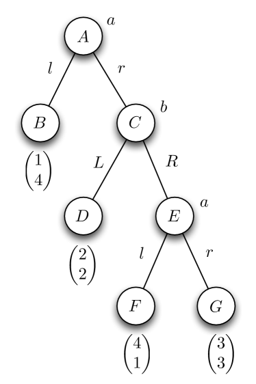
Figure 1.1: A simple extensive form game.

This model represents a situation where two players, $a$ and $b$, take turns, with $a$ starting at the top node $A$. If $a$ plays $l$ (‘left’) in this node, the game ends in node $B$ and the payoff for $a$ is $1$ and that for $b$ is $4$. If $a$, however, plays $r$ in $A$, the game proceeds to node $C$, where it is $b$’s turn. Player $b$ has a choice between playing $L$ and $R$ (note that we use upper case to distinguish $b$’s moves from $a$’s moves). The game continues until a terminal node is reached. We assume that both players are rational; that is, each prefers a higher outcome for themselves over a lower one. What will $a$ play in the start node $A$?

One way to determine what will happen in this game is to use backward. Consider node $E$. If that node is reached, given that $a$ is rational (denoted ${\mathit{r}at}_{a}$), $a$ will play $l$ here, since she prefers the outcome $4$ over $3$ (which she would get by playing $r$). Now consider node $C$. Since $b$ knows that $a$ is rational, he knows that his payoff when playing $R$ at $C$ is 1. Since $b$ is rational, and playing $L$ in $C$ gives him $2$, he will play $L$. The only thing needed to conclude this is $({\mathit{r}at}_{b}\land K_{b}{\mathit{r}at}_{a})$. Finally, consider node $A$. Player $a$ can reason as we just did, so $a$ knows that she has a choice between the payoff of $2$ she would obtain by playing $r$ and the payoff of $1$ she would obtain by playing $l$. Since $a$ is rational, she plays $r$ at $A$. Summarising, the condition that justifies $a$ playing $r$ at $A$ and $b$ playing $L$ at $B$ is

$${\mathit{r}at}_{a}\land K_{a}{\mathit{r}at_{b}}\land K_{a}K_{b}{\mathit{r}at}_{a}\land{\mathit{r}at}_{b}\land K_{b}{\mathit{r}at}_{a}$$

This analysis predicts that the game will end in node $D$. Although this analysis used only ‘depth-two’ knowledge ($a$ knows that $b$ knows), to perform a similar analysis for longer variants of this game requires deeper and deeper knowledge of rationality. In fact, in many epistemic analyses in game theory, common knowledge of rationality is assumed. The contribution of epistemic logic to game theory is discussed in more detail in Chapter 9.

1.2.1 Language

Most if not all systems presented in this book extend propositional logic. The language of propositional logic assumes a set $\mathsf{At}$ of primitive (or atomic) propositions, typically denoted $p,q,\dots$, possibly with subscripts. They typically refer to statements that are considered basic; that is, they lack logical structure, like ‘it is raining’, or ‘the window is closed’. Classical logic then uses Boolean operators, such as $\neg$ (‘not’), $\land$ (‘and’), $\lor$, (‘or’), $\rightarrow$ (‘implies’), and $\leftrightarrow$ (‘if and only if’), to build more complex formulas. Since all those operators can be defined in terms of $\land$ and $\neg$ (see Definition 1.2), the formal definition of the language often uses only these two connectives. Formulas are denoted with Greek letters: $\varphi,\psi,\alpha,\dots$. So, for instance, while $(p\land q)$ is the conjunction of two primitive propositions, the formula $(\varphi\land\psi)$ is a conjunction of two arbitrary formulas, each of which may have further structure.

When reasoning about knowledge and belief, we need to be able to refer to the subject, that is, the agent whose knowledge or belief we are talking about. To do this, we assume a finite set $\mathsf{Ag}$ of agents. Agents are typically denoted $a,b,\dots,i,j,\dots$, or, in specific examples, $\mathit{Alice},\mathit{Bob},\dots$. To reason about knowledge, we add operators $K_{a}$ to the language of classical logic, where $K_{a}\varphi$ denotes ‘agent $a$ knows (or believes) $\varphi$’. We typically let the context determine whether $K_{a}$ represents knowledge or belief. If it is necessary to reason knowledge and belief simultaneously, we use operators $K_{a}$ for knowledge and $B_{a}$ for belief. Logics for reasoning about knowledge are sometimes called epistemic logics, while logics for reasoning about belief are called doxastic logics, from the Greek words for knowledge and belief. The operators $K_{a}$ and $B_{a}$ are examples of modal operators. We sometimes use $\Box$ or $\Box_{a}$ to denote a generic modal operator, when we want to discuss general properties of modal operators.

Definition 1.1 (An Assemblage of Modal Languages).

Let $\mathsf{At}$ be a set of primitive propositions, $\mathsf{Op}$ a set of modal operators, and $\mathsf{Ag}$ a set of agent symbols. Then we define the language $\mathsf{L}(\mathsf{At},\mathsf{Op},\mathsf{Ag})$ by the following BNF:

$$\varphi:=p\ \mid\ \neg\varphi\ \mid\ (\varphi\land\varphi)\ \mid\ \Box\varphi,$$

where $p\in\mathsf{At}$ and $\Box\in\mathsf{Op}$. $\dashv$

Typically, the set $\mathsf{Op}$ depends on $\mathsf{Ag}$. For instance, the language for multi-agent epistemic logic is $\mathsf{L}(\mathsf{At},\mathsf{Op},\mathsf{Ag})$, with $\mathsf{Op}=\{K_{a}\mid a\in\mathsf{Ag}\}$, that is, we have a knowledge operator for every agent. To study interactions between knowledge and belief, we would have $\mathsf{Op}=\{K_{a},B_{a}\mid a\in\mathsf{Ag}\}$. The language of propositional logic, which does not involve modal operators, is denoted $\mathsf{L}(\mathsf{At})$; propositional formulas are, by definition, formulas in $\mathsf{L}(\mathsf{At})$.

Definition 1.2 (Abbreviations in the Language).

As usual, parentheses are omitted if that does not lead to ambiguity. The following abbreviations are also standard (in the last one, $A\subseteq\mathsf{Ag}$).

$$\begin{array}[]{l|l|l}\text{\it description/name}&\text{\it definiendum}&\text{\it definiens}\\ \hline\cr\textit{false}&\bot&p\wedge\neg p\\ \textit{true}&\top&\neg\bot\\ \text{disjunction}&\varphi\vee\psi&\neg(\neg\varphi\wedge\neg\psi)\\ \text{implication}&\varphi\rightarrow\psi&\neg\varphi\vee\psi\\ \text{dual of $K$}&M_{a}\varphi\text{ or }\hat{K}_{a}\varphi&\neg K_{a}\neg\varphi\\ \text{everyone in $A$ knows}&E_{A}\varphi&\bigwedge_{a\in A}K_{a}\varphi\\ \end{array}$$

Note that $M_{a}\varphi$, which say ‘agent $a$ does not know $\neg\varphi$’, can also be read ‘agent $a$ considers $\varphi$ possible’. $\dashv$

Let $\Box$ be a modal operator, either one in $\mathsf{Op}$ or one defined as an abbreviation. We define the $n$th iterated application of $\Box$, written $\Box^{n}$, as follows:

$$\Box^{0}\varphi=\varphi\mbox{ and }\Box^{n+1}\varphi=\Box\Box^{n}\varphi.$$

We are typically interested in iterating the $E_{A}$ operator, so that we can talk about ‘everyone in $A$ knows’, ‘everyone in $A$ knows that everyone in $A$ knows’, and so on.

Finally, we define two measures on formulas.

Definition 1.3 (Length and modal depth).

The length $\mid\!\varphi\!\mid$ and the modal depth $d(\varphi)$ of a formula $\varphi$ are both defined inductively as follows:

$$\begin{array}[]{lclclcl}\mid\!p\!\mid&=&1&\mbox{and}&d(p)&=&0\\ \mid\!\neg\varphi\!\mid&=&\mid\!\varphi\!\mid+1&\mbox{and}&d(\neg\varphi)&=&d(\varphi)\\ \mid\!(\varphi\land\psi)\!\mid&=&\mid\!\varphi\!\mid+\mid\!\psi\!\mid+1&\mbox{and}&d(\varphi\land\psi)&=&max\{d(\varphi),d(\psi)\}\\ \mid\!\Box_{a}\varphi\!\mid&=&\mid\!\varphi\!\mid+1&\mbox{and}&d(\Box\varphi)&=&1+d(\varphi).\end{array}$$

In the last clause, $\Box_{a}$ is a modal operator corresponding to a single agent. Sometimes, if $A\subseteq\mathsf{Ag}$ is a group of agents and $\Box_{A}$ is a group operator (like $E_{A}$, $D_{A}$ or $C_{A}$), $\mid\!\Box_{A}\varphi\!\mid$ depends not only on $\varphi$, but also on the cardinality of $A$. $\dashv$

So, $\mid\!\Box_{a}(q\land\Box_{b}p)\!\mid=5$ and $d(\Box_{a}(q\land\Box_{b}p))=2$. Likewise, $\mid\!\Box_{a}q\land\Box_{b}p\!\mid=5$ while $d(\Box_{a}q\land\Box_{b}p)=1$.

1.2.2 Semantics

We now define a way to systematically determine the truth value of a formula. In propositional logic, whether $p$ is true or not ‘depends on the situation’. The relevant situations are formalised using valuations, where a valuation

$$V:\mathsf{At}\rightarrow\{\mathit{true},\mathit{false}\}$$

determines the truth of primitive propositions. A valuation can be extended so as to determine the truth of all formulas, using a straightforward inductive definition: $\varphi\land\psi$ is true given $V$ iff each of $\varphi$ and $\psi$ is true given $V$, and $\neg\varphi$ is true given $V$ iff $\varphi$ is false given $V$. The truth conditions of disjunctions, implications, and bi-implications follow directly from these two clauses and Definition 1.2. To model knowledge and belief, we use ideas that go back to Hintikka. We think of an agent $a$ as considering possible a number of different situations that are consistent with the information that the agent has. Agent $a$ is said to know (or believe) $\varphi$, if $\varphi$ is true in all the situations that $a$ considers possible. Thus, rather than using a single situation to give meaning to modal formulas, we use a set of such situations; moreover, in each situation, we consider, for each agent, what other situations he or she considers possible. The following example demonstrates how this is done.

Example 1.1.

Bob is invited for a job interview with Alice. They have agreed that it will take place in a coffeehouse downtown at noon, but the traffic is quite unpredictable, so it is not guaranteed that either Alice or Bob will arrive on time. However, the coffeehouse is only a 15-minute walk from the bus stop where Alice plans to go, and a 10-minute walk from the metro station where Bob plans to go. So, 10 minutes before the interview, both Alice and Bob will know whether they themselves will arrive on time. Alice and Bob have never met before. A Kripke model describing this situation is given in Figure 1.2.

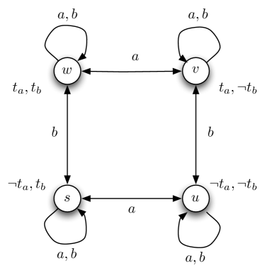
Figure 1.2: The Kripke model for Example 1.1.

Suppose that at 11:50, both Alice and Bob have just arrived at their respective stations. Taking $t_{a}$ and $t_{b}$ to represent that Alice (resp., Bob) arrive on time, this is a situation (denoted $w$ in Figure 1.2) where both $t_{a}$ and $t_{b}$ are true. Alice knows that $t_{a}$ is true (so in $w$ we have $K_{a}t_{a}$), but she does not know whether $t_{b}$ is true; in particular, Alice considers possible the situation denoted $v$ in Figure 1.2, where $t_{a}\land\neg t_{b}$ holds. Similarly, in $w$, Bob considers it possible that the actual situation is $s$, where Alice is running late but Bob will make it on time, so that $\neg t_{a}\land t_{b}$ holds. Of course, in $s$, Alice knows that she is late; that is, $K_{a}\neg t_{a}$ holds. Since the only situations that Bob considers possible at world $w$ are $w$ and $s$, he knows that he will be on time ($K_{b}t_{b}$), and knows that Alice knows whether or not she is on time ($K_{b}(K_{a}t_{a}\lor K_{a}\neg t_{a})$). Note that the latter fact follows since $K_{a}t_{a}$ holds in world $w$ and $K_{a}\neg t_{a}$ holds in world $s$, so $K_{a}t_{a}\lor K_{a}\neg t_{a}$ holds in both worlds that Bob considers possible. $\dashv$

This, in a nutshell, explains what the models for epistemic and doxastic look like: they contain a number of situations, typically called states or (possible) worlds, and binary relations on states for each agent, typically called accessibility relations. A pair $(v,w)$ is in the relation for agent $a$ if, in world $v$, agent $a$ considers state $w$ possible. Finally, in every state, we need to specify which primitive propositions are true.

Definition 1.4 (Kripke frame, Kripke model).

Given a set $\mathsf{At}$ of primitive propositions and a set $\mathsf{Ag}$ of agents, a Kripke model is a structure $M=\langle S,R^{\mathsf{Ag}},V^{\mathsf{At}})$, where

• $S\neq\emptyset$ is a set of states, sometimes called the domain of $M$, and denoted ${\mathcal{D}}(M)$;

• $R^{\mathsf{Ag}}$ is a function, yielding an accessibility relation $R_{a}\subseteq S\times S$ for each agent $a\in\mathsf{Ag}$;

• $V^{\mathsf{At}}:S\rightarrow(\mathsf{At}\rightarrow\{\mathit{true},\mathit{false}\})$ is a function that, for all $p\in\mathsf{At}$ and $s\in S$, determines what the truth value $V^{\mathsf{At}}(s)(p)$ of $p$ is in state $s$ (so $V^{\mathsf{At}}(s)$ is a propositional valuation for each $s\in S$).

We often suppress explicit reference to the sets $\mathsf{At}$ and $\mathsf{Ag}$, and write $M=\langle S,R,V\rangle$, without upper indices. Further, we sometimes write $sR_{a}t$ or $R_{a}st$ rather than $(s,t)\in R_{a}$, and use $R_{a}(s)$ or $R_{a}s$ to denote the set $\{t\in S\mid R_{a}st\}$. Finally, we sometimes abuse terminology and refer to $V$ as a valuation as well.

The class of all Kripke models is denoted $\mathcal{K}$. We use $\mathcal{K}_{m}$ to denote the class of Kripke models where $\mid\!\mathsf{Ag}\!\mid=m$. A Kripke frame $F=\langle S,R\rangle$ focuses on the graph underlying a model, without regard for the valuation. $\dashv$

More generally, given a modal logic with a set $\mathsf{Op}$ of modal operators, the corresponding Kripke model has the form $M=\langle S,R^{\mathsf{Op}},V^{\mathsf{At}}\rangle$, where there is a binary relation $R_{\Box}$ for every operator $\Box\in\mathsf{Op}$. $\mathsf{Op}$ may, for example, consist of a knowledge operator for each agent in some set $\mathsf{Ag}$ and a belief operator for each agent in $\mathsf{Ag}$.

Given Example 1.1 and Definition 1.4, it should now be clear how the truth of a formula is determined given a model $M$ and a state $s$. A pair $(M,s)$ is called a pointed model; we sometimes drop the parentheses and write $M,s$.

Definition 1.5 (Truth in a Kripke Model).

Given a model $M=\langle S,R^{\mathsf{Ag}},V^{\mathsf{At}}\rangle$, we define what it means for a formula $\varphi$ to be true in $(M,s)$, written $M,s\models\varphi$, inductively as follows:

$$\begin{array}[]{lll}M,s\models p&\mbox{iff}&V(s)(p)=\mathit{true}{\mbox{ for }p\in\mathsf{At}}\\ M,s\models\varphi\land\psi&\mbox{iff}&M,s\models\varphi\mbox{ and }M,s\models\psi\\ M,s\models\neg\varphi&\mbox{iff}&\mbox{not }M,s\models\varphi\ \mbox{ (often written $M,s\not\models\varphi$)}\\ M,s\models K_{a}\varphi&\mbox{iff}&M,t\models\varphi\mbox{ for all }t\mbox{ such that }R_{a}st.\end{array}$$

More generally, if $M=\langle S,R^{\mathsf{Op}},V^{\mathsf{At}}\rangle$, then for all $\Box\in\mathsf{Op}$:

$$M,s\models\Box\varphi\mbox{ iff }(M,t)\models\varphi\mbox{ for all }t\mbox{ such that }R_{\Box}st.$$

Recall that $M_{a}$ is the dual of $K_{a}$; it easily follows from the definitions that

$$M,s\models M_{a}\varphi\mbox{ iff there exists some $t$ such that }R_{a}st\mbox{ and }M,t\models\varphi.$$

We write $M\models\varphi$ if $M,s\models\varphi$ for all $s\in S$. $\dashv$

Example 1.2.

Consider the model of Figure 1.2. Note that $K_{a}p\lor K_{a}\neg p$ represents the fact that agent $a$ knows whether $p$ is true. Likewise, $M_{a}p\land M_{a}\neg p$ is equivalent to $\neg K_{a}\neg p\land\neg K_{a}p$: agent $a$ is ignorant about $p$. We have the following (in the final items we write $E_{ab}$ instead of $E_{\{a,b\}}$):

1. $(M,s)\models t_{b}$: truth of a primitive proposition in $s$.

2. $M,s\models(\neg t_{a}\land K_{a}\neg t_{a}\land\neg K_{b}\neg t_{a})\land(t_{b}\land\neg K_{a}t_{b}\land K_{b}t_{b})$: at $s$, $a$ knows that $t_{a}$ is false, but $b$ does not; similarly, $b$ knows that $t_{b}$ is true, but $a$ does not.

3. $M\models K_{a}(K_{b}t_{b}\lor K_{b}\neg t_{b})\land K_{b}(K_{a}t_{a}\lor K_{a}\neg t_{a})$: in all states of $M$, agent $a$ knows that $b$ knows whether $t_{b}$ is true, and $b$ knows that $a$ knows whether $t_{a}$ is true.

4. $M\models K_{a}(M_{b}t_{b}\land M_{b}\neg t_{b})\land K_{b}(M_{a}t_{a}\land M_{a}\neg t_{a})$ in all states of $M$, agent $a$ knows that $b$ does not know whether $t_{a}$ is true, and $b$ knows that $a$ does not know whether $t_{b}$ is true.

5. $M\models E_{ab}((K_{a}t_{a}\lor K_{a}\neg t_{a})\land(M_{a}t_{b}\land M_{a}\neg t_{b}))$: in all states, everyone knows that $a$ knows whether $t_{a}$ is true, but $a$ does not know whether $t_{b}$ is true.

6. $M\models E_{ab}E_{ab}((K_{a}t_{a}\lor K_{a}\neg t_{a})\land(M_{a}t_{b}\land M_{a}\neg t_{b}))$: in all states, everyone knows what we stated in the previous item.

This shows that the model $M$ of Figure 1.2 is not just a model for a situation where $a$ knows $t_{a}$ but not $t_{b}$ and agent $b$ knows $t_{b}$ but not $t_{a}$; it represents much more information. $\dashv$

As the following example shows, in order to model certain situations, it may be necessary that some propositional valuations occur in more than one state in the model.

Example 1.3.

Recall the scenario of the interview between Alice and Bob, as presented in Example 1.1. Suppose that we now add the information that in fact Alice will arrive on time, but Bob is not going to be on time. Although Bob does not know Alice, he knows that his friend Carol is an old friend of Alice. Bob calls Carol, leaving a message on her machine to ask her to inform Alice about Bob’s late arrival as soon as she is able to do so. Unfortunately for Bob, Carol does not get his message on time. This situation can be represented in state $M,v$ of the model of Figure 1.3.

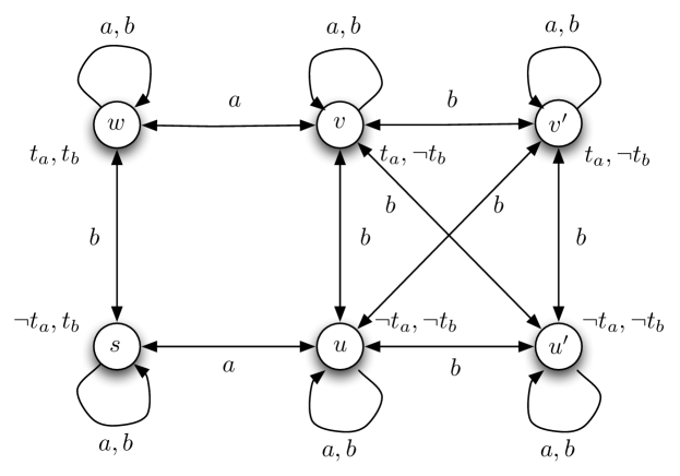
Figure 1.3: The Kripke model for Example 1.3.

Note that in $(M,v)$, we have $\neg K_{a}\neg t_{b}$ (Alice does not know that Bob is late), but also $M_{b}(K_{a}\neg t_{b})$ (Bob considers it possible that Alice knows that Bob is late). So, although the propositional valuations in $v$ and $v^{\prime}$ are the same, those two states represent different situations: in $v$ agent $a$ is uncertain whether $\neg t_{b}$ holds, while in $v^{\prime}$ she knows $\neg t_{b}$. Also, in $M,v$, Bob considers it possible that both of them will be late, and that Alice knows this: this is because $R_{b}vu^{\prime}$ holds in the model, and $M,u^{\prime}\models K_{a}(\neg t_{a}\land\neg t_{b})$. $\dashv$

We often impose restrictions on the accessibility relation. For example, we may want to require that if, in world $v$, agent $a$ considers world $w$ possible, then in $w$, agent $a$ should consider $v$ possible. This requirement would make $R_{a}$ symmetric. Similarly, we might require that, in each world $w$, $a$ considers $w$ itself possible. This would make $R_{a}$ reflexive. More generally, we are interested in certain subclasses of models (typically characterized by properties of the accessibility relations).

Definition 1.6 (Classes of models, validity, satisfiability).

Let $\mathcal{X}$ be a class of models, that is, $\mathcal{X}\subseteq\mathcal{K}$. If $M\models\varphi$ for all models $M$ in $\mathcal{X}$, we say that $\varphi$ is valid in $\mathcal{X}$, and write $\mathcal{X}\models\varphi$. For example, for validity in the class of all Kripke models $\mathcal{K}$, we write $\mathcal{K}\models\varphi$. We write $\mathcal{X}\not\models\varphi$ when it is not the case that $\mathcal{X}\models\varphi$. So $\mathcal{X}\not\models\varphi$ holds if, for some model $M\in\mathcal{X}$ and some $s\in{\mathcal{D}}(M)$, we have $M,s\models\neg\varphi$. If there exists a model $M\in\mathcal{X}$ and a state $s\in{\mathcal{D}}({M})$ such that $M,s\models\varphi$, we say that $\varphi$ is satisfiable in $\mathcal{X}$. $\dashv$

We now define a number of classes of models in terms of properties of the relations $R_{a}$ in those models. Since they depend only on the accessibility relation, we could have defined them for the underlying frames; indeed, the properties are sometimes called frame properties.

Definition 1.7 (Frame properties).

Let $R$ be an accessibility relation on a domain of states $S$.

1. $R$ is serial if for all $s$ there is a $t$ such that $Rst$. The class of serial Kripke models, that is, $\{M=\langle S,R,V\rangle\mid\mbox{ every }R_{a}\mbox{ is serial}\}$ is denoted $\mathcal{KD}$.

2. $R$ is reflexive if for all $s$, $Rss$. The class of reflexive Kripke models is denoted $\mathcal{KT}$.

3. $R$ is transitive if for all $s,t,u$, if $Rst$ and $Rtu$ then $Rsu$. The class of transitive Kripke models is denoted $\mathcal{K}4$.

4. $R$ is Euclidean if for all $s,t,$ and $u$, if $Rst$ and $Rsu$ then $Rtu$. The class of Euclidean Kripke models is denoted $\mathcal{K}5$

5. $R$ is symmetric if for all $s,t$, if $Rst$ then $Rts$. The class of symmetric Kripke models is denoted $\mathcal{KB}$

6. We can combine properties of relations:

   1. The class of reflexive transitive models is denoted $\mathcal{S}4$.

   2. The class of transitive Euclidean models is denoted $\mathcal{K}45$.

   3. The class of serial transitive Euclidean models is denoted $\mathcal{KD}45$.

   4. $R$ is an equivalence relation if $R$ is reflexive, symmetric, and transitive. It not hard to show that $R$ is an equivalence relation if $R$ is reflexive and Euclidean. The class of models where the relations are equivalence relations is denoted $\mathcal{S}5$.

As we did for $\mathcal{K}_{m}$, we sometimes use the subscript $m$ to denote the number of agents, so $\mathcal{S}5_{m}$, for instance, is the class of Kripke models with $\mid\!\mathsf{Ag}\!\mid=m$. $\dashv$

Of special interest in this book is the class $\mathcal{S}5$. In this case, the accessibility relations are equivalence classes. This makes sense if we think of $R_{a}st$ holding if $s$ and $t$ are indistinguishable by agent $a$ based on the information that $a$ has received. $\mathcal{S}5$ has typically been used to model knowledge. In an $\mathcal{S}5$ model, write $s\sim_{a}t$ rather than $R_{a}st$, to emphasize the fact that $R_{a}$ is an equivalence relation. When it is clear that $M\in\mathcal{S}5$, when drawing the model, we omit reflexive arrows, and since the relations are symmetric, we connect states by a line, rather than using two-way arrows. Finally, we leave out lines that can be deduced to exist using transitivity. We call this the S5 representation of a Kripke model. Figure 1.4 shows the S5 representation of the Kripke model of Figure 1.3.

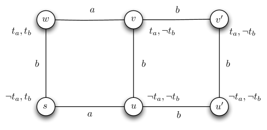
Figure 1.4: The S5 representation of the Kripke model in Figure 1.3.

When we restrict the classes of models considered, we get some interesting additional valid formulas.

Theorem 1.1 (Valid Formulas).

Parts (c)–(i) below are valid formulas, where $\alpha$ is a substitution instance of a propositional tautology (see below), $\varphi$ and $\psi$ are arbitrary formulas, and $\mathcal{X}$ is one of the classes of models defined in Definition 1.7; parts (a), (b), and (j) show that we can infer some valid formulas from others.

1. If $\mathcal{X}\models\varphi\rightarrow\psi$ and $\mathcal{X}\models\varphi$, then $\mathcal{X}\models\psi$.

2. If $\mathcal{X}\models\varphi$ then $\mathcal{X}\models K\varphi$.

3. $\mathcal{X}\models\alpha$.

4. $\mathcal{X}\models K(\varphi\rightarrow\psi)\rightarrow(K\varphi\rightarrow\psi)$.

5. $\mathcal{KD}\models K\varphi\rightarrow M\varphi$.

6. $\mathcal{T}\models K\varphi\rightarrow\varphi$.

7. $\mathcal{K}4\models K\varphi\rightarrow KK\varphi$.

8. $\mathcal{K}5\models\neg K\varphi\rightarrow K\neg K\varphi$.

9. $\mathcal{KB}\models\varphi\rightarrow KM\varphi$.

10. If $\mathcal{X}\subseteq\mathcal{Y}$ then $\mathcal{Y}\models\varphi$ implies that $\mathcal{X}\models\varphi$.

$\dashv$

Since $\mathcal{S}5$ is the smallest of the classes of models considered in Definition 1.7, it easily follows that all the formulas and inference rules above are valid in $\mathcal{S}5$. To the extent that we view $\mathcal{S}5$ as the class of models appropriate for reasoning about knowledge, Theorem 1.1 can be viewed as describing properties of knowledge. As we shall see, many of these properties apply to the standard interpretation of belief as well.

Parts (a) and (c) emphasise that we represent knowledge in a logical framework: modus ponens is valid as a reasoning rule, and we take all propositional tautologies for granted. In part (c), $\alpha$ is a substitution instance of a propositional tautology. For example, since $p\lor\neg p$ and $p\rightarrow(q\rightarrow p)$ are propositional tautologies, $\alpha$ could be $Kp\lor\neg Kp$ or $K(p\lor q)\rightarrow(Kr\rightarrow K(p\lor q))$. That is, we can substitute an arbitrary formula (uniformly) for a primitive proposition in a propositional tautology. Part (b) says that agents know all valid formulas, and part (d) says that an agent is able to apply modus ponens to his own knowledge. Part (e) is equivalent to $K\varphi\rightarrow\neg K\neg\varphi$; an agent cannot at the same time know a proposition and its negation. Part (f) is even stronger: it says that what an agent knows must be true. Parts (g) and (h) represent what has been called positive and negative introspection, respectively: an agent knows what he knows and what he does not know. Part (i) can be shown to follow from the other valid formulas; it says that if something is true, the agent knows that he considers it possible.

Notions of Group Knowledge

So far, all properties that we have encountered are properties of an individual agent’s knowledge. such as $E_{A}$, defined above. In this section we introduce two other notions of group knowledge, common knowledge $C_{A}$ and distributed knowledge $D_{A}$, and investigate their properties.

Example 1.4 (Everyone knows and distributed knowledge).

Alice and Betty each has a daughter; their children can each either be at the playground (denoted $p_{a}$ and $p_{b}$, respectively) or at the library ($\neg p_{a}$, and $\neg p_{b}$, respectively). Each child has been carefully instructed that, if she ends up being on the playground without the other child, she should call her mother to inform her. Consider the situation described by the model $M$ in Figure 1.5.

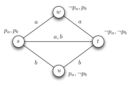
Figure 1.5: The (S5 representation of the) model for Example 1.4.

We have

$$M\models((\neg p_{a}\land p_{b})\leftrightarrow K_{a}(\neg p_{a}\land p_{b}))\land((p_{a}\land\neg p_{b})\leftrightarrow K_{b}(p_{a}\land\neg p_{b})).$$

This models the agreement each mother made with her daughter. Now consider the situation at state $s$. We have $M,s\models K_{a}\neg(p_{a}\land\neg p_{b})$, that is, Alice knows that it is not the case that her daughter is alone at the playground (otherwise her daughter would have informed her). What does each agent know at $s$? If we consider only propositional facts, it is easy to see that Alice knows $p_{a}\rightarrow p_{b}$ and Betty knows $p_{b}\rightarrow p_{a}$. What does everyone know at $s$? The following sequence of equivalences is immediate from the definitions:

$$\begin{array}[]{ll}&M,s\models E_{\{a,b\}}\varphi\\ \mbox{iff}&M,s\models K_{a}\varphi\land K_{b}\varphi\\ \mbox{iff}&\forall x(R_{a}sx\Rightarrow M,x\models\varphi)\ \mbox{ and }\ \forall y(R_{b}sy\Rightarrow M,y\models\varphi)\\ \mbox{iff}&\forall x\in\{s,w,t\}\,(M,x\models\varphi)\mbox{ and }\forall y\in\{s,u,t\}\,(M,y\models\varphi)\\ \mbox{iff}&M\models\varphi.\end{array}$$

Thus, in this model, what is known by everyone are just the formulas valid in the model. Of course, this is not true in general.

Now suppose that Alice and Betty an opportunity to talk to each other. Would they gain any new knowledge? They would indeed. Since $M,s\models K_{a}(p_{a}\rightarrow p_{b})\land K_{b}(p_{b}\rightarrow p_{a})$, they would come to know that $p_{a}\leftrightarrow p_{b}$ holds; that is, they would learn that their children are at least together, which is certainly not valid in the model. The knowledge that would emerge if the agents in a group $A$ were allowed to communicate is called distributed knowledge in $A$, and denoted by the operator $D_{A}$. In our example, we have $M,s\models D_{\{a,b\}}(p_{a}\leftrightarrow p_{b})$, although $M,s\models\neg K_{a}(p_{a}\leftrightarrow p_{b})\land\neg K_{b}(p_{a}\leftrightarrow p_{b})$. In other words, distributed knowledge is generally stronger than any individual’s knowledge, and we therefore cannot define $D_{A}\varphi$ as $\bigvee_{i\in A}K_{i}\varphi$, the dual of general knowledge that we may have expected; that would be weaker than any individual agent’s knowledge. In terms of the model, what would happen if Alice and Betty could communicate is that Alice could tell Betty that he should not consider state $u$ possible, while Betty could tell Alice that she should not consider state $w$ possible. So, after communication, the only states considered possible by both agents at state $s$ are $s$ and $t$. This argument suggests that we should interpret $D_{A}$ as the necessity operator ($\Box$-type modal operator) of the relation $\bigcap_{a\in A}R_{a}$. By way of contrast, it follows easily from the definitions that $E_{A}$ can be interpreted as the necessity operator of the relation $\bigcup_{a\in A}R_{a}$. $\dashv$

The following example illustrates common knowledge.

Example 1.5 (Common knowledge).

This time we have two agents: a sender ($s$) and a receiver ($r$). If a message is sent, it is delivered either immediately or with a one-second delay. The sender sends a message at time $t_{0}$. The receiver does not know that the sender was planning to send the message. What is each agent’s state of knowledge regarding the message?

To reason about this, let $s_{z}$ (for $z\in\mathbb{Z}$) denote that the message was sent at time $t_{0}+z$, and, likewise, let $d_{z}$ denote that the message was delivered at time $t=z$. Note that we allow $z$ to be negative. To see why, consider the world $w_{0,0}$ where the message arrives immediately (at time $t_{0}$). (In general, in the subscript $(i,j)$ of a world $w_{i,j}$, $i$ denotes the time that the message was sent, and $j$ denotes the time it was received.) In world $w_{0,0}$, the receiver considers it possible that the message was sent at time $t_{0}-1$. That is, the receiver considers possible the world $w_{-1,0}$ where the message was sent at $t_{0}-1$ and took one second to arrive. In world $w_{-1,0}$, the sender considers possible the world $w_{-1,-1}$ where the message was sent at time $t_{0}-1$ and arrived immediately. And in world $w_{-1,-1}$, the receiver considers possible a world $w_{-2,-1}$ where the message as sent at time $t_{0}-2$. (In general, in world $w_{n,m}$, the message is sent at time $t_{0}+n$ and received at time $t_{0}+m$.) In addition, in world $w_{0,0}$, the sender considers possible world $w_{0,1}$, where the message is received at time $t_{0}+1$. The situation is described in the following model $M$.

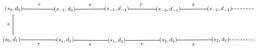
Figure 1.6: The (S5 representation of the) model for Example 1.5.

Writing $E$ for ‘the sender and receiver both know’, it easily follows that

$$M,w_{0,0}\models s_{0}\land d_{0}\land\neg E\neg s_{-1}\land\neg E\neg d_{1}\land\neg E^{3}\neg s_{-2}.$$

The notion of $\varphi$ being common knowledge among group $A$, denoted $C_{A}\varphi$, is meant to capture the idea that, for all $n$, $E^{n}\varphi$ is true. Thus, $\varphi$ is not common among $A$ if someone in $A$ considers it possible that someone in $A$ considers it possible that …someone in $A$ considers it possible that $\varphi$ is false. This is formalised below, but the reader should already be convinced that in our scenario, even if it is common knowledge among the agents that messages will have either no delay or a one-second delay, it is not common knowledge that the message was sent at or after time $t_{0}-m$ for any value of $m$! $\dashv$

Definition 1.8 (Semantics of three notions of group knowledge).

Let $A\subseteq\mathsf{Ag}$ be a group of agents. Let $R_{E_{A}}=\cup_{a\in A}R_{a}$. As we observed above,

$$(M,s)\models E_{A}\varphi\mbox{ iff for all $t$ such that }R_{E_{A}}st,\mbox{ we have }(M,t)\models\varphi.$$

Similarly, taking $R_{D_{A}}=\cap_{a\in A}R_{a}$, we have

$$(M,s)\models D_{A}\varphi\mbox{ iff for all $t$ such that }R_{D_{A}}st,\mbox{ we have }(M,t)\models\varphi.$$

Finally, recall that the transitive closure of a relation $R$ is the smallest relation $R^{+}$ such that $R\subseteq R^{+}$, and such that, for all $x,y,$ and $z$, if $R^{+}xy$ and $R^{+}yz$ then $R^{+}xz$. We define $R_{C_{A}}$ as $R_{E_{A}}^{+}=(\bigcup_{a\in A}R_{a})^{+}$. Note that, in Figure 1.6, every pair of states is in the relation $R_{C_{\{r,s\}}}^{+}$. In general, we have $R_{C_{A}}st$ iff there is some path $s=s_{0},s_{1},\dots,s_{n}=t$ from $s$ to $t$ such that $n\geq 1$ and, for all $i<n$, there is some agent $a\in A$ for which $R_{a}s_{i}s_{i+1}$. Define

$$(M,s)\models C_{A}\varphi\mbox{ iff for all $t$ such that }R_{C_{A}}st,(M,t)\models\varphi.$$

$\dashv$

It is almost immediate from the definitions that, for $a\in A$, we have

$$\mathcal{K}\models(C_{A}\varphi\rightarrow E_{A}\varphi)\land(E_{A}\varphi\rightarrow K_{a}\varphi)\land(K_{a}\varphi\rightarrow D_{A}\varphi).$$ (1.1)

Moreover, for $\mathcal{T}$ (and hence also for $\mathcal{S}4$ and $\mathcal{S}5$), we have

$$\mathcal{T}\models D_{a}\varphi\rightarrow\varphi.$$

The relative strengths shown in (1.1) are strict in the sense that none of the converse implications are valid (assuming that $A\neq\{a\}$).

We conclude this section by defining some languages that are used later in this chapter. Fixing $\mathsf{At}$ and $\mathsf{Ag}$, we write $\mathsf{L}_{X}$ for the language $\mathsf{L}(\mathsf{At},\mathsf{Op},\mathsf{Ag})$, where

$$\begin{array}[]{ll}X=K&\mbox{if }\mathsf{Op}=\{K_{a}\mid a\in\mathsf{Ag}\}\\ X=CK&\mbox{if }\mathsf{Op}=\{K_{a},C_{A}\mid a\in\mathsf{Ag},A\subseteq\mathsf{Ag}\}\\ X=DK&\mbox{if }\mathsf{Op}=\{K_{a},D_{A}\mid a\in\mathsf{Ag},A\subseteq\mathsf{Ag}\}\\ X=CDK&\mbox{if }\mathsf{Op}=\{K_{a},C_{A},D_{A}\mid a\in\mathsf{Ag},A\subseteq\mathsf{Ag}\}\\ X=EK&\mbox{if }\mathsf{Op}=\{K_{a},E_{A}\mid a\in\mathsf{Ag},A\subseteq\mathsf{Ag}\}.\\ \end{array}$$

Bisimulation

It may well be that two models $(M,s)$ and $(M^{\prime},s^{\prime})$ ‘appear different’, but still satisfy the same formulas. For example, consider the models $(M,s)$, $(M^{\prime},s^{\prime})$, and $(N,s_{1})$ in Figure 1.7. As we now show, they satisfy the same formulas. We actually prove something even stronger. We show that all of $(M,s)$, $(M,t)$, $(M^{\prime},s^{\prime})$, $(N,s_{1})$, $(M,s_{2})$, and $(N,s_{3})$ satisfy the same formulas, as do all of $(M,u)$, $(M,w)$, $(M^{\prime},w^{\prime})$, $(N,w_{1})$, and $(N,w_{2})$. For the purposes of the proof, call the models in the first group green, and the models in the second group red. We now show, by induction on the structure of formulas, that all green models satisfy the same formulas, as do all red models. For primitive propositions, this is immediate. And if two models of the same colour agree on two formulas, they also agree on their negations and their conjunctions. The other formulas we need to consider are knowledge formulas. Informally, the argument is this. Every agent considers, in every pointed model, both green and red models possible. So his knowledge in each pointed model is the same. We now formalise this reasoning.

Definition 1.9 (Bisimulation).

Given models $M=(S,R,V)$ and $M^{\prime}=(S^{\prime},R^{\prime},V^{\prime})$, a non-empty relation $\mathfrak{R}\subseteq S\times S^{\prime}$ is a bisimulation between $M$ and $M^{\prime}$ iff for all $s\in S$ and $s^{\prime}\in S^{\prime}$ with $(s,s^{\prime})\in\mathfrak{R}$:

• $V(s)(p)=V^{\prime}(s^{\prime})(p)$ for all $p\in\mathsf{At}$;

• for all $a\in\mathsf{Ag}$ and all $t\in S$, if $R_{a}st$, then there is a $t^{\prime}\in S^{\prime}$ such that $R^{\prime}_{a}s^{\prime}t^{\prime}$ and $(t,t^{\prime})\in\mathfrak{R}$;

• for all $a\in\mathsf{Ag}$ and all $t^{\prime}\in S^{\prime}$, if $R^{\prime}_{a}s^{\prime}t^{\prime}$, then there is a $t\in S$ such that $R_{a}st$ and $(t,t^{\prime})\in\mathfrak{R}$.

We write $(M,s){\raisebox{1.29167pt}[0.0pt][0.0pt]{$\medspace\underline{\!\leftrightarrow\!}\medspace$}}(M^{\prime},s^{\prime})$ iff there is a bisimulation between $M$ and $M^{\prime}$ linking $s$ and $s^{\prime}$. If so, we call $(M,s)$ and $(M^{\prime},s^{\prime})$ bisimilar. $\dashv$

Figure 1.7 illustrates some bisimilar models.

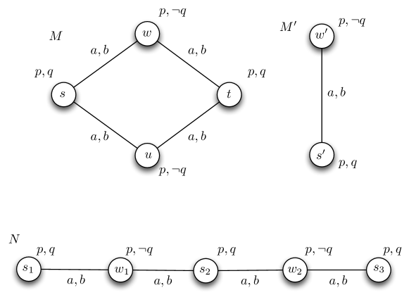
Figure 1.7: Bisimilar models.

In terms of the models of Figure 1.7, we have $M,s{\raisebox{1.29167pt}[0.0pt][0.0pt]{$\medspace\underline{\!\leftrightarrow\!}\medspace$}}M^{\prime},s^{\prime}$, $M,s{\raisebox{1.29167pt}[0.0pt][0.0pt]{$\medspace\underline{\!\leftrightarrow\!}\medspace$}}N,s_{1}$, etc. We are interested in bisimilarity because, as the following theorem shows, bisimilar models satisfy the same formulas involving the operators $K_{a}$ and $C_{A}$.

Theorem 1.2 (Preservation under bisimulation).

Suppose that $(M,s){\raisebox{1.29167pt}[0.0pt][0.0pt]{$\medspace\underline{\!\leftrightarrow\!}\medspace$}}(M^{\prime},s^{\prime})$. Then, for all formulas $\varphi\in\mathsf{L}_{CK}$, we have

$$M,s\models\varphi\Leftrightarrow M^{\prime},s^{\prime}\models\varphi.$$

$\dashv$

The proof of the theorem proceeds by induction on the structure of formulas, much as in our example. We leave the details to the reader.

Note that Theorem 1.2 does not claim that distributed knowledge is preserved under bisimulation, and indeed, it is not, i.e., Theorem 1.2 does not hold for a language with $D_{A}$ as an operator. Figure 1.8 provides a witness for this. We leave it to the reader to check that although $(M,s){\raisebox{1.29167pt}[0.0pt][0.0pt]{$\medspace\underline{\!\leftrightarrow\!}\medspace$}}(N,s_{1})$ for the two pointed models of Figure 1.8, we nevertheless have $(M,s)\models\neg D_{\{a,b\}}p$ and $(N,s_{1})\models D_{\{a,b\}}p$.

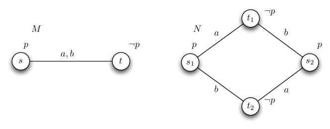
Figure 1.8: Two bisimilar models that do not preserve distributed knowledge.

We can, however, generalise the notion of bisimulation to that of a group bisimulation and ‘recover’ the preservation theorem, as follows. If $A\subseteq\mathsf{Ag}$, $s$ and $t$ are states, then we write $R_{A}st$ if $A=\{a\mid R_{a}st\}$. That is, $R_{A}st$ holds if the set of agents $a$ for which $s$ and $t$ are $a$-connected is exactly $A$. $(M,s)$ and $(M^{\prime},s^{\prime})$ are group bisimilar, written $(M,s){\raisebox{1.29167pt}[0.0pt][0.0pt]{$\medspace\underline{\!\leftrightarrow\!}\medspace$}}_{\mathit{g}roup}(M^{\prime},s^{\prime})$, if the conditions of Definition 1.9 are met when every occurrence of an individual agent $a$ is replaced by the group $A$. Obviously, being group bisimilar implies being bisimilar. Note that the models $(M,s)$ and $(N,s_{1})$ of Figure 1.8 are bisimilar, but not group bisimilar. The proof of Theorem 1.3 is analogous to that of Theorem 1.2.

Theorem 1.3 (Preservation under bisimulation).

Suppose that $(M,s){\raisebox{1.29167pt}[0.0pt][0.0pt]{$\medspace\underline{\!\leftrightarrow\!}\medspace$}}_{\mathit{g}roup}(M^{\prime},s^{\prime})$. Then, for all formulas $\varphi\in\mathsf{L}_{CDK}$, we have

$$M,s\models\varphi\Leftrightarrow M^{\prime},s^{\prime}\models\varphi.$$

$\dashv$

1.2.3 Expressivity and Succinctness

If a number of formal languages can be used to model similar phenomena, a natural question to ask is which language is ‘best’. Of course, the answer depends on how ‘best’ is measured. In the next section, we compare various languages in terms of the computational complexity of some reasoning problems. Here, we consider the notions of expressivity (what can be expressed in the language?) and succinctness (how economically can one say it?).

Expressivity

To give an example of expressivity and the tools that are used to study it, we start by showing that finiteness of models cannot be expressed in epistemic logic, even if the language includes operators for common knowledge and distributed knowledge.

Theorem 1.4.

There is no formula $\varphi\in\mathsf{L}_{CDK}$ such that, for all $\mathcal{S}5$-models $M=\langle S,R,V\rangle$,

$$M\models\varphi\mbox{ iff }S\mbox{ is finite}$$

$\dashv$

Proof.

Consider the two models $M$ and $M^{\prime}$ of Figure 1.9.

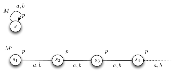
Figure 1.9: A finite and an infinite model where the same formulas are valid.

Obviously, $M$ is finite and $M^{\prime}$ is not. Nevertheless, the two models are easily seen to be group bisimilar, so they cannot be distinguished by epistemic formulas. More precisely, for all formulas $\varphi\in\mathsf{L}_{CDK}$, we have $M,s\models\varphi$ iff $M^{\prime},s_{1}\models\varphi$ iff $M^{\prime},s_{2}\models\varphi$ iff $M^{\prime},s_{n}\models\varphi$ for some $n\in\mathbb{N}$, and hence $M\models\varphi$ iff $M^{\prime}\models\varphi$.

It follows immediately from Theorem 1.4 that finiteness cannot be expressed in the language $\mathsf{L}_{CDK}$ in a class ${\mathcal{X}}$ of models containing ${\mathcal{S}}5$.

We next prove some results that let us compare the expressivity of two different languages. We first need some definitions.

Definition 1.10.

Given a class ${\mathcal{X}}$ of models, formulas $\varphi_{1}$ and $\varphi_{2}$ are equivalent on ${\mathcal{X}}$, written $\varphi_{1}\equiv_{\mathcal{X}}\varphi_{2}$, if, for all $(M,s)\in\mathcal{X}$, we have that $M,s\models\varphi_{1}$ iff $M,s\models\varphi_{2}$. Language $\mathsf{L}_{2}$ is at least as expressive as $\mathsf{L}_{1}$ on ${\mathcal{X}}$, written $\mathsf{L}_{1}\sqsubseteq_{\mathcal{X}}\mathsf{L}_{2}$ if, for every formula $\varphi_{1}\in\mathsf{L}_{1}$, there is a formula $\varphi_{2}\in\mathsf{L}_{2}$ such that $\varphi_{1}\equiv_{\mathcal{X}}\varphi_{2}$. $\mathsf{L}_{1}$ and $\mathsf{L}_{2}$ are equally expressive on ${\mathcal{X}}$ if $\mathsf{L}_{1}\sqsubseteq_{\mathcal{X}}\mathsf{L}_{2}$ and $\mathsf{L}_{2}\sqsubseteq_{\mathcal{X}}\mathsf{L}_{1}$. If $\mathsf{L}_{1}\sqsubseteq_{\mathcal{X}}\mathsf{L}_{2}$ but $\mathsf{L}_{2}\not\sqsubseteq_{\mathcal{X}}\mathsf{L}_{1}$, then $\mathsf{L}_{2}$ is more expressive than $\mathsf{L}_{1}$ on ${\mathcal{X}}$, written $\mathsf{L}_{1}\sqsubset_{\mathcal{X}}\mathsf{L}_{2}$. $\dashv$

Note that if ${\mathcal{Y}}\subseteq{\mathcal{X}}$, then $\mathsf{L}_{1}\sqsubseteq_{\mathcal{X}}\mathsf{L}_{2}$ implies $\mathsf{L}_{1}\sqsubseteq_{\mathcal{Y}}\mathsf{L}_{2}$, while $\mathsf{L}_{1}\not\sqsubseteq_{\mathcal{Y}}\mathsf{L}_{2}$ implies $\mathsf{L}_{1}\not\sqsubseteq_{\mathcal{X}}\mathsf{L}_{2}$. Thus, the strongest results that we can show for the classes of models of interest to us are $\mathsf{L}_{1}\sqsubseteq_{\mathcal{K}}\mathsf{L}_{2}$ and $\mathsf{L}_{1}\not\sqsubseteq_{\mathcal{S}5}\mathsf{L}_{2}$

With these definitions in hand, we can now make precise that common knowledge ‘really adds’ something to epistemic logic.

Theorem 1.5.

$\mathsf{L}_{K}\sqsubseteq_{\mathcal{K}}\mathsf{L}_{CK}$ and $\mathsf{L}_{K}\not\sqsubseteq_{\mathcal{S}5}\mathsf{L}_{CK}$. $\dashv$

Proof.

Since $\mathsf{L}_{K}\subseteq\mathsf{L}_{CK}$, it is obvious that $\mathsf{L}_{K}\sqsubseteq_{\mathcal{K}}\mathsf{L}_{CK}$. To show that $\mathsf{L}_{CK}\not\sqsubseteq_{\mathcal{S}5}\mathsf{L}_{K}$, consider the sets of pointed models ${\mathcal{M}}=\{(M_{n},s_{1})\mid n\in\mathbb{N}\}$ and ${\mathcal{N}}=\{(N_{n},t_{1})\mid n\in\mathbb{N}\}$ shown in Figure 1.10. The two models $M_{n}$ and $N_{n}$ differ only in $(M_{n},s_{n+1})$ (where $p$ is false) and $(N_{n},t_{n+1})$ (where $p$ is true). In particular, the first $n-1$ states of $(M_{n},s_{1})$ and $(N_{n},t_{1})$ are the same. As a consequence, it is easy to show that,

$$\mbox{for all }n\in\mathbb{N}\mbox{ and }\varphi\in\mathsf{L}_{K}\mbox{ with }d(\varphi)<n,\ (M_{n},s_{1})\models\varphi\mbox{ iff }(N_{n},t_{1})\models\varphi.$$ (1.2)

Clearly ${\mathcal{M}}\models C_{\{a,b\}}\neg p$ while ${\mathcal{N}}\models\neg C_{\{a,b\}}\neg p$. If there were a formula $\varphi\in\mathsf{L}_{K}$ equivalent to $C_{\{a,b\}}\neg p$, then we would have ${\mathcal{M}}\models\varphi$ while ${\mathcal{N}}\models\neg\varphi$. Let $d=d(\varphi)$, and consider the pointed models $(M_{d+1},s_{1})$ and $(N_{d+1},t_{1})$. Since the first is a member of ${\mathcal{M}}$ and the second of ${\mathcal{N}}$, the pointed models disagree on $C_{\{a,b\}}\neg p$; however, by (1.2), they agree on $\varphi$. This is obviously a contradiction, therefore a formula $\varphi\in\mathsf{L}$ that is equivalent to $C_{\{a,b\}}\neg p$ does not exist.

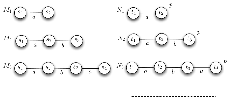
Figure 1.10: Models $M_{n}$ and $N_{n}$. The atom $p$ is only true in the pointed models $(N_{n},s_{n+1})$.

The next result shows, roughly speaking, that distributed knowledge is not expressible using knowledge and common knowledge, and that common knowledge is not expressible using knowledge and distributed knowledge.

Theorem 1.6.

1. $\mathsf{L}_{K}\sqsubseteq_{\mathcal{K}}\mathsf{L}_{DK}$ and $\mathsf{L}_{K}\not\sqsubseteq_{\mathcal{S}5}\mathsf{L}_{DK}$;

2. $\mathsf{L}_{CK}\not\sqsubseteq_{\mathcal{S}5}\mathsf{L}_{DK}$;

3. $\mathsf{L}_{DK}\not\sqsubseteq_{\mathcal{S}5}\mathsf{L}_{CK}$;

4. $\mathsf{L}_{CK}\sqsubseteq_{\mathcal{K}}\mathsf{L}_{CDK}$ and $\mathsf{L}_{CDK}\not\sqsubseteq_{\mathcal{S}5}\mathsf{L}_{CK}$;

5. $\mathsf{L}_{DK}\sqsubseteq_{\mathcal{K}}\mathsf{L}_{CDK}$ and $\mathsf{L}_{CDK}\not\sqsubseteq_{\mathcal{S}5}\mathsf{L}_{DK}$.

$\dashv$

Proof.

For part (a), $\sqsubseteq_{\mathcal{K}}$ holds trivially. We use the models in Figure 1.8 to show that $\mathsf{L}_{DK}\not\sqsubseteq_{\mathcal{S}5}\mathsf{L}_{K}$. Since $(M,s){\raisebox{1.29167pt}[0.0pt][0.0pt]{$\medspace\underline{\!\leftrightarrow\!}\medspace$}}(N,s_{1})$, the models verify the same $\mathsf{L}$-formulas. However, $\mathsf{L}_{DK}$ discriminates them: we have $(M,s)\models\neg D_{\{a,b\}}p$, while $(N,s_{1})\models D_{\{a,b\}}p$. Since $(M,s)$ and $(N,s_{1})$ also verify the same $\mathsf{L}_{CK}$-formulas, part (3) also follows.

For part (b), observe that (1.2) is also true for all formulas $\varphi\in\mathsf{L}_{DK}$, so the formula $C_{\{a,b\}}\neg p\in\mathsf{L}_{CK}$ is not equivalent to a formula in $\mathsf{L}_{DK}$.

Part (c) is proved using exactly the same models and argument as part (a).

For part (d), $\sqsubseteq$ is obvious. To show that $\mathsf{L}_{CDK}\not\sqsubseteq_{{\mathcal{S}}5}\mathsf{L}_{DK}$, we can use the models and argument of part (b). Similarly, for part (e), $\sqsubseteq$ is obvious. To show that $\mathsf{L}_{CDK}\not\sqsubseteq_{{\mathcal{S}}5}\mathsf{L}_{DK}$, we can use the models and argument of part (a).

We conclude this discussion with a remark about distributed knowledge. We informally described distributed knowledge in a group as the knowledge that would obtain were the agents in that group able to communicate. However, Figure 1.8 shows that this intuition is not quite right. First, observe that both $a$ and $b$ know the same formulas in $(M,s)$ and $(N,s_{1})$; they even know the same formulas in $(M,s)$ and $(N,s_{1})$. That is, for all $\varphi\in\mathsf{L}_{K}$, we have

$$(M,s)\models K_{a}\varphi\mbox{ iff }(M,s)\models K_{b}\varphi\mbox{ iff }(N,s_{1})\models K_{a}\varphi\mbox{ iff }(N,s_{1})\models K_{b}\varphi$$

But if both agents possess the same knowledge in $(N,s_{1})$, how can communication help them in any way, that is, how can it be that there is distributed knowledge (of $p$) that no individual agent has? Similarly, if $a$ has the same knowledge in $(M,s)$ in $(N,s_{1})$, and so does $b$, why would communication in one model ($N$) lead them to know $p$, while in the other, it does not? Semantically, one could argue that in $s_{1}$ agent $a$ could ‘tell’ agent $b$ that $t_{2}$ ‘is not possible’, and $b$ could ‘tell’ $a$ that $t_{1}$ ‘is not possible’. But how would verify the same formulas? This observation has led some researchers to require that distributed knowledge be interpreted in what are called bisimulation contracted models (see the notes at the end of the chapter for references). Roughly, a model is bisimulation contracted if it does not contain two points that are bisimilar. Model $M$ of Figure 1.8 is bisimulation contracted, model $N$ is not.

Succinctness

Now suppose that two languages $\mathsf{L}_{1}$ and $\mathsf{L}_{2}$ are equally expressive on ${\mathcal{X}}$, and also that their computational complexity of the reasoning problems for them is equally good, or equally bad. Could we still prefer one language over the other? Representational succinctness may provide an answer here: it may be the case that the description of some properties is much shorter in one language than in the other.

But what does ‘much shorter’ mean? The fact that there is a formula $\mathsf{L}_{1}$ whose length is 100 characters less than the shortest equivalent formula in $\mathsf{L}_{2}$ (with respect to some class $\mathcal{X}$ of models) does not by itself make $\mathsf{L}_{1}$ much more succinct that $\mathsf{L}_{2}$.

We want to capture the idea that $\mathsf{L}_{1}$ is exponentially more succinct than $\mathsf{L}_{2}$. We cannot do this by looking at just one formula. Rather, we need a sequence of formulas $\alpha_{1},\alpha_{2},\alpha_{3},\ldots$ in $\mathsf{L}_{1}$, where the gap in size between $\alpha_{n}$ and the shortest formula equivalent to $\alpha_{n}$ in $\mathsf{L}_{2}$ grows exponentially in $n$. This is formalised in the next definition.

Definition 1.11 (Exponentially more succinct).

Given a class ${\mathcal{X}}$ of models, $\mathsf{L}_{1}$ is exponentially more succinct than $\mathsf{L}_{2}$ on ${\mathcal{X}}$ if the following conditions hold:

1. for every formula $\beta\in\mathsf{L}_{2}$, there is a formula $\alpha\in\mathsf{L}_{1}$ such that $\alpha\equiv_{\mathcal{X}}\beta$ and $\mid\!\alpha\!\mid\leq\mid\!\beta\!\mid$.

2. there exist $k_{1},k_{2}>0$, a sequence $\alpha_{1},\alpha_{2},\ldots$ of formulas in $\mathsf{L}_{1}$, and a sequence $\beta_{1},\beta_{2},\ldots$ of formulas in $\mathsf{L}_{2}$ such that, for all $n$, we have:

   • $\mid\!\alpha_{n}\!\mid\leq k_{1}n$;

   • $\mid\!\beta_{n}\!\mid\ \geq 2^{k_{2}n}$;

   • $\beta_{n}$ is the shortest formula in $\mathsf{L}_{2}$ that is equivalent to $\alpha_{n}$ on ${\mathcal{X}}$.

$\dashv$

In words, $\mathsf{L}_{1}$ is exponentially more succinct than $\mathsf{L}_{2}$ if, for every formula $\beta\in\mathsf{L}_{2}$, there is a formula in $\mathsf{L}_{1}$ that is equivalent and no longer than $\beta$, but there is a sequence $\alpha_{1},\alpha_{2},\ldots$ of formulas in $\mathsf{L}_{1}$ whose length increases at most linearly, but there is no sequence $\beta_{1},\beta_{2},\ldots$ of formulas in $\mathsf{L}_{2}$ such that $\beta_{n}$ is the equivalent to $\alpha_{n}$ and the length of the formulas in the latter sequence is increasing better than exponentially.

We give one example of succinctness results here. Consider the language $\mathsf{L}_{EK}$. Of course, $E_{A}$ can be defined using the modal operators $K_{i}$ for $i\in A$. But, as we now show, having the modal operators $E_{A}$ in the language makes the language exponentially more succinct.

Theorem 1.7.

The language $\mathsf{L}_{EK}$ is exponentially more succinct than $\mathsf{L}_{K}$ on $\mathcal{X}$, for all $X$ between $\mathcal{K}$ and $\mathcal{S}5$. $\dashv$

Proof.

Clearly, for every formula $\alpha$ in $\mathsf{(}L)_{K}$, there is an equivalent formula in $\mathsf{L}_{EK}$ that is no longer than $\alpha$, namely, $\alpha$ itself. Now consider the following two sequences of formulas:

$$\alpha_{n}=\neg E^{n}_{\{a,b\}}\neg p$$

and

$$\beta_{1}=\neg(K_{a}\neg p\land K_{b}\neg p),\mbox{ and }\beta_{n}=\neg(K_{a}\neg\beta_{n-1}\land K_{b}\neg\beta_{n-1}).$$

If we take $\mid\!E_{A}\varphi\!\mid=\mid\!A\!\mid+\mid\!\varphi\!\mid$, then it is easy to see that $\mid\!\alpha_{n}\!\mid=2n+3$, so $\mid\!\alpha_{n}\!\mid$ is increasing linearly in $n$. On the other hand, since $\mid\!\beta_{n}\!\mid>2\mid\!\beta_{n-1}\!\mid$, we have $\mid\!\beta\!\mid\geq 2^{n}$. It is also immediate from the definition of $E_{\{a,b\}}$ that $\beta_{n}$ is equivalent to $\alpha_{n}$ for all classes $\mathcal{X}$ between $\mathcal{K}$ and $\mathcal{S}5$. To complete the proof, we must show that there is no formula shorter than $\beta_{n}$ in $\cal{L}_{K}$ that is equivalent to $\alpha_{n}$. This argument is beyond the scope of this book; see the notes for references.

1.2.4 Reasoning problems

Given the machinery developed so far, we can state some basic reasoning problems in semantic terms. They concern satisfiability and model checking. Most of those problems are typically considered with a specific class of models and a specific language in mind. So let $\mathcal{X}$ be some class of models, and let $\mathsf{L}$ be a language.

Decidability Problems

A decidability problem checks some input for some property, and returns ‘yes’ or ‘no’.

Definition 1.12 (Satisfiability).

The satisfiability problem for $\mathcal{X}$ is the following reasoning problem.

Problem: satisfiability in $\mathcal{X}$, denoted sat_X. Input: a formula $\varphi\in\mathsf{L}$. Question: does there exist a model $M\in\mathcal{X}$ and a state $s\in{\mathcal{D}}(M)$ such that $M,s\models\varphi$? Output: ‘yes’ or ‘no’.
$\dashv$

Obviously, there may well be formulas that are satisfiable in some Kripke model (or generally, in a class $\mathcal{Y}$), but not in $\mathcal{S}5$ models. Satisfiability in $\mathcal{X}$ is closely related to the problem of validity in $\mathcal{X}$, due to the following equivalence: $\varphi$ is valid in $\mathcal{X}$ iff $\neg\varphi$ is not satisfiable in $\mathcal{X}$.

Problem: validity in $\mathcal{X}$, denoted val_X. Input: a formula $\varphi\in\mathsf{L}$. Question: is it the case that $\mathcal{X}\models\varphi$? Output: ‘yes’ or ‘no’.  

The next decision problem is computationally and conceptually simpler than the previous two, since rather than quantifying over a set of models, a specific model is given as input (together with a formula).

Definition 1.13 (Model checking).

The model checking problem for $\mathcal{X}$ is the following reasoning problem:

Problem: Model checking in $\mathcal{X}$, denoted modcheck_X. Input: a formula $\varphi\in\mathsf{L}$ and a pointed model $(M,s)$ with $M\in\mathcal{X}$ and $s\in{\mathcal{D}}(M)$. Question: is it the case that $M,s\models\varphi$? Output:: ‘yes’ or ‘no’.
$\dashv$

The field of computational complexity is concerned with the question of how much of a resource is needed to solve a specific problem. The resources of most interest are computation time and space. Computational complexity then asks questions of the following form: if my input were to increase in size, how much more space and/or time would be needed to compute the answer? Phrasing the question this way already assumes that the problem at hand can be solved in finite time using an algorithm, that is, that the problem is decidable. Fortunately, this is the case for the problems of interest to us.

Proposition 1.1 (Decidability of sat and modcheck).

If $\mathcal{X}$ is one of the model classes defined in Definition 1.7, $(M,s)\in\mathcal{X}$, and $\varphi$ is a formula in one of the languages defined in Definition 1.1, then both sat${}_{\mathcal{X}}(\varphi)$ and modcheck${}_{\mathcal{X}}((M,s),\varphi)$ are decidable. $\dashv$

In order to say anything sensible about the additional resources that an algorithm needs to compute the answer when the input increases in size, we need to define a notion of size for inputs, which in our case are formulas and models. Formulas are by definition finite objects, but models can in principle be infinite (see, for instance, Figure 1.6). The following fact is the key to proving Fact 1.1. For a class of models $\mathcal{X}$, let $\mathcal{F}in(\mathcal{X})\subseteq\mathcal{X}$ be the set of models in $\mathcal{X}$ that are finite.

Proposition 1.2 (Finite model property).

For all classes of models in Definition 1.7 and languages $\mathsf{L}$ in Definition 1.1, we have, for all $\varphi\in\mathsf{L}$,

$$\mathcal{X}\models\varphi\mbox{ iff }\mathcal{F}in(\mathcal{X})\models\varphi.$$

$\dashv$

Fact 1.2 does not say that the models in $\mathcal{X}$ and the finite models in $\mathcal{X}$ are the same in any meaningful sense; rather, it says that we do not gain valid formulas if we restrict ourselves to finite models. It implies that a formula is satisfiable in a model in $\mathcal{X}$ iff it is satisfiable in a finite model in $\mathcal{X}$. It follows that in the languages we have considered so far, ‘having a finite domain’ is not expressible (for if there were a formula $\varphi$ that were true only of models with finite domains, then $\varphi$ would be a counterexample to Fact 1.2).

Definition 1.14 (Size of Models).

For a finite model $M=\langle S,^{\mathsf{Ag}},V^{\mathsf{At}}\rangle$, the size of $M$, denoted $\|M\|$, is the sum of the number of states ($\mid\!S\!\mid$, for which we also write $\mid\!M\!\mid$) and the number of pairs in the accessibility relation ($\mid\!R_{a}\!\mid$) for each agent $a\in\mathsf{Ag}$. $\dashv$

We can now strengthen Fact 1.2 as follows.

Proposition 1.3.

For all classes of models in Definition 1.7 and languages $\mathsf{L}$ in Definition 1.1, we have, for all $\varphi\in\mathsf{L}$, $\varphi$ is satisfiable in $\mathcal{X}$ iff there is a model $M\in\mathcal{X}$ such that $\mid\!{\mathcal{D}}(M)\!\mid\leq 2^{\mid\!\,\varphi\,\!\mid}$ and $\varphi$ is satisfiable in $M$. $\dashv$

The idea behind the proof of Proposition 1.3 is that states that ‘agree’ on all subformulas of $\varphi$ can be ‘identified’. Since there are only $\mid\!\varphi\!\mid$ subformulas of $\varphi$, and $2^{\mid\!\,\varphi\,\!\mid}$ truth assignments to these formulas, the result follows. Of course, work needs to done to verify this intuition, and to show that an appropriate model can be constructed in the right class $\mathcal{X}$.

To reason about the complexity of a computation performed by an algorithm, we distinguish various complexity classes. If a deterministic algorithm can solve a problem in time polynomial in the size of the input, the problem is said to be in P. An example of a problem in P is to decide, given two finite Kripke models $M_{1}$ and $M_{2}$, whether there exists a bisimulation between them. Model checking for the basic multi-modal language is also in P; see Proposition 1.4.

In a nondeterministic computation, an algorithm is allowed to ‘guess’ which of a finite number of steps to take next. A nondeterministic algorithm for a decision problem says ‘yes’ or accepts the input if the algorithm says ‘yes’ to an appropriate sequence of guesses. So a nondeterministic algorithm can be seen as generating different branches at each computation step, and the answer of the nondeterministic algorithm is ‘yes’ iff one of the branches results in a ‘yes’ answer.

The class NP is the class of problems that are solvable by a nondeterministic algorithm in polynomial time. Satisfiability of propositional logic is an example of a problem in NP: an algorithm for satisfiability first guesses an appropriate truth assignment to the primitive propositions, and then verifies that the formula is in fact true under this truth assignment.

A problem that is at least as hard as any problem in NP is called NP-hard. An NP-hard problem has the property that any problem in NP can be reduced to it using a polynomial-time reduction. A problem is NP-complete if it is both in NP and NP-hard; satisfiability for propositional logic is well known to be NP-complete. For an arbitrary complexity class C, notions of C-hardness and C-completeness can be similarly defined.

Many other complexity classes have been defined. We mention a few of them here. An algorithm that runs in space polynomial in the size of the input it is in PSPACE. Clearly if an algorithm needs only polynomial time then it is in polynomial space; that is P $\subseteq$ PSPACE. In fact, we also have NP $\subseteq$ PSPACE. If an algorithm is in NP, we can run it in polynomial space by systematically trying all the possible guesses, erasing the space used after each guess, until we eventually find one that is the ‘right’ guess. EXPTIME consists of all algorithms that run in time exponential in the size of the input; NEXPTIME is its nondeterministic analogue. We have P $\subseteq$ NP $\subseteq$ PSPACE $\subseteq$ EXPTIME $\subseteq$ NEXPTIME. One of the most important open problems in computer science is the question whether P = NP. The conjecture is that the two classes are different, but this has not yet been proved; it is possible that a polynomial-time algorithm will be found for an NP-hard problem. What is known is that P $\neq$ EXPTIME and NP $\neq$ NEXPTIME.

The complement $\bar{P}$ of a problem $P$ is the problem in which all the ‘yes’ and ‘no’ answers are reversed. Given a complexity class C, the class co-C is the set of problems for which the complement is in C. For every deterministic class C, we have co-C = C. For nondeterministic classes, a class and its complement are, in general, believed to be incomparable. Consider, for example, the satisfiability problem for propositional logic, which, as we noted above, is NP-complete. Since a formula $\varphi$ is valid if and only if $\neg\varphi$ is not satisfiable, it easily follows that the validity problem for propositional logic is co-NP-complete. The class of NP-complete and co-NP-complete problems are believed to be distinct.

We start our summary of complexity results for decision problems in modal logic with model checking.

Proposition 1.4.

Model checking formulas in $\mathsf{L}(\mathsf{At},\mathsf{Op},\mathsf{Ag})$, with $\mathsf{Op}=\{K_{a}\mid a\in\mathsf{Ag}\}$, in finite models is in P. $\dashv$

Proof.

We now describe an algorithm that, given a model $M=\langle S,R^{\mathsf{Ag}},$ $V^{\mathsf{At}}\rangle$ and a formula $\varphi\in\mathsf{L}$, determines in time polynomial in $\mid\!\varphi\!\mid$ and $\|M\|$ whether $M,s\models\varphi$. Given $\varphi$, order the subformulas $\varphi_{1},\dots\varphi_{m}$ of $\varphi$ in such a way that, if $\varphi_{i}$ is a subformula of $\varphi_{j}$, then $i<j$. Note that $m\leq{\mid\!\varphi\!\mid}$. We claim that

(*) for every $k\leq m$, we can label each state $s$ in $M$ with either $\varphi_{j}$ (if $\varphi_{j}$ if true at $s$) or $\neg\varphi_{j}$ (otherwise), for every $j\leq k$, in $k\|M\|$ steps.

We prove (*) by induction on $m$. If $k=1$, $\varphi_{m}$ must be a primitive proposition, and obviously we need only ${\mid\!M\!\mid}\leq{\|M\|}$ steps to label all states as required. Now suppose (*) holds for some $k<m$, and consider the case $k+1$. If $\varphi_{k+1}$ is a primitive proposition, we reason as before. If $\varphi_{k+1}$ is a negation, then it must be $\neg\varphi_{j}$ for some $j\leq k$. Using our assumption, we know that the collection of formulas $\varphi_{1},\dots,\varphi_{k}$ can be labeled in $M$ in $k\|M\|$ steps. Obviously, if we include $\varphi_{k+1}=\neg\varphi_{j}$ in the collection of formulas, we can do the labelling in $k$ more steps: just use the opposite label for $\varphi_{k+1}$ as used for $\varphi_{i}$. So the collection $\varphi_{1},\dots,\varphi_{k+1}$ can be labelled in $M$ in at $(k+1)\|M\|$ steps, are required. Similarly, if $\varphi_{k+1}=\varphi_{i}\land\varphi_{j}$, with $i,j\leq k$, a labelling for the collection $\varphi_{1},\dots,\varphi_{k+1}$ needs only $(k+1)\|M\|$ steps: for the last formula, in each state $s$ of $M$, the labelling can be completed using the labellings for $\varphi_{i}$ and $\varphi_{j}$. Finally, suppose $\varphi_{k+1}$ is of the form $K_{a}\varphi_{j}$ with $j\leq k$. In this case, we label a state $s$ with $K_{a}\varphi_{j}$ iff each state $t$ with $R_{a}st$ is labelled $\varphi_{j}$. Assuming the labels $\varphi_{j}$ and $\neg\varphi_{j}$ are already in place, this can be done in $\mid\!R_{a}(s)\!\mid\leq\|M\|$ steps.

Proposition 1.4 should be interpreted with care. While having a polynomial-time procedure seems attractive, we are talking about computation time polynomial in the size of the input. To model an interesting scenario or system often requires ‘big models’. Even for one agent and $n$ primitive propositions, a model might consist of $2^{n}$ states. Moreover, the procedure does not check properties of the model either, for instance whether it belongs to a given class $\mathcal{X}$.

We now formulate results for satisfiability checking. The results depend on two parameters: the class of models considered (we focus on $\mathcal{K},\mathcal{T},\mathcal{S}4,\mathcal{KD}45$ and $\mathcal{S}5$) and the language. Let $\mathsf{Ag}_{=1}$ consist of only one agent, let $\mathsf{Ag}_{\geq 1}\neq\emptyset$ be an arbitrary set of agents, and let $\mathsf{Ag}_{\geq 2}$ be a set of at least two agents. Finally, let $\mathsf{Op}=\{K_{a}\mid a\in\mathsf{Ag}\}$.

Theorem 1.8 (Satisfiability).

The complexity of the satisfiability problem is

1. NP-complete if $\mathcal{X}\in\{\mathcal{KD}45,\mathcal{S}5\}$ and $\mathsf{L}=\mathsf{L}(\mathsf{At},\mathsf{Op},\mathsf{Ag}_{=1})$;

2. PSPACE-complete if

   1. $\mathcal{X}\in\{\mathcal{K},\mathcal{T},\mathcal{S}4\}$ and $\mathsf{L}=\mathsf{L}(\mathsf{At},\mathsf{Op},\mathsf{Ag}_{\geq 1})$, or

   2. $\mathcal{X}\in\{\mathcal{KD}45,\mathcal{S}5\}$ and $\mathsf{L}=\mathsf{L}(\mathsf{At},\mathsf{Op},\mathsf{Ag}_{\geq 2})$;

3. EXPTIME-complete if

   1. $\mathcal{X}\in\{\mathcal{K},\mathcal{T}$ and $\mathsf{L}=\mathsf{L}(\mathsf{At},\mathsf{Op}\cup\{C\},\mathsf{Ag}_{\geq 1})$, or

   2. $\mathcal{X}\in\{\mathcal{S}4,\mathcal{KD}45,\mathcal{S}5\}$ and $\mathsf{L}=\mathsf{L}(\mathsf{At},\mathsf{Op}\cup\{C\},\mathsf{Ag}_{\geq 2})$.

$\dashv$

From the results in Theorem 1.8, it follows that the satisfiability problem for logics of knowledge and belief for one agent, $\mathcal{S}5$ and $\mathcal{KD}45$, is exactly as hard as the satisfiability problem for propositional logic. If we do not allow for common knowledge, satisfiability for the general case is PSPACE-complete, and with common knowledge it is EXPTIME-complete. (Of course, common knowledge does not add anything for the case of one agent.)

For validity, the consequences of Theorem 1.8 are as follows. We remarked earlier that if satisfiability (in $\mathcal{X}$) is in some class C, then validity is in co-C. Hence, checking validity for the cases in item 1 is co-NP-complete. Since co-PSPACE = PSPACE, the validity problem for the cases in item 2 is PSPACE-complete, and, finally, since co-EXPTIME = EXPTIME, the validity problem for the cases in item 3 is EXPTIME-complete. What these results on satisfiability and validity mean in practice? Historically, problems that were not in P were viewed as too hard to deal with in practice. However, recently, major advances have been made in finding algorithms that deal well with many NP-complete problems, although no generic approaches have been found for dealing with problems that are co-NP-complete, to say nothing of problems that are PSPACE-complete and beyond. Nevertheless, even for problems in these complexity classes, algorithms with humans in the loop seem to provide useful insights. So, while these complexity results suggest that it is unlikely that we will be able to find tools that do automated satisfiability or validity checking and are guaranteed to always give correct results for the logics that we focus on in this book, this should not be taken to say that we cannot write algorithms for satisfiability, validity, or model checking that are useful for the problems of practical interest. Indeed, there is much work focused on just that.

1.2.5 Axiomatisation

In the previous section, the formalisation of reasoning was defined around the notion of truth: $\mathcal{X}\models\varphi$ meant that $\varphi$ is true in all models in $\mathcal{X}$. In this section, we discuss a form of reasoning where a conclusion is inferred purely based on its syntactic form. Although there are several ways to do this, in epistemic logic, the most popular way to define deductive inference is by defining a Hilbert-style axiom system. Such systems provide a very simple notion of formal proofs. Some formulas are valid merely because they have a certain syntactic form. These are the axioms of the system. The rules of the system say that one can conclude that some formula is valid due to other formulas being valid. A formal proof or derivation is a list of formulas, where each formula is either an axiom of the system or can be obtained by applying an inference rule of the system to formulas that occur earlier in the list. A proof or derivation of $\varphi$ is a derivation whose last formula is $\varphi$.

Basic system

Our first definition of such a system will make the notion more concrete. We give our definitions for a language where the modal operators are $K_{a}$ for the agents in some set $\mathsf{Ag}$, although many of the ideas generalise to a setting with arbitrary modal operators.

Definition 1.15 (System $\mathbf{K}$).

Let $\mathsf{L}=\mathsf{L}(\mathsf{At},\mathsf{Op},\mathsf{Ag})$, with $\mathsf{Op}=\{K_{a}\mid a\in\mathsf{Ag}\}$. The axiom system $\mathbf{K}$ consists of the following axioms and rules of inference:

$\mathbf{1}$ All substitution instances of propositional tautologies. $\mathbf{K}$ $K_{a}(\varphi\rightarrow\psi)\rightarrow(K_{a}\varphi\rightarrow K_{a}\psi)$ for all $a\in\mathsf{Ag}$. $\mathbf{MP}$ From $\varphi$ and $\varphi\rightarrow\psi$ infer $\psi$. $\mathbf{Nec}$ From $\varphi$ infer $K_{a}\varphi$.

$\dashv$

Here, formulas in the axioms $\mathbf{1}$ and $\mathbf{K}$ have to be interpreted as axiom schemes: axiom $\mathbf{K}$ for instance denotes all formulas $\{K_{a}(\varphi\rightarrow\psi)\rightarrow(K_{a}\varphi\rightarrow K_{a}\psi)\mid\varphi,\psi\in\mathsf{L}\}$. The rule $\mathbf{MP}$ is also called modus ponens; $\mathbf{Nec}$ is called necessitation. Note that the notation for axiom $\mathbf{K}$ and the axiom system $\mathbf{K}$ are the same: the context should make clear which is intended.

To see how an axiom system is actually used, we need to define the notion of derivation.

Definition 1.16 (Derivation).

Given a logical language $\mathsf{L}$, let $\mathbf{X}$ be an axiom system with axioms $\mathbf{Ax_{1}},\dots,$ $\mathbf{Ax_{n}}$ and rules $\mathbf{Ru_{1}},\dots\mathbf{Ru_{k}}$. A derivation of $\varphi$ in X is a finite sequence $\varphi_{1},\dots,\varphi_{m}$ of formulas such that: (a) $\varphi_{m}=\varphi$, and (b) every $\varphi_{i}$ in the sequence is either an instance of an axiom or else the result of applying a rule to formulas in the sequence prior to $\varphi_{i}$. For the rules $\mathbf{MP}$ and $\mathbf{Nec}$, this means the following:

MP

$\varphi_{h}=\varphi_{j}\rightarrow\varphi_{i}$, for some $h,j<i$.

That is, both $\varphi_{j}$ and $\varphi_{j}\rightarrow\varphi_{i}$ occur in th sequence before $\varphi_{i}$.

Nec

$\varphi_{i}=K_{a}\varphi_{j}$, for some $j<i$;

If there is a derivation for $\varphi$ in $\mathbf{X}$ we write $\mathbf{X}\vdash\varphi$, or $\vdash_{\mathbf{X}}\varphi$, or, if the system X is clear from the context, we just write $\vdash\varphi$. We then also say that $\varphi$ is a theorem of $\mathbf{X}$, or that $\mathbf{X}$ proves $\varphi$. The sequence $\varphi_{1},\dots,\varphi_{m}$ is then also called a proof of $\varphi$ in $\mathbf{X}$. $\dashv$

Example 1.6 (Derivation in $\mathbf{K}$).

We first show that

$$\mathbf{K}\vdash K_{a}(\varphi\land\psi)\rightarrow(K_{a}\varphi\land K_{a}\psi).$$ (1.3)

We present the proof as a sequence of numbered steps (so that the formula $\varphi_{i}$ in the derivation is given number $i$). This allows us to justify each step in the proof by describing which axioms, rules of inference, and previous steps in the proof it follows from.

$\begin{array}[]{@{}l@{~}ll}1.\hfil~{}&(\varphi\land\psi)\rightarrow\varphi&\mathbf{1}\\ 2.\hfil~{}&K_{a}((\varphi\land\psi)\rightarrow\varphi)&\mathbf{Nec},1\\ 3.\hfil~{}&K_{a}((\varphi\land\psi)\rightarrow\varphi)\rightarrow(K_{a}(\varphi\land\psi)\rightarrow K_{a}\varphi)&\mathbf{K}\\ 4.\hfil~{}&K_{a}(\varphi\land\psi)\rightarrow K_{a}\varphi&\mathbf{MP},2,3\\ 5.\hfil~{}&(\varphi\land\psi)\rightarrow\psi&\mathbf{1}\\ 6.\hfil~{}&K_{a}((\varphi\land\psi)\rightarrow\psi)&\mathbf{Nec},5\\ 7.\hfil~{}&K_{a}((\varphi\land\psi)\rightarrow\psi)\rightarrow(K_{a}(\varphi\land\psi)\rightarrow K_{a}\psi)&\mathbf{K}\\ 8.\hfil~{}&K_{a}(\varphi\land\psi)\rightarrow K_{a}\psi&\mathbf{MP},6,7\\ 9.\hfil~{}&(K_{a}(\varphi\land\psi)\rightarrow K_{a}\varphi)\rightarrow\\ \hfil~{}&((K_{a}(\varphi\land\psi)\rightarrow K_{a}\psi)\rightarrow(K_{a}(\varphi\land\psi)\rightarrow(K_{a}\varphi\land K_{a}\psi)))&\mathbf{1}\\ 10.\hfil~{}&(K_{a}(\varphi\land\psi)\rightarrow K_{a}\psi)\rightarrow(K_{a}(\varphi\land\psi)\rightarrow(K_{a}\varphi\land K_{a}\psi))&\mathbf{MP},4,9\\ 11.\hfil~{}&K_{a}(\varphi\land\psi)\rightarrow(K_{a}\varphi\land K_{a}\psi)&\mathbf{MP},8,10\\ \end{array}$

Lines 1, 5, and 9 are instances of propositional tautologies (this can be checked using a truth table). Note that the tautology on line 9 is of the form $(\alpha\rightarrow\beta)\rightarrow((\alpha\rightarrow\gamma)\rightarrow(\alpha\rightarrow(\beta\land\gamma)))$. A proof like that above may look cumbersome, but it does show what can be done using only the axioms and rules of $\mathbf{K}$. It is convenient to give names to properties that are derived, and so build a library of theorems. We have, for instance that $\mathbf{K}\vdash\mathbf{KCD}$, where $\mathbf{KCD}$ (‘$K$-over-conjunction-distribution’) is

$$\mathbf{KCD}\ \ K_{a}(\alpha\land\beta)\rightarrow K_{a}\alpha\mbox{ and }K_{a}(\alpha\land\beta)\rightarrow K_{a}\beta.$$

The proof of this follows steps 1 - 4 and steps 5 - 8, respectively, of the proof above. We can also derive new rules; for example, the following rule: $\mathbf{CC}$ (‘combine conclusions’) is derivable in $\mathbf{K}$:

$$\mathbf{CC}\ \ \mbox{from }\alpha\rightarrow\beta\mbox{ and }\alpha\rightarrow\gamma\mbox{ infer }\alpha\rightarrow(\beta\land\gamma).$$

The proof is immediate from the tautology on line 9 above, to which we can, given the assumptions, apply modus ponens twice. We can give a more compact proof of $K_{a}(\varphi\land\psi)\rightarrow(K_{a}\varphi\land K_{a}\psi)$ using this library:

$$\begin{array}[]{lll}1.&K_{a}(\varphi\land\psi)\rightarrow K_{a}\varphi&\mathbf{KCD}\\ 2.&K_{a}(\varphi\land\psi)\rightarrow K_{a}\psi&\mathbf{KCD}\\ 3.&K_{a}(\varphi\land\psi)\rightarrow(K_{a}\varphi\land K_{a}\psi)&\mathbf{CC},1,2\end{array}$$

$\dashv$

For every class $\mathcal{X}$ of models introduced in the previous section, we want to have an inference system $\mathbf{X}$ such that derivability in $\mathbf{X}$ and validity in $\mathcal{X}$ coincide:

Definition 1.17 (Soundness and Completeness).

Let $\mathsf{L}$ be a language, let $\mathcal{X}$ be a class of models, and let $\mathbf{X}$ be an axiom system. The axiom system is said to be

1. sound for $\mathcal{X}$ and the language $\mathsf{L}$ if, for all formulas $\varphi\in\mathsf{L}$, $\mathbf{X}\vdash\varphi$ implies $\mathcal{X}\models\varphi$; and

2. complete for $\mathcal{X}$ and the language $\mathsf{L}$ if, for all formulas $\varphi\in\mathsf{L}$, $\mathcal{X}\models\varphi$ implies $\mathbf{X}\vdash\varphi$.

$\dashv$

We now provide axioms that characterize some of the subclasses of models that were introduced in Definition 1.7.

Definition 1.18 (More axiom systems).

Consider the following axioms, which apply for all agents $a\in\mathsf{Ag}$:

$\begin{array}[]{llr}\mathbf{T}.&K_{a}\varphi\rightarrow\varphi&\\ \mathbf{D}.&M_{a}\top&\\ \mathbf{B}.&\varphi\rightarrow K_{a}M_{a}\varphi\\ \mathbf{4}.&K_{a}\varphi\rightarrow K_{a}K_{a}\varphi\\ \mathbf{5}.&\neg K_{a}\varphi\rightarrow K_{a}\neg K_{a}\varphi\\ \end{array}$

A simple way to denote axiom systems is just to add the axioms that are included together with the name $\mathbf{K}$. Thus, $\mathbf{KD}$ is the axiom system that has all the axioms and rules of the system $\mathbf{K}$ ($\mathbf{1}$, $\mathbf{K}$, and rules $\mathbf{MP}$ and $\mathbf{Nec}$) together with $\mathbf{D}$. Similarly, $\mathbf{KD45}$ extends $\mathbf{K}$ by adding the axioms $\mathbf{D}$, $\mathbf{4}$ and $\mathbf{5}$. System $\mathbf{S4}$ is the more common way of denoting $\mathbf{KT4}$, while $\mathbf{S5}$ is the more common way of denoting $\mathbf{KT45}$. If it is necessary to make explicit that there are $m$ agents in $\mathsf{Ag}$, we write $\mathbf{K}_{m}$, $\mathbf{KD}_{m}$, and so on. $\dashv$

Using $\mathbf{S5}$ to model knowledge

The system $\mathbf{S5}$ is an extension of $\mathbf{K}$ with the so-called ‘properties of knowledge’. Likewise, $\mathbf{KD45}$ has been viewed as characterizing the ‘properties of belief’. The axiom $\mathbf{T}$ expresses that knowledge is veridical: whatever one knows, must be true. (It is sometimes called the truth axiom.) The other two axioms specify so-called introspective agents: $\mathbf{4}$ says that an agent knows what he knows (positive introspection), while $\mathbf{5}$ says that he knows what he does not know (negative introspection). As a side remark, we mention that axiom $\mathbf{4}$ is superfluous in $\mathbf{S5}$; it can be deduced from the other axioms.

All of these axioms are idealisations, and indeed, logicians do not claim that they hold for all possible interpretations of knowledge. It is only human to claim one day that you know a certain fact, only to find yourself admitting the next day that you were wrong, which undercuts the axiom ${\mathbf{T}}$. Philosophers use such examples to challenge the notion of knowledge in the first place (see the notes at the end of the chapter for references to the literature on logical properties of knowledge). Positive introspection has also been viewed as problematic. For example, consider a pupil who is asked a question $\varphi$ to which he does not know the answer. It may well be that, by asking more questions, the pupil becomes able to answer that $\varphi$ is true. Apparently, the pupil knew $\varphi$, but was not aware he knew, so did not know that he knew $\varphi$.

The most debatable among the axioms is that of negative introspection. Quite possibly, a reader of this chapter does not know (yet) what Moore’s paradox is (see Chapter 6), but did she know before picking up this book that she did not know that?

Such examples suggest that a reason for ignorance can be lack of awareness. Awareness is the subject of Chapter 3 in this book. Chapter 2 also has an interesting link to negative introspection: this chapter tries to capture what it means to claim ‘All I know is $\varphi$’; in other words, it tries to give an account of ‘minimal knowledge states’. This is a tricky concept in the presence of axiom $\mathbf{5}$, since all ignorance immediately leads to knowledge!

One might argue that ‘problematic’ axioms for knowledge should just be omitted, or perhaps weakened, to obtain an appropriate system for knowledge, but what about the basic principles of modal logic: the axiom $\mathbf{K}$ and the rule of inference $\mathbf{Nec}$. How acceptable are they for knowledge? As one might expect, we should not take anything for granted. $\mathbf{K}$ assumes perfect reasoners, who can infer logical consequences of their knowledge. It implies, for instance, that under some mild assumptions, an agent will know what day of the week July 26, 5018 will be. All that it takes to answer this question is that (1) the agent knows today’s date and what day of the week it is today, (2) she knows the rules for assigning dates, computing leap years, and so on (all of which can be encoded as axioms in an epistemic logic with the appropriate set of primitive propositions). By applying $K$ to this collection of facts, it follows that the agent must know what day of the week it will be on July 26, 5018. Necessitation assumes agents can infer all $\mathbf{S5}$ theorems: agent $a$, for instance, would know that $K_{b}(K_{b}q\land\neg K_{b}(p\rightarrow\neg K_{b}q))$ is equivalent to $(K_{b}q\land M_{b}p)$. Since even telling whether a formula is propositionally valid is co-NP-complete, this does not seem so plausible.

The idealisations mentioned in this paragraph are often summarised as logical omniscience: our $\mathbf{S5}$ agent would know everything that is logically deducible. Other manifestations of logical omniscience are the equivalence of $K(\varphi\land\psi)$ and $K\varphi\land K\psi$, and the derivable rule in $\mathbf{K}$ that allows one to infer $K\varphi\rightarrow K\psi$ from $\varphi\rightarrow\psi$ (this says that agents knows all logical consequences of their knowledge).

The fact that, in reality, agents are not ideal reasoners, and not logically omniscient, is sometimes a feature exploited by computational systems. Cryptography for instance is useful because artificial or human intruders are, due to their limited capacities, not able to compute the prime factors of a large number in a reasonable amount of time. Knowledge, security, and cryptographic protocols are discussed in Chapter 12

Despite these problems, the $\mathbf{S5}$ properties are a useful idealisation of knowledge for many applications in distributed computing and economics, and have been shown to give insight into a number of problems. The ${\mathbf{S}5}$ properties are reasonable for many of the examples that we have already given; here is one more. Suppose that we have two processors, $a$ and $b$, and that they are involved in computations of three variables, $x,y$, and $z$. For simplicity, assume that the variables are Boolean, so that they are either 0 or 1. Processor $a$ can read the value of $x$ and of $y$, and $b$ can read $y$ and $z$. To model this, we use, for instance, $010$ as the state where $x=0=z$, and $y=1$. Given our assumptions regarding what agents can see, we then have $x_{1}y_{1}z_{1}\sim_{a}x_{2}y_{2}z_{2}$ iff $x_{1}=x_{2}$ and $y_{1}=y_{2}$. This is a simple manifestation of an interpreted system, where the accessibility relation is based on what an agent can see in a state. Such a relation is an equivalence relation. Thus, an interpreted system satisfies all the knowledge axioms. (This is formalised in Theorem 1.9(1) below.)

While $\mathbf{T}$ has traditionally been considered an appropriate axiom for knowledge, it has not been considered appropriate for belief. To reason about belief, $\mathbf{T}$ is typically replaced by the weaker axiom $\mathbf{D}$: $\neg B_{a}\bot$, which says that the agent does not believe a contradiction; that is, the agent’s beliefs are consistent. This gives us the axiom system $\mathbf{KD45}$. We can replace $\mathbf{D}$ by the following axiom $\mathbf{D^{\prime}}$ to get an equivalent axiomatisation of belief:

$$\mathbf{D}^{\prime}:\ \ K_{a}\varphi\rightarrow\neg K_{a}\neg\varphi.$$

This axioms says that the agent cannot know (or believe) both a fact and its negation. Logical systems that have operators for both knowledge and belief often include the axiom $K_{a}\varphi\rightarrow B_{a}\varphi$, saying that knowledge entails belief.

Axiom systems for group knowledge

If we are interested in formalising the knowledge of just one agent $a$, the language $\mathsf{L}(\mathsf{At},\{K_{a}\},\mathsf{Ag})$ is arguably too rich. In the logic $\mathbf{S5}_{1}$ it can be shown that every formula is equivalent to a depth-one formula, which has no nested occurrences of $K_{a}$. This follows from the following equivalences, all of which are valid in $\mathcal{S}5$ as well as being theorems of $\mathbf{S5}$: $KK\varphi\leftrightarrow K\varphi$; $K\neg K\varphi\leftrightarrow\neg K\varphi$; $K(K\varphi\lor\psi)\leftrightarrow(K\varphi\lor K\psi)$; and $K(\neg K\varphi\lor\psi)\leftrightarrow\neg K\varphi\lor K\psi$. From a logical perspective things become more interesting in the multi-agent setting.

We now consider axiom systems for the notions of group knowledge that were defined earlier. Not surprisingly, we need some additional axioms.

Definition 1.19 (Logic of common knowledge).

The following axiom and rule capture common knowledge.

$\begin{array}[]{ll}\mathbf{Fix}.&C_{A}\varphi\rightarrow E_{A}(\varphi\land C_{A}\varphi).\\ \mathbf{Ind}.&\mbox{From $\varphi\rightarrow E_{A}(\psi\land\varphi)$ infer $\varphi\rightarrow C_{A}\psi$}.\end{array}$

For each axiom system X considered earlier, let $\mathbf{XC}$ be the result of adding $\mathbf{Fix}$ and $\mathbf{Ind}$ to $\mathbf{X}$. $\dashv$

The fixed point axiom $\mathbf{Fix}$ says that common knowledge can be viewed as the fixed point of an equation: common knowledge of $\varphi$ holds if everyone knows both that $\varphi$ holds and that $\varphi$ is common knowledge. $\mathbf{Ind}$ is called the induction rule; it can be used to derive common knowledge ‘inductively’. If it is the case that $\varphi$ is ‘self-evident’, in the sense that if it is true, then everyone knows it, and, in addition, if $\varphi$ is true, then everyone knows $\psi$, we can show by induction that if $\varphi$ is true, then so is $E_{A}^{k}(\psi\land\varphi)$ for all $k$. It follows that $C_{A}\varphi$ is true as well. Although common knowledge was defined as an ‘infinitary’ operator, somewhat surprisingly, these axioms completely characterize it.

For distributed knowledge, we consider the following axioms for all $A\subseteq\mathsf{Ag}$:

$\begin{array}[]{ll}\mathbf{W}.&K_{a}\varphi\rightarrow D_{A}\varphi\ \mbox{if $a\in A$}.\\ \mathbf{K_{D}}.&D_{A}(\varphi\rightarrow\psi)\rightarrow(D_{A}\varphi\rightarrow D_{A}\psi).\\ \mathbf{T_{D}}.&D_{A}\varphi\rightarrow\varphi.\\ \mathbf{D_{D}.}&\neg D_{A}\neg\top.\\ \mathbf{B_{D}}.&\varphi\rightarrow D_{A}\neg D_{A}\neg\varphi.\\ \mathbf{4_{D}}.&D_{A}\varphi\rightarrow D_{A}D_{A}\varphi.\\ \mathbf{5_{D}}.&\neg D_{A}\varphi\rightarrow D_{A}\neg D_{A}\varphi.\\ \end{array}$

These axioms have to be understood as follows. It may help to think about distributed knowledge in a group $A$ as the knowledge of a wise man, who has been told, by every member of $A$, what each of them knows. This is captured by axiom $\mathbf{W}$. The other axioms indicate that the wise man has at least the same reasoning abilities as distributed knowledge to the system $\mathbf{S5}_{m}$, we add the axioms $\mathbf{W},\mathbf{K_{D}},\mathbf{T_{D}},\mathbf{4_{D}}$, and $\mathbf{5_{D}}$ to the axiom system. For $\mathbf{K}_{m}$, we add only $\mathbf{W}$ and $\mathbf{K_{D}}$.

Proving Completeness

We want to prove that the axiom systems that we have defined are sound and complete for the corresponding semantics; that is, that $\mathbf{K}$ is sound and complete with respect to $\mathcal{K}$, $\mathbf{S5}$ is sound and complete with respect to $\mathcal{S}5$, and so on. Proving soundness is straightforward: we prove by induction on $k$ that any formula proved using a derivation of length $k$ is valid. Proving completeness is somewhat harder. There are different approaches, but the common one involves to show that if a formula is not derivable, then there is a model in which it is false. There is a special model called the canonical model that simultaneously shows this for all formulas. We now sketch the construction of the canonical model.

The states in the canonical model correspond to maximal consistent sets of formulas, a notion that we define next. These sets provide the bridge between the syntactic and semantic approach to validity.

Definition 1.20 (Maximal consistent set).

A formula $\varphi$ is consistent with axiom system $\mathbf{X}$ if we cannot derive $\neg\varphi$ in $\mathbf{X}$. A finite set $\{\varphi_{1},\ldots,\varphi_{n}\}$ of formulas is consistent with $\mathbf{X}$ if the conjunction $\varphi_{1}\land\ldots\land\varphi_{n}$ is consistent with $\mathbf{X}$. An infinite set $\Gamma$ of formulas is consistent with $\mathbf{X}$ if each finite subset of $\Gamma$ is consistent with $\mathbf{X}$. Given a language $\mathsf{L}$ and an axiom system $\mathbf{X}$, a maximal consistent set for $\mathbf{X}$ and $\mathsf{L}$ is a set $\Gamma$ of formulas in $\mathsf{L}$ that is consistent and maximal, in the sense that every strict superset $\Gamma^{\prime}$ of $\Gamma$ is inconsistent. $\dashv$

We can show that a maximal consistent set $\Gamma$ has the property that, for every formula $\varphi\in\mathsf{L}$, exactly one of $\varphi$ and $\neg\varphi$ is in $\Gamma$. If both were in $\Gamma$, then $\Gamma$ would be inconsistent; if neither were in $\Gamma$, then $\Gamma$ would not be maximal. A maximal consistent set is much like a state in a Kripke model, in that every formula is either true or false (but not both) at a state. In fact, as we suggested above, the states in the canonical model can be identified with maximal consistent sets.

Definition 1.21 (Canonical model).

The canonical model for $\mathsf{L}$ and $\mathbf{X}$ is the Kripke model $M=\langle S,R,V\rangle$ defined as follows:

• $S$ is the set of all maximal consistent sets for $\mathbf{X}$ and $\mathsf{L}$;

• $\Gamma R_{a}\Delta$ iff $\Gamma|K_{a}\subseteq\Delta$, where $\Gamma|K_{a}=\{\varphi\mid K_{a}\varphi\in\Gamma\}$;

• $V(\Gamma)(p)=\mathit{true}$ iff $p\in\Gamma$.

$\dashv$

The intuition for the definition of $R_{a}$ and $V$ is easy to explain. Our goal is to show that the canonical model satisfies what is called the Truth Lemma: a formula $\varphi$ is true at a state $\Gamma$ in the canonical model iff $\varphi\in\Gamma$. (Here we use the fact that the states in the canonical model are actually sets of formulas—indeed, maximal consistent sets.) We would hope to prove this by induction. The definition of $V$ ensures that the Truth Lemma holds for primitive propositions. The definition of $R_{a}$ provides a necessary condition for the Truth Lemma to hold for formulas of the form $K_{a}\varphi$. If $K_{a}\varphi$ holds at a state (maximal consistent set) $\Gamma$ in the canonical model, then $\varphi$ must hold at all states $\Delta$ that are accessible from $\Gamma$. This will be the case if $\Gamma|K_{a}\subseteq\Delta$ for all states $\Delta$ that are accessible from $\Gamma$ (and the Truth Lemma applies to $\varphi$ and $\Delta$).

The Truth Lemma can be shown to hold for the canonical model, as long as we consider a language that does not involve common knowledge or distributed knowledge. (The hard part comes in showing that if $\neg K_{a}\varphi$ holds at a state $\Gamma$, then there is an accessible state $\Delta$ such that $\neg\varphi\in\Delta$. That is, we must show that the $R_{a}$ relation has ‘enough’ pairs.) In addition to the Truth Lemma, we can also show that the canonical model for axiom system $\mathbf{X}$ is a model in the corresponding class of models; for example, the canonical model for $\mathbf{S5}$ is in $\mathcal{S}5$.

Completeness follows relatively easily once these two facts are established. If a formula $\varphi\in\mathsf{L}$ cannot be derived in $\mathbf{X}$ then $\neg\varphi$ must be consistent with $\mathbf{X}$, and thus can be shown to be an element of a maximal consistent set, say $\Gamma$. $\Gamma$ is a state in the canonical model for $\mathbf{X}$ and $\mathsf{L}$. By the Truth Lemma, $\neg\varphi$ is true at $\Gamma$, so there is a model where $\varphi$ is false, proving the completeness of $\mathbf{X}$.

This argument fails if the language includes the common knowledge operator. The problem is that with the common knowledge operator in the language, the logic is not compact: there is a set of formulas such that all its finite subsets are satisfiable, yet the whole set is not satisfiable. Consider the set $\{E_{A}^{n}p\mid n\in\mathbb{N}\}\cup\{\neg C_{A}p\}$, where $A\subseteq\mathsf{Ag}$ is a group with at least two agents. Each finite subset of this set is easily seen to be satisfiable in a model in $\mathcal{S}5$ (and hence in a model in any of the other classes we have considered), but the whole set of formulas is not satisfiable in any Kripke model. Similarly, each finite subset of this set can be shown to be consistent with $\mathbf{S5C}$. Hence, by definition, the whole set is consistent with $\mathbf{S5C}$ (and hence all other axiom systems we have considered). This means that this set must be a subset of a maximal consistent set. But, as we have observed, there is no Kripke model where this set of formulas is satisfied.

This means that a different proof technique is necessary to prove completeness. Rather than constructing one large canonical model for all formulas, for each formula $\varphi$, we construct a finite canonical model tailored to $\varphi$. And rather than considering maximal consistent subsets to the set of all formulas in the language, we consider maximal consistent sets of the set of subformulas of $\varphi$.

The canonical model $M_{\varphi}=\langle S_{\varphi},R,V\rangle$ for $\varphi$ and $\mathbf{KC}$ is defined as follows:

• $S_{\varphi}$ is the set of all maximal consistent sets of subformulas of $\varphi$ for $\mathbf{KC}$;

• $\Gamma R_{a}\Delta$ iff $(\Gamma|K_{a})\cup\{C_{A}\psi\mid C_{A}\psi\in\Gamma$ and $a\in A\}\subseteq\Delta$.

• $V(\Gamma)(p)=\mathit{true}$ iff $p\in\Gamma$.

The intuition for the modification to the definition of $R_{a}$ is the following: Again, for the Truth Lemma to hold, we must have $\Gamma|K_{a}\subseteq\Delta$, since if $K_{a}\psi\in\Gamma$, we want $\psi$ to hold in all states accessible from $\Gamma$. By the fixed point axiom, if $C_{A}\psi$ is true at a state $s$, so is $E_{A}C_{A}\psi$; moreover, if $a\in A$, then $K_{a}C_{A}\psi$ is also true at $s$. Thus, if $C_{A}\psi$ is true at $\Gamma$, $C_{A}\psi$ must also be true at all states accessible from $\Gamma$, so we must have $\{C_{A}\psi\mid C_{A}\psi\in\Gamma$ and $a\in A\}\subseteq\Delta$. Again, we can show that the Truth Lemma holds for the canonical model for $\varphi$ and $\mathbf{KC}$ for subformulas of $\varphi$; that is, if $\psi$ is a subformula of $\varphi$, then $\psi$ is true at a state $\Gamma$ in the canonical model for $\varphi$ and $\mathbf{KC}$ iff $\varphi\in\Gamma$.

We must modify this construction somewhat for axiom systems that contain the axiom $\mathbf{4}$ and/or $\mathbf{5}$. For axiom systems that contain $\mathbf{4}$, we redefine $R_{a}$ so that $\Gamma R_{a}\Delta$ iff $(\Gamma\mid K_{a})\cup\{C_{A}\psi\mid C_{A}\psi\in\Gamma$ and $a\in A\}\cup\{K_{a}\psi\mid K_{a}\psi\in\Gamma\}\subseteq\Delta$. The reason that we want $\{K_{a}\varphi\mid K_{a}\varphi\in\Gamma\}\subseteq\Delta$ is that if $K_{a}\psi$ is true at the state $\Gamma$, so is $K_{a}K_{a}\psi$, so $K_{a}\psi$ must be true at all worlds accessible from $\Gamma$. An obvious question to ask is why we did not make this requirement in our original canonical model construction. If both $K_{a}\psi$ and $K_{a}K_{a}\psi$ are subformulas of $\varphi$, then the requirement is in fact not necessary. For if $K_{a}\psi\in\Gamma$, then consistency will guarantee that $K_{a}K_{a}\psi$ is as well, so the requirement that $\Gamma|K_{a}\subseteq\Delta$ guarantees that $K_{a}\psi\in\Delta$. However, if $K_{a}\psi$ is a subformula of $\varphi$ but $K_{a}K_{a}\psi$ is not, this argument fails.

For systems that contain $\mathbf{5}$, there are further subtleties. We illustrate this for the case of $\mathbf{S5}$. In this case, we require that $\Gamma R_{a}\Delta$ iff $\{K_{a}\psi\mid K_{a}\psi\in\Gamma\}=\{K_{a}\psi\mid K_{a}\psi\in\Delta\}$ and $\{C_{A}\psi\mid C_{A}\psi\in\Gamma$ and $a\in A\}=\{C_{A}\psi\mid C_{A}\psi\in\Delta$ and $a\in A\}$. Notice that the fact that $\{K_{a}\psi\mid K_{a}\psi\in\Gamma\}=\{K_{a}\psi\mid K_{a}\psi\in\Delta\}$ implies that $\Gamma|K_{a}=\Delta|K_{a}$. We have already argued that having $\mathbf{4}$ in the system means that we should have $\{K_{a}\psi\mid K_{a}\psi\in\Gamma\}\subseteq\{K_{a}\psi\mid K_{a}\psi\in\Delta\}$. For the opposite inclusion, note that if $K_{a}\psi\notin\Gamma$, then $\neg K_{a}\psi$ should be true at the state $\Gamma$ in the canonical model, so (by $\mathbf{5}$) $K_{a}\neg K_{a}\psi$ is true at $\Gamma$, and $\neg K_{a}\psi$ is true at $\Delta$ if $\Gamma R_{a}\Delta$. But this means that $K_{a}\psi\notin\Delta$ (assuming that the Truth Lemma applies). Similar considerations show that we must have $\{C_{A}\psi\mid C_{A}\psi\in\Gamma$ and $a\in A\}=\{C_{A}\psi\mid C_{A}\psi\in\Delta$ and $a\in A\}$, using the fact that $\neg C_{A}\psi\rightarrow E_{A}\neg C_{A}\psi$ is provable in $\mathbf{S5C}$.

Getting a complete axiomatisation for languages involving distributed knowledge requires yet more work; we omit details here.

We summarise the main results regarding completeness of epistemic logics in the following theorem. Recall that, for an axiom system $\mathbf{X}$, the axiom system $\mathbf{XC}$ is the result of adding the axioms $\mathbf{Fix}$ and $\mathbf{Ind}$ to $\mathbf{X}$. Similarly, $\mathbf{XD}$ is the result of adding the ‘appropriate’ distributed knowledge axioms to $\mathbf{X}$; specifically, it includes the axiom $\mathbf{W}$, together with every axiom $\mathbf{Y_{D}}$ for which $\mathbf{Y}$ is an axiom of $\mathbf{X}$. So, for example, $\mathbf{S5D}$ has the axioms of $\mathbf{S5}$ together with $\mathbf{W}$, $\mathbf{K_{D}}$, $\mathbf{T_{D}}$, $\mathbf{4_{D}}$, and $\mathbf{5_{D}}$.

Theorem 1.9.

If $\mathsf{(}\mathsf{At},\mathsf{Op},\mathsf{Ag})$, $\mathbf{X}$ is an axiom systems that includes all the axioms and rules of $\mathbf{K}$ and some (possibly empty) subset of $\{\mathbf{T},\mathbf{4},\mathbf{5},\mathbf{D}\}$, and $\mathcal{X}$ is the corresponding class of Kripke models, then the following hold:

1. if $\mathsf{Op}=\{K_{a}\mid a\in\mathsf{Ag}\}$, then $\mathbf{X}$ is sound and complete for $\mathcal{X}$ and $\mathsf{L}$;

2. if $\mathsf{Op}=\{K_{a}\mid a\in\mathsf{Ag}\}\cup\{C_{A}\mid A\subseteq\mathsf{Ag}\}$, then $\mathbf{XC}$ is sound and complete for $\mathcal{X}$ and $\mathsf{L}$;

3. if $\mathsf{Op}=\{K_{a}\mid a\in\mathsf{Ag}\}\cup\{D_{A}\mid A\subseteq\mathsf{Ag}\}$, then $\mathbf{XD}$ is sound and complete for $\mathcal{X}$ and $\mathsf{L}$;

4. if $\mathsf{Op}=\{K_{a}\mid a\in\mathsf{Ag}\}\cup\{C_{A}\mid A\subseteq\mathsf{Ag}\}\cup\{D_{A}\mid A\subseteq\mathsf{Ag}\}$, then $\mathbf{XCD}$ is sound and complete for $\mathcal{X}$ and $\mathsf{L}$.

$\dashv$

1.3 Overview of the Book

The book is divided into three parts: informational attitudes, dynamics, and applications. Part I, informational attitudes, considers ways that basic epistemic logic can be extended with other modalities related to knowledge and belief, such as “only knowing”, “awareness”, and probability. There are three chapters in Part I:

Only Knowing

Chapter 2, on only knowing, is authored by Gerhard Lakemeyer and Hector J. Levesque. What do we mean by ‘only knowing’? When we say that an agent knows $p$, we usually mean that the agent knows at least $p$, but possibly more. In particular, knowing $p$ does not allow us to conclude that $q$ is not known. Contrast this with the situation of a knowledge-based agent, whose knowledge base consists of $p$, and nothing else. Here we would very much like to conclude that this agent does not know $q,$ but to do so requires us to assume that $p$ is all that the agent knows or, as one can say, the agent only knows $p$. In this chapter, the logic of only knowing for both single and multiple agents is considered, from both the semantic and proof-theoretic perspective. It is shown that only knowing can be used to capture a certain form of honesty, and that it relates to a form of non-monotonic reasoning.

Awareness

Chapter 3, on logics where knowledge and awareness interact, is authored by Burkhard Schipper. Roughly speaking, an agent is unaware of a formula $\varphi$ if $\varphi$ is not on his radar screen (as opposed to just having no information about $\varphi$, or being uncertain as to the truth of $\varphi$). The chapter discusses various approaches to modelling (un)awareness. While the focus is on axiomatisations of structures capable of modelling knowledge and awareness, structures for modelling probabilistic beliefs and awareness, are also discussed, as well as structures for awareness of unawareness.

Epistemic Probabilistic Logic

Chapter 4, authored by Lorenz Demey and Joshua Sack, provides an overview of systems that combine probability theory, which describes quantitative uncertainty, with epistemic logic, which describes qualitative uncertainty. By combining knowledge and probability, one obtains a very powerful account of information and information flow. Three types of systems are investigated: systems that describe uncertainty of agents at a single moment in time, systems where the uncertainty changes over time, and systems that describe the actions that cause these changes.

Part II on dynamics of informational attitudes considers aspects of how knowledge and belief change over time. It consists of three chapters:

Knowledge and Time

Chapter 5, on knowledge and time, is authored by Clare Dixon, Cláudia Nalon, and Ram Ramanujam. It discusses the dynamic aspects of knowledge, which can be characterized by a combination of temporal and epistemic logics. The chapter presents the language and axiomatisation for such a combination, and discusses complexity and expressivity issues. It presents two different proof methods (which apply quite broadly): resolution and tableaux. Levels of knowledge and the relation between knowledge and communication in distributed protocols are also discussed, and an automata-theoretic characterisation of the knowledge of finite-state agents is provided. The chapter concludes with a brief survey on applications.

Dynamic Epistemic Logic

Chapter 6, on dynamic epistemic logic, is authored by Lawrence Moss. Dynamic Epistemic Logic (DEL) extends epistemic logic with operators corresponding to epistemic actions. The most basic epistemic action is a public announcement of a given sentence to all agents. In the first part of the chapter, a logic called PAL (public announcement logic), which includes announcement operators, is introduced. Four different axiomatisations for PAL are given and compared. It turns out that PAL without common knowledge is reducible to standard epistemic logic: the announcement operators may be translated away. However, this changes once we include common knowledge operators in the language. The second part of Chapter 6 is devoted to more general epistemic actions, such as private announcements.

Dynamic Logics of Belief Change

Chapter 7, on belief change, is authored by Johan van Benthem and Sonja Smets. The chapter gives an overview of current dynamic logics that describe belief update and revision. This involves a combination of ideas from belief revision theory and dynamic epistemic logic. The chapter describes various types of belief change, depending on whether the information received is ‘hard’ or ‘soft’. The chapter continues with three topics that naturally complement the setting of single steps of belief change: connections with probabilistic approaches to belief change, long-term temporal process structure including links with formal learning theory, and multi-agent scenarios of information flow and belief revision in games and social networks. It ends with a discussion of alternative approaches, further directions, and windows to the broader literature.

Part III considers applications of epistemic logic in various areas. It consists of five chapters:

Model Checking Temporal Epistemic Logic

Chapter 8, authored by Alessio Lomuscio and Wojciech Penczek, surveys work on model checking systems against temporal-epistemic specifications. The focus is on two approaches to verification: approaches based on ordered binary decision diagrams (OBDDs) and approaches based on translating specifications to propositional logic, and then applying propositional satisfiability checkers (these are called SAT-based approaches). OBDDs provide a compact representation for propositional formulas; they provide powerful techniques for efficient mode checking; SAT-based model checking is the basis for many recent symbolic approach to verification. The chapter also discusses some more advanced techniques for model checking.

Epistemic Foundations of Game Theory

Chapter 9, authored by Giacomo Bonanno, provides an overview of the epistemic approach to game theory. Traditionally, game theory focuses on interaction among intelligent, sophisticated and rational individuals. The epistemic approach attempts to characterize, using epistemic notions, the behavior of rational and intelligent players who know the structure of the game and the preferences of their opponents and who recognize each other’s rationality and reasoning abilities. The focus of the analysis is on the implications of common belief of rationality in strategic-form games and on dynamic games with perfect information.

BDI Logics

Chapter 10, on logics of beliefs, desires, and intentions (BDI), is authored by John-Jules Ch. Meyer, Jan Broersen and Andreas Herzig. Various formalisations of BDI in logic are considered, such as the approach of Cohen and Levesque (recast in dynamic logic), Rao and Georgeff’s influential $\mathsf{BDI}$ logic based on the branching-time temporal logic $\mathsf{CTL}^{*}$, the $\mathsf{KARO}$ framework, in which action together with knowledge (or belief) is the primary concept on which other agent notions are built, and $\mathsf{BDI}$ logics based on $\mathsf{STIT}$ (seeing to it that) logics, such as $\mathsf{XSTIT}$.

Knowledge and Ability

Chapter 11, authored by Thomas Ågotnes, Valentin Goranko, Wojciech Jamroga and Michael Wooldridge, relates epistemic logics to various logics for strategic abilities. It starts by discussing approaches from philosophy and artificial intelligence to modelling the interaction of agents knowledge and abilities, and then focuses on concurrent game models and the alternating-time temporal logic $ATL$. The authors discuss how $ATL$ enables reasoning about agents’ coalitional abilities to achieve qualitative objectives in concurrent game models, first assuming complete information and then under incomplete information and uncertainty about the structure of the game model. Finally, extensions of $ATL$ that allow explicit reasoning about the interaction of knowledge and strategic abilities are considered; this leads to the notion of constructive knowledge.

Knowledge and Security

Chapter 12, on knowledge and security, is authored by Riccardo Pucella. A persistent intuition in the field of computer security says that epistemic logic, and more generally epistemic concepts, are relevant to the formalisation of security properties. What grounds this intuition is that much work in the field is based on epistemic concepts. Confidentiality, integrity, authentication, anonymity, non-repudiation, all can be expressed as epistemic properties. This survey illustrates the use of epistemic concepts and epistemic logic to formalise a specific security property, confidentiality. Confidentiality is a prime example of the use of knowledge to make a security property precise. It is explored in two large domains of application: cryptographic protocol analysis and multi-level security systems.

1.4 Notes

The seminal work of the philosopher Jaakko Hintikka (1962) is typically taken as the starting point of modern epistemic logic. Two texts on epistemic logic by computer scientists were published in 1995: one by Fagin et al. (1995) and the other by Meyer and van der Hoek (1995). Another influential text on epistemic logic, which focuses more on philosophical aspects, is by Rescher (2005). Formal treatments of the notion of knowledge in artificial intelligence, in particular for reasoning about action, go back to the work of Moore (1977). In the mid-1980s, the conference on Theoretical Aspects of Reasoning About Knowledge (TARK), later renamed to “Theoretical Aspects of Rationality and Knowledge, was started (1986); in the mid-1990s, the Conference on Logic and Foundations of Game and Decision Theory (LOFT) (1996) began. These two conferences continue to this day, bringing together computer scientists, economists, and philosophers.

Our chapter is far from the first introduction to epistemic logic. The textbooks by Fagin et al. (1995) and by Meyer and van der Hoek (1995) each come with an introductory chapter; more recent surveys and introductions can be found in the book by van Ditmarsch et al. (2007, Chapter 2), in a paper on epistemic logic and epistemology by Holliday (2014), in the chapter by Bezhanishvili and van der Hoek (2014), which provides a survey of semantics for epistemic notions, and in online resources (Hendricks and Symons 2014, Wikipedia).

Halpern (1987) provides an introduction to applications of knowledge in distributed computing; the early chapters of the book by Perea (2012) give an introduction to the use of epistemic logic in game theory. As we already said, more discussion of the examples in Section 1.1 can be found in the relevant chapters. Public announcements are considered in Chapter 6; protocols are studied in Chapter 12 and, to some extent, in Chapter 5; strategic ability is the main topic of Chapter 11; epistemic foundations of game theory are considered in Chapter 9; distributed computing is touched on in Chapter 5, while examples of model checking distributed protocols are given in Chapter 8.

The use of Kripke models puts our approach to epistemic logic firmly in the tradition of modal logic, of which Kripke is one of the founders (see Kripke (1963)). Modal logic has become the framework to reason not only about notions as knowledge and belief, but also about agent attitudes such as desires and intentions (Rao and Georgeff, 1991), and about notions like time (Emerson, 1990), action (Harel, 1984), programs (Fischer and Ladner, 1979), reasoning about obligation and permission (von Wright, 1951), and combinations of them. Modern references to modal logic include the textbook by Blackburn et al. (2001) and the handbook edited by Blackburn et al. (2006).

Using modal logic to formalise knowledge and belief suggests that one has an idealised version of these notions in mind. The discussion in Section 1.2.5 is only the tip of the iceberg. Further discussion of logical omniscience can be found in (Stalnaker, 1991; Sim, 1997) and in (Fagin et al., 1995, Chapter 9). There is a wealth of discussion in the philosophy and psychology literature of the axioms and their reasonableness (Koriat, 1993; Larsson, 2004; Zangwill, 2013). Perhaps the most controversial axiom of knowledge is $\mathbf{5}$; which was dismissed in the famous claim by Donald Rumsfeld that there are ‘unknown unknowns’ (see http://en.wikipedia.org/wiki/There_are_known_knowns). Some approaches for dealing with lack of knowledge using awareness avoid this axiom (and, indeed, all the others); see Chapter 3.

Broadly speaking, philosophers usually distinguish between the truth of a claim, our belief in it, and the justification for the claim. These are often considered the three key elements of knowledge. Indeed, there are papers that define knowledge as justified true belief. There has been much debate of this definition, going back to Gettier’s (1963) Is justified true belief knowledge?. Halpern, Samet, and Segev (2009) provide a recent perspective on these issues.

The notion of common knowledge is often traced back to the philosopher David Lewis’s (1969) independently developed by the sociologist Morris Friedell (1969). Work on common knowledge in economics was initiated by Robert Aumann (1976); John McCarthy’s (1990) work involving common knowledge had a significant impact in the field of artificial intelligence. Good starting points for further reading on the topic of common knowledge are by Vanderschraaf and Sillari (2014) and by Fagin et al. (1995, Chapter 6). Section 9.5 compares the notions of common knowledge with that of common belief.

Distributed knowledge was discussed first, in an informal way, by Hayek (1945), and then, in a more formal way, by Hilpinen (1977). It was rediscovered and popularized by Halpern and Moses (1990), who originally called it implicit knowledge.

The notion of bisimulation is a central notion in modal logic, providing an answer to the question when two models are ‘the same’ and is discussed in standard modal logic texts (Blackburn et al., 2001; Blackburn et al., 2006). Bisimulation arises quite often in this book, including in Chapters 5,  6, and  7.

We mentioned below Theorem 1.8, when discussing complexity of validity, that some recent advances make NP-complete problems seem more tractable: for this we refer to work by Gomes et al. (2008).

We end this brief discussion of the background literature by providing the pointers to the technical results mentioned in our chapter. Theorem (a) gives some standard valid formulas for several classes of models (see Fagin et al. (1995, Chapter 2.4) for a textbook treatment). Theorem 1.2 is a folk theorem in modal logic: for a proof and discussion, see Blackburn et al. (2006, Chapter 2.3). Proposition 1.3 is proved by Fagin et al. (1995) as Theorem 3.2.2 (for the case $\mathcal{X}=\cal{K}$) and Theorem 3.2.4 (for $\mathcal{X}=\mathcal{T},\mathcal{S}4,\mathcal{KD}45$, and $\mathcal{S}5$). Proposition 1.4 is Proposition 3.2.1 by Fagin et al. (1995). Theorem 1.8 is proved by Halpern and Moses (1992).

Although the first proofs of completeness for multi-agent versions of axiom systems of the form $\mathbf{X}_{m}$ and $\mathbf{XC}_{m}$ are by Halpern and Moses (1992), the ideas go back much earlier. In particular, the basic canonical model construction goes back to Makinson (1966) (see Blackburn et al. (2001, Chapter 4) for a discussion), while the idea for completeness of axiom systems of the form $\mathbf{XC}$ is already in the proof of Kozen and Parikh (1981) for proving completeness of dynamic logic. Completeness for axiom systems of the form $\mathbf{XD}$ was proved by Fagin et al. (1992) and by van der Hoek and Meyer (1992). A novel proof is provided by Wang (2013, Chapter 3). Theorem 1.6 is part of logical folklore. A proof of Theorem 1.7 was given by French et al. (2013).

Acknowledgements

The authors are indebted to Cláudia Nalon for a careful reading. Hans van Ditmarsch is also affiliated to IMSc, Chennai, as associated researcher, and he acknowledges support from European Research Council grant EPS 313360. Joseph Y. Halpern was supported in part by NSF grants IIS-0911036 and CCF-1214844, by AFOSR grant FA9550-09-1-0266, by ARO grants W911NF-09-1-0281 and W911NF-14-1-0017, and by the Multidisciplinary University Research Initiative (MURI) program administered by the AFOSR under grant FA9550-12-1-0040.

References

- Aumann (1976) Aumann, R. J. (1976). Agreeing to disagree. Annals of Statistics 4(6), 1236–1239.
- Bezhanishvili and van der Hoek (2014) Bezhanishvili, N. and W. van der Hoek (2014). Structures for epistemic logic. In A. Baltag and S. Smets (Eds.), Logical and Informational Dynamics, a volume in honour of Johan van Benthem, pp. 339–381. Springer.
- Blackburn et al. (2001) Blackburn, P., M. de Rijke, and Y. Venema (2001). Modal Logic. Cambridge University Press: Cambridge, England.
- Blackburn et al. (2006) Blackburn, P., J. van Benthem, and F. Wolter (Eds.) (2006). Handbook of Modal Logic. Elsevier Science Publishers B.V.: Amsterdam, The Netherlands.
- van Ditmarsch et al. (2007) van Ditmarsch, H., W. van der Hoek, and B. Kooi (2007). Dynamic Epistemic Logic. Berlin: Springer.
- Emerson (1990) Emerson, E. A. (1990). Temporal and modal logic. In J. van Leeuwen (Ed.), Handbook of Theoretical Computer Science Volume B: Formal Models and Semantics, pp. 996–1072. Elsevier Science Publishers B.V.: Amsterdam, The Netherlands.
- Fagin et al. (1995) Fagin, R., J. Y. Halpern, Y. Moses, and M. Y. Vardi (1995). Reasoning About Knowledge. The MIT Press: Cambridge, MA.
- Fagin et al. (1992) Fagin, R., J. Y. Halpern, and M. Y. Vardi (1992). What can machines know? on the properties of knowledge in distributed systems. Journal of the ACM 39(2), 328–376.
- Fischer and Ladner (1979) Fischer, M. and R. Ladner (1979). Propositional dynamic logic of regular programs. Journal of Computer and System Sciences 18, 194–211.
- French et al. (2013) French, T., W. van der Hoek, P. Iliev, and B. Kooi (2013). On the succinctness of some modal logics. Artificial Intelligence 197, 56–85.
- Friedell (1969) Friedell, M. (1969). On the structure of shared awareness. Behavioral Science 14(1), 28–39. A working paper with the same title was published in 1967 by the Center for Research on Social Organization, University of Michigan.
- Gettier (1963) Gettier, E. (1963). Is justified true belief knowledge? Analysis 23, 121–123.
- Gomes et al. (2008) Gomes, C. P., H. Kautz, A. Sabharwal, and B. Selman (2008). Satisfiability solvers. In Handbook of Knowledge Representation, pp. 89–133.
- Halpern (1987) Halpern, J. Y. (1987). Using reasoning about knowledge to analyze distributed systems. In J. F. Traub, B. J. Grosz, B. W. Lampson, and N. J. Nilsson (Eds.), Annual Review of Computer Science, Volume 2, pp. 37–68. Palo Alto, Calif.: Annual Reviews Inc.
- Halpern and Moses (1990) Halpern, J. Y. and Y. Moses (1990). Knowledge and common knowledge in a distributed environment. Journal of the ACM 37(3), 549–587. A preliminary version appeared in Proc. 3rd ACM Symposium on Principles of Distributed Computing, 1984.
- Halpern and Moses (1992) Halpern, J. Y. and Y. Moses (1992). A guide to completeness and complexity for modal logics of knowledge and belief. Artificial Intelligence 54, 319–379.
- Halpern et al. (2009) Halpern, J. Y., D. Samet, and E. Segev (2009). Defining knowledge in terms of belief: The modal logic perspective. The Review of Symbolic Logic 2(3), 469–487.
- Harel (1984) Harel, D. (1984). Dynamic logic. In D. Gabbay and F. Guenther (Eds.), Handbook of Philosophical Logic Volume II — Extensions of Classical Logic, pp. 497–604. D. Reidel Publishing Company: Dordrecht, The Netherlands. (Synthese library Volume 164).
- Hayek (1945) Hayek, F. (1945). The use of knowledge in society. American Economic Review 35, 519–530.
- Hendricks and Symons (2014) Hendricks, V. and J. Symons (retrieved 2014). Epistemic logic. In E. N. Zalta (Ed.), The Stanford Encyclopedia of Philosophy. http://plato.stanford.edu/archives/spr2014/entries/logic-epistemic/.
- Hilpinen (1977) Hilpinen, R. (1977). Remarks on personal and impersonal knowledge. Canadian Journal of Philosophy 7, 1–9.
- Hintikka (1962) Hintikka, J. (1962). Knowledge and Belief. Cornell University Press: Ithaca, NY. Reprint: ‘Knowledge and Belief’, in: Texts in Philosophy, Vol. 1, Kings College Publications, 2005.
- van der Hoek and Meyer (1992) van der Hoek, W. and J.-J. Meyer (1992). Making some issues of implicit knowledge explicit. International Journal of Foundations of Computer Science 3(2), 193–224.
- Holliday (2014) Holliday, W. (2014). Epistemic logic and epistemology. to appear, preliminary version at http://philosophy.berkeley.edu/file/814/el_episteme.pdf.
- Koriat (1993) Koriat, A. (1993). How do we know that we know? the accessibility model of the feeling of knowing. Psychological review 100, 609–639.
- Kozen and Parikh (1981) Kozen, D. and R. Parikh (1981). An elementary proof of the completeness of PDL. Theoretical Computer Science 14(1), 113–118.
- Kripke (1963) Kripke, S. (1963). Semantical analysis of modal logic. Zeitschrift für Mathematische Logik und Grundlagen der Mathematik 9, 67–96.
- Larsson (2004) Larsson, S. (2004). The magic of negative introspection.
- Lewis (1969) Lewis, D. (1969). Convention — A Philosophical Study. Harvard University Press: Cambridge, MA.
- LOFT (1996) LOFT (since 1996). Logic and the foundations of game and decision theory. http://www.econ.ucdavis.edu/faculty/bonanno/loft.html.
- Makinson (1966) Makinson, D. (1966). On some completeness theorems in modal logic. Zeitschrift für Mathematische Logik und Grundlagen der Mathematik 12, 379–384.
- McCarthy (1990) McCarthy, J. (1990). Formalization of two puzzles involving knowledge. In V. Lifschitz (Ed.), Formalizing Common Sense : Papers by John McCarthy, Ablex Series in Artificial Intelligence. Norwood, N.J.: Ablex Publishing Corporation. original manuscript dated 1978–1981.
- Meyer and van der Hoek (1995) Meyer, J.-J. C. and W. van der Hoek (1995). Epistemic Logic for AI and Computer Science. Cambridge University Press: Cambridge, England.
- Moore (1977) Moore, R. C. (1977). Reasoning about knowledge and action. In Proceedings of the Fifth International Joint Conference on Artificial Intelligence (IJCAI-77), Cambridge, MA.
- Perea (2012) Perea, A. (2012). Epistemic Game Theory. Cambridge, U.K.: Cambridge University Press.
- Rao and Georgeff (1991) Rao, A. S. and M. P. Georgeff (1991, April). Modeling rational agents within a BDI-architecture. In R. Fikes and E. Sandewall (Eds.), Proceedings of Knowledge Representation and Reasoning (KR&R-91), pp. 473–484. Morgan Kaufmann Publishers: San Mateo, CA.
- Rescher (2005) Rescher, N. (2005). Epistemic Logic: A Survey of the Logic of Knowledge. University of Pittsburgh Press.
- Sim (1997) Sim, K. M. (1997). Epistemic logic and logical omniscience: A survey. International Journal of Intelligent Systems 12(1), 57–81.
- Stalnaker (1991) Stalnaker, R. (1991). The problem of logical omniscience, I. Synthese 89(3), 425–440.
- TARK (1986) TARK (since 1986). Theoretical aspects of rationality and knowledge. http://www.tark.org.
- Vanderschraaf and Sillari (2014) Vanderschraaf, P. and G. Sillari (retrieved 2014). Common knowledge. In E. N. Zalta (Ed.), The Stanford Encyclopedia of Philosophy. http://plato.stanford.edu/archives/spr2014/entries/common-knowledge/.
- Wang (2013) Wang, Y. (2013). Logical Dynamics of Group Knowledge and Subset Spaces. Ph. D. thesis, University of Bergen.
- (43) Wikipedia. Epistemic modal logic. http://en.wikipedia.org/wiki/Epistemic_modal_logic.
- von Wright (1951) von Wright, G. H. (1951). Deontic logic. Mind 60(237), 1–15.
- Zangwill (2013) Zangwill, N. (2013). Does knowledge depend on truth? Acta Analytica 28(2), 139–144.