Undirected Rigid Formations are Problematic

Abstract

By an undirected rigid formation of mobile autonomous agents is meant a formation based on graph rigidity in which each pair of “neighboring” agents is responsible for maintaining a prescribed target distance between them. In a recent paper a systematic method was proposed for devising gradient control laws for asymptotically stabilizing a large class of rigid, undirected formations in two-dimensional space assuming all agents are described by kinematic point models. The aim of this paper is to explain what happens to such formations if neighboring agents have slightly different understandings of what the desired distance between them is supposed to be or equivalently if neighboring agents have differing estimates of what the actual distance between them is. In either case, what one would expect would be a gradual distortion of the formation from its target shape as discrepancies in desired or sensed distances increase. While this is observed for the gradient laws in question, something else quite unexpected happens at the same time. It is shown that for any rigidity-based, undirected formation of this type which is comprised of three or more agents, that if some neighboring agents have slightly different understandings of what the desired distances between them are suppose to be, then almost for certain, the trajectory of the resulting distorted but rigid formation will converge exponentially fast to a closed circular orbit in two-dimensional space which is traversed periodically at a constant angular speed.

I Introduction

The problem of coordinating a large network of mobile autonomous agents by means of distributed control has raised a number of issues concerned with the forming, maintenance and real-time modification of multi-agent networks of all types. One of the most natural and useful tasks along these lines is to organize a network of agents into an application-specific “formation” which might be used for such tasks as environmental monitoring, search, or simply moving the agents efficiently from one location to another. By a multi-agent formation is usually meant a collection of agents in real two or three dimensional space whose inter-agent distances are all essentially constant over time, at least under ideal conditions. One approach to maintaining such formations is based on the idea of “graph rigidity” [1, 2]. Rigid formations can be “directed” [3, 4, 5], “undirected” [6, 7], or some combination of the two. The appeal of the rigidity based approach is that it has the potential for providing control laws which are totally distributed in that the only information which each agent needs to sense is the relative positions of its nearby neighbors.

By an undirected rigid formation of mobile autonomous agents is meant a formation based on graph rigidity in which each pair of “neighboring” agents $i$ and $j$ are responsible for maintaining the prescribed target distance $d_{ij}$ between them. In [6] a systematic method was proposed for devising gradient control laws for asymptotically stabilizing a large class of rigid, undirected formations in two-dimensional space assuming all agents are described by kinematic point models. This particular methodology is perhaps the most comprehensive currently in existence for maintaining formations based on graph rigidity. In [8] an effort was made to understand what happens to such formations if neighboring agents $i$ and $j$ have slightly different understandings of what the desired distance $d_{ij}$ between them is supposed to be. The question is relevant because no two positioning controls can be expected to move agents to precisely specified positions because of inevitable imprecision in the physical comparators used to compute the positioning errors. The question is also relevant because it is mathematically equivalent to determining what happens if neighboring agents $i$ and $j$ have differing estimates of what the actual distance between them is. In either case, what one might expect would be a gradual distortion of the formation from its target shape as discrepancies in desired or sensed distances increase. While this is observed for the gradient laws in question, something else quite unexpected happens at the same time. In particular it turns out for any rigidity-based, undirected formation of the type considered in [6] which is comprised of three or more agents, that if some neighboring agents have slightly different understandings of what the desired distances between them are suppose to be, then almost for certain, the trajectory of the resulting distorted but rigid formation will converge exponentially fast to a closed circular orbit in ${\rm I\!R}^{2}$ which is traversed periodically at a constant angular speed. In [8] this was shown to be so for the special case of a three agent triangular formation. The aim of this paper is to explain why this same phenomenon also occurs with any undirected rigid formation in the plane consisting of three or more agents.

I-A Organization

This paper is organized as follows. In §I-B we briefly summarize the concepts from graph rigidity theory which are used in this paper. In §II we describe the undirected rigidity-based control law introduced in [6] and we develop a model, called the “overall system,” which exhibits the kind of mismatch error $\mu$ we intend to study. In §III we develop and discuss in detail, a separate self - contained “error system” $\dot{\epsilon}=g(\epsilon,\mu)$ whose existence is crucial to understanding the effect of mismatch errors. The error system can only be defined locally and its existence is not obvious. Theorem 24 states that overall system’s error $e$ satisfies the error system’s dynamics along trajectories of the overall system which lie within a suitably defined open subset ${\cal A}$. The theorem is proved in §III-A by appealing to the inverse function theorem. In §III-B we prove that the “unperturbed” error system $\dot{\epsilon}=g(\epsilon,0)$ is locally exponentially stable We then exploit the well know robustness of exponentially stable dynamical systems to prove in §III-C that even with a mismatch error, the error system remains locally exponentially stable provided the norm of the mismatch error $\mu$ is sufficiently small. Finally in §III-D we show that if the overall system starts in a state within ${\cal A}$ at which the overall system’s error $e$ is sufficiently close to the output $\mathfrak{e}_{\mu}$ of the error system assuming the error system is in equilibrium, then the state of the overall system remains within ${\cal A}$ for all time and its error $e$ converges exponentially fast to $\mathfrak{e}_{\mu}$.

In §IV we develop a special $2\times 2$ “square subsystem” whose behavior along trajectories of the overall system enables us to predict the behavior of the overall system. An especially important property of this subsystem is that it is linear along trajectories of the overall system for which the error system’s output is constant.

In §V we turn to the analysis of the overall system which we carry out in two steps. First, in Section V-A we consider the situation when the overall system error $e$ has already converged to $\mathfrak{e}_{\mu}$. In §V-A1 we develop conditions on the mismatch error $\mu$ under which the state of the overall system will be nonconstant, even though $e$ is constant. In §V-A2 we characterize the behavior of trajectories of the overall system assuming $e$ is constant. The main result in the section, stated in Theorem 4, is that for a large class of formations, the type of mismatch error we are considering will almost certainly cause the formation to rotate at a constant angular speed about a fixed point in two-dimension space, provided the norm of the mismatch error is sufficiently small.

The second step in the analysis is carried out in Section §V-B. The main result of this paper, Theorem 5, states that if a formation starts out in a state in ${\cal A}$ at which its error $e$ is equal to a value of the error systems’s output for which the error system’s state is in the domain of attraction of the error system’s equilibrium, then the formation’s state will converge exponentially fast to the state of a formation moving at constant angular speed in a circular orbit in the plane.

I-B Graph Rigidity

The aim of this section is to briefly summarize the concepts from graph rigidity theory which will be used in this paper. By a framework in ${\rm I\!R}^{2}$ is meant a set of $n\geq 3$ points in the real plane with coordinate vectors $x_{i},\;i\in\mathbf{n}\stackrel{{\scriptstyle\Delta}}{{=}}\{1,2,\ldots,n\}$, in ${\rm I\!R}^{2}$ together with a simple, undirected graph $\mathbb{G}$ with $n$ vertices labeled $1,2,\ldots,n$ and $m$ edges labeled $1,2,\ldots,m$. We denote such a framework by the pair $\{\mathbb{G},x\}$ where $x$ is the multi-point $x=\left[\begin{matrix}x_{1}^{\prime}&x_{2}^{\prime}&\ldots&x_{n}^{\prime}\end{matrix}\right]^{\prime}$. An important property of any framework is that its shape does not change under “translations” and “rotations.” To make precise what is meant by this let us agree to say that a translation of a multi-point $x=\left[\begin{matrix}x_{1}^{\prime}&x_{2}^{\prime}&\cdots&x_{n}^{\prime}\end{matrix}\right]^{\prime}$ is a function of the form $\left[\begin{matrix}x_{1}^{\prime}&x_{2}^{\prime}&\cdots&x_{n}^{\prime}\end{matrix}\right]^{\prime}\longmapsto\left[\begin{matrix}x^{\prime}_{1}+y^{\prime}&x^{\prime}_{2}+y^{\prime}&\cdots&x_{n}^{\prime}+y^{\prime}\end{matrix}\right]^{\prime}$ where $y$ is a vector in ${\rm I\!R}^{2}$. Similarly, a rotation of a multi-point $x$ is a function of the form $\left[\begin{matrix}x^{\prime}_{1}&x^{\prime}_{2}&\cdots&x^{\prime}_{n}\end{matrix}\right]^{\prime}\longmapsto\left[\begin{matrix}(Tx_{1})^{\prime}&(Tx_{2})^{\prime}&\cdots&(Tx_{n})^{\prime}\end{matrix}\right]^{\prime}$ where $T:{\rm I\!R}^{2}\rightarrow{\rm I\!R}^{2}$ is a rotation matrix. The set of all such translations and rotations together with composition forms a transformation group which we denote by $\mathfrak{G}$; this group is isomorphic to the special Euclidean group $SE(2)$. By the orbit of $x\in{\rm I\!R}^{2n}$, written $\mathfrak{G}x$ is meant the set $\{\gamma(x):\gamma\in\mathfrak{G}\}$. Correspondingly, the orbit of a framework $\{\mathbb{G},x\}$ is the set of all frameworks $\{\mathbb{G},y\}$ for which $y$ is in the orbit of $x$. By $\mathbb{G}$’s edge function $\phi:{\rm I\!R}^{2n}\rightarrow{\rm I\!R}^{m}$ is meant the map $x\longmapsto\left[\begin{matrix}||x_{i_{1}}-x_{j_{1}}||^{2}&||x_{i_{2}}-x_{j_{2}}||^{2}&\cdots&||x_{i_{m}}-x_{j_{m}}||^{2}\end{matrix}\right]^{\prime}$, where for $k\in\mathbf{m}\stackrel{{\scriptstyle\Delta}}{{=}}\{1,2,\ldots,m\}$, $(i_{k},j_{k})$ is the $k$th edge in $\mathbb{G}$. A framework $\{\mathbb{G},x\}$ is a realization of a non-negative vector $v\in{\rm I\!R}^{m}$ if $\phi(x)=v$; of course not every such vector is realizable. Two frameworks $\{\mathbb{G},x\}$ and $\{\mathbb{G},y\}$ in ${\rm I\!R}^{2}$ are equivalent if they have the same edge lengths; i.e., if $\phi(x)=\phi(y)$. $\{\mathbb{G},x\}$ and $\{\mathbb{G},y\}$ are congruent if for each pair of distinct labels $i,j\in\mathbf{n}$, $||x_{i}-x_{j}||=||y_{i}-y_{j}||$. It is important to recognize that while two formations $\{\mathbb{G},x\}$ and $\{\mathbb{G},y\}$ in the same orbit must be congruent, the converse is not necessarily true, even if both formations are “rigid.”. Roughly speaking, a framework is rigid if it is impossible to ‘deform’ it by moving its points slightly while holding all of its edge lengths constant. More precisely, a framework $\{\mathbb{G},x\}$ in ${\rm I\!R}^{2}$ is rigid if it is congruent to every equivalent framework $\{\mathbb{G},y\}$ for which $||x-y||$ is sufficiently small. The notion of a rigid framework goes back several hundred years and has names such as Maxwell, Cayley, and Euler associated with it. In addition to its use in the study of mechanical structures, rigidity has proved useful in molecular biology and in the formulation and solution of sensor network localization problems [9]. Its application to formation control was originally proposed in [2]. Unfortunately, it is difficult to completely characterize a rigid framework because of many special cases which defy simple analytical descriptions. The situation improves if one restricts attention to frameworks for which the positions of the points are algebraically independent over the rationals. Such frameworks are called generic and their rigidity is completely characterized by the so-called rigidity matrix $\mathfrak{R}_{m\times 2n}(x)=\frac{\partial\phi(x)}{2\partial x}$. The rigidity matrix appears in the expression for the derivative of the edge function $\phi(x(t))$ along smooth trajectories $x(t),\;t\geq 0$; i.e., $\dot{\phi}(x(t))=2\mathfrak{R}(x(t))\dot{x}(t)$. It is known that the kernel of $\mathfrak{R}(x)$ must be a subspace of dimension of at least $3$ [1]; equivalently, for all $x$, ${\rm rank\;}\mathfrak{R}(x)\leq 2n-3$. A framework $\{\mathbb{G},x\}$ is said to be infinitesimally rigid if ${\rm rank\;}\mathfrak{R}(x)=2n-3$. Infinitesimally rigid frameworks are known to be rigid [1, 10], but examples show that the converse is not necessarily true. However, generic frameworks are rigid if and only if they are infinitesimally rigid [1]. Any graph $\mathbb{G}$ for which there exists a multi-point $x$ for which $\{\mathbb{G},x\}$ is a generically rigid framework, is called a rigid graph. Such graphs are completely characterized by Laman’s Theorem [11] which provides a combinatoric test for graph rigidity. It is obvious that if $\{\mathbb{G},x\}$ is infinitesimally rigid, then so is any other framework in the same orbit.

An infinitesimally rigid framework is minimally infinitesimally rigid if it is infinitesimally rigid and if the removal of an edge in the framework causes the framework to lose rigidity. It is known that an infinitesimally rigid framework is minimally infinitesimally rigid if and only if $m=2n-3$ [1, 12]. An infinitesimally rigid framework $\{\mathbb{G},x\}$ can be “reduced” to a minimally infinitesimally rigid framework $\{\tilde{\mathbb{G}},x\}$, with $\tilde{\mathbb{G}}$ a spanning subgraph of $\mathbb{G}$, by simply removing “redundant” edges from $\mathbb{G}$. Equivalently, $\{\mathbb{G},x\}$ can be reduced to a minimally infinitesimally rigid framework $\{\tilde{\mathbb{G}},x\}$ by deleting the linearly dependent rows from the rigidity matrix $\mathfrak{R}(x)$, and then deleting the corresponding edges from $\mathbb{G}$ to obtain $\tilde{\mathbb{G}}$. The rigidity matrix of $\{\tilde{\mathbb{G}},x\}$, namely $\tilde{\mathfrak{R}}(x)$, is related to the $\mathfrak{R}(x)$ by an equation of the form $\tilde{\mathfrak{R}}(x)=\tilde{P}\mathfrak{R}(x)$ for a suitably defined matrix $\tilde{P}$ of ones and zeros.

In this paper we will call a framework a formation. We will deal exclusively with formations which are infinitesimally rigid.

II Undirected Formations

We consider a formation in the plane consisting of $n\geq 3$ mobile autonomous agents {eg, robots} labeled $1,2,\ldots,n$. We assume the desired formation is specified in part, by a graph $\mathbb{G}$ with $n$ vertices labeled $1,2,\ldots,n$ and $m$ edges labeled $1,2,\ldots,m$. We write $k_{ij}$ for the label of that edge which connects adjacent vertices $i$ and $j$. Thus $k_{ij}=k_{ji}$. We call agent $j$ a neighbor of agent $i$ if vertex $j$ is adjacent to vertex $i$ and we write ${\cal N}_{i}$ for the labels of agent $i$’s neighbors.

We assume that the desired target distance between agent $i$ and neighbor $j$ is $d_{ij}$ where $d_{ij}$ is a positive number. We assume that agent $i$ is tasked with the job of maintaining the specified target distances to each of its neighbors. However unlike [6] we do not assume that the target distances $d_{ij}$ and $d_{ji}$ are necessarily equal. Instead we assume that $|d_{ji}-d_{ij}|\leq\beta_{k_{ij}}$ were $\beta_{k_{ij}}$ is a small nonnegative number bounding the discrepancy in the two agents understanding of what the desired distance between them is suppose to be. We assume that in the unperturbed case when there is no discrepancy between $d_{ij}$ and $d_{ji}$, these distances are realizable by a specific set of points in the plane with coordinate vectors $y_{1},y_{2},\ldots,y_{n}$ such that at the multi-point $y=\left[\begin{matrix}y_{1}^{\prime}&y_{2}^{\prime}&\cdots y_{n}^{\prime}\end{matrix}\right]^{\prime}$, the resulting formation $\{\mathbb{G},y\}$ is infinitesimally rigid. We call $\{\mathbb{G},y\}$ as well as all formations in its orbit, target formations.

In this paper we will assume that any formation $\{\mathbb{G},x\}$ which is equivalent to target formation $\{\mathbb{G},y\}$, is infinitesimally rigid. While this is not necessarily true for every possible set of realizable target distances, it is true generically, for almost every such set. This is a consequence of Theorem 5.5 of [13]. An implication of this assumption is that the set of all formations equivalent to target formation $\{\mathbb{G},y\}$ is equal to the finite union of a set of disjoint orbits [14]. We will assume that there are $n_{o}>0$ such orbits, that $\{\mathbb{G},y^{i}\}$ is a representative of orbit $i$, and that $\{\mathbb{G},y^{1}\}$ is the target formation $\{\mathbb{G},y\}$.

We assume that agent $i$’s motion is described in global coordinates by the simple kinematic point model

$$\dot{x}_{i}=u_{i},\;\;\;\;i\in\mathbf{n}.$$ (1)

We further assume that for $i\in\mathbf{n}$, agent $i$ can measure the relative position $x_{j}-x_{i}$ of each of its neighbors $j\in{\cal N}_{i}$. The aim of the formation control problem posed in [6] is to devise individual agent controls which, with $x=\left[\begin{matrix}x_{1}^{\prime}&x_{2}^{\prime}&\cdots x_{n}^{\prime}\end{matrix}\right]^{\prime}$, will cause the resulting formation $\{\mathbb{G},x\}$ to approach a target formation and come to rest as $t\rightarrow\infty$. The control law for agent $i$ proposed in [6] to accomplish this is

$$u_{i}=\sum_{j\in{\cal N}_{i}}(x_{j}-x_{i})(||x_{j}-x_{i}||^{2}-d_{ij}^{2}).$$

Application of such controls to the agent models (1) yields the equations

$$\dot{x}_{i}=\sum_{j\in{\cal N}_{i}}(x_{j}-x_{i})(||x_{j}-x_{i}||^{2}-d_{ij}^{2}),\;\;\;\;\;i\in\mathbf{n}$$ (2)

Our aim is to express these equations in state space form. To do this it is convenient to assume that each edge in $\mathbb{G}$ is “oriented” with a specific direction, one end of the edge being its ‘head’ and the other being its ‘tail.’ To proceed, let us write $H_{m\times n}$ for that matrix whose $ki$th entry is $h_{ki}=1$ if vertex $i$ is the head of oriented edge $k$, $h_{ki}=-1$ if vertex $i$ is the tail of oriented edge $k$ and $h_{ki}=0$ otherwise. Thus $H$ is a matrix of $1$s, $-1$s and $0$s with exactly one $1$ and one $-1$ in each row. Note that $H$ is the transpose of the incidence matrix of the oriented graph $\mathbb{G}$; because $\mathbb{G}$ is connected, the rank of $H$ is $n-1$ [15]. Next define for each edge $k_{ij}$,

$$z_{k_{ij}}=\chi_{ij}(x_{i}-x_{j})$$ (3)

where $\chi_{ij}=1$ if $i$ is the head of edge $k_{ij}$ or $\chi_{ij}=-1$ if $i$ is the tail of edge $k_{ij}$. The definition of $H$ implies that

$$z=\bar{H}x$$ (4)

where $z=\left[\begin{matrix}z^{\prime}_{1}&z^{\prime}_{2}&\cdots z^{\prime}_{m}\end{matrix}\right]^{\prime}$, $\bar{H}_{2m\times 2n}=H\otimes I_{2\times 2}$, $I_{2\times 2}$ is the $2\times 2$ identity and $\otimes$ is the Kronecker product.

Next define $d_{k_{ij}}=d_{ij}$ and $\mu_{k_{ij}}=d_{ij}^{2}-d_{ji}^{2}$ for all adjacent vertex pairs $(i,j)$ for which $i$ is the head of edge $k_{ij}$; clearly

$$d_{ij}^{2}=d_{k_{ij}}^{2}\hskip 36.135pt{\rm and}\hskip 36.135ptd^{2}_{ji}=d^{2}_{k_{ij}}-\mu_{k_{ij}}$$

for all such pairs. Let $e_{k}:{\rm I\!R}^{m}\rightarrow{\rm I\!R}$ denote the $kth$ error function

$$e_{k}(z)=||z_{k}||^{2}-d_{k}^{2},\;\;\;\;\;k\in\mathbf{m}.$$ (5)

Write ${\cal N}^{+}_{i}$ for the set of all $j\in{\cal N}_{i}$ for which vertex $i$ is a head of oriented edge $k_{ij}$. Let ${\cal N}^{-}_{i}$ denote the complement of ${\cal N}^{+}_{i}$ in ${\cal N}_{i}$. With the $z_{k_{ij}}$ and $z$ as defined in (3) and (4) respectively, the system of equations given in (2) can be written as

$$\dot{x}_{i}=-\sum_{j\in{\cal N}_{i}^{+}}z_{k_{ij}}e_{k_{ij}}(z)+\sum_{j\in{\cal N}_{i}^{-}}z_{k_{ij}}(e_{k_{ij}}(z)+\mu_{k_{ij}}),\;\;\;\;i\in\mathbf{n}.$$ (6)

These equations in turn can be written compactly in the form

$$\dot{x}=-R^{\prime}(z)e(z)+S^{\prime}(z)\mu$$ (7)

where $\mu$ is the mismatch error $\;\mu=\left[\begin{matrix}\mu_{1}&\mu_{2}&\cdots\mu_{m}\end{matrix}\right]^{\prime}$, $e(z)=\left[\begin{matrix}e_{1}(z)&e_{2}(z)&\cdots&e_{m}(z)\end{matrix}\right]^{\prime}$, $R_{m\times 2n}(z)=D^{\prime}(z)\bar{H}$, $S_{m\times 2n}(z)=D^{\prime}(z)\bar{J}$, $D_{2m\times m}(z)={\rm diagonal}\{z_{1},z_{2},\ldots,z_{m}\}$, and $\bar{J}_{2m\times 2n}$ is what results when the negative elements in $-\bar{H}$ are replaced by zeros. It is easy to verify that $R(z)|_{z=\bar{H}x}$ is the rigidity matrix $\mathfrak{R}(x)$ for the formation $\{\mathbb{G},x\}$ [1]. Note that because of (4), (7) is a smooth self-contained dynamical system of the form $\dot{x}=f(x,\mu)$. We shall refer to (7) {with $z=\bar{H}x$} as the overall system.

Triangle Example: For the triangle shown in Figure 1

$$u_{i}=-z_{i}e_{i}+z_{[[i]]}(e_{[[i]]}+\mu_{[[i]]}),\;i\in\{1,2,3\}$$

where $[1]=2$, $[2]=3$, $[3]=1$ and for $i\in\{1,2,3\}$, $z_{i}=x_{i}-x_{[i]},$ and $e_{i}=||z_{i}||^{2}-d_{i}^{2}$. Application of these perturbed controls to (1) then yields the equations

$$\dot{x}_{i}=-z_{i}e_{i}+z_{[[i]]}e_{[[i]]}+z_{[[i]]}\mu_{[[i]]},\;\;\;\;\;i\in\{1,2,3\}.$$ (8)

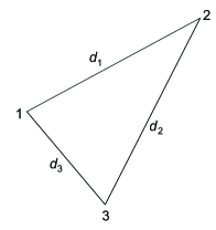
Figure 1: Undirected Triangular Formation

III Error System

Our aim is to study the geometry of the overall system. Towards this end, first note that

$$\dot{z}=-\bar{H}R^{\prime}(z)e(z)+\bar{H}S^{\prime}(z)\mu$$ (9)

because of (4) and (7). This equation and the definitions of the $e_{k}$ in (5) enable one to write

$$\dot{e}=-2R(z)R^{\prime}(z)e+2R(z)S^{\prime}(z)\mu.$$ (10)

If the target formation $\{\mathbb{G},y\}$ is only infinitesimally rigid but not minimally infinitesimally rigid there are further constraints imposed on $e$ stemming from the fact there are geometric dependencies between its components. Because of this, along trajectories where $\{\mathbb{G},x(t)\}$ is infinitesimally rigid, $e$ evolves in a closed proper subset ${\cal E}\subset{\rm I\!R}^{m}$ containing $0$. We now explain what these dependencies are and in the process define ${\cal E}$.

Set $\tilde{m}=2n-3$, the rank of the rigidity matrix of $\{\mathbb{G},y\}$. Suppose that $\{\mathbb{G},y\}$ is not minimally infinitesimally rigid in which case $m>\tilde{m}$. Let $\tilde{\mathbb{G}}$ be any spanning subgraph of $\mathbb{G}$ for which $\{\tilde{\mathbb{G}},y\}$ is minimally infinitesimally rigid. Write $\tilde{e}$ for the sub-vector of $e$ whose $\tilde{m}$ entries are those entries in $e$ corresponding to the edges in $\tilde{\mathbb{G}}$. Similarly, write $\widehat{e}$ for those entries in $e$ corresponding to the $m-\tilde{m}$ edges in $\mathbb{G}$ which have been deleted to form $\tilde{\mathbb{G}}$. Let $\tilde{P}$ and $\widehat{P}$ be those matrices for which $\tilde{e}=\tilde{P}e$ and $\widehat{e}=\widehat{P}e$ respectively. Note that $\left[\begin{matrix}\tilde{P}^{\prime}&\widehat{P}^{\prime}\end{matrix}\right]$ is a permutation matrix; therefore $\tilde{P}\tilde{P}^{\prime}=I$, $\widehat{P}\widehat{P}^{\prime}=I$, $\tilde{P}\widehat{P}^{\prime}=0$, and $e=\tilde{P}^{\prime}\tilde{e}+\widehat{P}^{\prime}\widehat{e}$.

Recall that each entry $e_{s}$ in $e$ is, by definition, a function of the form $(x_{i}-x_{j})^{\prime}(x_{i}-x_{j})-d_{s}^{2}$ where $(i,j)$ is the $s$th edge in $\mathbb{G}$. The following proposition implies that each such $e_{s}$ can be expressed as a smooth function of $\tilde{e}$ at points $x$ in a suitably defined open subset of ${\rm I\!R}^{2n}$ where $\{\tilde{\mathbb{G}},x\}$ is minimally infinitesimally rigid.

Proposition 1

Let $\{\mathbb{G},y\}$ be a target formation. There exists an open subset ${\cal A}\subset{\rm I\!R}^{2n}$ containing $y$ for which the following statements are true. For each four distinct integers $i,j,k,l$ in $\mathbf{n}$, there exists a smooth function $\eta_{ijkl}:\tilde{P}e(\bar{H}{\cal A})\rightarrow{\rm I\!R}$ for which

$$(x_{i}-x_{j})^{\prime}(x_{k}-x_{l})=\eta_{ijkl}(\tilde{P}e(\bar{H}x)),\;\;\;x\in{\cal A}.$$ (11)

Moreover, ${\cal A}$ is invariant under the action of $\mathfrak{G}$ and for each $x\in{\cal A}$, the reduced formation $\{\tilde{G},x\}$, is minimally infinitesimally rigid.

The proof of this proposition will be given at the end of this section.

In view of Proposition 1, there must be a smooth function $\psi:\tilde{P}e(\bar{H}{\cal A})\rightarrow{\rm I\!R}^{(m-\tilde{m})}$ such that $\widehat{e}(\bar{H}x)=\psi(\tilde{P}e(\bar{H}x)),\;\;x\in{\cal A}$. Observe that $\psi(0)=0$ because $\widehat{P}e(\bar{H}y)=\psi(\tilde{P}e(\bar{H}y))$ and $e(\bar{H}y)=0$.

Note that

$$e(\bar{H}x)=\tilde{P}^{\prime}\tilde{e}(\bar{H}x)+\widehat{P}^{\prime}\psi(\tilde{e}(\bar{H}x)),\;\;\;x\in{\cal A}$$ (12)

because $e=\tilde{P}^{\prime}\tilde{e}+\widehat{P}^{\prime}\widehat{e}$. Moreover, since $\widehat{P}\tilde{P}^{\prime}=0$, $\widehat{P}\widehat{P}^{\prime}=I$ and $\tilde{e}=\tilde{P}e$, it must be true that for $x\in{\cal A}$, $\widehat{P}e(\bar{H}x)=\psi(\tilde{P}e(\bar{H}x))$. In other words, for such values of $x$, $e(\bar{H}x)$ takes values in the subset

$${\cal E}=\{e:\widehat{P}e-\psi(\tilde{P}e)=0,\;e\in e(\bar{H}{\cal A})\}.$$

It is easy to see that $0\in{\cal E}$.

We claim that for values of $x(t)\in{\cal A}$, the reduced error $\tilde{e}=\tilde{P}e$ satisfies the differential equation

$$\dot{\tilde{e}}=-2\tilde{R}\tilde{R}^{\prime}\tilde{e}-2\tilde{R}\tilde{R}^{\prime}F^{\prime}(\tilde{e})\psi(\tilde{e})+2\tilde{R}S^{\prime}\mu$$ (13)

where $\tilde{R}(\bar{H}x)$ is the rigidity matrix of the minimally infinitesimally rigid formation $\{\tilde{\mathbb{G}},x\}$ and

$$F(\tilde{e})=\frac{\partial}{\partial\tilde{e}}\psi(\tilde{e}).$$ (14)

To understand why this is so, note first that (10) and (12) imply that

$$\dot{\tilde{e}}=-2\tilde{P}RR^{\prime}(\tilde{P}^{\prime}\tilde{e}+\widehat{P}^{\prime}\psi(\tilde{e}))+2\tilde{P}RS^{\prime}\mu.$$ (15)

By definition, the rigidity matrix of $\{\tilde{\mathbb{G}},x\}$ is $\tilde{R}(\bar{H}x)=\frac{1}{2}\frac{\partial}{\partial x}\tilde{e}(\bar{H}x)$. Clearly $\tilde{P}\frac{1}{2}\frac{\partial}{\partial x}e(\bar{H}x)=\tilde{P}R(\bar{H}x)$ so $\tilde{R}=\tilde{P}R$. From this and (15) it follows that

$$\dot{\tilde{e}}=-2\tilde{R}\tilde{R}^{\prime}\tilde{e}-2\tilde{R}(\widehat{P}R)^{\prime}\psi(\tilde{e})+2\tilde{R}S^{\prime}\mu$$ (16)

But by definition, $R(\bar{H}x)=\frac{1}{2}\frac{\partial}{\partial x}e(\bar{H}x)$. From this and (12) it follows that $R=\tilde{P}^{\prime}\tilde{R}+\widehat{P}^{\prime}F\tilde{R}$ where $F$ is given by (14). Thus $\widehat{P}R=F\tilde{R}$ which justifies the claim that (13) holds.

The preceding easily extends to the case when $\{\mathbb{G},y\}$ itself is minimally infinitesimally rigid. In this case, $\tilde{e}=e$ and (12) holds with $\tilde{P}=I$, $\widehat{P}=0$, and $\psi=0$, while ${\cal E}={\rm I\!R}^{m}$.

The proof of Proposition 1 relies on several geometric facts. The ones we need are encompassed by the following two lemmas.

Lemma 1

Let $v_{1},v_{2},v_{3},v_{4}$ be four vectors in ${\rm I\!R}^{s}$ where $s$ is any fixed positive integer. Then

$$(v_{1}-v_{2})^{\prime}(v_{3}-v_{4})=\frac{1}{2}\{||v_{3}-v_{2}||^{2}+||v_{1}-v_{4}||^{2}-||v_{3}-v_{1}||^{2}-||v_{2}-v_{4}||^{2}\}.$$ (17)

Proof of Lemma 17: Note that

$$(v_{1}-v_{2})^{\prime}(v_{3}-v_{4})=(v_{1}-v_{3})^{\prime}(v_{3}-v_{4})-(v_{2}-v_{3})^{\prime}(v_{3}-v_{4})$$ (18)

because $v_{1}-v_{2}=(v_{1}-v_{3})-(v_{2}-v_{3})$. But

$$(v_{1}-v_{3})^{\prime}(v_{3}-v_{4})=\frac{1}{2}\{||v_{1}-v_{4}||^{2}-||v_{3}-v_{1}||^{2}-||v_{3}-v_{4}||^{2}\}$$

and

$$(v_{2}-v_{3})^{\prime}(v_{3}-v_{4})=\frac{1}{2}\{||v_{2}-v_{4}||^{2}-||v_{3}-v_{2}||^{2}-||v_{3}-v_{4}||^{2}\}.$$

From these identities and (18) it follows that (17) is true.  

In the sequel we will show that for any $x=\left[\begin{matrix}x_{1}^{\prime}&x_{2}^{\prime}&\cdots&x_{n}^{\prime}\end{matrix}\right]^{\prime}$ in a suitably defined open set of multi-points $x$ for which $\{\tilde{\mathbb{G}},x\}$ is minimally infinitesimally rigid, it is possible to express the squared distances between each pair of points $x_{i},x_{j}$ in terms of the reduced error $\tilde{P}e(\bar{H}x)$. Since infinitesimal rigidity demands among other things that for at least one pair of points $p$ and $q$, $x_{p}\neq x_{q}$, nothing will be lost by excluding from consideration at the outset, values of $x$ for which $x_{p}=x_{q}$. For simplicity we will assume the vertices are labeled so that $x_{1}\neq x_{2}$. Accordingly, let ${\cal X}$ denote the set of all $x\in{\rm I\!R}^{2n}$ for which $x_{1}\neq x_{2}$ and write $\delta:{\cal X}\rightarrow{\rm I\!R}^{\frac{n(n-1)}{2}}$ for the squared distance function

$$x\longmapsto\left[\begin{matrix}||x_{1}-x_{2}||^{2}&||x_{1}-x_{3}||^{2}&\cdots&||x_{n-1}-x_{n}||^{2}\end{matrix}\right]^{\prime}.$$

To avoid unnecessarily cluttered formulas in the statements and proofs of some of the lemmas which follow, we will make use of the function $\rho:{\cal X}\rightarrow{\rm I\!R}^{\tilde{m}}$ defined by $x\longmapsto\tilde{P}e(\bar{H}x)$. Note that $\rho(x)$ and $\tilde{P}e(\bar{H}x)$ have the same value at every point $x\in{\cal X}$, although their domains are different; consequently they are different functions. Note also that for any transformation $\gamma$ in the restriction of $\mathfrak{G}$ to ${\cal X}$, $\rho\circ\gamma=\rho$. Thus for any subset ${\cal W}\subset{\cal X}$, $\rho^{-1}({\cal W})$ is $\mathfrak{G}$ invariant.

Lemma 2

Let $\{\mathbb{G},y\}$ be a target formation. There is an open set ${\cal A}\subset{\cal X}$ containing $y$ and a smooth function $f:\tilde{P}e(\bar{H}{\cal A})\rightarrow{\rm I\!R}^{\frac{n(n-1)}{2}}$ for which

$$\delta(x)=f(\tilde{P}e(\bar{H}x)),\;\;x\in{\cal A}.$$ (19)

Moreover, ${\cal A}$ is invariant under the action of $\mathfrak{G}$ and for all $x\in{\cal A}$, the reduced formation $\{\tilde{\mathbb{G}},x\}$ is minimally infinitesimally rigid.

Proof of Lemma 2: For each nonzero vector $q=\left[\begin{matrix}q_{1}&q_{2}\end{matrix}\right]^{\prime}$ in ${\rm I\!R}^{2}$, let $T_{q}$ denote the rotation matrix

$$T_{q}=\frac{1}{||q||}\left[\begin{matrix}q_{2}&-q_{1}\cr q_{1}&q_{2}\end{matrix}\right].$$

Note that $T_{q}q=\left[\begin{matrix}0&||q||\end{matrix}\right]^{\prime}$ and that the function $q\longmapsto T_{q}$ is well-defined and smooth on ${\rm I\!R}^{2}-0$. Next, with $\tilde{m}=2n-3$, write $\pi:{\cal X}\rightarrow{\rm I\!R}^{\tilde{m}}$ for that function which assigns to $x=\left[\begin{matrix}x_{1}^{\prime}&x_{2}^{\prime}&\cdots&x_{n}^{\prime}\end{matrix}\right]^{\prime}\in{\cal X}$, the vector

$$\left[\begin{matrix}||x_{2}-x_{1}||&(T_{(x_{2}-x_{1})}(x_{3}-x_{1}))^{\prime}&\cdots&(T_{(x_{2}-x_{1})}(x_{n}-x_{1}))^{\prime}\end{matrix}\right]^{\prime}$$

in ${\rm I\!R}^{\tilde{m}}$. Note that $\pi$ is well defined and smooth. Clearly

$$||x_{j}-x_{1}||^{2}=||T_{(x_{2}-x_{1})}(x_{j}-x_{1})||^{2},\;\;\;j\in\{3,4,\ldots,n\}$$

and

$$||x_{j}-x_{i}||^{2}=||T_{(x_{2}-x_{1})}(x_{j}-x_{1})-T_{(x_{2}-x_{1})}(x_{i}-x_{1})||^{2},\\ i\in\{2,3,\ldots,n\},\;\;\;j\in\{i+1,,i+2,\ldots,n\}.$$

Thus any entry in $\delta(x)$ is a polynomial function of entries in $\pi(x)$. Therefore there is a polynomial function $\bar{\delta}:{\rm I\!R}^{\tilde{m}}\rightarrow{\rm I\!R}^{\frac{n(n-1)}{2}}$ such that $\delta=\bar{\delta}\circ\pi$. Since same reasoning applies to the error map $\rho$, there must also be a polynomial function $\bar{\rho}:{\rm I\!R}^{\tilde{m}}\rightarrow{\rm I\!R}^{\tilde{m}}$ such that $\rho=\bar{\rho}\circ\pi$.

Note that the derivative of $\frac{1}{2}\rho$ at $y$, namely $\frac{1}{2}\frac{\partial\rho(x)}{\partial x}|_{x=y}$ is the rigidity matrix of reduced formation $\{\tilde{\mathbb{G}},y\}$. Since $\{\tilde{\mathbb{G}},y\}$ is minimally infinitesimally rigid, ${\rm rank\;}\frac{\partial\rho(x)}{\partial x}|_{x=y}=\tilde{m}$. Meanwhile $\frac{\partial\rho(x)}{\partial x}|_{x=y}=\frac{\partial\bar{\rho}(q)}{\partial q}|_{q=\pi(y)}\frac{\partial\pi(x)}{\partial x}|_{x=y}$. Therefore

$${\rm rank\;}\frac{\partial\bar{\rho}(q)}{\partial q}|_{q=\pi(y)}\geq\tilde{m}.$$ (20)

But $\frac{\partial\bar{\rho}(q)}{\partial q}|_{q=\pi(y)}$ is an $\tilde{m}\times\tilde{m}$ matrix so it must be nonsingular. Thus by the inverse function theorem, there is an open subset ${\cal W}\subset{\rm I\!R}^{\tilde{m}}$ containing $\pi(y)$ for which $\bar{\rho}$ has a smooth inverse $\theta:\bar{\rho}({\cal W})\rightarrow{\cal W}$. Therefore $\theta(\bar{\rho}\circ\pi(x))=\pi(x)$ for $\pi(x)\in{\cal W}$ or equivalently

$$\theta(\rho(x))=\pi(x),\;\;\;x\in\pi^{-1}({\cal W}).$$ (21)

Note that the non-singularity of $\frac{\partial\bar{\rho}(q)}{\partial q}$ at $q=\pi(y)$ implies that ${\cal W}$ can be chosen so that (21) holds and at the same time, so that $\frac{\partial\bar{\rho}(q)}{\partial q}$ is nonsingular on ${\cal W}$. Let ${\cal W}$ be so defined.

Set ${\cal A}=\pi^{-1}({\cal W})$ and note that $y\in{\cal A}$ because $\pi(y)\in{\cal W}$. From (21) and the fact that $\delta=\bar{\delta}\circ\pi$ there follows

$$\delta(x)=\bar{\delta}\circ\theta\circ\rho(x),\;\;\;x\in{\cal A}.$$

Since $\rho(x)=\tilde{P}e(\bar{H}x),\;x\in{\cal A}$, (19) holds with $f=\bar{\delta}\circ\bar{\rho}^{-1}$.

The definition of $\pi$ implies that $\pi\circ\gamma$ for all transformations $\gamma$ in the restriction of $\mathfrak{G}$ to ${\cal X}$. This and the definition of ${\cal A}$ imply that ${\cal A}$ is $\mathfrak{G}$ - invariant.

Non-singularity of the matrix $\frac{\partial\bar{\rho}(q)}{\partial q}$ on ${\cal W}$ implies non-singularity of $\frac{\partial\bar{\rho}(q)}{\partial q}|_{q=\pi(x)}$ for $x\in{\cal A}$. Since the rigidity matrix of $\{\tilde{\mathbb{G}},x\}$ at $x\in{\cal A}$ can be written as $\frac{\partial\bar{\rho}(q)}{\partial q}|_{q=\pi(x)}\frac{\partial\pi(x)}{\partial x}$, to establish minimal infinitesimal rigidity of $\{\tilde{\mathbb{G}},x\}$ on ${\cal A}$, it is enough to show that for each $x\in{\cal A}$

$${\rm rank\;}\frac{\partial\pi(x)}{\partial x}\geq\tilde{m}.$$ (22)

By direct calculation

$$\frac{\partial\pi(x)}{\partial x}=\left[\begin{matrix}A_{1\times 4}&0\cr\cr C_{(2n-4)\times 4}&B_{(2n-4)\times(2n-4)}\end{matrix}\right]$$

where $A=\frac{1}{||x1-x_{2}||}\left[\begin{matrix}x_{1}^{\prime}-x_{2}^{\prime}&x_{2}^{\prime}-x_{1}^{\prime}\end{matrix}\right]$, $B={\rm block\;diagonal\;}\{T_{x_{2}-x_{1}},\ldots,T_{x_{2}-x_{1}}\}$ and $C$ is some suitable defined matrix. Moreover $A$ is nonzero because $x\in{\cal X}$ and $B$ is nonsingular because $T_{x_{2}-x_{1}}$ is a rotation matrix. Thus the rows of $\frac{\partial\pi(x)}{\partial x}$ are linearly independent for $x\in{\cal A}$. It follows that (22) holds for all $x\in{\cal A}$ and thus $\{\tilde{\mathbb{G}},x\}$ is minimally infinitesimally rigid for all such $x$  

Proof of Proposition 1: In view of Lemma 2, there exists a $\mathfrak{G}$ - invariant, open set ${\cal A}\subset{\rm I\!R}^{2n}$ containing $y$ and a smooth function $f$ for which (19) holds. Let $i,j,k,l$ be distinct integers in $\mathbf{n}$. In view of Lemma 17, to establish the correctness of statement (11) it is enough to prove the existence of $\eta_{ijkl}$ for the case when $k=i$ and $j=l$. But the existence of $\eta_{ijij}$ follows at once from (19) and the definition of the squared distance function $\delta$. The minimal infinitesimally rigidity of $\{\tilde{\mathbb{G}},x\}$ for $x\in{\cal A}$, follows from Lemma 2.  

III-A Error System Definition

A key step in the analysis of the gradient law proposed in [6] is to show that along trajectories of the overall system (7), the reduced error vector $\tilde{e}$ satisfies a self-contained differential equation of the form $\dot{\epsilon}=g(\epsilon,\mu)$ where $g$ is a smooth function of just $\epsilon$ and $\mu$ and not $z$. As we will see, this can be shown to be true when $x(t)$ takes values in the open subset ${\cal A}$ mentioned in the statement of Proposition 1. The precise technical result is as follows.

Theorem 1

Let $\{\mathbb{G},y\}$ be a target formation and let ${\cal A}$ be the open subset of ${\rm I\!R}^{2n}$ mentioned in the statement of Proposition 1. There exists a smooth function $g:\tilde{P}e(\bar{H}{\cal A})\times{\rm I\!R}^{m}\rightarrow{\rm I\!R}^{\tilde{m}}$ for which

$$g(\tilde{e},\mu)=-2\tilde{R}\tilde{R}^{\prime}\tilde{e}-2\tilde{R}\tilde{R}^{\prime}F^{\prime}(\tilde{e})\psi(\tilde{e})+2\tilde{R}S^{\prime}\mu,\;\;x\in{\cal A}$$ (23)

where $\tilde{e}$ is the reduced error $\tilde{e}=\tilde{P}e(\bar{H}x)$ and $F$ is given by (14). Moreover, if $x(t)$ is a solution to the overall system (7) for which $x(t)\in{\cal A}$ on some time interval $[t_{0},t_{1})$, then on the same time interval, the reduced error vector $\tilde{e}=\tilde{P}e(\bar{H}x(t))$ satisfies the self-contained differential equation

$$\dot{\epsilon}=g(\epsilon,\mu).$$ (24)

Although ${\cal A}$ and $g$ are defined for a specific target formation $\{\mathbb{G},y\}$, it is not difficult to see that both are the same for all formations which are in the same orbit as $\{\mathbb{G},y\}$. In the sequel we refer to (24) as the error system and we say that ${\cal A}$ is the ambient space on which it is valid.

Proof of Theorem 24: The structures previously defined matrices $D(z)={\rm diagonal}\;\{z_{1},z_{2},\ldots,z_{m}\}$, $R(z)=D^{\prime}(z)\bar{H}$, $S(z)=D^{\prime}(z)\bar{J}$ $\tilde{R}(z)=\tilde{P}R(z)$ imply that the entries of both $\tilde{R}(z)\tilde{R}^{\prime}(z)$ and $\tilde{R}(z)S^{\prime}(z)$ are linear functions of the entries of the Gramian $\left[\begin{matrix}z_{1}&z_{2}&\cdots z_{m}\end{matrix}\right]^{\prime}\left[\begin{matrix}z_{1}&z_{2}&\cdots z_{m}\end{matrix}\right]$. In view of (3) it is therefore clear that the entries of $\tilde{R}(z)\tilde{R}^{\prime}(z)|_{z=\bar{H}x}$ and $\tilde{R}(z)S^{\prime}(z)|_{z=\bar{H}x}$ can be written as a linear combination of inner product terms of the form $(x_{i}-x_{j})^{\prime}(x_{k}-x_{l})$ for $i,j,k,l\in\mathbf{n}$. From this and Proposition 1 it is clear that there exists an open subset ${\cal A}\subset{\rm I\!R}^{2n}$ containing $y$ for which each entry in $\tilde{R}(z)\tilde{R}^{\prime}(z)|_{z=\bar{H}x}$ and $\tilde{R}(z)S^{\prime}(z)|_{z=\bar{H}x}$ can be written as a smooth function of $\tilde{P}e(\bar{H}x)$ on $\tilde{P}e(\bar{H}{\cal A})$. The existence of a smooth function for which (23) holds follows at once. The second statement of the theorem is an immediate consequence is this and (13).  .

III-B Exponential Stability of the Unperturbed Error System

In this section we shall study the stability of the error system for the special case when $\mu=0$. It is clear from (23) that in this case, the zero state $\epsilon=0$ is an equilibrium state of the unperturbed error system. The follow theorem states that this is in fact an exponentially stable equilibrium.

Theorem 2

The equilibrium state $\epsilon=0$ of the unperturbed error system $\dot{\epsilon}=g(\epsilon,0)$ is locally exponentially stable.

Proof of Theorem 2: First suppose that the target formation $\{\mathbb{G},y\}$ is not minimally infinitesimally rigid, and that the reduced formation $\{\tilde{\mathbb{G}},y\}$ is. To prove that $\epsilon=0$ is a locally exponentially stable equilibrium it is enough to show that the linearization of $\dot{\epsilon}=g(\epsilon,0)$ at $0$ is exponentially stable [16]. As noted in the proof of Theorem 24, the matrix $\tilde{R}(z)\tilde{R}^{\prime}(z)|_{z=\bar{H}x}$ can be written as a smooth function of $\tilde{P}e(\bar{H}x)$ on $\tilde{P}e(\bar{H}{\cal A})$ Thus the function $Q:\tilde{P}e(\bar{H}{\cal A})\rightarrow{\rm I\!R}^{\tilde{m}\times\tilde{m}}$ for which $Q(\tilde{P}e(\bar{H}x))=\tilde{R}(\bar{H}x)\tilde{R}^{\prime}(\bar{H}x)$ is well defined, smooth, and positive semi-definite on $\tilde{P}e(\bar{H}{\cal A})$. We claim that $Q(0)$ is nonsingular and thus positive definite. To understand why this is so, recall that for any vector $x\in{\rm I\!R}^{2n}$, $\tilde{R}(z)|_{z=\bar{H}x}$ is the rigidity matrix of the formation $\{\tilde{\mathbb{G}},x\}$. In addition, $y\in{\cal A}$ so by Proposition 1, the formation $\{\tilde{\mathbb{G}},y\}$ is minimally infinitesimally rigid. Therefore ${\rm rank\;}\tilde{R}(\bar{H}y)=\tilde{m}$. Hence $\tilde{R}(\bar{H}y)\tilde{R}^{\prime}(\bar{H}y)$ is nonsingular. Moreover $Q(0)=\tilde{R}(\bar{H}y)\tilde{R}^{\prime}(\bar{H}y)$ since $\tilde{e}(\bar{H}y)=0$. Therefore $Q(0)$ is nonsingular as claimed.

From (23), the definition of $Q$, and the definition of $F$ in (14), it is clear that for $\epsilon\in\tilde{P}e(\bar{H}{\cal A})$

$$\frac{\partial g(\epsilon,0)}{\partial\epsilon}=-2Q(I+F^{\prime}F+F^{\prime}\psi)-2\left(\frac{\partial Q}{\partial\epsilon}\right)(\epsilon+F^{\prime}\psi).$$

Therefore

$$\left.\frac{\partial g(\epsilon,0)}{\partial\epsilon}\right|_{\epsilon=0}=-2Q(0)(I+F^{\prime}(0)F(0)).$$ (25)

But $-2Q(0)(I+F^{\prime}(0)F(0))$ is similar to $-2TQ(0)T^{\prime}$ where $T$ is any nonsingular matrix such that $T^{\prime}T=I+F^{\prime}(0)F(0)$. Since $-2TQ(0)T^{\prime}$ is negative definite, it is a stability matrix. Hence $-2Q(0)(I+F^{\prime}(0)F(0))$ is a stability matrix. Therefore the linearization of $\dot{\epsilon}=g(\epsilon,0)$ at $\epsilon=0$ is exponentially stable. Therefore $\epsilon=0$ is an exponentially stable equilibrium of the error system $\dot{\epsilon}=g(\epsilon,0)$.

Now suppose that $\{\mathbb{G},y\}$ itself is minimally infinitesimally rigid. In this case the same argument just used applies except that in this case, the right side of (25) is just $-2Q(0)$.  

III-C Exponential Stability of the Perturbed Error System

As is well known, a critically important property of exponential stability is robustness. We now explain exactly what this means for the error system under consideration. First suppose that the target formation $\{\mathbb{G},y\}$ is not minimally infinitesimally rigid, and that the reduced formation $\{\tilde{\mathbb{G}},y\}$ is.

1. As was just shown in the proof of Theorem 2, (25) holds and $-2Q(0)(I+F^{\prime}(0)F(0))$ is a stability matrix.

2. Clearly $-2Q(0)(I+F^{\prime}(0)F(0))$ is nonsingular. Therefore by the implicit function theorem, there exists an open neighborhood ${\cal M}_{0}\subset{\rm I\!R}^{m}$ centered at $0$ and a vector $\epsilon_{\mu}$ which is a smooth function of $\mu$ on ${\cal M}_{0}$ such that $\epsilon_{0}=0$ and $g(\epsilon_{\mu},\mu)=0$ for $\mu\in{\cal M}_{0}$.

3. The Jacobian matrix

   $$J(\mu)=\frac{\partial g(\epsilon,\mu)}{\partial\epsilon}|_{\epsilon=\epsilon_{\mu}}$$

   in continuous on ${\cal M}_{0}$ and equals the stability matrix $-2Q(0)(I+F^{\prime}(0)F(0))$ at $\mu=0$. For any $\mu$ in any sufficiently small open neighborhood ${\cal M}\subset{\cal M}_{0}$ about $0$, $J(\mu)$ is a stability matrix.

4. Stability of $J(\mu)$ is equivalent to exponential stability of the equilibrium state $\epsilon_{\mu}$ of the system $\dot{\epsilon}=g(\epsilon,\mu)$.

Of course the same arguments apply, with minor modification, to the case when $\{\mathbb{G},y\}$ itself is minimally infinitesimally rigid. We summarize:

Corollary 1

On any sufficiently small open neighborhood ${\cal M}\subset{\rm I\!R}^{m}$ about $\mu=0$, there is a smooth function $\mu\longmapsto\epsilon_{\mu}$ such that $\epsilon_{0}=0$ and for each $\mu\in{\cal M}$, $\epsilon_{\mu}$ is an exponentially stable equilibrium state of the error system $\dot{\epsilon}=g(\epsilon,\mu).$

Prompted by (12), we define the equilibrium output of the error system $\dot{\epsilon}=g(\epsilon,\mu)$ to be $\mathfrak{e}_{\mu}=\tilde{P}^{\prime}\epsilon_{\mu}+\widehat{P}^{\prime}\psi(\epsilon_{\mu})$. As noted just below the statement of Proposition 1, $\psi$ is a smooth function and $\psi(0)=0$. Thus, like the error system’s equilibrium state, $\mathfrak{e}_{\mu}$ is a smooth function of $\mu$ and $\mathfrak{e}_{0}=0$.

III-D Exponential Convergence

At this point we have shown that for $\mu\in{\cal M}$, the equilibrium $\epsilon_{\mu}$ of the error system is locally exponentially stable. We have also shown that along any trajectory of the overall system for which $x(t)\in{\cal A}$, the reduced error $\tilde{e}$ satisfies the error equation (24) and the overall error satisfies (12). It remains to be shown that if $x$ starts out at a value in some suitably defined open subset of ${\cal A}$ for which $\tilde{P}e(\bar{H}x)$ is within the domain of attraction of the error system’s equilibrium $\epsilon_{\mu}$, then $x$ will remain within the subset ${\cal A}$ for all time and consequently $\tilde{e}$ and $e$ and will converge exponentially fast to $\epsilon_{\mu}$ and $\mathfrak{e}_{\mu}=\tilde{P}^{\prime}\epsilon_{\mu}+\widehat{P}^{\prime}\psi(\epsilon_{\mu})$ respectively. This is the subject of Theorem 3 below.

Before stating the theorem we want to emphasize that just because the reduced error might start out at a value $\tilde{P}e(\bar{H}x(0))$ which is close to $\epsilon_{\mu}$ or even equal to $\epsilon_{\mu}$, there is no guarantee that $x(0)$ will be in ${\cal A}$. In fact the only situation when $\tilde{P}e(\bar{H}x(0))=0$ would imply $x\in{\cal A}$ is when the target formation is globally rigid [13]. The complexity of this entire problem can be traced to this point. The problem being addressed here cannot be treated as a standard local stability problem in error space.

Theorem 3

Let $\{\mathbb{G},y\}$ be a target formation and let ${\cal A}$ be the opened set referred to in the statement of Proposition 1. For each value of $\mu$ in any sufficiently small open neighborhood ${\cal M}$ in ${\rm I\!R}^{m}$ about $\mu=0$, and each initial state $x(0)\in{\cal A}$ for which the error $e(\bar{H}x(0))$ is sufficiently close to the equilibrium output $\mathfrak{e}_{\mu}$ of the error system $\dot{\epsilon}=g(\epsilon,\mu)$, the following statements are true:

1. The trajectory of the overall system starting at $x(0)$ exists for all time and lies in ${\cal A}$.

2. The error $e=e(\bar{H}x(t))$ converges exponentially fast to $\mathfrak{e}_{\mu}$.

To prove this theorem, we will need the following lemmas.

Lemma 3

Let $\{\mathbb{G},y\}$ be a target formation and let ${\cal A}$ be the opened set referred to in the statements of Lemma 2 and Proposition 1. There exists an open ball ${\cal B}_{o}\subset{\rm I\!R}^{\tilde{m}}$ centered at $0$ and an open set ${\cal C}\subset{\rm I\!R}^{2n}$ such that ${\cal C}$ and the closure of ${\cal A}$ are disjoint and

$$\rho^{-1}({\cal B}_{o})\subset{\cal A}\cup{\cal C}.$$ (26)

Proof of Lemma 26: Let $\{\mathbb{G},y\},\{\mathbb{G},y^{2}\},\ldots,\{\mathbb{G},y^{n_{o}}\}$ be representative formations within the $n_{o}$ disjoint orbits whose union is the set of all formations equivalent to $\{\mathbb{G},y\}$. By assumption, each of these formations is infinitesimally rigid. Thus by the same reasoning used to establish the existence of ${\cal W}$ and $\theta$ in the proof of Lemma 2, one can conclude that for each $i\in\{2,3,\ldots,n_{o}\}$, there is an open subset ${\cal W}_{i}\subset{\rm I\!R}^{\tilde{m}}$ containing $\pi(y^{i})$ and an inverse function $\theta_{i}:\bar{\rho}({\cal W}_{i})\rightarrow{\cal W}_{i}$. Since the $\pi(y^{i})$ and $\pi(y)$ are distinct points , the ${\cal W}_{i}$ can be assumed to have been chosen small enough so that all are disjoint with the closure of ${\cal W}$. Thus the set ${\cal S}=\cup_{i=2}^{n_{o}}{\cal W}_{i}$ and the closure of ${\cal W}$ are disjoint.

Note that the restriction of $\bar{\rho}$ to ${\cal W}$ is $\theta^{-1}$ which in turn is a homeomorphism. Thus the restriction of $\bar{\rho}$ to ${\cal W}$ is an open function which implies that $\bar{\rho}({\cal W})$ is an opened set. By similar reasoning, each $\bar{\rho}({\cal W}_{i})$ is also an opened set as is the intersection $\cap_{i\in\mathbf{n_{o}}}\bar{\rho}({\cal W}_{i})$ where ${\cal W}_{1}\stackrel{{\scriptstyle\Delta}}{{=}}{\cal W}$. Moreover $0$ is in this intersection because $\pi(y)\in{\cal W}_{1}$, $\pi(y^{i})\in{\cal W}_{i},\;i\in\{2,3,\ldots,n_{o}\}$ and $\bar{\rho}$ maps each of these points into $0$.

Let ${\cal T}$ be the complement of ${\cal W}\cup{\cal S}$ in ${\rm I\!R}^{\tilde{m}}$. Note that $\bar{\rho}({\cal T})$ cannot contain the origin because the only points in the domain of $\bar{\rho}$ which map into $0$ are in ${\cal W}\cup{\cal S}$. This implies that the set

$${\cal B}_{0}=\bigcap_{i\in\mathbf{n_{o}}}\bar{\rho}({\cal W}_{i})-\bar{\rho}({\cal T})\cap\bigcap_{i\in\mathbf{n_{0}}}\bar{\rho}({\cal W}_{i})$$

contains $0$. We claim that ${\cal B}_{0}$ is opened. Since $\cap_{i\in\mathbf{n_{o}}}\bar{\rho}({\cal W}_{i})$ is opened, to establish this, it is enough to show that ${\cal T}\cap\cap_{i\in\mathbf{n_{o}}}\bar{\rho}({\cal W}_{i})$ is closed. This in turn will be true if $\bar{\rho}({\cal T})$ is closed. But this is so because ${\cal T}$ is closed and because $\bar{\rho}$ is a weakly coercive, polynomial function mapping one finite dimensional vector space into another [17].

We claim that

$$\bar{\rho}^{-1}({\cal B}_{o})\subset{\cal W}\cup{\cal S}.$$ (27)

To show that this is so, pick $q\in\bar{\rho}^{-1}({\cal B}_{o})$ in which case $\bar{\rho}(q)\in{\cal B}_{o}$. But $q\subset{\rm I\!R}^{\tilde{m}}$ and ${\rm I\!R}^{\tilde{m}}={\cal W}\cup{\cal S}\cup{\cal T}$ so $q\in{\cal W}\cup{\cal S}\cup{\cal T}$. But $q$ cannot be in ${\cal T}$ because $\bar{\rho}(q)\in{\cal B}_{o}$ and ${\cal B}_{o}$ and $\bar{\rho}({\cal T})$ are disjoint. Thus $\bar{\rho}(q)\in{\cal W}\cup{\cal S}$ so $q\in\bar{\rho}^{-1}({\cal W}\cup{\cal S})$. Therefore (27) is true.

We claim that (26) holds with ${\cal C}=\pi^{-1}({\cal S})$ and that with this choice, ${\cal C}$ and the closure of ${\cal A}$ are disjoint. To establish (26), pick $x\in\rho^{-1}({\cal B}_{o})$; then $\pi(x)\in\bar{\rho}^{-1}({\cal B}_{o})$ because $\rho=\bar{\rho}\circ\pi$. In view of (27), $\pi(x)\in{\cal W}\cup{\cal S}$. But ${\cal A}=\pi^{-1}({\cal W})$ and ${\cal C}=\pi^{-1}({\cal S})$ so $x\in{\cal A}\cup{\cal C}$. Therefore (26) is true.

To complete the proof we need to show that ${\cal C}$ and the closure of ${\cal A}$ are disjoint. Note that because $\pi$ is continuous, $\bar{{\cal A}}\subset\pi^{-1}(\bar{{\cal W}})$ where $\bar{{\cal A}}$ and $\bar{{\cal W}}$ are the closures of ${\cal A}$ and ${\cal W}$ respectively. Then $\bar{{\cal A}}\cap{\cal C}\subset\pi^{-1}(\bar{{\cal W}})\cap\pi^{-1}({\cal S})\subset\pi^{-1}(\bar{{\cal W}}\cap{\cal S})$. But $\bar{{\cal W}}$ and ${\cal S}$ are disjoint so $\bar{{\cal A}}$ and ${\cal C}$ must be disjoint as well.  

Lemma 4

Let $\{\mathbb{G},y\}$ be a target formation and let ${\cal A}$ be the opened set referred to in the statement of Lemma 2 and Proposition 1. For any sufficiently small open ball ${\cal B}\subset{\rm I\!R}^{\tilde{m}}$ centered at $0$,

$${\cal B}\subset\tilde{P}e(\bar{H}{\cal A})$$ (28)

and

$${\rm closure}({\cal A}_{{\cal B}})\subset{\cal A}$$ (29)

where

$${\cal A}_{{\cal B}}=\{x:\tilde{P}e(\bar{H}x)\in{\cal B},\;x\in{\cal A}\}.$$ (30)

Proof of Lemma 30: Since $\rho=\bar{\rho}\circ\pi$, $\rho({\cal A})=\bar{\rho}(\pi({\cal A}))$. Moreover ${\cal A}=\pi^{-1}({\cal W})$; but $\pi$ is surjective so $\pi({\cal A})={\cal W}$. As noted in the proof of Lemma 26, the restriction of $\bar{\rho}$ to ${\cal W}$ is an open map. Since $\rho({\cal A})=\bar{\rho}({\cal W})$ and ${\cal W}$ is opened, $\rho({\cal A})$ must be opened as well. Furthermore, $y\in{\cal A}$ and $\rho(y)=0$, so $0\in\rho({\cal A})$. But by definition, $\tilde{P}e(\bar{H}{\cal A})=\rho({\cal A})$ so $\tilde{P}e(\bar{H}{\cal A})$ is also opened and contains $0$. Thus (28) will hold provided ${\cal B}$ is sufficiently small.

Let ${\cal B}_{0}$ be as in the statement of Lemma 26. Let ${\cal B}$ be any opened ball in ${\rm I\!R}^{\tilde{m}}$ centered at $0$ which is small enough so that its closure $\bar{{\cal B}}$ is contained in ${\cal B}_{0}$. Let $x_{1},x_{2},\ldots,x_{i},\ldots$ be a convergent sequence in ${\cal A}_{{\cal B}}$ with limit $x^{*}$. To establish (29), it is enough to show that $x^{*}\in{\cal A}$. By definition, ${\cal A}_{{\cal B}}={\cal A}\cap\rho^{-1}({\cal B})$ so $x_{i}\in{\cal A}\cap\rho^{-1}({\cal B}),\;i\geq 1$. Therefore $x^{*}\in\bar{{\cal A}}$ which is the closure of ${\cal A}$. Since $x_{i}\in\rho^{-1}({\cal B})$, $\rho(x_{i})\in{\cal B}$. Therefore $\rho(x^{*})\in\bar{{\cal B}}$ so $\rho(x^{*})\in{\cal B}_{o}$. Hence $x^{*}\in\rho^{-1}({\cal B}_{0})$. Thus by Lemma 26, $x^{*}\in{\cal A}\cup{\cal C}$. But $x^{*}\in\bar{{\cal A}}$ and $\bar{{\cal A}}$ and ${\cal C}$ are disjoint so $x^{*}\in{\cal A}$. Therefore (29) is true.  

Proof of Theorem 3: Let ${\cal B}$ be an open ball centered at $0$ which satisfies (28) and (29). Corollary 1 guarantees that for any $\mu$ in any sufficiently small open neighborhood ${\cal M}$ about $0$, the error system has an exponentially stable equilibrium $\epsilon_{\mu}$. Suppose ${\cal M}$ is any such neighborhood, which is also small enough so that for each $\mu\in{\cal M}$, $\epsilon_{\mu}\in{\cal B}$. Since for each $\mu\in{\cal M}$, the error system has $\epsilon_{\mu}$ as an exponentially stable equilibrium, for each such $\mu$ there must be a sufficiently small positive radius $r_{\mu}$ for which any trajectory of the error system starting in $\{\epsilon:||\epsilon-\epsilon_{\mu}||<r_{\mu}\}$, lies wholly within ${\cal B}$ and converges to $\epsilon_{\mu}$ exponentially fast.

Now fix $\mu\in{\cal M}$. We claim that for any point $\epsilon\in{\rm I\!R}^{\tilde{m}}$ such that $||\epsilon-\epsilon_{\mu}||<r_{\mu}$, there is at least one vector $q\in{\cal A}$ for which $\tilde{P}e(\bar{H}q)=\epsilon$. To establish this claim, note first that $\epsilon\in{\cal B}$. In view of (28), there must be a vector $p\in{\cal A}$ such that $\tilde{P}e(\bar{H}p)=\epsilon$. Thus $q=p$ has the required property.

Now let $q$ be any state in ${\cal A}$ such that $e(\bar{H}q)$ is close enough to $\mathfrak{e}_{\mu}$ so that $||\tilde{P}e(\bar{H}q)-\epsilon_{\mu}||<r_{\mu}$. Then $\tilde{P}e(\bar{H}q)\in{\cal B}$ so $q\in{\cal A}_{{\cal B}}$. Let $x(t)$ be the solution to the overall system starting in state $q$. Then $x(0)\in{\cal A}_{{\cal B}}$. Let $[0,T)$ denote the maximal interval of existence for this solution and let $T^{*}$ denote the largest time in this interval such that $x(t)\in{\cal A}_{{\cal B}}$ for $t\in[0,T^{*})$. Suppose $T^{*}<T$ in which case $x(t)$ is well defined on the closed interval $[0,T^{*}]$. Moreover, since $x(t)$ is continuous and in ${\cal A}_{{\cal B}}$ on $[0,T^{*})$ it must be true that $x(t)\in{\rm closure}({\cal A}_{{\cal B}}),\;t\in[0,T^{*}]$. Therefore $x(t)\in{\cal A},\;\;t\in[0,T^{*}]$ because of (29). In view of Theorem 24, $\tilde{P}e(\bar{H}x(t))=\epsilon(t),\;t\in[0,T^{*}]$ where $\epsilon(t)$ is the solution to the error system starting at $\epsilon(0)=\tilde{e}(\bar{H}q)$. But $||\epsilon(0)-\epsilon_{\mu}||<r_{\mu}$, so for $t\in[0,T^{*}]$, $\epsilon(t)\in{\cal B}$. Therefore $\tilde{P}e(\bar{H}x(t))\in{\cal B}$ for $t\in[0,T^{*}]$. It follows that $x(t)\in{\cal A}_{{\cal B}},\;t\in[0,T^{*}]$. This contradicts the hypothesis that $T^{*}$ is the largest time such that $x(T^{*})\in{\cal A}_{{\cal B}}$ for $t<T^{*}$. Therefore $T^{*}=T$. Clearly $\tilde{P}e(\bar{H}x(t))=\epsilon(t)$ and $x(t)\in{\cal A}_{{\cal B}}$ for all $t\in[0,T)$.

The definition of $r_{\mu}$ and the assumption that $||\epsilon(0)-\epsilon_{\mu}||<r_{\mu}$ imply that $\epsilon(t)$ must converge to $\epsilon_{\mu}$ exponentially fast. Thus there must be a positive constant $c$ such that $||\epsilon(t)||\leq c,\;t\geq 0$. Therefore $||\tilde{P}e(\bar{H}x(t))||\leq c,\;t\in[0,T)$. In view of (12), $||e(\bar{H}x(t))||\leq\bar{c}$ where $\bar{c}=||\tilde{P}^{\prime}||c+||\widehat{P}^{\prime}||\sup_{||\zeta||\leq c}||\psi(\zeta)||$. Clearly $||e_{k}(z(t))||\leq\bar{c},\;\;k\in\mathbf{m}$. Therefore $||z_{k}(t)||\leq\sqrt{\bar{c}+d^{2}_{k}},\;\;\;k\in\mathbf{m}$ because of (5). Therefore $||z(t)||$ must be bounded on $[0,T)$ by a constant $C$ depending only on $\bar{c}$ and the $d_{k}$. Since $\dot{x}=-R^{\prime}(z)e(z)+S^{\prime}(z)\mu$ and $R(\cdot)$ and $S(\cdot)$ are continuous, it must be true that $||\dot{x}||$ is bounded on $[0,T)$ by a finite constant. This implies that $||x(t)||\leq c_{1}+c_{2}T,\;t\in[0,T)$ where $c_{1}$ and $c_{2}$ are constants. From this it follows by a standard argument that $T=\infty$. Therefore statement 1 of the theorem is true. Statement 2 is a consequence of (12) and the fact that $\tilde{P}e(\bar{H}x(t))=\epsilon(t),\;t\geq 0$.  

The proof of Theorem 3 makes it clear that if the overall system starts out in a state $x(0)\in{\cal A}$ for which the error $e(\bar{H}x(0))$ is sufficiently close to the error system equilibrium output $\mathfrak{e}_{\mu}$, then the trajectory of the overall system lies wholly with ${\cal A}_{{\cal B}}$ for all time. Repeated use of this fact will be made throughout the remainder of this paper.

IV Square Subsystem

In this section we derive a special $2\times 2$ “square” sub-system whose behavior along trajectories of the overall system will enable us to easily predict the behavior of $x(t)$. Suppose that during some time period $[t_{0},t_{1})$, the state $x(t)$ of the overall system is “close” to a state $y$ for which $\{\mathbb{G},y\}$ is a target formation. Since sufficient closeness of $x(t)$ and $y$ would mean that the formation in $\{\mathbb{G},x(t)\}$ is infinitesimally rigid, it is natural to expect that if $x(t)$ and $y$ are close enough during the period $[t_{0},t_{1})$, then over this period the behavior of all of the $z_{i}$ will depend on only a few of the $z_{i}$. As we will soon see, this is indeed the case. To explain why this is so, we will make use of the fact that the $z$ system in (9) can also be written as

$$\left[\begin{matrix}\dot{z}_{1}&\dot{z}_{2}&\cdots&\dot{z}_{m}\end{matrix}\right]=\left[\begin{matrix}z_{1}&z_{2}&\cdots&z_{m}\end{matrix}\right]M(e(z),\mu)$$ (31)

where $M(e,\mu)$ is a $m\times m$ matrix depending linearly on the pair $(e,\mu)$. This is a direct consequence of the definition of the $z_{i}$ in (3) and the fact that the $x_{i}$ satisfy (6). We can now state the following proposition.

Proposition 2

Let $\{\mathbb{G},y\}$ be a target formation. There are integers $p,q\in\mathbf{m}$ depending on $y$ for which $z_{p}(y)$ and $z_{q}(y)$ are linearly independent. Moreover, for any ball ${\cal B}$ about zero which satisfies (28) and (29), the matrix $Z(z)=\left[\begin{matrix}z_{p}&z_{q}\end{matrix}\right]$ is nonsingular on $\bar{H}{\cal A}_{{\cal B}}$ and there is a smooth matrix - valued function $Q:e(\bar{H}{\cal A}_{{\cal B}})\rightarrow{\rm I\!R}^{2\times m}$ for which

$$\left[\begin{matrix}z_{1}&z_{2}&\ldots&z_{m}\end{matrix}\right]=Z(z)Q(e(z)),\;\;z\in\bar{H}{\cal A}_{{\cal B}}.$$ (32)

If $x(t)$ is a solution to the overall system (7) for which $x(t)\in{\cal A}_{{\cal B}}$ on some time interval $[t_{0},t_{1})$, then on the same time interval, $Z(\bar{H}x(t))$ is nonsingular and satisfies

$$\dot{Z}=ZA(e(z),\mu)$$ (33)

where $A(e,\mu)=Q(e)M(e,\mu)L$ and $L$ is the $m\times 2$ matrix whose columns are the $p$th and $q$th unit vectors in ${\rm I\!R}^{m}$. Moreover

$$Q(\mathfrak{e}_{\mu})M(\mathfrak{e}_{\mu},\mu)=A(\mathfrak{e}_{\mu},\mu)Q(\mathfrak{e}_{\mu})$$ (34)

where $\mathfrak{e}_{\mu}$ is the equilibrium output of the error system.

The proposition clearly implies that on the time interval $[t_{0},t_{1})$, the behavior of the entire vector $z$ is determined by the behavior of the square subsystem defined by (32) and (33). The proof of Proposition 2 depends on Lemma 5 which we state below.

In the sequel we write $p_{1}\wedge p_{2}$ for the wedge product $p_{1}\wedge p_{2}=\det\left[\begin{matrix}p_{1}&p_{2}\end{matrix}\right]$ of any two vectors $p_{1},p_{2}\in{\rm I\!R}^{2}$. The wedge product is a bilinear map.

Lemma 5

Let $\{\mathbb{G},x\}$ be an infinitesimally rigid formation in ${\rm I\!R}^{2}$ with multi-point $x=\left[\begin{matrix}x^{\prime}_{1}&x^{\prime}_{2}&\cdots&x^{\prime}_{n}\end{matrix}\right]^{\prime}$. Then for at least one pair of edges $(i,k)$ and $(j,k)$ in $\mathbb{G}$ which share a common vertex $k$, $(x_{i}-x_{k})\wedge(x_{j}-x_{k})\neq 0$.

A proof of this lemma is given in the appendix.

Proof of Proposition 2: Since $\{\mathbb{G},y\}$ is a target formation, it is infinitesimally rigid. In view of Lemma 5 and the definition of $z_{i}$ in (3), there exist integers $p,q\in\mathbf{m}$ for which $z_{p}\wedge z_{q}\neq 0$ at $x=y$. By a simple computation

$$(z_{p}\wedge z_{q})^{2}=||z_{p}||^{2}||z_{q}||^{2}-(z_{p}^{\prime}z_{q})^{2}$$ (35)

for all $x$. Suppose that $x_{i},x_{j},x_{k},x_{l}$ are the sub-vectors of $x$ for which $z_{p}=x_{i}-x_{j}$ and $z_{q}=x_{k}-x_{l}$. As a consequence of (35) and Proposition 1 there is a smooth function $h:e(\bar{H}{\cal A})\rightarrow{\rm I\!R}$ such that $(z_{p}\wedge z_{q})^{2}=h(e(\bar{H}x)),\;x\in{\cal A}$; moreover $h(e(\bar{H}y))\neq 0$ because $z_{p}(y)\wedge z_{q}(y)\neq 0$. It follows that $z_{p}\wedge z_{q}\neq 0,\;x\in{\cal A}_{{\cal B}}$. Thus $z_{p}\wedge z_{q}\neq 0$ for all $z\in\bar{H}{\cal A}_{{\cal B}}$ so the matrix $Z(z)=\left[\begin{matrix}z_{p}&z_{q}\end{matrix}\right]$ is nonsingular for all such $z$.

To proceed, note that for all $z\in\bar{H}{\cal A}_{{\cal B}}$, the matrix

$$P(z)=\left[\begin{matrix}z_{p}&z_{q}\end{matrix}\right]^{-1}\left[\begin{matrix}z_{1}&z_{2}&\cdots&z_{m}\end{matrix}\right]$$

satisfies

$$\left[\begin{matrix}z_{1}&z_{2}&\cdots&z_{m}\end{matrix}\right]=\left[\begin{matrix}z_{p}&z_{q}\end{matrix}\right]P(z).$$

We claim that for $z\in\bar{H}{\cal A}_{{\cal B}}$, $P(z)$ depends only on $e(z)$; that is $P(z)=Q(e(z))$ for some matrix $Q$ which is a smooth function of $e$. To establish this claim, note first that $P(z)$ can be written at

$$P(z)=\left[\begin{matrix}z_{p}&z_{q}\end{matrix}\right]^{-1}(K\left[\begin{matrix}z_{p}&z_{q}\end{matrix}\right])(K\left[\begin{matrix}z_{p}&z_{q}\end{matrix}\right])^{-1}\cdot\left[\begin{matrix}z_{1}&z_{2}&\ldots&z_{m}\end{matrix}\right]$$

where $K=\left[\begin{matrix}0&-1\cr 1&0\end{matrix}\right]$. By Cramer’s rule

$$(KZ)^{-1}\left[\begin{matrix}z_{1}&z_{2}&\dots&z_{m}\end{matrix}\right]=\frac{1}{z_{p}\wedge z_{q}}\left[\begin{matrix}z_{1}\wedge(Kz_{q})&z_{2}\wedge(Kz_{q})&\cdots&z_{m}\wedge(Kz_{q})\cr(Kz_{p})\wedge z_{1}&(Kz_{p})\wedge z_{2}&\cdots&(Kz_{p})\wedge z_{m}\end{matrix}\right]$$

and

$$Z^{-1}(KZ)=\frac{1}{z_{p}\wedge z_{q}}\left[\begin{matrix}(Kz_{p})\wedge z_{q}&(Kz_{q})\wedge z_{q}\cr z_{p}\wedge(Kz_{p})&z_{p}\wedge(Kz_{q})\end{matrix}\right].$$

But for all $i,j\in\mathbf{m}$, $z_{i}\wedge(Kz_{j})=z_{i}^{\prime}z_{j}$ and $(Kz_{i})\wedge z_{j}=-z_{i}^{\prime}z_{j}$. From this and (35) it follows that

$$P(z)=\frac{1}{(||z_{p}||^{2}||z_{q}||^{2}-(z_{p}^{\prime}z_{q})^{2})}\left[\begin{matrix}z_{p}^{\prime}z_{q}&z_{q}^{\prime}z_{q}\cr-z_{p}^{\prime}z_{p}&-z_{p}^{\prime}z_{q}\end{matrix}\right]\left[\begin{matrix}-z_{1}^{\prime}z_{q}&-z_{2}^{\prime}z_{q}&\cdots&-z_{m}^{\prime}z_{q}\cr z_{p}^{\prime}z_{1}&z_{p}^{\prime}z_{2}&\cdots&z_{p}^{\prime}z_{m}\end{matrix}\right]$$

Since $||z_{p}||^{2}||z_{q}||^{2}-(z_{p}^{\prime}z_{q})^{2}\neq 0,z\in\bar{H}{\cal A}_{{\cal B}}$, $P(z)$ is a smooth function of terms of the form $z_{r}^{\prime}z_{s},\;r,s\in\mathbf{m}$.

In view of (3) it is therefore clear that on ${\cal A}_{{\cal B}}$, $P(\bar{H}x)$ is a smooth function of inner products of the form $(x_{i}-x_{j})^{\prime}(x_{k}-x_{l})$ for $i,j,k,l\in\mathbf{n}$. But ${\cal A}_{{\cal B}}\subset{\cal A}$. From this and Proposition 1 it therefore follows that on ${\cal A}_{{\cal B}}$, $P(\bar{H}x)=Q(e(\bar{H}x))$ where on $e(\bar{H}{\cal A}_{{\cal B}})$, $Q(e)$ is a smooth function of $e$. Thus the claim is established and (32) is true. Moreover, since $x(t)\in{\cal A}_{{\cal B}}$ for $t\in[t_{0},t_{1})$, $z\in\bar{H}{\cal A}_{{\cal B}}$ on the same time interval. Therefore $Z$ is nonsingular on $[t_{0},t_{1}$).

The definition of $L$ implies that

$$Z=\left[\begin{matrix}z_{1}&z_{2}&\ldots&z_{m}\end{matrix}\right]L.$$ (36)

Thus from (31),

$$\dot{Z}=\left[\begin{matrix}z_{1}&z_{2}&\ldots&z_{m}\end{matrix}\right]M(e,\mu)L.$$ (37)

This and (32) imply that (33) is true.

To prove (34), let $x(t)$ be a solution to the overall system in ${\cal A}$, along which $e(\bar{H}x)=\mathfrak{e}_{\mu}$. In view of Theorem 3, such a solution exists. Moreover $x(t)\in{\cal A}_{{\cal B}},\;t\geq 0$. Clearly $z(t)\in\bar{H}{\cal A}_{{\cal B}},\;t\geq 0$ so

$$\left[\begin{matrix}z_{1}&z_{2}&\ldots&z_{m}\end{matrix}\right]=Z(z)Q(\mathfrak{e}_{\mu}),\;t\geq 0$$ (38)

because of (32). We claim that

$$\ker Q(\mathfrak{e}_{\mu})\subset\ker Q(\epsilon_{\mu})M(\mathfrak{e}_{\mu},\mu).$$ (39)

To prove this claim, let $p$ be any vector such that $Q(\mathfrak{e}_{\mu})p=0$. Then $ZQ(\mathfrak{e}_{\mu})p=0,\;t\geq 0$  so

$$\left[\begin{matrix}z_{1}&z_{2}&\ldots&z_{m}\end{matrix}\right]p=0,\;t\geq 0$$

because of (38). Therefore

$$\left[\begin{matrix}\dot{z}_{1}&\dot{z}_{2}&\cdots&\dot{z}_{m}\end{matrix}\right]p=0,\;t\geq 0$$

so

$$\left[\begin{matrix}z_{1}&z_{2}&\ldots&z_{m}\end{matrix}\right]M(\mathfrak{e}_{\mu},\mu)p=0,\;t\geq 0$$

because of (31). Hence by (38), $ZQ(\mathfrak{e}_{\mu})M(\mathfrak{e}_{\mu},\mu)p=0,\;t\geq 0$. But $Z$ is nonsingular for $t\geq 0$, so $Q(\mathfrak{e}_{\mu})M(\mathfrak{e}_{\mu},\mu)p=0$. Since $p$ is arbitrary, (39) is true.

In view of (39), there must be a matrix $B$ such that $Q(\mathfrak{e}_{\mu})M(\mathfrak{e}_{\mu},\mu)=BQ(\mathfrak{e}_{\mu})$ But from (36) and (32) we see that $Z=ZQL$. Since $Z$ is nonsingular, $QL=I_{2\times 2}$. Thus $Q(\mathfrak{e}_{\mu})M(\mathfrak{e}_{\mu},\mu)L=BQ(\mathfrak{e}_{\mu})L=B$, so $B=A(\mathfrak{e}_{\mu},\mu)$.  

V Analysis of the Overall System

In view of Theorem 3, we now know that for any mismatch error $\mu$ with small norm and any initial state $x(0)\in{\cal A}$ for which $e(\bar{H}x(0))$ is close to the error system equilibrium output $\mathfrak{e}_{\mu}$, the error signal $e(\bar{H}x(t))$ must converge exponentially fast to $\mathfrak{e}_{\mu}$ and $\dot{x}(t)$ must be bounded on $[0,\infty)$. But what about $x(t)$ itself? The aim of the remainder of this paper is to answer this question. We will address the question in two steps. First in Section V-A we will consider the situation when $e(\bar{H}x(t))$ has already converged $\mathfrak{e}_{\mu}$. Then in Section V-B we will elaborate on the case when $e(\bar{H}x(t))$ starts out close to $\mathfrak{e}_{\mu}$.

V-A Equilibrium Analysis

The aim of this section is to determine the behavior of the formation $\{\mathbb{G},x(t)\}$ over time for $x(t)\in{\cal A}$ and for mismatch errors from a suitably defined “generic” set, assuming that for each such value of $\mu$, the error $e(\bar{H}x(t))$ is constant and equal to the equilibrium output $\mathfrak{e}_{\mu}$ of the error system. We will do this by first determining in Section V-A1, a set of values of $\mu$ for which $z$ and $x$ are nonconstant for all $t\geq 0.$ Then in Section V-A2 we will show that for such values of $\mu$, the distorted but infinitesimally rigid formation $\{\mathbb{G},x(t)\}$ moves in a circular orbits about the origin in ${\rm I\!R}^{2}$ at a fixed angular speed $\omega_{\mu}$.

V-A1 Mismatch Errors for which $z$ is Nonconstant

The aim of this sub-section is to show that once the error $e(\bar{H}x(t))$ has converged to a constant value, neither $z$ nor $x$ will be constant for small $||\mu||$ other than possibly for certain exceptional values. We shall do this assuming that the target formation $\{\mathbb{G},y\}$ is “unaligned” where by an unaligned formation is meant a formation $\{\mathbb{G},x\}$ with multi-point $x=\left[\begin{matrix}x_{1}^{\prime}&x_{2}^{\prime}&\cdots x_{n}^{\prime}\end{matrix}\right]^{\prime}\in{\rm I\!R}^{2n}$ which does not contain a set of points $x_{i},x_{j},x_{k},x_{l}$ in ${\rm I\!R}^{2}$ for which the line between $x_{i}$ and $x_{j}$ is parallel to the line between $x_{k}$ and $x_{l}$. This is equivalent to saying that $\{\mathbb{G},x\}$ is unaligned if, for every set of four points $x_{i},x_{j},x_{k},x_{l}$ within $x$, $(x_{i}-x_{j})\wedge(x_{k}-x_{l})\neq 0$. It is clear that the set of multi-points $x$ for which $\{\mathbb{G},x\}$ is unaligned is open and dense in ${\rm I\!R}^{2n}$.

Throughout this sub-section we assume that ${\cal A}_{{\cal B}}$ is as in Lemma 30, that ${\cal M}$ is as in Theorem 3 and that for each $\mu\in{\cal M}$, $x(t,\mu)$ is a solution in ${\cal A}_{{\cal B}}$ to the overall system for which $e(\bar{H}x(t,\mu))=\mathfrak{e}_{\mu}$ where $\mathfrak{e}_{\mu}$ is the equilibrium output of the error system $\dot{\epsilon}=g(\epsilon,\mu)$. Our ultimate goal is to show that $z$ is nonconstant for small normed but otherwise “generic” values of $\mu$. The following Proposition enables us to make precise what is meant by a generic value.

Proposition 3

If the target formation $\{\mathbb{G},y\}$ is unaligned, there is an open set ${\cal M}_{0}\subset{\cal M}$ about $\mu=0$ within which the set of values of $\mu$ for which $z(x(t,\mu))$ is nonconstant along an overall system solution $x(t)$ in ${\cal A}_{{\cal B}}$ for which $e(\bar{H}x(t))=\mathfrak{e}_{\mu}$ is open and dense in ${\cal M}_{0}$.

What the proposition is saying is that for almost any value of $\mu$ within any sufficiently small open subset of ${\rm I\!R}^{m}$ which contains the origin, $z(x(t,\mu))$ will be nonconstant along any trajectory of the overall system in ${\cal A}$ for which $e$ is fixed at the equilibrium output $\mathfrak{e}_{\mu}$ of the error system. Thus if $\mu$ has a sufficiently small norm and otherwise chosen at random, it is almost for certain that $z(x(t,\mu))$ will be nonconstant. It is natural to say that $\mu$ is generic, if it is a value in ${\cal M}_{0}$ for which $z(x(t,\mu))$ is nonconstant.

The proof of Proposition 3 relies on a number of ideas. We begin with the following construction which provides a partial characterization of the values of $\mu$ for which $z$ is nonconstant.

Let $x=\left[\begin{matrix}x_{1}^{\prime}&x_{2}^{\prime}&\cdots&x_{n}^{\prime}\end{matrix}\right]^{\prime}$ be any multi-point at which $\{\mathbb{G},x\}$ is an infinitesimally rigid formation. As is well known, the corresponding rigidity matrix $R=R(z)|_{z=\bar{H}x}$ has a kernel of dimension three [1]. We’d like to compute an orthogonal basis for $\ker R$. Towards this end, first recall that rank $H_{m\times n}=n-1$ because $\mathbb{G}$ is a connected graph; thus $\ker H$ must be a one dimensional subspace and because of this $\ker\bar{H}$ must be of dimension two. It is well known and easy to verify that the vectors $q_{1}=\left[\begin{matrix}1&0&1&0&\cdots&1&0\end{matrix}\right]^{\prime}$ and $q_{2}=\left[\begin{matrix}0&1&0&1&\cdots&0&1\end{matrix}\right]^{\prime}$ constitute an orthogonal basis for $\ker\bar{H}$. Next recall that $R=D^{\prime}\bar{H}$. This implies that $q_{1}$ and $q_{2}$ are in $\ker R$. It is easy to verify that a third linearly independent vector in $\ker R$ is $q_{3}=\left[\begin{matrix}(Kx_{1})^{\prime}&(Kx_{2})^{\prime}&\cdots&(Kx_{n})^{\prime}\end{matrix}\right]^{\prime}$ where $K=\left[\begin{matrix}0&-1\cr 1&0\end{matrix}\right]$.

To proceed, let

$$v_{\rm avg}(x)=\frac{1}{n}\sum_{i=1}^{n}x_{i}$$

and define $q_{0}=q_{3}+v_{2}q_{1}-v_{1}q_{2}$ where $\left[\begin{matrix}v_{1}&v_{2}\end{matrix}\right]^{\prime}=v_{\rm avg}(x)$. Since span $\{q_{0},q_{1},q_{2}\}$ and span $\{q_{1},q_{2},q_{3}\}$ are clearly equal, the set $\{q_{0},q_{1},q_{2}\}$ must be a basis for $\ker R$. By direct calculation, $q_{0}^{\prime}q_{i}=0,\;i\in\{1,2\}$, which means that $\{q_{0},q_{1},q_{2}\}$ must be an orthogonal set. Therefore $\{q_{0},q_{1},q_{2}\}$ is an orthogonal basis for $\ker R$. With this basis in hand we can now give an explicit necessary and sufficient condition for $\dot{z}(\bar{H}x(t,\mu))$ to equal zero at any value of $x$ along a trajectory $x(t,\mu),\;t\geq 0$ in ${\cal A}$ of the overall system at which $\dot{e}(\bar{H}x(t,\mu))|_{x(t,\mu)=x}=0$.

Lemma 6

Let $\mu\in{\rm I\!R}^{m}$ be fixed and for $k\in\mathbf{m}$, let $(i_{k},j_{k})$ denote the arc from vertex $i_{k}$ to vertex $j_{k}$ which corresponds to edge $k$ in the oriented graph $\mathbb{G}$. Suppose that multi-point $x=\left[\begin{matrix}x^{\prime}_{1}&x^{\prime}_{2}&\cdots&x^{\prime}_{n}\end{matrix}\right]^{\prime}$ is a state of the overall system along a trajectory in ${\cal A}$ at which

$$\dot{e}(\bar{H}x(t,\mu))|_{x(t,\mu)=x}=0$$

Then at this value of $x$, $\dot{z}(\bar{H}x(t,\mu))|_{x(t,\mu)=x}=0$ if and only if

$$w(x)^{\prime}\mu=0$$ (40)

where

$$w(x)=\left[\begin{array}[]{c}(x_{i_{1}}-v_{\rm avg}(x))\wedge(x_{j_{1}}-v_{\rm avg}(x))\\ \vdots\\ (x_{i_{m}}-v_{\rm avg}(x))\wedge(x_{j_{m}}-v_{\rm avg}(x))\\ \end{array}\right].$$ (41)

The reason why this lemma only partially characterizes the values of $\mu$ for which $z$ is nonconstant, is because the state $x$ in (40) depends on $\mu$. The proof of this lemma is given in the appendix.

Triangle Example Continued: Equation (40) simplifies considerably in the case of a triangular formation. For such a formation with coordinate vectors $x_{1},x_{2},x_{3}$, we can always assume {without loss of generality} a graph orientation for which $x_{i_{3}}=x_{1}=x_{j_{1}}$, $x_{i_{1}}=x_{2}=x_{j_{2}}$ and $x_{i_{2}}=x_{3}=x_{j_{3}}$. Under these conditions it is easy to check that for $k\in\{1,2,3\}$,

$$(x_{i_{k}}-v_{\rm avg}(x))\wedge(x_{j_{k}}-v_{\rm avg}(x))=\frac{1}{3}(x_{2}-x_{1})\wedge(x_{1}-x_{3}).$$

Thus for this example, $\dot{z}(\bar{H}x(t))|_{x(t)=x}=0$ if and only if

$$(x_{2}-x_{1})\wedge(x_{1}-x_{3})(\mu_{1}+\mu_{2}+\mu_{3})=0$$ (42)

where $\left[\begin{matrix}\mu_{1}&\mu_{2}&\mu_{3}\end{matrix}\right]^{\prime}=\mu$.

We now return to the development of ideas needed to prove Proposition 3.

Lemma 7

Let ${\cal B}$ and ${\cal A}_{{\cal B}}$ be as in the statement of Lemma 30. Let $p,q$ be distinct integers in $\mathbf{m}$. There is a continuous function $\alpha:{\cal B}\rightarrow{\rm I\!R}$ for which

$$(x_{p}-v(x))\wedge(x_{q}-v(x))=\alpha(e(\bar{H}x)),\;\;\;x\in{\cal A}_{{\cal B}}$$ (43)

where $v(x)$ is any fixed linear combination of the position vectors $x_{i},\;i\in\mathbf{n}$ in $x$. If, in addition, the target formation $\{\mathbb{G},y\}$ is unaligned, then $\alpha(0)\neq 0$. Moreover, if ${\cal B}$ is sufficiently small, then $\alpha$ is continuously differentiable.

A proof of this lemma is given in the appendix.

Lemma 8

Let ${\cal S}\subset{\rm I\!R}^{m}$ be an open subset containing the origin. Let $f:{\cal S}\rightarrow{\rm I\!R}^{1\times m}$ be a continuously differentiable function such that $f(0)\neq 0$. Then there exists an open neighborhood ${\cal U}\subset{\cal S}$ of the origin within which the set of $s$ for which $f(s)s\neq 0$ is open and dense in $\cal U$.

A proof of this lemma is given in the appendix.

Proof of Proposition 3: Let $w(\cdot)$ be as in the statement of Lemma 41. By hypothesis, $\{\mathbb{G},y\}$ is an unaligned formation and $x(t,\mu)\in{\cal A}_{{\cal B}}$ for all $t\geq 0$ and all $\mu\in{\cal M}$. In view of Lemma 7, for ${\cal B}$ sufficiently small the $\;i$th term in the row vector $w(x(t,\mu))$ can be written as $\alpha_{i}(e(\bar{H}x(t,\mu)))$ where $\alpha_{i}:{\cal B}\rightarrow{\rm I\!R}$ is a continuously differentiable function satisfying $\alpha_{i}(0)\neq 0$. Since this is true for all $m$ terms in $w$, there must be a continuously differentiable function $\beta:{\cal B}\rightarrow{\rm I\!R}^{1\times m}$ satisfying $\beta(0)\neq 0$ for which $w(x(t,\mu))=\beta(e(\bar{H}x(t,\mu))),\;t\geq 0,\;\mu\in{\cal M}$. But $e(\bar{H}x(t,\mu))=\mathfrak{e}_{\mu},\;\;t\geq 0,\;\mu\in{\cal M}$ where $\mathfrak{e}_{0}=0$ and $\mu\longmapsto\mathfrak{e}_{\mu}$ is continuously differentiable. Thus there is a continuously differentiable function $f:{\cal M}\rightarrow{\rm I\!R}^{1\times m}$ for which $f(0)\neq 0$ and $w(x(t,\mu))=f(\mu),\;t\geq 0,\;\mu\in{\cal M}$.

Note that $\dot{e}(\bar{H}x(t,\mu))=0$ because $e(\bar{H}x(t,\mu))=\mathfrak{e}_{\mu}$. Therefore, according to Lemma 41, $\dot{z}(\bar{H}x(t,\mu))=0$ for some $t$ and $\mu\in{\cal M}$ if and only if $w(x(t,\mu))\mu=0$. But $w(x(t,\mu))\mu=f(\mu)\mu$ for all $t\geq 0$. Therefore $z(x(t,\mu))$ is constant for all $t\geq 0$ if and only if $f(\mu)\mu=0$. But by Lemma 8, there exists a neighborhood ${\cal M}_{0}\subset{\cal M}$ of the origin within which the set of $\mu$ for which $f(\mu)\mu\neq 0$ is open and dense in ${\cal M}_{0}$. Thus for any $\mu$ in an open dense subset of ${\cal M}_{0}$, $z(x(t,\mu))$ is nonconstant on $[0,\infty)$  

V-A2 Equilibrium Solutions

The aim of this section is to discuss the evolution of the formation $\{\mathbb{G},x(t,\mu)\}$ along an “equilibrium solution” to the overall system assuming that $\mu$ is fixed at any value in ${\cal M}$. By an equilibrium solution, written $\bar{x}(t)$, is meant any solution to (7) in ${\cal A}$ for which $e(\bar{H}\bar{x}(t))=\mathfrak{e}_{\mu},\;t\geq 0$, where $\mathfrak{e}_{\mu}$ is the equilibrium output of the error system. For simplicity we write $\bar{z}(t)$ for = $z(\bar{x}(t))$ and let $\bar{z}_{i}(t),\;i\in\mathbf{m}$, be the sub-vectors in ${\rm I\!R}^{2}$ comprising $\bar{z}(t)$; i.e., $\bar{z}(t)=\left[\begin{matrix}\bar{z}_{1}^{\prime}(t)&\bar{z}_{2}^{\prime}(t)&\cdots&\bar{z}^{\prime}_{n}(t)\end{matrix}\right]^{\prime}$.

Note that since $e(\bar{H}\bar{x}(t))\in{\cal B}$, $\bar{x}(t)\in{\cal A}_{{\cal B}}$ and therefore $\bar{z}(t)\in\bar{H}{\cal A}_{{\cal B}},\;t\geq 0$. Thus, in view of Proposition 2, there are integers $p,q\in\mathbf{m}$ for which the matrix $\bar{Z}(t)=\left[\begin{matrix}\bar{z}_{p}(t)&\bar{z}_{q}(t)\end{matrix}\right]$ is nonsingular for $t\geq 0$. Moreover

$$\left[\begin{matrix}\bar{z}_{1}&\bar{z}_{2}&\ldots&\bar{z}_{m}\end{matrix}\right]=\bar{Z}(t)\bar{Q},\;\;t\geq 0$$ (44)

and

$$\dot{\bar{Z}}=\bar{Z}\bar{A},\;\;t\geq 0$$ (45)

where $\bar{Q}$ and $\bar{A}$ are the constant matrices $\bar{Q}=Q(\mathfrak{e}_{\mu})$ and $\bar{A}=A(\mathfrak{e}_{\mu},\mu)$. It follows that the Gramian $\bar{Z}^{\prime}\bar{Z}$ must satisfy

$$\dot{\bar{Z}^{\prime}\bar{Z}}=\bar{A}^{\prime}\bar{Z}^{\prime}\bar{Z}+\bar{Z}^{\prime}\bar{Z}\bar{A}.$$ (46)

In view of the definition of the $z_{i}$ in (3), we see that the four entries in $\bar{Z}^{\prime}\bar{Z}$ are of the form $(\bar{x}_{i}(t)-\bar{x}_{j}(t))^{\prime}(\bar{x}_{k}(t)-\bar{x}_{l}(t))$ for various values of $i,j,k$ and $l$. But $\bar{x}(t)\in{\cal A},\;\;t\geq 0$, so as a consequence of Proposition 1, each such term is equal to a term of the form $\eta_{ijkl}(\mathfrak{e}_{\mu})$ which is constant. Therefore $\bar{Z}^{\prime}\bar{Z}$ is constant on $[0,\infty)$. Hence

$$\bar{A}^{\prime}\bar{Z}^{\prime}\bar{Z}+\bar{Z}^{\prime}\bar{Z}\bar{A}=0$$ (47)

because of (46). Clearly

$$(\bar{Z}\bar{A}\bar{Z}^{-1})^{\prime}+\bar{Z}\bar{A}\bar{Z}^{-1}=0.$$

Evidently the $2\times 2$ matrix $\bar{Z}\bar{A}\bar{Z}^{-1}$ is skew symmetric so its spectrum must be $\{j\omega,-j\omega\}$ for some real number $\omega\geq 0$. But $\bar{A}$ is similar to $\bar{Z}\bar{A}\bar{Z}^{-1}$ so $\bar{A}$ must have the same spectrum.

We claim that $\bar{A}=0$ and consequently that $\omega=0$ if and only if $\bar{z}$ is constant. To understand why this is so, note first that if $\bar{z}$ is constant, then $\dot{\bar{Z}}=0$. On the other hand, if $\dot{\bar{Z}}=0$ then $\bar{z}$ must be constant because of (44). Meanwhile $\dot{\bar{Z}}=0$ if and only if $\bar{A}=0$ because of (45) and the fact that $\bar{Z}$ is nonsingular. Thus the claim is true.

Suppose $\bar{z}$ is nonconstant; as noted in Proposition 3, this will be so if $\mu\in{\cal M}_{0}$. Then one has $\omega>0$ in which case $\bar{z}_{p}$ and $\bar{z}_{q}(t)$ must be sinusoidal vectors varying at a single frequency $\omega$. Moreover the same must also be true of the remaining $\bar{z}_{i}$ because of (44). Additionally, each $\bar{z}_{i}$ must have a constant norm because for all $t\geq 0$, $||\bar{z}_{i}(t)||^{2}=e_{i}(\bar{H}\bar{x}(t))+d_{i}^{2},\;i\in\bf{m}$, and $e(\bar{H}\bar{x}(t))=\mathfrak{e}_{\mu}$. These properties imply that $z_{i}$ must be of the form

$$\bar{z}_{k}(t)=(\bar{\mathfrak{e}}_{k}+d_{k}^{2})^{\frac{1}{2}}\left[\begin{matrix}\;\;\;\cos(\omega t+\phi_{k})\cr\sigma_{k}\sin(\omega t+\phi_{k})\end{matrix}\right]$$

where $\bar{\mathfrak{e}}_{k}$ is the $k$th component of $\mathfrak{e}_{\mu}$ and $\sigma_{k}$ equals either $1$ or $-1$. We claim that all of the $\sigma_{k}$ must be equal. To understand why this is so, observe that for all $i,j\in\mathbf{m}$,

$$\frac{d(\bar{z}^{\prime}_{i}\bar{z}_{j})}{dt}=\omega(\bar{\mathfrak{e}}_{i}+d_{i}^{2})^{\frac{1}{2}}(\bar{\mathfrak{e}}_{j}+d_{j}^{2})^{\frac{1}{2}}(\sigma_{i}\sigma_{j}-1)\sin(2\omega t+\phi_{i}+\phi_{j}).$$

Since each $\bar{z}_{i}^{\prime}\bar{z}_{j}$ is constant and $\omega(\bar{\mathfrak{e}}_{i}+d_{i}^{2})^{\frac{1}{2}}(\bar{\mathfrak{e}}_{j}+d_{j}^{2})^{\frac{1}{2}}\neq 0$, it must be true that $\sigma_{i}\sigma_{j}-1=0,\;\;i,j\in\mathbf{m}$. Therefore $\sigma_{i}=\sigma_{j},\;\;i,j\in\mathbf{m}$ so all of the $\sigma_{k}$ have the same value. We are led to the following result.

Proposition 4

Let $\mu\in{\cal M}$ be fixed and let $y$ be any $\{\mathbb{G},y\}$ be a target formation. Suppose the error system is in equilibrium with output $\mathfrak{e}_{\mu}$. Suppose $\bar{x}$ is a solution in ${\cal A}$ to the overall system along which $e(\bar{H}\bar{x}(t))=\mathfrak{e}_{\mu},\;t\geq 0$. Then either each $\bar{z}_{k}(t)$ is constant with norm squared $\bar{\mathfrak{e}}_{k}+d_{k}^{2}$ or there exist phase angles $\phi_{k},\;\;k\in\mathbf{m}$, and a frequency $\omega>0$ such that

$$\bar{z}_{k}(t)=(\bar{\mathfrak{e}}_{k}+d_{k}^{2})^{\frac{1}{2}}\left[\begin{matrix}\;\;\cos(\omega t+\phi_{k})\cr\sigma\sin(\omega t+\phi_{k})\end{matrix}\right],\;\;k\in\mathbf{m}$$ (48)

where $\bar{\mathfrak{e}}_{k}$ is the $k$th component of the equilibrium output $\mathfrak{e}_{\mu}$ and $\sigma$ is a constant with value $1$ or $-1$.

It is worth noting that if $\sigma=1$ then all of the $\bar{z}_{k}$ rotate about the origin in ${\rm I\!R}^{2}$ in a clockwise direction, while if $\sigma=-1$, the $z_{i}$ all rotate in a counter-clockwise direction.

We are now in a position to more fully characterize any equilibrium solution $\bar{x}$. Two situations can occur: Either $\bar{z}(t)$ is constant or it is not. We first consider the case when $\bar{z}(t)$ is constant. Examination of (7) reveals that if $\bar{z}$ is constant then so is $\dot{\bar{x}}$. This means that the any formation $\{\mathbb{G},\bar{x}\}$ for which $\bar{z}$ is constant is either stationary or it drifts to off infinity at a constant velocity, depending on the value of $\mu\in{\cal M}$. If there is no mismatch {ie, $\mu=0$}, then $\mathfrak{e}_{\mu}=0$, as noted just below Corollary 1. In this case $\bar{x}$ must therefore be constant and the formation must be stationary and have desired shape. The following example illustrates that formations for which $\bar{z}$ is constant, can in fact drift off to infinity for some values of $\mu\in{\cal M}$.

Triangle Example Continued: We claim that under the conditions that $\bar{z}$ is constant and $\mu\neq 0$, the velocity of the average vector $v_{\rm avg}=\frac{1}{3}(\bar{x}_{1}+\bar{x}_{2}+\bar{x}_{3})$ is a nonzero constant which means that with mismatch, the triangular formation $\{\mathbb{G},\bar{x}\}$ must drift off to infinity at a constant velocity. To understand why this is true, note that the mismatch errors must satisfy the non-generic condition

$$\mu_{1}+\mu_{2}+\mu_{3}=0$$ (49)

because of Lemma 41, (42) and the hypothesis that $\bar{z}$ is constant. Meanwhile from (8), $\dot{v}_{\rm avg}=\bar{z}_{1}\mu_{1}+\bar{z}_{2}\mu_{2}+\bar{z}_{3}\mu_{3}$, so if $\dot{v}_{\rm avg}$ were zero, then $\bar{z}_{1}\mu_{1}+\bar{z}_{2}\mu_{2}+\bar{z}_{3}\mu_{3}=0$. But for the triangle, $\bar{z}_{1}+\bar{z}_{2}+\bar{z}_{3}=0$ which means that $\bar{z}_{1}(\mu_{1}-\mu_{3})+\bar{z}_{2}(\mu_{2}-\mu_{3})=0$. However $\bar{z}_{1}$ and $\bar{z_{2}}$ are linearly independent because the formation $\{\mathbb{G},\bar{x}\}$ is infinitesimally rigid. Therefore the coefficients $\mu_{1}-\mu_{3}$ and $\mu_{2}-\mu_{3}$ must both be zero which means that $\mu_{1}=\mu_{2}=\mu_{3}$. This and (49) imply that $\mu=0$ which contradicts the hypothesis that $\mu\neq 0$. Thus for the triangular formation, $\dot{v}_{\rm avg}$ is a nonzero constant as claimed.

We now turn next to the case when $\bar{z}$ is nonconstant. In view of Proposition 3, this case is anything but vacuous. We already know that in this case, $\omega>0$. In view of (6), and the assumption that $e(\bar{H}\bar{x}(t))=\mathfrak{e}_{\mu}$, it is clear that the $\bar{x}_{i}$ satisfy the differential equations

$$\dot{\bar{x}}_{i}=-\sum_{j\in{\cal N}_{i}^{+}}\bar{z}_{k_{ij}}\bar{\mathfrak{e}}_{k_{ij}}+\sum_{j\in{\cal N}_{i}^{-}}\bar{z}_{k_{ij}}(\bar{\mathfrak{e}}_{k_{ij}}+\mu_{k_{ij}}),\;\;\;\;i\in\mathbf{n}.$$ (50)

Note that the right hand sides of these differential equations are sinusoidal signals at frequency $\omega$ because the $\bar{\mathfrak{e}}_{i}$ and $\mu_{i}$ are constants. This means that the $\bar{x}_{i}$ must be of the form

$$\bar{x}_{i}(t)=\left[\begin{matrix}\;\;a_{i}\cos(\omega t+\theta_{i})\cr\sigma b_{i}\sin(\omega t+\gamma_{i})\end{matrix}\right]+q_{i},\;\;i\in\mathbf{n}$$

where the $q_{i}$ are constant vectors in ${\rm I\!R}^{2}$ and the $a_{i}$, $b_{i}$, and $\theta_{i}$ are real numbers with $a_{i}>0$. Note, in addition, from (50) that for each $i$, $||\dot{\bar{x}}_{i}||^{2}$ can be written as a linear combination of terms of the form $\bar{z}_{j}^{\prime}\bar{z}_{k}$ for various values of $j$ and $k$. But in view of (3) and Proposition 1, each such term $\bar{z}_{j}^{\prime}\bar{z}_{k}$ is a function of $e(\bar{H}\bar{x}(t))$ which in turn equals $\mathfrak{e}_{\mu}$ which is a constant. Thus each norm $||\dot{\bar{x}}_{i}||$ must be a finite constant. This means that $\gamma_{i}=\theta_{i}$, $b_{i}=a_{i}$ and thus that each $\bar{x}_{i}$ is of the form

$$\bar{x}_{i}(t)=a_{i}\left[\begin{matrix}\;\;\cos(\omega t+\theta_{i})\cr\sigma\sin(\omega t+\theta_{i})\end{matrix}\right]+q_{i},\;\;i\in\mathbf{n}.$$ (51)

We claim that all of the $q_{i}$ are equal to each other. That is, there is a single vector $q$ for which

$$\bar{x}_{i}(t)=a_{i}\left[\begin{matrix}\;\;\cos(\omega t+\theta_{i})\cr\sigma\sin(\omega t+\theta_{i})\end{matrix}\right]+q,\;\;i\in\mathbf{n}.$$ (52)

To understand why this is so, note first that (48) implies that $\dot{\bar{z}}_{k}=\omega K\bar{z}_{k},\;\;i\in\mathbf{n}$, where $K=\left[\begin{matrix}0&-1\cr 1&0\end{matrix}\right]$. Suppose that $\bar{x}_{i}$ and $\bar{x}_{j}$ are the coordinate vectors for which $\bar{z}_{k}=\bar{x}_{i}-\bar{x}_{j}$. Then

$$\dot{\bar{x}}_{i}-\dot{\bar{x}}_{j}=\omega K(\bar{x}_{i}-\bar{x}_{j}).$$ (53)

But from (51),

$$\dot{\bar{x}}_{i}=\omega K(\bar{x}_{i}-q_{i}),\;\;\;i\in\mathbf{n}$$

so

$$\dot{\bar{x}}_{i}-\dot{\bar{x}}_{j}=\omega K(\bar{x}_{i}-\bar{x}_{j}))+\omega K(q_{i}-q_{j}).$$

From this and (53) it follows that $\omega K(q_{i}-q_{j})=0$ and thus that $q_{i}=q_{j}$. Since this argument applies to all edges in a connected graph $\mathbb{G}$, it must be true that all $q_{i}$ are equal as claimed. We are led to the following characterization of equilibrium solutions.

Theorem 4

Let $\mu\in{\cal M}$ be fixed and suppose that $\{\mathbb{G},y\}$ is a target formation. Let $\bar{x}$ be a solution in ${\cal A}$ to the overall system along which $e(\bar{H}\bar{x}(t))=\mathfrak{e}_{\mu}$.

1. If $\mu$ is a mismatch error for which $\bar{z}$ is constant, then depending on the value of $\mu$, all points within the time-varying, infinitesimally rigid formation $\{\mathbb{G},\bar{x}(t)\}$ with distorted edge distances $(\bar{\mathfrak{e}}_{i}+d_{i}^{2})^{\frac{1}{2}},\;i\in\mathbf{m}$, are either fixed in position or move off to infinity at the same constant velocity.

2. If $\mu$ is a mismatch error for which $\bar{z}$ is nonconstant, then all points within $\{\mathbb{G},\bar{x}(t)\}$ rotate in either a clockwise or counterclockwise direction with the same constant angular speed $\omega>0$ along circles centered at some point $q$ in the plane, as does the distorted formation itself. Moreover if the target formation $\{\mathbb{G},y\}$ is unaligned, almost any mismatch error $\mu$ will cause this behavior to occur provided the norm of $\mu$ is sufficiently small.

V-B Non-Equilibrium Analysis

Fix $\mu\in{\cal M}$. In this section we will consider the situation when a solution $x(t)$ of the overall system starts out with an error signal $e(\bar{H}x(t))$ which is initially close to the equilibrium output $\mathfrak{e}_{\mu}$ of the error system. As in section V-A2, we let $\bar{x}(t)$ denote an equilibrium solution of the over all system and we write $\bar{z}(t)=z(\bar{H}\bar{x}(t))$. There may of course be many equilibrium solutions $\bar{x}(t)$ to the overall system along which $e=\mathfrak{e}_{\mu}$. Our aim is to show that any solution to the overall system starting with $e(\bar{H}x(0))$ sufficiently close to $\mathfrak{e}_{\mu}$ converges exponentially fast to such an equilibrium solution.

Let $\dot{\epsilon}=g(\epsilon,\mu)$ be the error system and let ${\cal A}\subset{\cal X}$ be an ambient space on which it is valid. Let ${\cal B}$ be any ball satisfying the hypotheses of Lemma 30. We know already from Theorem 3 that with $||e(\bar{H}x(0)-\mathfrak{e}_{\mu}||$ sufficiently small with $x(0)\in{\cal A}$, $x(t)$ exists and is in ${\cal A}_{{\cal B}}$ for all time and $e(\bar{H}x(t))$ converges exponentially fast to $\mathfrak{e}_{\mu}$. We assume that $||e(\bar{H}x(0)-\mathfrak{e}_{\mu}||$ is this small. We also know from Proposition 2 that there are integers $p,q\in\mathbf{m}$ and time-varying matrices $Q(e(\bar{H}x(t)))$ and $A(e(\bar{H}x(t)),\mu)$, henceforth denoted by $Q(t)$ and $A(t)$ respectively, for which

$$\left[\begin{matrix}z_{1}&z_{2}&\ldots&z_{m}\end{matrix}\right]=ZQ,\;\;$$ (54)

and

$$\dot{Z}=ZA$$ (55)

where $z_{i}\in{\rm I\!R}^{2}$ is the $i$th component sub-vector of $z=\bar{H}x(t)$ and $Z$ is the nonsingular, time-varying matrix $Z=\left[\begin{matrix}z_{p}&z_{q}\end{matrix}\right]$. Since $e(\bar{H}x(t))$ converges to $\mathfrak{e}_{\mu}$ exponentially fast, $Q$ and $A$ converge exponentially fast to constant matrices $\bar{Q}=Q(\mathfrak{e}_{\mu})$ and $\bar{A}=A(\mathfrak{e}_{\mu},\mu)$ respectively. Note that because of (5), $||z_{i}||^{2}=d_{i}^{2}+e_{i},\;i\in\mathbf{m}$, where $e_{i}$ is the $i$th component of $e(\bar{H}x(t))$. Thus for $i\in\mathbf{m}$, $||z_{i}||^{2}$ converges to $d_{i}^{2}+\bar{\mathfrak{e}}_{i}$ where $\bar{\mathfrak{e}}_{i}$ is the $i$th component of $\mathfrak{e}_{\mu}$. Therefore the $z_{i}$ and $Z$ must be bounded on $[0,\infty)$. Note in addition that $e^{\bar{A}t}$ must be periodic and consequently bounded on the whole real line $(-\infty,\infty)$ because either $\bar{A}=0$, or if it is not, its spectrum must be $\{j\omega,-j\omega\}$ for some $\omega>0$.

Let $V_{2\times 2}$ be that solution to $\dot{V}=V\bar{A}$ with initial state

$$V(0)=Z(0)+\int_{0}^{\infty}U(\tau)e^{-\bar{A}\tau}d\tau$$ (56)

where $U=Z(A-\bar{A})$. Note that $U$ tends to zero exponentially fast because $Z$ is bounded and because $A-\bar{A}$ tends to zero exponentially fast. Observe that $V(0)$ exists because $e^{-\bar{A}t}$ is bounded on $[0,\infty)$ and because $U$ tends to zero exponentially fast. Note that $V$ must be periodic because $e^{\bar{A}t}$ is. We claim that $Z$ converges exponentially fast to $V$ as $t\rightarrow\infty$. To understand why this is so, consider the error $E=Z-V$ and note that

$$\dot{E}=E\bar{A}+U.$$

By the variation of constants formula

$$E(t)=E(0)e^{\bar{A}t}+\int_{0}^{t}U(\tau)e^{\bar{A}(t-\tau)}d\tau.$$

In view of (56),

$$E(t)=-\int_{t}^{\infty}U(\tau)e^{\bar{A}(t-\tau)}d\tau.$$

Now since $e^{\bar{A}(t-\tau)}$ is bounded for all $t$ and $\tau$ and $U(\tau)$ tends to zero exponentially fast, there must exist positive constants $c$ and $\lambda$ such that $||U(\tau)e^{\bar{A}(t-\tau)}||\leq ce^{-\lambda\tau}$. Clearly $||E(t)||\leq\int_{t}^{\infty}ce^{-\lambda\tau}d\tau=\frac{c}{\lambda}e^{-\lambda t}$ so $E(t)\rightarrow 0$ as $t\rightarrow\infty$ as fast as $e^{-\lambda t}$ does. It follows that $Z$ converges exponentially fast to $V$ as claimed.

Let $v_{p}$ and $v_{q}$ denote the columns of $V$ and for all $i\in\mathbf{m}$ except for $i\in\{p,q\}$, define $v_{i}=V\bar{Q}\zeta_{i}$ where $\zeta_{i}$ is the $i$th unit vector in ${\rm I\!R}^{m}$. We claim that for $i\in\mathbf{m}$, $z_{i}$ converges to $v_{i}$ exponentially fast. To understand why this is so, note that because of $Q$’s its definition in the proof of Proposition 2, $Q\zeta_{p}=\nu_{1}$ and $Q\zeta_{q}=\nu_{2}$ where $\nu_{i}$ is the $i$th unit vector in ${\rm I\!R}^{2}$. Since $Q$ converges to $\bar{Q}$, $\bar{Q}\zeta_{p}=\nu_{1}$ and $\bar{Q}\zeta_{q}=\nu_{2}$. From this it follows that $v_{p}=V\bar{Q}\zeta_{p}$, $v_{q}=V\bar{Q}\zeta_{q}$, and thus that $v_{i}=V\bar{Q}\zeta_{i},\;i\in\mathbf{m}$. Hence, for each $i\in\mathbf{m}$, $z_{i}-v_{i}=ZQ\zeta_{i}-V\bar{Q}\zeta_{i}$. Therefore for each such $i$, $z_{i}-v_{i}=(Z(Q-\bar{Q})+(Z-V)\bar{Q})\zeta_{i}$. But $Z$ and $V$ are bounded signals and $Z\rightarrow V$ and $Q\rightarrow\bar{Q}$ so clearly for $i\in\mathbf{m}$, $z_{i}$ converges to $v_{i}$ exponentially fast as claimed.

We now claim that

$$||v_{i}(t)||^{2}=\bar{\mathfrak{e}}_{i}+d^{2}_{i},\;t\geq 0,\;i\in\mathbf{m}$$ (57)

where, as before, $\bar{\mathfrak{e}}_{i}$ is the $i$th component of $\mathfrak{e}_{\mu}$. To understand why this is so, recall that $||z_{i}||^{2}=e_{i}(\bar{H}x(t))+d_{i}^{2}$ because of (5). Moreover $e_{i}(\bar{H}x(t))$ converges exponentially fast to $\bar{\mathfrak{e}}_{i}$. Thus $||z_{i}||^{2}$ converges to $\bar{\mathfrak{e}}_{i}+d_{i}^{2}$. We know that $||z_{i}||^{2}$ converges to $||v_{i}||^{2}$ because $z_{i}$ converges to $v_{i}$. Therefore $||v_{i}||^{2}$ converges to $\bar{\mathfrak{e}}_{i}+d_{i}^{2}$. But each $v_{i}$ is a sinusoidally varying vector at frequency $\omega$ because $V$ is a solution to $\dot{V}=V\bar{A}$. This means that each norm $||v_{i}||^{2}$ is periodic. Thus the only way $||v_{i}||^{2}$ can converge is if it is constant to begin with. Therefore $||v_{i}(t)||^{2}=\bar{\mathfrak{e}}_{i}+d^{2}_{i}$ for all $t\geq 0$ as claimed.

To conclude we need to construct an equilibrium solution $\bar{x}(t)$ to the overall system to which $x$ converges. As a first step let us note that the differential equation describing the overall system (8) can be written as $\dot{x}=B(e(z),\mu)z$ where $B(e,\mu)$ is continuous in $e$ and $z=\bar{H}x$. Define

$$\bar{x}(t)=x(0)+\int_{0}^{\infty}w(\tau)d\tau+\int_{0}^{t}B(\mathfrak{e}_{\mu},\mu)v(\tau)d\tau$$

where $w(\tau)=B(e(\bar{H}x(\tau)),\mu)z(\tau)-B(\mathfrak{e}_{\mu},\mu)v(\tau)$ and $v=\left[\begin{matrix}v_{1}^{\prime}&v_{2}^{\prime}\cdots&v_{m}^{\prime}\end{matrix}\right]^{\prime}$. The integral $\int_{0}^{\infty}w(\tau)d\tau$ is well defined and finite because $z-v$ and $B(e(\bar{H}x(t)),\mu)-B(\mathfrak{e}_{\mu},\mu)$ tend to zero exponentially fast. Our goals are to show that $x-\bar{x}$ converges to zero exponentially fast and also that $\bar{x}(t)$ is an equilibrium solution to the overall system along which $e(\bar{H}\bar{x}(t))=\mathfrak{e}_{\mu}$. To deal with the first issue observe because of its definition,

$$\dot{\bar{x}}=B(\mathfrak{e}_{\mu},\mu)v.$$ (58)

Thus the error vector $q=x-\bar{x}$ satisfies $\dot{q}=w(t)$. Therefore $q(t)=x(0)-\bar{x}(0)+\int_{0}^{t}w(\tau)d\tau$ so $q=-\int_{t}^{\infty}w(\tau)d\tau$. Recall that $w$ converges to zero exponentially fast; therefore by the same reasoning which was used to show that $E(t)$ converges to zero exponentially fast, one concludes that $q$ must converge to zero exponentially fast. Thus $x$ converges to $\bar{x}$ exponentially fast.

It remains to be shown that $\bar{x}$ is an equilibrium solution. As a first step towards this end, note that $e(v)=\mathfrak{e}_{\mu}$ because of (57). Next note that $\left[\begin{matrix}v_{1}&v_{2}&\ldots&v_{m}\end{matrix}\right]=V\bar{Q}$ because $v_{i}=V\bar{Q}\zeta_{i},\;i\in\mathbf{m}$. But $\dot{V}=V\bar{A}$. Thus $\left[\begin{matrix}\dot{v}_{1}&\dot{v}_{2}&\ldots&\dot{v}_{m}\end{matrix}\right]=V\bar{A}\bar{Q}$. From this and (34) it follows that $\left[\begin{matrix}\dot{v}_{1}&\dot{v}_{2}&\ldots&\dot{v}_{m}\end{matrix}\right]=\left[\begin{matrix}v_{1}&v_{2}&\ldots&v_{m}\end{matrix}\right]M(\mathfrak{e}_{\mu},\mu)$. Since $e(v)=\mathfrak{e}_{\mu}$, $v$ must therefore satisfy (9). But (9) can also be written as $\dot{z}=\bar{H}B(e(z),\mu)z$, so $\dot{v}=\bar{H}B(e(v),\mu)v$ or $\dot{v}=\bar{H}B(\mathfrak{e}_{\mu},\mu)v$. Clearly $\bar{H}\dot{\bar{x}}=\bar{H}B(\mathfrak{e}_{\mu},\mu)v$ because of (58). Hence $\bar{H}\dot{\bar{x}}=\dot{v}$ so $v=\bar{H}\bar{x}+p$ for some constant vector $p$.

We claim that $p=0$ and thus that $v=\bar{H}\bar{x}$. To understand why this is so, recall that each $z_{i}-v_{i},\;i\in\mathbf{m}$ converges to zero, so $v$ converges to $z$. We have also shown that $\bar{x}-x$ converges to zero, so $\bar{H}\bar{x}$ must converge to $z$ which equals $\bar{H}x$. Therefore $v-\bar{H}\bar{x}$ must converge to zero and the only why this can happen is if $p=0$. Therefore $v=\bar{H}\bar{x}$. If follows from this and (58) that $\dot{\bar{x}}=B(e(\bar{H}\bar{x}),\mu)\bar{H}\bar{x}$. Therefore $\bar{x}$ satisfies (8) with $e(\bar{H}\bar{x})=\mathfrak{e}_{\mu}$, so $\bar{x}$ is an equilibrium solution of the overall system. We are led to the following theorem which is the main result of this paper.

Theorem 5

Let $\mu\in{\cal M}$ be fixed. Let $x(t)$ be any solution of the overall system starting in a state in ${\cal A}$ for which the reduced error $\tilde{P}e(\bar{H}x(0))$ is in the domain of attraction of the exponentially stable equilibrium state $\epsilon_{\mu}$ of the error system $\dot{\epsilon}=g(\epsilon,\mu)$. There exists a solution $\bar{x}$ to the overall system along which $e(\bar{H}\bar{x}(t)=\mathfrak{e}_{\mu}$, to which $x(t)$ converges exponentially fast.

1. If $\mu$ is a mismatch error for which $\bar{z}$ is constant, then depending on the value of $\mu$, all points within the time-varying, infinitesimally rigid formation $\{\mathbb{G},x(t)\}$ either converge exponentially fast to constant values or drift off to infinity.

2. If $\mu$ is a mismatch error for which $\bar{z}$ is nonconstant, then all points within $\{\mathbb{G},x(t)\}$ converge exponentially fast to the points in a formation which rotates in either a clockwise or counterclockwise direction at a constant angular speed $\omega>0$ along a circle centered at some fixed point in the plane. Moreover if the target formation $\{\mathbb{G},y\}$ is unaligned, almost any mismatch error $\mu$ will cause this behavior to occur provided the norm of $\mu$ is sufficiently small.

VI Concluding Remarks

In this paper we have identified a basic robustness problem with the type of formation control proposed in [6]. A natural question to ask is if the problematic behavior can be eliminated by modifying the control laws? Simulations suggest that introducing delays or dead zones will not help. On the other hand, progress has been made to achieve robustness by introducing controls which estimate the mismatch error and take appropriate corrective action similar in spirit to what is typically done in adaptive control [18]. While results exploiting this idea are limited in scope [19, 20], they do nonetheless suggest that the approach may indeed resolve the problem.

We see no roadblocks to extending the findings of this paper to three dimensional formations. All of the material in Sections II through IV is readily generalizable without any surprising changes, although the square subsystem in Section IV will of course have to be $3\times 3$ rather than $2\times 2$. This change in size has an important consequence. This implication is that the skew symmetric matrix $\bar{Z}\bar{A}\bar{Z}^{-1}$ used in Section V-A2 to characterize the spectrum of $\bar{A}$, will be $3\times 3$ rather than $2\times 2$. Thus in the three dimensional case, if $\bar{Z}\bar{A}\bar{Z}^{-1}$ is nonzero, its spectrum and consequently $\bar{A}$’s, must contain an a eigenvalue at $0$ in addition to a pair of imaginary numbers $j\omega$ and $-j\omega$. Thus the corresponding formation will not only rotate at an angular speed $\omega$, but it will also drift linearly with time. More precisely, in the three dimensional case, a mismatch errors can cause formation to move off to infinity along a helical trajectory. These observations will be fully justified in a forthcoming paper devoted to the three dimensional version of the problem.

Other questions remain. For example, it is natural to wonder how these findings might change for formations with more realistic dynamic agent models. We conjecture that more elaborate agent models will not significantly alter the findings of this paper, although actually proving this will likely be challenging, especially in the realistic case when the parameters in the models of different agents are not identical.

Another issue to be resolved is whether or not a formation needs to be unaligned for the last statement of Theorem 5 to hold. We conjecture that the assumption is actually not necessary.

Finally we point out that robustness issues raised here have broader implications extending well beyond formation maintenance to the entire field of distributed optimization and control. In particular, this research illustrates that when assessing the efficacy of a particular distributed algorithm, one must consider the consequences of distinct agents having slightly different understandings of what the values of shared data between them is suppose to be. For without the protection of exponential stability, it is likely that such discrepancies will cause significant misbehavior to occur.

VII Appendix

Proof of Lemma 5: Suppose that the conclusion of the lemma is false in which case, for each $k\in\mathbf{n}$, the vectors $x_{i}-x_{k},\;i\in{\cal N}_{k}$, span a subspace of dimensional at most one. Since $\mathbb{G}$ is connected, this means that the set of all vectors $x_{i}-x_{j}$ for which $(i,j)$ is an edge in $\mathbb{G}$, must also span a subspace of dimensional of at most one, as must the set of all $z_{i},\;i\in\mathbf{m}$. Thus there must be a vector $w\in{\rm I\!R}^{2}$ and $m$ real numbers $c_{i},\;i\in\mathbf{m}$ such that $z_{i}=c_{i}w,\;i\in\mathbf{m}$. Therefore $D(z)=C\otimes w$ where $D(z)={\rm diagonal}\;\{z_{1},z_{2},\ldots,z_{m}\}_{2m\times m}$ and $C={\rm diagonal}\;\{c_{1},c_{2},\ldots,c_{m}\}$. Then the rigidity matrix for $\{\mathbb{G},x\}$ is $R(z)|_{z=\bar{H}x}$ where $R(z)=D^{\prime}(z)(H\otimes I_{2\times 2})$ and $H^{\prime}$ is the incidence matrix of $\mathbb{G}$. Therefore

$$R=(C\otimes w)^{\prime}(H\otimes I_{2\times 2})=(C^{\prime}\otimes w^{\prime})(H\otimes I_{2\times 2})=(C^{\prime}H)\otimes w^{\prime}.$$

Thus ${\rm rank}\;R=({\rm rank}\;C^{\prime}H)({\rm rank}\;w^{\prime})\leq{\rm rank}\;C^{\prime}H$; therefore ${\rm rank}\;R\leq{\rm rank}\;H$. But ${\rm rank}\;H=n-1$ because $H^{\prime}$ is the incidence matrix of an $n$ vertex connected graph. Therefore ${\rm rank}\;R\leq n-1$. Since $n\geq 3$, this contradicts to the requirement that ${\rm rank}\;R=2n-3$ which is a consequence of the hypothesis that $\{\mathbb{G},x\}$ is infinitesimally rigid.  

Proof of Lemma 41: It will first be shown that $\dot{z}=0$ if and only if

$$q_{0}^{\prime}S^{\prime}\mu=0.$$ (59)

To prove that this is so, let $U$ and $V$ be full rank matrices such that $R=UV$. Thus $U$ and $V^{\prime}$ have linearly independent columns. This implies that $\ker V=\ker R$ and that the matrix $VV^{\prime}$ is nonsingular. Since $e\stackrel{{\scriptstyle\Delta}}{{=}}e(\bar{H}x)$ is constant, (10) implies that $RR^{\prime}e=RS^{\prime}\mu$; thus $UVV^{\prime}U^{\prime}e=UVS^{\prime}\mu$. Therefore

$$U^{\prime}e=(VV^{\prime})^{-1}VS^{\prime}\mu.$$ (60)

In view of (9), the condition $\dot{z}=0$ is equivalent to $\bar{H}(R^{\prime}e-S^{\prime}\mu)=0$ which can be re-written as $\bar{H}(V^{\prime}U^{\prime}e-S^{\prime}\mu)=0$. This and (60) enable us to write

$$\bar{H}PS^{\prime}\mu=0$$ (61)

where

$$P=V^{\prime}(VV^{\prime})^{-1}V-I.$$

Note that $P$ is the orthogonal projection on the orthogonal complement of the column span of $V$ which is the same as $\ker V$. Since $\ker V=\ker R$, $P$ is therefore the orthogonal projection on $\ker R$.

Since ${\rm I\!R}^{2n}=\ker R\oplus(\ker R)^{\bot}$, the vector $S^{\prime}\mu$ can be written as $S^{\prime}\mu=\lambda_{0}q_{0}+\lambda_{1}q_{1}+\lambda_{2}q_{2}+q_{4}$ where the $\lambda_{i}$ are scalars and $q_{4}$ is in the orthogonal complement of $\ker R$. Thus $PS^{\prime}\mu=\lambda_{0}q_{0}+\lambda_{1}q_{1}+\lambda_{2}q_{2}$. Therefore $\bar{H}PS^{\prime}\mu=\lambda_{0}\bar{H}q_{0}$ because $q_{1}$ and $q_{2}$ are in $\ker\bar{H}$. Therefore (61) is equivalent to $\lambda_{0}\bar{H}q_{0}=0$; but $\bar{H}q_{0}\neq 0$ because $q_{0}$ is orthogonal to $q_{1}$ and $q_{2}$ and $\ker\bar{H}=$ span $\{q_{1},q_{2}\}$. Therefore $\lambda_{0}=0$ or equivalently, $S^{\prime}\mu$ must be orthogonal to $q_{0}$. Therefore $\dot{z}=0$ and (59) are equivalent statements.

Note that $q_{0}$ can be rewritten as

$$q_{0}=\left[\begin{array}[]{c}K(x_{1}-v_{\rm avg}(x))\\ \vdots\\ K(x_{n}-v_{\rm avg}(x))\\ \end{array}\right].$$

Note in addition that for $k\in\mathbf{m}$, row vector $x^{\prime}_{i_{k}}-x^{\prime}_{j_{k}}$ must appear in the $k$th row and $i_{k}$th block column of $S$ and all other terms in row $k$ of $S$ must be zero. Thus the $k$th row of the vector $Sq_{0}$ must be $(x_{i_{k}}-x_{j_{k}})^{\prime}K(x_{i_{k}}-v_{\rm avg}(x))$. This in turn can be written more concisely as $-(x_{i_{k}}-v_{\rm avg}(x))\wedge(x_{j_{k}}-v_{\rm avg}(x))$. It follows from this and the equivalence of $\dot{z}=0$ and (59) that the lemma is true.  

Proof of Lemma 7: Since a wedge product is a bilinear map and $v(x)$ is a linear combination of the position vectors $x_{i},\;i\in\mathbf{n}$, the wedge product $(x_{p}-v(x))\wedge(x_{q}-v(x))$ can be expanded and written as a linear combination of the wedge products $(x_{p}-x_{i})\wedge(x_{q}-x_{j}),\;i,j\in\mathbf{n}$. That is

$$(x_{p}-v(x))\wedge(x_{q}-v(x))=\sum_{i,j\in\mathbf{n}}\lambda_{ij}((x_{p}-x_{i})\wedge(x_{q}-x_{j})),$$ (62)

where each $\lambda_{ij}\in{\rm I\!R}$ and $x\in{\cal A}_{{\cal B}}$. But ${\cal A}_{{\cal B}}\subset{\cal A}$. Therefore, as a consequence of Proposition 1, there are smooth functions $f_{ij}:e(\bar{H}{\cal A})\rightarrow{\rm I\!R}$ such that

$$(x_{p}-x_{i})\wedge(x_{q}-x_{j})^{2}=f_{ij}(e(\bar{H}x)),\;x\in{\cal A}_{{\cal B}},\;\;i,j\in\mathbf{n}.$$ (63)

Thus the function $\alpha:{\cal B}\rightarrow{\rm I\!R}$, $e\longmapsto\sum_{i,j\in\mathbf{n}}\lambda_{ij}\sqrt{f_{ij}(e)}$ satisfies (43) and is continuous.

Now suppose that $\{\mathbb{G},y\}$ is unaligned. Then $(y_{p}-y_{i})\wedge(y_{q}-y_{j})\neq 0,\;i,j\in\mathbf{n}$. Since $y\in{\cal A}_{{\cal B}}$, (63) holds with $x=y$. Moreover, $e(\bar{H}y)=0$. Therefore

$$f_{ij}(0)\neq 0,\;\;i,j\in\mathbf{n}.$$ (64)

Hence $\alpha(0)\neq 0$.

From (64) it is clear that if ${\cal B}$ is small enough, $f_{ij}(e)\neq 0,\;e\in{\cal B},\;i,j\in\mathbf{n}$. Under this condition, the functions $e\longmapsto\sqrt{f_{ij}(e)},\;i,j\in\mathbf{n}$ are all continuously differentiable and so therefore is $\alpha$.  

Proof of Lemma 8: The function $h:{\cal S}\rightarrow{\rm I\!R}$ defined by $s\longmapsto f(s)s$ is continuously differentiable and $h(0)=0$. Moreover,

$$\frac{\partial h(s)}{\partial s}=\frac{\partial f(s)}{\partial s}s+f(s)$$

so

$$\left.\frac{\partial h(s)}{\partial s}\right|_{s=0}=f(0)\neq 0.$$ (65)

This and the fact that $h$ is continuously differentiable imply that exists a neighborhood $\cal U$ of the origin on which $\frac{\partial h(s)}{\partial s}$ is non-zero. Since $\frac{\partial h(s)}{\partial s}$ is a nonzero, $1\times m$ matrix, it is therefore of full rank on ${\cal U}$. Therefore every $s\in{\cal U}$ is a regular point of $h(s)$. Hence $0$ is a regular value of $h(s)$ on ${\cal U}$. Therefore by the regular value theorem [21], the set

$${\cal T}=\left\{s:s\in{\cal U},\;h(s)=0\right\}$$

is a regular submanifold of $\cal U$ of dimension $m-1$. Hence, there exists a neighborhood ${\cal V}\subset\mathbb{R}^{m-1}$ of the origin and a continuously differentiable function $\phi:{\cal V}\rightarrow{\cal S}$ such that $\phi({\cal V})={\cal T}$. By Sard’s theorem, which states that the image of $\phi$ has Lebesgue measure zero in $\mathbb{R}^{m}$, we conclude that ${\cal T}$ is of measure zero and thus its complement is dense in ${\cal U}$ .

References

• [1] L. Asimow and B. Roth. the rigidity of graphs, ii. Journal of Mathematical Analysis and Applications, pages 171–190, 1979.
• [2] T. Eren, P. N. Belhumeur, B. D. O. Anderson, and A. S. Morse. A framework for maintaining formations based on rigidity. In Proceedings of the 2002 IFAC Congress, pages 2752–2757, 2002.
• [3] M. Cao, A. S. Morse, C. Yu, B. D. O. Anderson, and S. Dasgupta. Maintaining a directed, triangular formation of mobile autonomous agents. Communications in Information and Systems, 59:57–65, 2010.
• [4] C. Yu, B. D. O. Anderson, S. Dasgupta, and B. Fidan. Control of minimally persistent formations in the plane. SIAM J. control Optim., (1):206–233, 2009.
• [5] J. M. Hendrickx, B. D. O. Anderson, J. C. Delvenne, and V. D. Blondel. Directed graphs for the analysis of rigidity and persistence in autonomous agent systems. International Journal of Robust and Nonlinear Control, 17:960–981, 2007.
• [6] L. Krick, M. E. Broucke, and B. A. Francis. Stabilization of infinitesimally rigid formations of mulri-robot networks. International Journal of control, pages 49–95, 2008.
• [7] R. Olfati-Saber and R. M. Murray. Distributed cooperative control of multiple vehicle formations using structural potential functions. Proc. of the 15th IFAC Congress, pages 346–352, 2002.
• [8] M. A. Belabbas, Shaoshuai Mou, A. S. Morse, and B D. O. Anderson. Robustness issues with undirected formations. In Proceedings of the 2012 IEEE Conference on Decision and Control, pages 1445–1450, 2012.
• [9] T. Eren, D. Goldenberg, W. Whiteley, Y. R. Yang, A. S. Morse, B. D. O. Anderson, and P. N. Belhumeur. Rigidity and randomness in network localization. In Proceedings INFOCOM 2004, 2004.
• [10] Bill Jackson. Notes on the rigidity of graphs, 2007.
• [11] G. Laman. On graphs and rigidity of plane skeletal structures. J. Engineering Mathematics, 4:331–340, 1970.
• [12] R. Haas, D. Orden, G. Rote, F. Santos, B. Servatius, H. Servatius, D. Souvaine, I. Streinu, and W. Whiteley. Planar minimally rigid graphs and pseudo-triangulations. Computational Geometry, pages 31–61, 2005.
• [13] Bruce Hendrickson. Conditions for unique graph realizations. SIAM J. Computing, (1):65–84, 1992.
• [14] Ciprian Borcea and Iieana Streinu. The number of embeddings of minimally rigid graphs. Discrete and Computational Geometry, pages 287–303, 2004.
• [15] N. Deo. Graph Theory with Applications to Engineering and Computer Science. Prentice Hall Series in Automatic Computation, 1974.
• [16] H. K. Khalil. Nonlinear Systems. Prentice Hall, third edition, 2002. Theorem 4.15.
• [17] E. Zeidler. Nonlinear Functional Analysis and Its Applications, volume I. Springer, 1990. page 142.
• [18] H. Marina, M. Cao, and B. Jayawardhana. Controlling formations of autonomous agents with distance disagreements. The 4th IFAC Workshop on Distributed Estimation and Control in Networked Systems, 2013.
• [19] S. Mou and A. S. Morse. Fix the non-robustness issue for a class of minimally rigid undirected formations. In Proceedings of the 2014 American Control Conference, pages 2348–2352, 2014.
• [20] S. Mou, A. S. Morse, and B. D. O. Anderson. Toward the robust control of minimally rigid undirected formations. In Proceedings of the 53rd IEEE Conference on Decision and Control, pages 643–647, 2014.
• [21] J. M. Lee. Manifolds and Differential Geometry. Graduate Studies in Mathematics, American Mathematical Society, 2009. Proposition 2.42.