1 Introduction

When confronted with a number sequence, the first thing is to try to conjecture a rule or formula, and then (the hard part) prove that the formula is correct. This article had its origin in the study of one such sequence, $1,8,8,24,8,64,24,112,8,64,64,192,\ldots$ (A160239), although several similar sequences will also be discussed.

These sequences arise from studying how activity spreads in cellular automata (for background see [2, 5, 8, 11, 14, 17, 20, 21, 23, 24, 26]). If we start with a single ON cell, how many cells will be ON after $n$ generations? The sequence above arises from the CA known as Fredkin’s Replicator [13]. In 2014, Hrothgar sent the author a manuscript [10] studying this CA, and conjectured that the sequence satisfied a certain recurrence. One of the goals of the present paper is to prove that this conjecture is correct—see (31).

In Section 2 we discuss a general class (the “odd-rule” CAs) to which Fredkin’s Replicator belongs, and in §3 we introduce an operation on number sequences (the “run length transform”) which helps in understanding the resulting sequences. Fredkin’s Replicator, which is based on the Moore neighborhood, is the subject of §4, and §5 analyzes another odd-rule CA, based on the von Neumann neighborhood with a center cell. Although these two CAs are similar, different techniques are required for establishing the recurrences. Both proofs involve making scissor cuts to dissect the configuration of ON cells into recognizable pieces.

Section 6 discusses some other CAs in one, two, and three dimensions where it is possible to find a formula, and some for which no formula is presently known. In dimension one, Stephen Wolfram’s well-known list [17, 24, 26] of 256 different CAs based on a three-celled neighborhood gives rise to just seven interesting sequences (§6.1). Other two-dimensional CAs are discussed in §§6.2, 6.3, and the three-dimensional analog of Fredkin’s Replicator in §6.4. The final section (§7) gives some additional properties of the run length transform. For many further examples of cellular automata sequences, see [2] and [16] (the index to [16] lists nearly 200 such sequences).

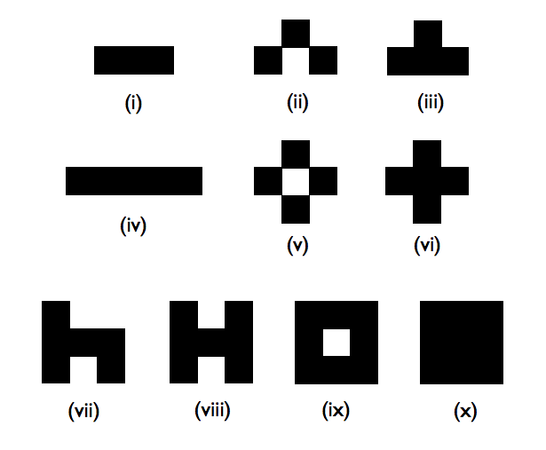
Figure 1: Some two-dimensional neighborhoods (Figs. (i) and (iv) are three and five cells wide, respectively).

2 Odd-rule CAs

We consider cellular automata whose cells form a $d$-dimensional cubic lattice $\mathbb{Z}^{d}$, where $d$ is 1, 2, or 3. Each cell is either ON or OFF, and an ON cell with center at the lattice point $u=(u_{1},u_{2},\ldots,u_{d})\in\mathbb{Z}^{d}$ will be identified with the monomial $x^{u}=x_{1}^{u_{1}}x_{2}^{u_{2}}\cdots x_{d}^{u_{d}}$, which we regard as an element of the ring of Laurent polynomials ${\cal{R}}=\operatorname{GF}(2)[x_{1},x_{1}^{-1},\ldots,x_{d},x_{d}^{-1}]$ with mod 2 coefficients. The state of the CA is specified by giving the formal sum $S$ of all its ON cells. As long as only finitely many cells are ON, $S$ is indeed a polynomial in the variables $x_{i}$ and $x_{i}^{-1}$, and is therefore an element of ${\cal{R}}$. We write $u\in S$ to indicate that $u$ is ON, i.e., that $x^{u}$ is a monomial in $S$.

In most of this paper we will focus on what may be called “odd-rule” CAs. An odd-rule CA is defined by specifying a neighborhood of the cell at the origin, given by an element $F\in{\cal{R}}$ listing the cells in the neighborhood. A typical example is the Moore neighborhood in $\mathbb{Z}^{2}$, which consists of the eight cells surrounding the cell at the origin in the square grid (see Fig. 1(ix)), and is specified by

$$F \leavevmode\nobreak\ :=\leavevmode\nobreak\ \frac{1}{xy}+\frac{1}{y}+\frac{x}{y}+\frac{1}{x}+x+\frac{y}{x}+y+xy$$

$$\leavevmode\nobreak\ =\leavevmode\nobreak\ \left(\frac{1}{x}+1+x\right)\left(\frac{1}{y}+1+y\right)-1\leavevmode\nobreak\ \in\leavevmode\nobreak\ {\cal{R}}=\operatorname{GF}(2)[x,x^{-1},y,y^{-1}].$$ (1)

The neighborhood of an arbitrary cell $u$ is obtained by shifting $F$ so it is centered at $u$, that is, by the product $x^{u}F\in{\cal{R}}$. Given $F$, the corresponding odd-rule CA is defined by the rule that the cell at $u$ is ON at generation $n+1$ if it is the neighbor of an odd number of cells that were ON at generation $n$, and is otherwise OFF.

Our goal is to find $a_{n}(F)$, the number of ON cells at the $n$th generation when the CA is started in generation 0 with a single ON cell at the origin. For odd-rule CAs there is a simple formula. The number of nonzero terms in an element $P\in{\cal{R}}$ will be denoted by $|P|$.

Theorem 1.

For an odd-rule CA with neighborhood $F$, the state at generation $n$ is equal to $F^{n}$, and $a_{n}(F)=|F^{n}|$.

Proof.

We use induction on $n$. By definition, the initial state is $1=F^{0}$, and $a_{0}(F)=1$. The ON cell at the origin turns ON all the cells in $F$, so the state at generation 1 is $F$ itself, and $a_{1}(F)=|F|$. Suppose the state at generation $n$ is $F^{n}$. An ON cell $w\in F^{n}$ will affect a cell $u$ if and only if $u$ is in the neighborhood of $w$, that is, if and only if $u\in wF$. For $u$ to be turned ON, there must be an odd number of cells $w\in F^{n}$ with $u\in wF$. Since the coefficients in ${\cal{R}}$ are evaluated mod 2, $u$ will be turned ON if and only if $u\in\sum_{w\in F^{n}}wF=F\sum_{w\in F^{n}}w=F.F^{n}=F^{n+1}$. So $F^{n+1}$ is precisely the state at generation $n+1$, and $a_{n+1}(F)=|F^{n+1}|$. ∎

3 The run length transform

We define an operation on number sequences, the “run length transform”. For an integer $n\geq 0$, let ${\cal{L}}(n)$ denote the list of the lengths of the maximal runs of 1s in the binary expansion of $n$. For example, since the binary expansion of 55 is 110111, containing runs of 1s of lengths 2 and 3, ${\cal{L}}(55)=[2,3]$. ${\cal{L}}(0)$ is the empty list, and ${\cal{L}}(n)$ for $n=1,\ldots,12$ is respectively $[1],[1],[2],[1],[1,1],[2],[3],[1],[1,1],[1,1],[1,2],[2]$ (A245562).

Definition. The run length transform of a sequence $[S_{n},n\geq 0]$ is the sequence $[T_{n},n\geq 0]$ given by

$$T_{n}\leavevmode\nobreak\ =\leavevmode\nobreak\ \prod_{i\in{\cal{L}}(n)}S_{i}.$$ (2)

Note that $T_{n}$ depends only on the lengths of the runs of 1s in the binary expansion of $n$, not on the order in which they appear. For example, since ${\cal{L}}(11)=[1,2]$ and ${\cal{L}}(13)=[2,1]$, $T_{11}=T_{13}=S_{1}S_{2}$. Also $T_{0}=1$ (the empty product), so the value of $S_{0}$ is never used, and will usually be taken to be 1. Further properties and additional examples of the run length transform will be given in §7. See especially Table 4, which shows how the transformed sequence has a natural division into blocks.

Define the height $\operatorname{ht}(P)$ of an element $P\in{\cal{R}}$ to be the maximal value of $|e_{i}|$ in any monomial $x_{1}^{e_{1}}\cdots x_{d}^{e_{d}}$ in $P$. If $\operatorname{ht}(P)=h$, the cells in $P$ are contained in a $d$-dimensional cube centered at the origin with edges that are $2h+1$ cells long. Note that $\operatorname{ht}(PQ)\leq\operatorname{ht}(P)+\operatorname{ht}(Q)$ and $\operatorname{ht}(P^{k})=k\operatorname{ht}(P)$.

The second property that makes odd-rule CAs easier to analyze than most is the following.

Theorem 2.

If $\operatorname{ht}(F)\leq 1$, then $[a_{n}(F),n\geq 0]$ is the run length transform of the subsequence

$$[a_{0}(F),a_{1}(F),a_{3}(F),a_{7}(F),a_{15}(F),\ldots,a_{2^{k}-1}(F),\ldots].$$ (3)

Proof.

The proof depends on the identity sometimes called the Freshman’s Dream, which in its simplest form states that $(x+y)^{2}\equiv x^{2}+y^{2}$ mod 2, and more generally that for $P(x_{1},x_{1}^{-1},\ldots)\in{\cal{R}}$,

$$P(x_{1},x_{1}^{-1},\ldots)^{2^{k}}\leavevmode\nobreak\ =\leavevmode\nobreak\ P(x_{1}^{2^{k}},x_{1}^{-2^{k}},\ldots),$$ (4)

for any integer $k\geq 0$, and in particular that $|P(x_{1},x_{1}^{-1},\ldots)^{2^{k}}|=|P|$. Suppose first that the binary expansion of $n$ contains exactly two runs of 1s, separated by one or more 0s, say

$$n\leavevmode\nobreak\ =\leavevmode\nobreak\ \overbrace{111\cdots 1}^{m_{1}}\overbrace{00\cdots 0}^{m_{2}}\overbrace{111\cdots 1}^{m_{3}},\quad m_{1},m_{2},m_{3}\geq 1,$$

i.e.,

$$n\leavevmode\nobreak\ =\leavevmode\nobreak\ (2^{m_{1}}-1)2^{m_{2}+m_{3}}+(2^{m_{3}}-1),$$

with ${\cal{L}}(n)=[m_{1},m_{3}]$. Then

$$F^{n}\leavevmode\nobreak\ =\leavevmode\nobreak\ (F^{2^{m_{1}}-1})^{2^{m_{2}+m_{3}}}F^{2^{m_{3}}-1}\leavevmode\nobreak\ =\leavevmode\nobreak\ P^{2^{m_{2}+m_{3}}}Q\mbox{\leavevmode\nobreak\ (say)},$$ (5)

where $P:=F^{2^{m_{1}}-1}$, $Q:=F^{2^{m_{3}}-1}$. Equation (5) states that $F^{n}$ is a sum of copies of $Q$ centered at the cells of of $P^{2^{m_{2}+m_{3}}}$. By the Freshman’s Dream, $P^{2^{m_{2}+m_{3}}}$ is a polynomial in the variables $x_{i}^{\pm 2^{m_{2}+m_{3}}}$, so the cells in $P^{2^{m_{2}+m_{3}}}$ are separated by at least $2^{m_{2}+m_{3}}$. Also, $|P^{2^{m_{2}+m_{3}}}|=|P|$. On the other hand, since $\operatorname{ht}(F)\leq 1$, $\operatorname{ht}(Q)\leq 2^{m_{3}}-1$, and since

$$2(2^{m_{3}}-1)+1\leavevmode\nobreak\ <\leavevmode\nobreak\ 2^{m_{3}+1}\leavevmode\nobreak\ \leq\leavevmode\nobreak\ 2^{m_{2}+m_{3}}$$

the copies of $Q$ in $F^{n}$ are disjoint from each other, and so $|F^{n}|=|P||Q|$, or in other words

$$a_{n}(F)\leavevmode\nobreak\ =\leavevmode\nobreak\ a_{2^{m_{1}}-1}(F)\leavevmode\nobreak\ a_{2^{m_{3}}-1}(F)\leavevmode\nobreak\ =\leavevmode\nobreak\ \prod_{i\in{\cal{L}}(n)}a_{2^{i}-1}(F).$$

It is straightforward to generalize this argument to the case when there are more than two runs of 1s in the binary expansion of $n$, and to establish that for any $n$,

$$a_{n}(F)\leavevmode\nobreak\ =\leavevmode\nobreak\ \prod_{i\in{\cal{L}}(n)}a_{2^{i}-1}(F),$$ (6)

thus completing the proof. ∎

In several interesting cases the subsequence (3) satisfies a three-term linear recurrence, in which case there is also a simple recurrence for the run length transform.

Theorem 3.

Suppose the sequence $[S_{n},n\geq 0]$ is defined by the recurrence $S_{n+1}=c_{2}S_{n}+c_{3}S_{n-1},n\geq 1$, with $S_{0}=1$, $S_{1}=c_{1}$. Then its run length transform $[T_{n},n\geq 0]$ satisfies the recurrence

$$T_{2t}=T_{t},\quad T_{4t+1}=c_{1}T_{t},\quad T_{4t+3}=c_{2}T_{2t+1}+c_{3}T_{t},$$ (7)

for $t>0$, with $T_{0}=1$.

Proof.

$T_{2t}=T_{t}$ is immediate from the definition of the run length transform, since ${\cal{L}}(2n)={\cal{L}}(n)$. The binary expansion of $4t+1$ ends in $01$, so $T_{4t+1}=T_{t}S_{1}=c_{1}T_{t}$. If $t=2^{k}-1$ for some $k\geq 1$ then $T_{4t+3}=S_{k+2}=c_{2}S_{k+1}+c_{3}S_{k}$, $T_{4t+1}=c_{1}S_{k}$, $T_{2t+1}=S_{k+1}$, implying

$$T_{4t+3}=c_{2}T_{2t+1}+c_{3}T_{t}.$$ (8)

On the other hand, if $t$ has a zero in its binary expansion, say $t=i.2^{k+1}+(2^{k}-1),k\geq 0$, then $T_{4t+3}=T_{i}S_{k+2}=T_{i}(c_{2}S_{k+1}+c_{3}S_{k})$, $T_{4t+1}=T_{i}c_{1}S_{k}$, $T_{2t+1}=T_{i}S_{k+1}$, and again (8) follows. ∎

4 Fredkin’s Replicator

The cellular automaton known as Fredkin’s Replicator [7, 8, 15] is the two-dimensional odd-rule CA defined by the Moore neighborhood $F$ shown in Fig. 1(ix) and Eq. (2). (This is the eight-neighbor totalistic Rule 52428 in the Wolfram numbering scheme [17, 24, 26].)

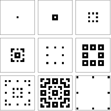
Figure 2: Generations 0 through 8 of the evolution of Fredkin’s Replicator. ON cells are black, OFF cells are white.

We study the evolution of this CA when it is started at generation 0 with a single ON cell at the origin. Generations 0 through 8 are shown in Fig. 2. The name of this CA comes from the fact that any configuration of ON cells will be replicated eight times at some later stage. For example, generation 1 is replicated eight times at generation 5. Although distinctive, the name is not especially appropriate, since by (4) any odd-rule CA has a similar replication property. Let $a_{n}(F)=a_{n}$ denote the number of ON cells at the $n$th generation. The initial values of $a_{n}$ are shown in Table 1.

Table 1: Number of ON cells at $n$th generation of Fredkin’s Replicator (A160239).

$$\begin{array}[]{c|rrrrrrrrrrrrrrrr}n&&&&&&&a_{n}\\ \hline\cr 0&\mathbf{1}\\ 1&\mathbf{8}\\ 2-3&8&\mathbf{24}\\ 4-7&8&64&24&\mathbf{112}\\ 8-15&8&64&64&192&24&192&112&\mathbf{416}\\ 16-31&8&64&64&192&64&512&192&896&24&192&192&576&112&896&416&\mathbf{1728}\\ 32-63&8&64&64&192&64&512&192&896&64&512&512&1536&\ldots\end{array}$$

Since $\operatorname{ht}(F)=1$, we know from Theorem 2 that $[a_{n},n\geq 0]$ is the run length transform of the subsequence $[b_{n}=a_{2^{n}-1},n\geq 0]=1,8,24,112,416,1728,\ldots$ (shown in bold in Table 1; it will turn out to be A246030). The main result of this section is the identification of this subsequence.

Theorem 4.

The sequence $[b_{n},n\geq 0]$ satisfies the recurrence

$$b_{n+1}\leavevmode\nobreak\ =\leavevmode\nobreak\ 2b_{n}+8b_{n-1},\leavevmode\nobreak\ {\mbox{w}ith\leavevmode\nobreak\ }b_{0}=1,b_{1}=8.$$ (9)

Proof.

Let $G_{n}:=F^{n}$, $H_{n}:=G_{2^{n}-1}=F^{2^{n}-1}$. (Figure 2 shows $G_{0}=H_{0}$, $G_{1}=H_{1}$, $G_{2}$, $G_{3}=H_{2}$, $G_{4}$, $G_{5}$, $G_{6}$, $G_{7}=H_{3}$, and $G_{8}$.) By definition,

$$H_{n+1}\leavevmode\nobreak\ =\leavevmode\nobreak\ F^{2^{n}}H_{n},$$ (10)

and, from Theorem 1, $a_{n}=|G_{n}|$, $b_{n}=|H_{n}|$.

Since $F$ has diameter 3, the nonzero terms $x^{i}y^{j}$ in $H_{n}$ satisfy

$$-(2^{n}-1)\leavevmode\nobreak\ \leq i,j\leq 2^{n}-1,$$ (11)

so we can write

$$H_{n}\leavevmode\nobreak\ =\leavevmode\nobreak\ \sum_{i=-(2^{n}-1)}^{2^{n}-1}\,\sum_{j=-(2^{n}-1)}^{2^{n}-1}H_{n}(i,j)x^{i}y^{j},$$ (12)

where the coefficient $H_{n}(i,j)\in\operatorname{GF}(2)$ gives the state of the cell $(i,j)$ at generation $n$.

From (10) and (4), $H_{n+1}$ is the sum (in ${\cal{R}}$) of eight copies of $H_{n}$, translated by $2^{n}$ in each of the N, NW, W, SW, S, SE, E, and NE directions. That is, for $n\geq 1$,

$$H_{n+1}(i,j) \leavevmode\nobreak\ =\leavevmode\nobreak\ H_{n}(i,j-2^{n})+H_{n}(i-2^{n},j-2^{n})+H_{n}(i-2^{n},j)+H_{n}(i-2^{n},j+2^{n})$$

$$\leavevmode\nobreak\ \leavevmode\nobreak\ +H_{n}(i,j+2^{n})+H_{n}(i+2^{n},j+2^{n})+H_{n}(i+2^{n},j)+H_{n}(i+2^{n},j-2^{n}),$$ (13)

where we adopt the convention that $H_{n}(i,j)=0$ unless $i$ and $j$ satisfy (11). Also,

$$H_{0}(0,0)=1,\leavevmode\nobreak\ \leavevmode\nobreak\ H_{0}(i,j)=0\mbox{\leavevmode\nobreak\ for\leavevmode\nobreak\ }(i,j)\neq(0,0),$$ (14)

and $H_{1}(i,j)=0$ except for

$$H_{1}(0,1) =H_{1}(-1,1)=H_{1}(-1,0)=H_{1}(-1,-1)$$

$$=H_{1}(0,-1)=H_{1}(1,-1)=H_{1}(1,0)=H_{1}(1,1)=1.$$ (15)

By construction, $H_{n}$ is preserved by the action of the dihedral group of order 8 (the symmetry group of the square), generated by the action of $(x,y)\leftrightarrow(y,x)$ and $(x,y)\leftrightarrow(\frac{1}{x},y)$. We study $H_{n}$ by breaking it up into the central cell, the four parts on the axes, and the four quadrants.

The central cell. The central cell $H_{n}(0,0)=1$ if $n=0$, and (as a consequence of the 8-fold symmetry) is 0 for $n>0$. The axial parts. We define $X_{n}$ ($n\geq 1$) to be the portion of $H_{n}$ that lies on the positive $x$-axis, but normalized so that its center is at the origin:

$$X_{n}\leavevmode\nobreak\ :=\leavevmode\nobreak\ \frac{1}{x^{2^{n-1}}}\,\sum_{i=1}^{2^{n}-1}H_{n}(i,0)x^{i}.$$ (16)

For example, $X_{1}=1,X_{2}=\frac{1}{x}+x,X_{3}=\frac{1}{x^{3}}+\frac{1}{x}+x+x^{3}$. From (4) it follows by induction that, for $n\geq 2$,

$$X_{n}\leavevmode\nobreak\ =\leavevmode\nobreak\ \sum_{i=0}^{2^{n-2}-1}\left(x^{-(2i+1)}+x^{2i+1}\right)\leavevmode\nobreak\ =\leavevmode\nobreak\ \left(\frac{1}{x}+x\right)^{2^{n-1}-1}.$$ (17)

Similarly, the portion of $H_{n}$ that lies on the negative $x$-axis, normalized so that its center is at the origin, is

$$\widetilde{X}_{n}\leavevmode\nobreak\ :=\leavevmode\nobreak\ x^{2^{n-1}}\,\sum_{i=1}^{2^{n}-1}H_{n}(-i,0)x^{-i}\leavevmode\nobreak\ =\leavevmode\nobreak\ \left(\frac{1}{x}+x\right)^{2^{n-1}-1}\leavevmode\nobreak\ =\leavevmode\nobreak\ X_{n}.$$ (18)

Likewise, the normalized portions of $H_{n}$ on the positive and negative $y$-axes are

$$Y_{n}\leavevmode\nobreak\ =\leavevmode\nobreak\ \widetilde{Y_{n}}\leavevmode\nobreak\ =\leavevmode\nobreak\ \left(\frac{1}{y}+y\right)^{2^{n-1}-1}.$$ (19)

The four quadrants. Next, define $\operatorname{I}_{n}$ for $n\geq 1$ to consist of the portion of $H_{n}$ lying in the first quadrant, again normalized so that its center is at the origin:

$$\operatorname{I}_{n}\leavevmode\nobreak\ :=\leavevmode\nobreak\ \frac{1}{(xy)^{2^{n-1}}}\,\sum_{i=1}^{2^{n}-1}\sum_{j=1}^{2^{n}-1}H_{n}(i,j)x^{i}y^{j}.$$ (20)

Similarly, we define

$$\operatorname{II}_{n} \leavevmode\nobreak\ :=\leavevmode\nobreak\ \left(\frac{x}{y}\right)^{2^{n-1}}\,\sum_{i=1}^{2^{n}-1}\sum_{j=1}^{2^{n}-1}H_{n}(-i,j)x^{-i}y^{j},$$

$$\operatorname{III}_{n} \leavevmode\nobreak\ :=\leavevmode\nobreak\ (xy)^{2^{n-1}}\,\sum_{i=1}^{2^{n}-1}\sum_{j=1}^{2^{n}-1}H_{n}(-i,-j)x^{-i}y^{-j},$$

$$\operatorname{IV}_{n} \leavevmode\nobreak\ :=\leavevmode\nobreak\ \left(\frac{y}{x}\right)^{2^{n-1}}\,\sum_{i=1}^{2^{n}-1}\sum_{j=1}^{2^{n}-1}H_{n}(i,-j)x^{i}y^{-j}.$$ (21)

Assembling the parts, we see that, for $n\geq 1$, $H_{n}=$

$$\begin{matrix}&\leavevmode\nobreak\ &(y/x)^{2^{n-1}}\operatorname{II}_{n}&+&y^{2^{n-1}}Y_{n}&+&(xy)^{2^{n-1}}\operatorname{I}_{n}\\ &+&(1/x)^{2^{n-1}}\leavevmode\nobreak\ \widetilde{X}_{n}&+&0&+&\leavevmode\nobreak\ \leavevmode\nobreak\ x^{2^{n-1}}\leavevmode\nobreak\ X_{n}\\ &+&(xy)^{-2^{n-1}}\operatorname{III}_{n}&+&y^{-2^{n-1}}\widetilde{Y}_{n}&+&(x/y)^{2^{n-1}}\operatorname{IV}_{n}\end{matrix}$$

which we write as a matrix

$$H_{n}\leavevmode\nobreak\ =\leavevmode\nobreak\ \begin{bmatrix}\operatorname{II}_{n}&Y_{n}&\operatorname{I}_{n}\\ \widetilde{X}_{n}&0&X_{n}\\ \operatorname{III}_{n}&\widetilde{Y}_{n}&\operatorname{IV}_{n}\end{bmatrix},$$ (22)

where it is to be understood that the blocks are to be shifted by the appropriate amounts (that is, the $\operatorname{I}_{n}$ in the top right corner is to be multiplied by $(xy)^{2^{n-1}}$, and so on). By summing the eight translated copies of $H_{n}$, as in (4), we obtain

$$H_{n+1}=\begin{bmatrix}\operatorname{II}_{n}&Y_{n}&\operatorname{I}_{n}+\operatorname{II}_{n}&Y_{n}&\operatorname{I}_{n}+\operatorname{II}_{n}&Y_{n}&\operatorname{I}_{n}\\ \widetilde{X}_{n}&0&X_{n}+\widetilde{X}_{n}&0&X_{n}+\widetilde{X}_{n}&0&X_{n}\\ \operatorname{II}_{n}+\operatorname{III}_{n}&Y_{n}+\widetilde{Y}_{n}&\operatorname{I}_{n}+\operatorname{III}_{n}+\operatorname{IV}_{n}&\widetilde{Y}_{n}&\operatorname{II}_{n}+\operatorname{III}_{n}+\operatorname{IV}_{n}&Y_{n}+\widetilde{Y}_{n}&\operatorname{I}_{n}+\operatorname{IV}_{n}\\ \widetilde{X}_{n}&0&X_{n}&0&\widetilde{X}_{n}&0&X_{n}\\ \operatorname{II}_{n}+\operatorname{III}_{n}&Y_{n}+\widetilde{Y}_{n}&\operatorname{I}_{n}+\operatorname{II}_{n}+\operatorname{IV}_{n}&Y_{n}&\operatorname{I}_{n}+\operatorname{II}_{n}+\operatorname{III}_{n}&Y_{n}+\widetilde{Y}_{n}&\operatorname{I}_{n}+\operatorname{IV}_{n}\\ \widetilde{X}_{n}&0&X_{n}+\widetilde{X}_{n}&0&X_{n}+\widetilde{X}_{n}&0&X_{n}\\ \operatorname{III}_{n}&\widetilde{Y}_{n}&\operatorname{III}_{n}+\operatorname{IV}_{n}&\widetilde{Y}_{n}&\operatorname{III}_{n}+\operatorname{IV}_{n}&\widetilde{Y}_{n}&\operatorname{IV}_{n}\end{bmatrix}.$$ (23)

Using (18) and (19), we have

$$\operatorname{II}_{n+1}=\begin{bmatrix}\operatorname{II}_{n}&Y_{n}&\operatorname{I}_{n}+\operatorname{II}_{n}\\ X_{n}&0&0\\ \operatorname{II}_{n}+\operatorname{III}_{n}&0&\operatorname{I}_{n}+\operatorname{III}_{n}+\operatorname{IV}_{n}\end{bmatrix},\leavevmode\nobreak\ \leavevmode\nobreak\ \operatorname{I}_{n+1}=\begin{bmatrix}\operatorname{I}_{n}+\operatorname{II}_{n}&Y_{n}&\operatorname{I}_{n}\\ 0&0&X_{n}\\ \operatorname{II}_{n}+\operatorname{III}_{n}+\operatorname{IV}_{n}&0&\operatorname{I}_{n}+\operatorname{IV}_{n}\end{bmatrix},$$ (24)

$$\operatorname{III}_{n+1}=\begin{bmatrix}\operatorname{II}_{n}+\operatorname{III}_{n}&0&\operatorname{I}_{n}+\operatorname{II}_{n}+\operatorname{IV}_{n}\\ X_{n}&0&0\\ \operatorname{III}_{n}&Y_{n}&\operatorname{III}_{n}+\operatorname{IV}_{n}\end{bmatrix},\leavevmode\nobreak\ \leavevmode\nobreak\ \operatorname{IV}_{n+1}=\begin{bmatrix}\operatorname{I}_{n}+\operatorname{II}_{n}+\operatorname{III}_{n}&0&\operatorname{I}_{n}+\operatorname{IV}_{n}\\ 0&0&X_{n}\\ \operatorname{III}_{n}+\operatorname{IV}_{n}&Y_{n}&\operatorname{IV}_{n}\end{bmatrix},$$ (25)

By adding these four matrices we find that $\operatorname{I}_{n+1}+\operatorname{II}_{n+1}+\operatorname{III}_{n+1}+\operatorname{IV}_{n+1}=0$ for $n\geq 1$. This identity is also true for $n=0$, and we conclude that

$$\operatorname{I}_{n}+\operatorname{II}_{n}+\operatorname{III}_{n}+\operatorname{IV}_{n}=0,\quad n\geq 1,$$ (26)

and so

$$\operatorname{II}_{n+1}=\begin{bmatrix}\operatorname{II}_{n}&Y_{n}&\operatorname{I}_{n}+\operatorname{II}_{n}\\ X_{n}&0&0\\ \operatorname{II}_{n}+\operatorname{III}_{n}&0&\operatorname{II}_{n}\end{bmatrix},\leavevmode\nobreak\ \leavevmode\nobreak\ \operatorname{I}_{n+1}=\begin{bmatrix}\operatorname{I}_{n}+\operatorname{II}_{n}&Y_{n}&\operatorname{I}_{n}\\ 0&0&X_{n}\\ \operatorname{I}_{n}&0&\operatorname{I}_{n}+\operatorname{IV}_{n}\end{bmatrix},\leavevmode\nobreak\ \leavevmode\nobreak\$$ (27)

etc., and finally that, for $n\geq 1$,

$$H_{n+1}=\begin{bmatrix}\operatorname{II}_{n}&Y_{n}&\operatorname{I}_{n}+\operatorname{II}_{n}&Y_{n}&\operatorname{I}_{n}+\operatorname{II}_{n}&Y_{n}&\operatorname{I}_{n}\\ X_{n}&0&0&0&0&0&X_{n}\\ \operatorname{II}_{n}+\operatorname{III}_{n}&0&\operatorname{II}_{n}&Y_{n}&\operatorname{I}_{n}&0&\operatorname{I}_{n}+\operatorname{IV}_{n}\\ X_{n}&0&X_{n}&0&X_{n}&0&X_{n}\\ \operatorname{II}_{n}+\operatorname{III}_{n}&0&\operatorname{III}_{n}&Y_{n}&\operatorname{IV}_{n}&0&\operatorname{I}_{n}+\operatorname{IV}_{n}\\ X_{n}&0&0&0&0&0&X_{n}\\ \operatorname{III}_{n}&Y_{n}&\operatorname{III}_{n}+\operatorname{IV}_{n}&Y_{n}&\operatorname{III}_{n}+\operatorname{IV}_{n}&Y_{n}&\operatorname{IV}_{n}\end{bmatrix}.$$ (28)

In (28) we see that $H_{n+1}$ contains a copy of $H_{n}$ at its center. The four corner blocks together with two copies each of $X_{n}$ and $Y_{n}$ form another, “deconstructed”, copy of $H_{n}$.

Suppose $n\geq 2$, and consider the blocks $[\operatorname{I}_{n}+\operatorname{II}_{n}\leavevmode\nobreak\ Y_{n}\leavevmode\nobreak\ \operatorname{I}_{n}+\operatorname{II}_{n}\leavevmode\nobreak\ Y_{n}]$ in the top row of (28). Using (27) these blocks can be expanded to give

$$\begin{bmatrix}\operatorname{I}_{n-1}&0&\operatorname{II}_{n-1}&Y_{n-1}&\operatorname{I}_{n-1}&0&\operatorname{II}_{n-1}&Y_{n-1}\\ X_{n-1}&0&X_{n-1}&0&X_{n-1}&0&X_{n-1}&0\\ \operatorname{IV}_{n-1}&0&\operatorname{III}_{n-1}&Y_{n-1}&\operatorname{IV}_{n-1}&0&\operatorname{III}_{n-1}&Y_{n-1}\end{bmatrix}.$$ (29)

The central three columns (columns 3, 4, and 5) give a copy of $H_{n-1}$, and columns 7, 8, and 1, in that order, give another copy. We get two further copies of $H_{n-1}$ from the analogous blocks in each of the other three sides of (28), so in total $H_{n+1}$ contains as many ON cells as are in two copies of $H_{n}$ plus eight copies of $H_{n-2}$. This implies (9) for $n\geq 2$. Equation (9) is certainly true for $n=1$, so this completes the proof of the theorem. ∎

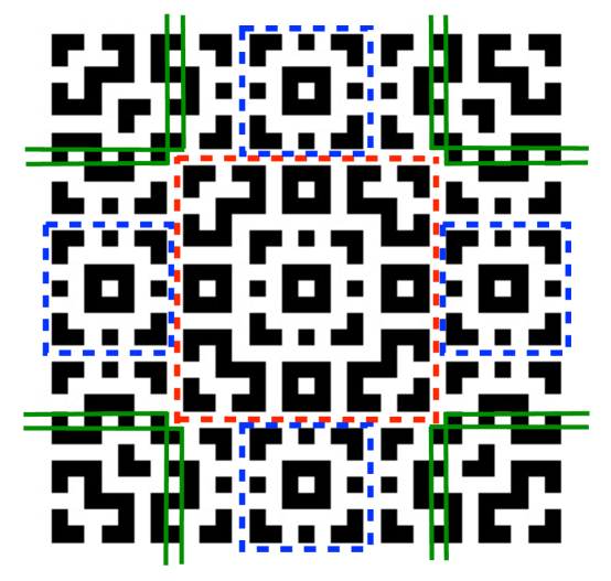
Figure 3: Dissection of $H_{4}$ into pieces that can be reassembled to give two copies of $H_{3}$ and eight copies of $H_{2}$, illustrating (9) in the case $n=3$.

The characteristic polynomial of (9) is $x^{2}-2x-8=(x+2)(x-4)$, and it follows that

$$b_{n}\leavevmode\nobreak\ =\leavevmode\nobreak\ \frac{5.4^{n}+(-2)^{n+1}}{3},\leavevmode\nobreak\ n\geq 0.$$ (30)

In geometric terms, the proof of Theorem 4 shows that $H_{n+1}$ can be dissected into pieces that can be reassembled to give two copies of $H_{n}$ and eight copies of $H_{n-1}$. Figure 3 shows this dissection in the case of $H_{4}$. The central dashed square (colored red in the online version) encloses a copy of $H_{3}$. The smaller dashed squares on the four sides (colored blue) enclose copies of $H_{2}$. The four pairs of vertical parallel lines (colored green) enclose copies of $Y_{3}$, and the four pairs of horizontal parallel lines (also green) enclose copies of $X_{3}$. The four corners (outside the parallel lines) are, reading counter-clockwise from the top right corner, respectively $\operatorname{I}_{3}$, $\operatorname{II}_{3}$, $\operatorname{III}_{3}$, and $\operatorname{IV}_{3}$, and combine with two copies each of $X_{3}$ and $Y_{3}$ to give the second copy of $H_{3}$. Along the top edge, the figure is divided into seven pieces, as in the top row of (28). By taking the fifth, sixth, and third pieces in that order gives another copy of $H_{2}$, and three further copies are obtained from the other edges of the figure.

From Theorem 3 and (9), we see that $a_{n}$ is given by the recurrence

$$a_{2t}=a_{t},\quad a_{4t+1}=8a_{t},\quad a_{4t+3}=2a_{2t+1}+8a_{t},$$ (31)

for $t>0$, with $a_{0}=1$, as conjectured by Hrothgar [10].

5 The centered von Neumann neighborhood

In this section we analyze the two-dimensional odd-rule CA defined by the five-celled neighborhood

$$F\leavevmode\nobreak\ =\leavevmode\nobreak\ \frac{1}{x}+1+x+\frac{1}{y}+y\leavevmode\nobreak\ \in\leavevmode\nobreak\ {\cal{R}}=\operatorname{GF}(2)[x,x^{-1},y,y^{-1}]$$ (32)

shown in Fig. 1(vi), and consisting of the von Neumann neighborhood together with its center. (This is the five-neighbor totalistic Rule 614.) We use the same notation as in the previous section, except that now $F$ is defined by (32) instead of (2).

The initial values of $[a_{n},n\geq 0]$ are

$$\mathbf{1},\mathbf{5},5,\mathbf{17},5,25,17,\mathbf{61},5,25,25,85,17,85,61,\mathbf{217},\ldots$$

(A072272), which we know from Theorem 2 is the run length transform of the subsequence $[b_{n},n\geq 0]=1,5,17,61,217,773,2753,\ldots$, shown in bold (A007483). Generations 0 through 8 are shown in Fig. 4, and Figs. 5 and 6 show generation 31.

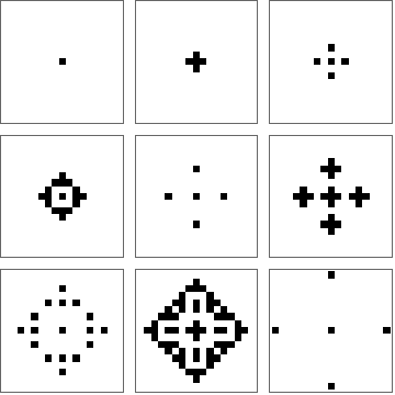
Figure 4: Generations 0 through 8 of the odd-rule CA defined by the centered von Neumann neighborhood. Generations 0, 1, 3, 7 show $H_{0}$, $H_{1}$, $H_{2}$, $H_{3}$ respectively.

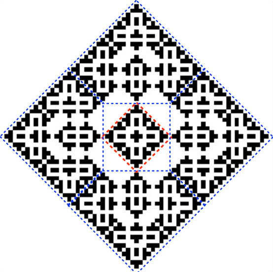
Figure 5: Generation 31 ($H_{5}$), showing dissection into central copy of $H_{3}$ (inside red dashed line) and four “haystacks” $N_{5}$, $W_{5}$, $S_{5}$, $E_{5}$ (each enclosed by blue dashed line).

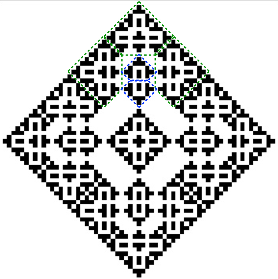
Figure 6: Another view of generation 31 ($H_{5}$) showing dissection of haystack $N_{5}$ into three smaller haystacks $N_{4}$, $W_{4}$, $E_{4}$ (each enclosed in green dashed line) and two still smaller haystacks $N_{3}$ and $S_{3}$ (inside blue dashed lines).

Theorem 5.

The sequence $[b_{n},n\geq 0]$ satisfies the recurrence

$$b_{n+1}\leavevmode\nobreak\ =\leavevmode\nobreak\ 3b_{n}+2b_{n-1},\leavevmode\nobreak\ \mbox{\leavevmode\nobreak\ with\leavevmode\nobreak\ }b_{0}=1,b_{1}=5.$$ (33)

Proof.

As in the proof of Theorem 4, $H_{n}=F^{2^{n}-1}$, $b_{n}=|H_{n}|$, and again $H_{n}$ is preserved under the action of a dihedral group of order 8. The first step in the proof is to show that for $n\geq 2$, $H_{n}$ can be dissected into a central copy of $H_{n-2}$ and four disjoint pentagonal or “haystack”-shaped regions (see Fig. 5 for the dissection of $H_{5}$). The four haystacks in $H_{n}$ will be denoted by $N_{n}$, $W_{n}$, $S_{n}$, and $E_{n}$, according to the direction in which they point (a precise definition will be given below). They are equivalent under the action of the dihedral group. Algebraically, we will show that

$$H_{n}\leavevmode\nobreak\ =\leavevmode\nobreak\ H_{n-2}+y^{2^{n-1}}N_{n}+x^{-2^{n-1}}W_{n}+y^{-2^{n-1}}S_{n}+x^{2^{n-1}}E_{n},$$ (34)

where the five polynomials on the right are disjoint (i.e., have no monomials in common with each other).

Once we have established (34), the second step in the proof will be to show that each haystack can be dissected into five smaller haystacks (see Fig. 6 for the dissection of $N_{5}$). In particular, we will show that for $n\geq 3$,

$$N_{n}\leavevmode\nobreak\ =\leavevmode\nobreak\ y^{2^{n-2}}N_{n-1}+x^{-2^{n-2}}W_{n-1}+x^{2^{n-2}}E_{n-1}+N_{n-2}+y^{-2^{n-3}}S_{n-2},$$ (35)

where again the polynomials on the right are disjoint. Let $\nu_{n}:=|N_{n}|=|W_{n}|=|S_{n}|=|E_{n}|$. Then (35) implies $\nu_{n}=3\nu_{n-1}+2\nu_{n-2}$. From (34) we have $b_{n}=b_{n-2}+4\nu_{n}$, so

$$b_{n+1}-3b_{n}-2b_{n-1}=b_{n-1}-3b_{n-2}-2b_{n-3}=\cdots=\mbox{\leavevmode\nobreak\ either\leavevmode\nobreak\ }b_{3}-3b_{2}-2b_{1}\mbox{\leavevmode\nobreak\ or\leavevmode\nobreak\ }b_{2}-3b_{1}-2b_{0},$$

and each of the last two expressions evaluates to zero. This will complete the proof of (33). It is worth remarking that these dissections are of a different nature from the dissection in the previous section. There it was necessary to make some non-obvious cuts through the contiguous blocks of ON cells, as shown by the parallel (green) lines in the corners of Fig. 3. In contrast, in the present proof, the dissections are carried out by “tearing” along the obvious “perforations”, rather like tearing apart a block of postage stamps.

Now to the details. It follows from the definition (see the sequence of successive states in Fig. 4) that $H_{n}$ is a diamond-shaped configuration with extreme points $(\pm(2^{n}-1),0)$, $(0,\pm(2^{n}-1))$. Also, for $n\geq 2$, $H_{n}$ contains a copy of $H_{n-2}$ at its center, surrounded by a layer, at least one cell wide, of OFF cells. This follows from the identity

$$H_{n}-H_{n-2}\leavevmode\nobreak\ =\leavevmode\nobreak\ F^{2^{n}-1}-F^{2^{n-2}-1}\leavevmode\nobreak\ =\leavevmode\nobreak\ H_{n-2}(1+H_{2}^{2^{n-2}}),$$

upon checking that the right-hand side contains no monomials $x^{i}y^{j}$ with $|i|+|j|\leq 2^{n-2}$. The buffer layer of OFF cells around the central $H_{n-2}$ consists of the cells $x^{i}y^{j}$ with $|i|+|j|=2^{n-2}$.

We define the $n$th North haystack to be

$$N_{n}\leavevmode\nobreak\ :=\leavevmode\nobreak\ H_{n-2}\,T_{N}^{2^{n-2}},\leavevmode\nobreak\ n\geq 2,$$ (36)

where $T_{N}:=1/x+1+x+y$ is the four-celled North-pointing triangle shown in Fig. 1(iii). Similarly, the West, South, and East haystacks are

$$W_{n}\leavevmode\nobreak\ :=\leavevmode\nobreak\ H_{n-2}\,T_{W}^{2^{n-2}},\leavevmode\nobreak\ S_{n}\leavevmode\nobreak\ :=\leavevmode\nobreak\ H_{n-2}\,T_{S}^{2^{n-2}},\leavevmode\nobreak\ E_{n}\leavevmode\nobreak\ :=\leavevmode\nobreak\ H_{n-2}\,T_{E}^{2^{n-2}},$$ (37)

where $T_{W}:=1/x+1/y+1+y$ is a West-pointing version of $T_{N}$, and similarly for $T_{S}$ and $T_{E}$. (The simple expressions in (36) and (37) were guessed by computing the actual haystacks in $H_{3}$ to $H_{6}$ and using Maple to factor them in ${\cal{R}}$.) The haystack $N_{n}$ has the property that all its cells are on or inside the convex hull of the five cells $x^{i}y^{j}$ with $(i,j)$ equal to

$$(0,2^{n-1}-1),(-2^{n-1}+1,0),(-2^{n-2},-2^{n-2}+1),(2^{n-2}-2^{n-2}+1),(-2^{n-1}+1,0).$$ (38)

To see this, consider what happens to $N_{n}$ one generation later: it becomes

$$FN_{n}\leavevmode\nobreak\ =\leavevmode\nobreak\ (FT_{N})^{2^{n-2}},$$ (39)

using the Freshman’s Dream (4), where $FT_{n}$ is the six-celled configuration

$$y^{2}+\frac{1}{x^{2}}+\frac{1}{xy}+\frac{1}{y}+\frac{x}{y}+x^{2}.$$

From (39), $FN_{n}$ is this configuration with the cells moved $2^{n-2}$ steps apart, and the cells (38) lie just inside it.

Note that the point $(0,0)$ is in the interior of $N_{n}$ at the intersection of the vertical line through the apex and the horizontal line joining the most Western and Eastern points. The powers of $x$ and $y$ in (34) and (35) are needed in order to translate the haystacks into their correct positions. Since we now know the boundaries of all the terms on the right side of (34), we can check that these five polynomials are indeed disjoint. We must still check that (34) is an identity. Using the Freshman’s Dream, this reduces to checking the identity

$$H_{2}\leavevmode\nobreak\ =\leavevmode\nobreak\ 1+y^{2}T_{N}+x^{-2}T_{W}+y^{-2}T_{S}+x^{2}T_{E},$$

which is true. This completes the proof that (34) is a proper dissection of $H_{n}$. The correctness of the dissection (35) is verified in a similar way; we omit the details. ∎

6 Other Cellular Automata

6.1 The 256 one-dimensional rules

There are 256 possible CAs based on the one-dimensional three-celled neighborhood shown in Fig. 1(i). These are the CAs labeled Rule 0 through Rule 255 in the Wolfram numbering scheme [17, 24, 26]. As usual we assume the automaton is started with a single ON cell, and let $a_{n}$ denote the number of ON cells after $n$ generations. Illustrations of the initial generations of all 256 CAs are shown on pages 54–56 of [26]. Many of these sequences were analyzed in [23]; see also [22]. If we eliminate those in which some $a_{n}$ is infinite, or the sequence $[a_{n},n\geq 0]$ is trivial (essentially linear), or is a duplicate of one of the others, we are left with just seven sequences:

• Rule 18 (or Rule 90; Rule 182 is very similar): $a_{n}=2^{\operatorname{wt}(n)}$ (Gould’s sequence A001316), where $\operatorname{wt}(n)$ is the number of 1s in the binary expansion of $n$. This is the run length transform of the powers of 2.

• Rule 22: $a_{n}=2^{\operatorname{wt}(n)}$ if $n$ even, $3.2^{\operatorname{wt}(n)-1}$ if $n$ odd (A071044).

• Rule 30: The behavior appears chaotic, even when started with a single ON cell [22, 26]. The sequence, A070952, has roughly linear growth, but it seems likely that there is no simpler way to obtain it than by its definition.

• Rule 62: $a_{n+7}=a_{n+4}+a_{n+3}-a_{n}$ with initial terms $1,3,3,6,5,8,9$ (A071047).

• Rule 110: Although the initial behavior is chaotic, it is an astonishing fact, pointed out by Wolfram [26, p. 39], that after about three thousand terms all the irregularities disappear. By using the Salvy-Zimmermann gfun package in Maple [18], we find that the sequence, A071049, satisfies a linear recurrence of order 469: for $n\geq 2854$,

  $$a_{n+469}\leavevmode\nobreak\ =\leavevmode\nobreak\ -a_{n+453}+a_{n+256}+a_{n+240}+a_{n+229}+a_{n+213}-a_{n+16}-a_{n}.$$ (40)

  This recurrence is far nicer than it initially appears: the coefficients are palindromic, and its characteristic polynomial is the product of 25 irreducible factors.

• Rule 126: $a_{n}=2^{\operatorname{wt}(n)+1}$, except we must subtract 1 if $n=2^{k}-1$ for some $k$ (A071051).

• Rule 150: This is the odd-rule CA defined by the three-celled neighborhood. The sequence $[a_{n},n\geq 0]$ (A071053) was analyzed by Wolfram [23] (see also [9], [19]). In the notation of the present paper $[a_{n},n\geq 0]$ is the run length transform of the Jacobstahl sequence A001045. Theorems 1 and 2 were suggested by reading Sillke’s analysis [19].

6.2 Other odd-rule CAs

In this section we discuss the odd-rule CAs defined by the height-one neighborhoods in Fig. 1. (The height-two neighborhood of Fig. 1(iv) is discussed in the last section of the paper.) Table 2 summarizes the results. The first column specifies the neighborhood $F$ in Fig. 1, $a_{n}(F)$ is the number of ON cells at generation $n$, $b_{n}(F)$ denotes the sequence of which $a_{n}(F)$ is the run length transform, and the fourth column gives a generating function (g.f.) for $b_{n}(f)$. For Fig. (iii), $\operatorname{Fib}_{n+2}$ denotes a Fibonacci number. The g.f. for (vii), found by Doron Zeilberger [3], is

$$\frac{\left(1+2\,x\right)\left(1+x-x^{2}+x^{3}+2\,{x}^{5}\right)}{1-3\,x-3\,{x}^{2}+{x}^{3}+6\,x^{4}-10\,x^{5}+8\,{x}^{6}-8\,{x}^{7}}\,.$$ (41)

An expanded version of this table, analyzing all the sequences arising from odd-rule CAs defined by height-one neighborhoods on the square grid, will be published elsewhere [4].

Table 2: Odd-rule CAs defined by height-1 neighborhoods $F$ in Fig. 1.

$$\begin{array}[]{|c|c|c|c|c|}\hline\cr F&a_{n}(F)&b_{n}(F)&\mbox{g.f.}&\mbox{Notes}\\ \hline\cr\mbox{(i)}&\href http://oeis.org/A071053&\href http://oeis.org/A001045&\frac{1+2x}{1-x-2x^{2}}&\mbox{Rule\leavevmode\nobreak\ 150},\leavevmode\nobreak\ \S\ref{Sec61}\\ \mbox{(ii)}&\href http://oeis.org/A048883&\href http://oeis.org/A000244&\frac{1}{1-3x}&a_{n}=3^{\operatorname{wt}(n)}\\ \mbox{(iii)}&\href http://oeis.org/A253064&\href http://oeis.org/A087206&\frac{1+2x}{1-2x-4x^{2}}&b_{n}=2^{n}\operatorname{Fib}_{n+2}\\ \mbox{(v)}&\href http://oeis.org/A102376&\href http://oeis.org/A000302&\frac{1}{1-4x}&a_{n}=4^{\operatorname{wt}(n)}\\ \mbox{(vi)}&\href http://oeis.org/A072272&\href http://oeis.org/A007483&\frac{1+2x}{1-3x-2x^{2}}&\S\ref{SecVN}\\ \mbox{(vii)}&\href http://oeis.org/A253069&\href http://oeis.org/A253070&(\ref{Eqviigf})&\\ \mbox{(viii)}&\href http://oeis.org/A246039&\href http://oeis.org/A246038&\frac{(1+2x)(1+2x+4x^{2})}{1-3x-8x^{3}-8x^{4}}&\\ \mbox{(ix)}&\href http://oeis.org/A160239&\href http://oeis.org/A246030&\frac{1+6x}{1-2x-8x^{2}}&\mbox{Fredkin\leavevmode\nobreak\ Replicator},\leavevmode\nobreak\ \S\ref{SecFR}\\ \mbox{(x)}&\href http://oeis.org/A246035&\href http://oeis.org/A139818&\frac{1+6x-8x^{2}}{(1-x)(1+2x)(1-4x)}&\mbox{Squares\leavevmode\nobreak\ of\leavevmode\nobreak\ entries\leavevmode\nobreak\ from\leavevmode\nobreak\ (i)}\\ \hline\cr\end{array}$$

6.3 Further two-dimensional CAs

If we drop the “odd-rule” definition, the number of CAs grows astronomically—there are $2^{512}$ based on the Moore neighborhood alone. Pages 171–175 of [26] show many examples of the subset of “totalistic” rules, in which the next state of a cell depends only on its present state and the total number of ON cells surrounding it. All of these are potential sources of sequences. In a few cases it is possible to analyze the sequence, but usually it seems that no formula or recurrence exists. In this section we give three examples: one that can be analyzed, one that might be analyzable with further research, and one (typical of the majority) where the state diagrams are aesthetically appealing but finding a formula seems hopeless. All three are totalistic rules, the first two being based on the von Neumann neighborhood (Fig. 1(v)), and the third on the Moore neighborhood (Fig. 1(ix)).

The first example is the Rule 750 automaton, in which an OFF cell turns ON if an odd number of its four neighbors are ON, and once a cell is ON it stays ON [26, p. 925]. This CA is a hybrid of the “odd-rule” CAs studied above and the “once a cell is ON it stays ON” rules studied in [2]. Here it is convenient to call the initial ON cell generation 1 (rather than 0). The numbers of ON cells in the first few generations (A169707) are given in Table 3.

Table 3: Number of ON cells at $n$th generation of CA defined by Rule 750.

$$\begin{array}[]{c|rrrrrrrrr}n&&&a_{n}\\ \hline\cr 1&1\\ 2-3&5&9\\ 4-7&21&25&37&57\\ 8-15&85&89&101&121&149&169&213&281\\ 16-31&341&345&357&377&405&425&469&\ldots\end{array}$$

The evolution of this CA is similar to several that were studied in [2]: at generation $2^{k}$, for $k\geq 2$, the structure is enclosed in a diamond-shaped region, which is saturated in the sense that no additional interior cells can ever be turned ON, and contains $a_{2^{k}}=(4^{k+1}-1)/3$ ON cells. Then in generations $2^{k}+1$ to $2^{k+1}-1$, the structure grows outwards from the four vertices of the diamond, and the first half of the growth that follows generation $2^{k}$ is the same as the the growth that followed generation $2^{k-1}$. Figure 7 shows generation $20=2^{4}+4$, where we can see that 16 cells have grown out of each vertex. Pictures of generations $16=2^{3}+4$ and $36=2^{5}+4$ show exactly the same growth from the vertices (although with different numbers of ON cells in the central diamond).

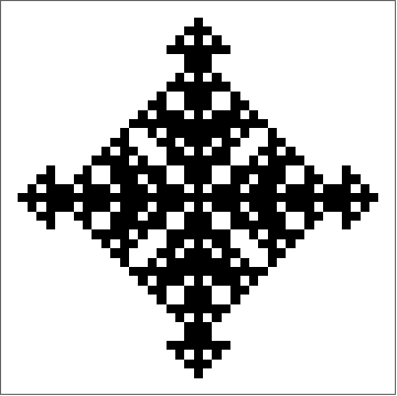
Figure 7: Generation 20 of CA defined by Rule 750, showing $341+4(1+3+5+7)=405$ ON cells, illustrating (43).

The successive numbers of ON cells added to a vertex in the generations from $2^{k}$ to $2^{k+1}-1$ are $0,1,3,5,7,5,11,17,15,5,\ldots$, which form the initial terms $v_{0},v_{1},v_{2},\ldots$ of a sequence (A151548) encountered in [2]. The $v_{i}$ have generating function

$$\frac{x}{1+x}\leavevmode\nobreak\ +\leavevmode\nobreak\ 4\,x^{2}\,\prod_{r=1}^{\infty}(1+x^{2^{r}-1}+2x^{2^{r}}).$$ (42)

Then, for $k\geq 0$ and $0\leq m<2^{k}$, we have

$$a_{2^{k}+m}\leavevmode\nobreak\ =\leavevmode\nobreak\ \frac{4^{k+1}-1}{3}\leavevmode\nobreak\ +\leavevmode\nobreak\ 4\sum_{i=0}^{m}v_{i}.$$ (43)

Bearing in mind the warning in the first sentence of this paper, we must admit that we have not written out a complete proof that (43) is correct. However, there should be no difficulty in filling in the details: as the automaton evolves from generation $2^{k}$ to $2^{k+1}$, the structure has a natural dissection into polygonal pieces.

The second example is more speculative: this is the Rule 493 automaton [26, p. 173], A246333. The binary expansions of 493 and 750 differ in just four places, so it is not surprising that this is similar to the previous example. Now an ON cell stays ON unless exactly zero or four of its neighbors are ON, in which case it turns OFF, and an OFF cell turns ON unless exactly two of its neighbors are ON. Assuming here that we start with a single ON cell at generation 0, in the even-numbered generations the number of ON cells is finite (A246334):

$$1,5,17,29,61,73,109,157,229,241,277,329,429,477,573,633,861,\ldots,$$

while in the odd-numbered generations the number of OFF cells is finite (A246335):

$$1,5,9,21,25,37,57,85,89,101,121,165,169,213,217,317,321,333,\ldots.$$

The reason for hoping this automaton might be analyzable is that the latter sequence agrees with the sequence in Table 3 up though the eleventh term, 121, after which the sequences diverge. Even the respective states are the same up through the sixth term, 37, although to see this one has to work with the negatives—in the photographer’s sense, interchanging black and while cells—and then rotating the result by 45 degrees. This needs further investigation.

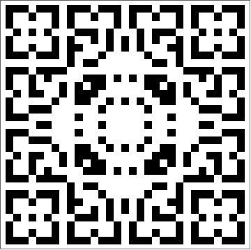
Figure 8: Generation 15 of CA defined by eight-neighbor Rule 780.

The third example in the eight-neighbor Rule 780 (A246310), in which a cell turns ON if one or four of its neighbors in ON, and otherwise turns OFF. Although the initial generations are simple enough, already by generation 15 (Fig. 8) the structure is extremely complicated. Is there a recurrence? Is the five-neighbor analog (A253086) any easier to understand?

6.4 The three-dimensional analog of Fredkin’s Replicator

The three-dimensional Moore neighborhood, that is, the $3\times 3\times 3$ cube without its center cell, gives rise to the sequence $1,26,26,124,26,676,124,1400,\ldots$ (A246031), which by Theorem 2 is the run length transform of the subsequence

$$1,26,124,1400,10000,89504,707008,5924480,47900416,393069824,3189761536,25963397888,\ldots$$ (44)

(A246032), computed by Roman Pearce and Michael Monagan. Doron Zeilberger [3] has found a generating function, a rational function with numerator of degree $10$ and denominator of degree $11$, as well as a proof that it is correct.

7 Further remarks about run length transforms

Block structure. It is a surprising fact that the growth sequences of many CAs have a natural division into blocks of successive lengths $(1,)1,2,4,8,16,32,\ldots$. This is true even for some CAs that are defined on lattices other than $\mathbb{Z}^{d}$ [2]. Some of these examples are explained by the fact that the run length transform always has this property—the division into blocks of the run length transform $[T_{n},n\geq 0]$ of an arbitrary sequence $S=[1,A,B,C,D,\ldots]$ is shown in Table 4. Table 1 above gives a concrete example. The first half of each row is given by $A$ times the beginning of the $[T_{n}]$ sequence itself.

Table 4: The run length transform $[T_{n},n\geq 0]$ of a sequence $S=[1,A,B,C,D,\ldots]$, showing the division into blocks of sizes $1,1,2,4,8,16,\ldots$.

$$\begin{array}[]{c|rrrrrrrrrrrrrrrr}n&&&&&&&T_{n}\\ \hline\cr 0&1\\ 1&A\\ 2-3&A&B\\ 4-7&A&A^{2}&B&C\\ 8-15&A&A^{2}&A^{2}&AB&B&AB&C&D\\ 16-31&A&A^{2}&A^{2}&AB&A^{2}&A^{3}&AB&AC&B&AB&AB&B^{2}&C&AC&D&E\\ 32-63&A&A^{2}&A^{2}&AB&A^{2}&A^{3}&AB&AC&\ldots&&&&\end{array}$$

Further examples. We briefly mention four additional examples of run length transforms. The run length transform of $0,1,2,3,4,\ldots$ is $1,1,1,2,1,1,2,3,1,\ldots$ (A227349), which gives the product of the lengths of runs of 1s in the binary representation of $n$. The primes, prefixed by 1, give $1,2,2,3,2,4,3,5,2,\ldots$ (A246029). The squares give $1,1,1,4,1,1,4,9,\ldots$ (A246595). The powers of 2 give $1,2,2,4,2,4,4,8,2,\ldots$, $2^{\operatorname{wt}(n)}$ (A001316, already mentioned in §6.1).

Graphs. The graphs of run length transforms are usually highly irregular, as one expects from Table 4. The partial sums of these sequences are naturally smoother, and generally have a family resemblance, with a bumpy appearance somewhat similar to what is seen in the Tagaki curve [1], [12]. The partial sums of the four examples in the previous paragraph are A253083, A253081, A253082, A006046, respectively, and the partial sums of the sequences arising from Fredkin’s Replicator, the sequence in Sect. 5, and the Rule 150 sequence in Sect. 6 are respectively A245542, A253908, A134659. The latter sequence is discussed in [6], and it would be interesting to see if the methods of that paper can be applied to the other six sequences. Also, is there any direct connection between the limiting form of these graphs for large $n$ and the Tagaki curve?

The generalized run length transform. There are analogs of Theorem 2 which apply to larger neighborhoods, although they are more complicated and not as useful. The following is a version which applies when the neighborhood $F$ has height at most 2. Whereas in Theorem 2, $a_{n}(F)$ was expressed as a product of terms from the subsequence $a_{m}(F)$ where the binary expansion of $m$ contained no zeros, now we need the values $a_{m}(F)$ where $m$ is any number whose binary expansion begins and ends with 1 and does not contain any pair of adjacent zeros. These are the numbers (A247648)

$$1,3,5,7,11,13,15,21,23,27,29,31,43,45,47,53,55,59,61,63,\ldots.$$ (45)

Suppose for simplicity that the binary expansion of $n$ has the form

$$n\leavevmode\nobreak\ =\leavevmode\nobreak\ \overbrace{\ast\ast\cdots\ast}^{m_{1}}\overbrace{00\cdots 0}^{m_{2}}\overbrace{\ast\ast\cdots\ast}^{m_{3}},\quad m_{1},m_{3}\geq 1,m_{2}\geq 2,$$

where the asterisks indicate strings of 0s and 1s that begin and end with 1s and do not contain any pair of adjacent zeros. If the first such string represents $N_{1}$ and the second $N_{2}$, then $a_{n}(F)=a_{N_{1}}(F)a_{N_{2}}(F)$. There is an analogous expression in the general case, expressing $a_{n}(F)$ as a product of terms $a_{m}(F)$ where $m$ belongs to (45).

To illustrate, suppose $F$ is the five-celled one-dimensional neighborhood shown in Fig. 1(iv), with height 2. The initial values of $a_{n}(F)$ are given in Table 5, with $a_{m}(F)$ for $m$ in (45) shown in bold. For example, the binary expansion of 167 is 10100111, so the generalized run length transform tells us that $a_{167}(F)=a_{5}(F)a_{7}(F)=17.19=323$. It follows from the generalized run length transform property that in each row of the table, the first one-eighth of the terms coincide with 5 times the beginning of the sequence itself.

Table 5: Number of ON cells at $n$th generation of of odd-rule one-dimensional CA defined by a 5-celled neighborhood (A247649).

$$\begin{array}[]{c|rrrrrrrrr}n&&&a_{n}\\ \hline\cr 0&\mathbf{1}\\ 1&\mathbf{5}\\ 2-3&5&\mathbf{7}\\ 4-7&5&\mathbf{17}&7&\mathbf{19}\\ 8-15&5&25&17&\mathbf{19}&7&\mathbf{31}&19&\mathbf{25}\\ 16-31&5&25&25&35&17&\mathbf{61}&19&\mathbf{71}&\ldots\end{array}$$

The bold-faced entries in Table 5 form A253085, and we end with one last question: is there an independent characterization of this sequence? An affirmative answer might make the generalized run length transform a lot more interesting. Much remains to be done in this subject!

Postscript, March 2015

After seeing an initial version of this paper, Doron Zeilberger observed that it is possible to use Theorems 1 and 2 to automate calculation of sequences giving the number of ON cells in odd-rule CAs, and in the case of height-one neighborhoods, to find and rigorously prove the correctness of generating functions for the sequences of which they are the run length transforms. Details will appear elsewhere [3, 4].

References

- [1] P. C. Allaart and K. Kawamura, The Takagi function: a survey, Real Analysis Exchange, 37 (2011/12), 1 -54; http://arxiv.org/abs/1110.1691.
- [2] D. Applegate, O. E. Pol, and N. J. A. Sloane, The toothpick sequence and other sequences from cellular automata, Congress. Numerant., 206 (2010), 157–191; http://arxiv.org/abs/1004.3036.
- [3] S. B. Ekhad, N. J. A. Sloane, and D. Zeilberger, A meta-algorithm for creating fast algorithms for counting ON cells in odd-rule cellular automata, Preprint, March 2015.
- [4] S. B. Ekhad, N. J. A. Sloane, and D. Zeilberger, “Odd-rule” cellular automata on the square grid, Preprint, March 2015.
- [5] D. Eppstein, Growth and decay in Life-like cellular automata, 2009; http://arxiv.org/abs/0911.2890.
- [6] S. Finch, P. Sebah, and Z.-Q. Bai, Odd entries in Pascal’s trinomial triangle, 2008; http://arxiv.org/abs/0802.2654.
- [7] E. Fredkin, Digital mechanics, an informational process based on reversible universal cellular automata, in Cellular Automata, Theory and Experiment, ed. H. Gutowitz, MIT Press, 1990, pp. 254–270.
- [8] E. Fredkin, Digital Mechanics (Working Draft), 2000; http://64.78.31.152/wp-content/uploads/2012/08/digital_mechanics_book.pdf.
- [9] H. Havermann et al., Entry A071053 in [16], 2002–present.
- [10] Hrothgar, Notes on a replicating automaton, Preprint, July 2014.
- [11] J. Kari, Theory of cellular automata: a survey, Theoret. Comput. Sci., 334 (2005), 3- 33.
- [12] J. C. Lagarias, The Takagi function and its properties, in Functions in Number Theory and Their Probabilistic Aspects, ed. K. Matsumoto et al., RIMS Lecture Notes, vol. B34, Res. Inst. Math. Sci., Kyoto, 2012, pp. 153–189; http://arxiv.org/abs/1112.4205.
- [13] J. Layman et al., Entry A160239 in [16], 2009–present.
- [14] O. Martin, A. M. Odlyzko, and S. Wolfram, Algebraic properties of cellular automata, Comm. Math. Phys., 93 (1984), 219–258.
- [15] S. Mitra and S. Kumar, Fractal replication in time-manipulated one-dimensional cellular automata, Complex Systems, 16 (2006), 191–207.
- [16] The OEIS Foundation Inc., The On-Line Encyclopedia of Integer Sequences, 1996–present; https://oeis.org.
- [17] N. H. Packard and S. Wolfram, Two-dimensional cellular automata, J. Statist. Phys., 38 (1985), 901–946.
- [18] B. Salvy and P. Zimmermann, GFUN: a Maple package for the manipulation of generating and holonomic functions in one variable, ACM Transactions on Mathematical Software, 20 (1994), 163–177.
- [19] T. Sillke, Odd trinomials: , 2004; http://www.mathematik.uni-bielefeld.de/~sillke/PUZZLES/trinomials.
- [20] D. Singmaster, On the cellular automaton of Ulam and Warburton, M500 Magazine of the Open University, No. 195 (December 2003), pp. 2–7; https://oeis.org/A079314/a079314.pdf.
- [21] S. M. Ulam, On some mathematical problems connected with patterns of growth of figures, in Mathematical Problems in the Biological Sciences, ed. R. E. Bellman, Proc. Sympos. Applied Math., Vol. 14, Amer. Math. Soc., 1962, pp. 215–224.
- [22] E. W. Weisstein, MathWorld, Entries for Rules 30, 90, 110, 150, 182, etc.; http://mathworld.wolfram.com/, 2004–present.
- [23] S. Wolfram, Statistical mechanics of cellular automata, Rev. Mod. Phys., 55 (1983), 601–644.
- [24] S. Wolfram, Universality and complexity in cellular automata (Cellular Automata, Los Alamos, 1983), Physica D, 10 (1984, 1 -35.
- [25] S. Wolfram, The Mathematica Book, Cambridge University Press and Wolfram Research, Inc., NY, 2000.
- [26] S. Wolfram, A New Kind of Science, Wolfram Media, Champaign, IL, 2002.
2010 Mathematics Subject Classification: Primary 11B85, 37B15.
Keywords: Automata sequences, cellular automata, Moore neighborhood, von Neumann neighborhood, odd-rule cellular automata, run length transform, Fredkin Replicator, Rule 110, Rule 150