Time Averaged Consensus in a Direct Coupled Coherent Quantum Observer Network for a Single Qubit Finite Level Quantum System

Abstract

This paper considers the problem of constructing a direct coupled quantum observer network for a single qubit quantum system. The proposed observer consists of a network of quantum harmonic oscillators and it is shown that the observer network output converges to a consensus in a time averaged sense in which each component of the observer estimates a specified output of the quantum plant. An example and simulations are included.

I Introduction

There has been significant interest in controlling multi-agent systems to achieve a consensus; e.g., see [1, 2]. Also, the problem of consensus in multi-agent estimation problems has been considered; e.g., see [3]. In addition, consensus has been considered in quantum multi-agent systems; see [4, 5]. The papers [6, 7] considered the problem of constructing a direct coupling quantum observer for a given quantum system. The problem of constructing an observer for a linear quantum system has been considered for example in [8]. The theory of linear quantum systems has been of considerable interest in recent years; e.g., see [9, 10]. For such system models, an important class of control problems are coherent quantum feedback control problems; e.g., see [9, 11]. In these control problems, both the plant and the controller are quantum systems and the controller is designed to optimize some performance index. The coherent quantum observer problem can be regarded as a special case of the coherent quantum feedback control problem in which the objective of the observer is to estimate the system variables of the quantum plant. The papers [6, 7] considered a direct coupling coherent observer problem in which the observer is directly coupled to the plant and not coupled via a field as in previous papers. This leads the papers [6, 7] to consider a notion of time-averaged convergence for the observers.

We extend the results of [7] to consider a direct coupled quantum observer for a single qubit quantum plant, which is a network of quantum harmonic oscillators. This quantum network is constructed so that each output converges to the plant output of interest in a time averaged sense. This is a form of time averaged quantum consensus.

II Quantum Systems

Quantum Plant

We first consider the dynamics of a single qubit spin system which will correspond to the quantum plant; see also [12]. The quantum mechanical behavior of the system is described in terms of the system observables which are self-adjoint operators on the complex Hilbert space $\mathfrak{H}_{p}={\mathbb{C}}^{2}$. The commutator of two scalar operators $x$ and $y$ in ${\mathfrak{H}_{p}}$ is defined as $[x,y]=xy-yx$. Also, for a vector of operators $x$ in ${\mathfrak{H}}_{p}$, the commutator of ${x}$ and a scalar operator $y$ in ${\mathfrak{H}_{p}}$ is the vector of operators $[{x},y]={x}y-y{x}$.

The vector of system variables for the single qubit spin system under consideration is

$$x_{p}=(x_{1},x_{2},x_{3})^{T}\triangleq(\sigma_{1},\sigma_{2},\sigma_{3}),$$

where $\sigma_{1}$, $\sigma_{2}$ and $\sigma_{3}$ are spin operators. Here, $x_{p}$ a vector of self-adjoint operators, i.e., $x_{p}=x_{p}^{\#}$. In particular $x_{p}(0)$ is represented by the Pauli matrices; i.e.,

$$\sigma_{1}(0) = \left(\begin{array}[]{cc}0&1\\ 1&0\end{array}\right),\;\;\sigma_{2}(0)=\left(\begin{array}[]{cc}0&-{\boldsymbol{i}}\\ {\boldsymbol{i}}&0\end{array}\right),$$

$$\sigma_{3}(0) = \left(\begin{array}[]{cc}1&0\\ 0&-1\end{array}\right).$$

The commutation relations for the spin operators are

$$[\sigma_{i},\sigma_{j}]=2{\boldsymbol{i}}\sum_{k}\epsilon_{ijk}\sigma_{k},$$ (3)

where $\epsilon_{ijk}$ denotes the Levi-Civita tensor. The dynamics of the system variables $x$ are determined by the system Hamiltonian which is a self-adjoint operator on $\mathfrak{H}_{p}$. The Hamiltonian is chosen to be linear in $x_{p}$; i.e.,

$${\mathcal{H}}_{p}=r_{p}^{T}x_{p}(0)\;\;$$

where $r_{p}\in{\mathbb{R}}^{3}$. The plant model is then given by the differential equation

$$\dot{x}_{p}(t) = -{\boldsymbol{i}}[x_{p}(t),\mathcal{H}_{p}];$$

$$= A_{p}x_{p}(t);\quad x_{p}(0)=x_{0p};$$

$$z_{p}(t) = C_{p}x_{p}(t)$$ (4)

where $z_{p}$ denotes the system variable to be estimated by the observer and $C_{p}\in\mathbb{R}^{1\times 3}$; e.g., see [12]. Also, $A_{p}\in{\mathbb{R}}^{3\times 3}$. In order to obtain an expression for the matrix $A_{p}$ in terms of $r_{p}$, we define the linear mapping $\Theta_{p}:{\mathbb{C}}^{3}\rightarrow{\mathbb{C}}^{3\times 3}$ as

$$\Theta_{p}(\beta)=\left(\begin{array}[]{ccc}0&\beta_{3}&-\beta_{2}\\ -\beta_{3}&0&\beta_{1}\\ \beta_{2}&-\beta_{1}&0\end{array}\right).$$ (5)

Then, it was shown in [12] that

$$-{\boldsymbol{i}}[x_{p}(t),r_{p}^{T}x_{p}(t)]=-2\Theta_{p}(r_{p})x_{p}(t)$$ (6)

and hence $A_{p}=-2\Theta_{p}(r_{p})$.

In addition, it is shown in [12] that the mapping $\Theta_{p}(\cdot)$ has the following properties:

$$\Theta_{p}(\beta)\gamma = -\Theta_{p}(\gamma)\beta,$$ (7)

$$\Theta_{p}(\beta)\beta = 0,$$ (8)

$$\Theta_{p}(\beta)\Theta_{p}(\gamma) = \gamma\beta^{T}-\beta^{T}\gamma I,$$ (9)

$$\Theta\left(\Theta_{p}(\beta)\gamma\right) = \Theta_{p}(\beta)\Theta_{p}(\gamma)-\Theta_{p}(\gamma)\Theta_{p}(\beta).$$ (10)

Quantum Observer Network The quantum observer network will be a linear quantum system of the form

$$\dot{x}(t) = Ax(t);\quad x(0)=x_{0}$$ (11)

where $A$ is a real matrix in $\mathbb{R}^{n\times n}$, and $x(t)=[\begin{array}[]{ccc}x_{1}(t)&\ldots&x_{n}(t)\end{array}]^{T}$ is a vector of system observables which are self-adjoint operators on an infinite dimensional Hilbert space $\mathfrak{H}$; e.g., see [9]. Here $n$ is assumed to be an even number and $\frac{n}{2}$ is the number of modes in the quantum system.

The initial system variables $x(0)=x_{0}$ are assumed to satisfy the commutation relations

$$[x_{j}(0),x_{k}(0)]=2i\Theta_{jk},\ \ j,k=1,\ldots,n,$$ (12)

where $\Theta_{o}$ is a real skew-symmetric matrix with components $\Theta_{jk}$. The matrix $\Theta_{o}$ is assumed to be of the form

$$\Theta_{o}={\rm diag}(J,J,\ldots,J)$$ (13)

where $J$ denotes the real skew-symmetric $2\times 2$ matrix

$$J=\left[\begin{array}[]{cc}0&1\\ -1&0\end{array}\right].$$

The system dynamics (11) are determined by the system Hamiltonian which is a self-adjoint operator on the underlying Hilbert space $\mathfrak{H}$. For the linear quantum systems under consideration, the system Hamiltonian will be a quadratic form $\mathcal{H}=\frac{1}{2}x(0)^{T}Rx(0)$, where $R$ is a real symmetric matrix. Then, the corresponding matrix $A$ in (11) is given by

$$A=2\Theta_{o}R.$$ (14)

where $\Theta_{o}$ is defined as in (13). e.g., see [9]. In this case, the system is said to be physically realizable and the commutation relations hold for all times greater than zero:

$$[x_{o}(t),x_{o}(t)^{T}] = x_{o}(t)x_{o}(t)^{T}-\left(x_{o}(t)x_{o}(t)^{T}\right)^{T}$$ (15)

$$= 2{\boldsymbol{i}}\Theta_{o}\ \mbox{for all }t\geq 0.$$

Remark 1

Note that that the Hamiltonian $\mathcal{H}$ is preserved in time for the system (11). Indeed, $\mathcal{\dot{H}}=\frac{1}{2}\dot{x}^{T}Rx+\frac{1}{2}x^{T}R\dot{x}=-x^{T}R\Theta_{o}Rx+x^{T}R\Theta_{o}Rx=0$ since $R$ is symmetric and $\Theta_{o}$ is skew-symmetric.

We now describe the linear quantum system of the form (11) which will correspond to the quantum observer network; see also [9, 13, 14]. This system is described by a non-commutative differential equation of the form

$$\dot{x}_{o}(t) = A_{o}x_{o}(t);\quad x_{o}(0)=x_{0o};$$

$$z_{o}(t) = C_{o}x_{o}(t)$$ (16)

where the observer output $z_{o}(t)$ is the observer network estimate vector and $A_{p}\in\mathbb{R}^{n_{o}\times n_{o}}$, $C_{o}\in\mathbb{R}^{\frac{n_{o}}{2}\times n_{o}}$. Also, $x_{o}(t)$ is the vector of self-adjoint non-commutative system variables; e.g., see [9]. We assume the observer network order $n_{o}$ is an even number with $N=\frac{n_{o}}{2}$ being the number of elements in the quantum observer network. We also assume that the plant variables commute with the observer variables. The system dynamics (16) are determined by the observer system Hamiltonian which is a self-adjoint operator on the underlying Hilbert space for the observer. For the quantum observer network under consideration, this Hamiltonian is given by a quadratic form: $\mathcal{H}_{o}=\frac{1}{2}x_{o}(0)^{T}R_{o}x_{o}(0)$, where $R_{o}$ is a real symmetric matrix. Then, the corresponding matrix $A_{o}$ in (16) is given by

$$A_{o}=2\Theta_{o}R_{o}$$ (17)

where $\Theta_{o}$ is defined as in (13). Furthermore, we will assume that the quantum observer network has a graph structure and is coupled to the quantum plant as illustrated in Figure 1.

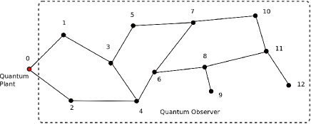
Figure 1: The graph $(\mathcal{G},E)$ for a typical quantum observer network.

The combined plant observer system is described by a connected graph $(\mathcal{G},E)$ which has $N+1$ nodes with node $0$ corresponding to the quantum plant and the remaining nodes, labelled $1,2,\ldots,N$, corresponding to the observer elements. This corresponds to an observer Hamiltonian of the form

$$\mathcal{H}_{o} = \frac{1}{2}x_{o}(0)^{T}R_{o}x_{o}(0)$$

$$= \frac{1}{2}\sum_{i=1}^{N}x_{oi}(0)^{T}R_{oi}x_{oi}(0)$$

$$+\frac{1}{2}\sum_{i=1}^{N}\sum_{j=1}^{N}x_{oi}(0)^{T}R_{cij}x_{oj}(0)$$

where the vector of observer system variables $x_{o}$ is partitioned according to each element of the quantum observer network as follows

$$x_{o}=\left[\begin{array}[]{l}x_{o1}\\ x_{o2}\\ \vdots\\ x_{oN}\end{array}\right].$$

We assume that the variables for each element of the quantum observer network commute with the variables of all other elements of the quantum observer network; i.e.,

$$[x_{oi},x_{oj}^{T}]=0~{}~{}\forall~{}~{}i\neq j.$$

Here, $x_{oi}=\left[\begin{array}[]{l}q_{oi}\\ p_{oi}\end{array}\right]$ for $i=1,2,\ldots,N$ where $q_{oi}$ is the position operator for the $i$th observer element and $p_{oi}$ is the momentum operator for the $i$th observer element.

In addition, we define a coupling Hamiltonian which defines the coupling between the quantum plant and the quantum observer network:

$$\mathcal{H}_{c}=\sum_{i=1}^{N}x_{p}(0)^{T}R_{c0i}x_{oi}(0).$$

Furthermore, we write

$$z_{o}=\left[\begin{array}[]{l}z_{o1}\\ z_{o2}\\ \vdots\\ z_{oN}\end{array}\right]$$

where

$$z_{oi}=C_{oi}x_{oi}\mbox{ for }i=1,2,\ldots,N.$$

Then

$$C_{o}=\left[\begin{array}[]{llll}C_{o1}&&&\\ &C_{o2}&0&\\ &0&\ddots&\\ &&&C_{oN}\end{array}\right].$$

Note that $R_{oi}\in\mathbb{R}^{2\times 2}$, $R_{cij}\in\mathbb{R}^{2\times 2}$, $C_{oi}\in\mathbb{R}^{1\times 2}$, and each matrix $R_{oi}$ is symmetric for $i=1,2,\ldots,N$, $j=1,2,\ldots,N$. In addition, $R_{c0j}\in\mathbb{R}^{3\times 2}$ for $j=1,2,\ldots,N$. Also, the matrices $R_{cij}$ for $i=0,1,\ldots,N$, $j=1,2,\ldots,N$ are such that $R_{cij}\neq 0$ if and only if $(i,j)\in E$, the set of edges for the graph $(\mathcal{G},E)$.

The augmented quantum linear system consisting of the quantum plant and the quantum observer network is described by the total Hamiltonian

$$\mathcal{H}_{a} = \mathcal{H}_{p}+\mathcal{H}_{c}+\mathcal{H}_{o}$$ (18)

$$= r_{p}^{T}x_{p}(0)+\frac{1}{2}\sum_{i=1}^{N}x_{oi}(0)^{T}R_{oi}x_{oi}(0)$$

$$+\frac{1}{2}\sum_{i=1}^{N}\sum_{j=1}^{N}x_{oi}(0)^{T}R_{cij}x_{oj}(0)$$

$$+\sum_{i=1}^{N}x_{p}(0)^{T}R_{c0i}x_{oi}(0).$$

Then, it follows that the augmented quantum system is described by the equations

$$\dot{x}_{p}(t) = -{\boldsymbol{i}}[x_{p}(t),\mathcal{H}_{a}];~{}x_{p}(0)=x_{0p};$$

$$\dot{x}_{o}(t) = -{\boldsymbol{i}}[x_{o}(t),\mathcal{H}_{a}];~{}x_{o}(0)=x_{0o};$$

$$z_{p}(t) = C_{p}x_{p}(t);$$

$$z_{o}(t) = C_{o}x_{o}(t);$$ (19)

e.g., see [12].

We now formally define the notion of a direct coupled linear quantum observer network.

Definition 1

The matrices $R_{oj}$, $R_{cij}$, $C_{oj}$ for $i=0,1,\ldots,N$, $j=1,2,\ldots,N$ and the graph $(\mathcal{G},E)$ define a linear quantum observer network achieving time-averaged consensus convergence for the single qubit quantum plant (4) if the corresponding augmented linear quantum system (19) is such that

$$\lim_{T\rightarrow\infty}\frac{1}{T}\int_{0}^{T}(\left[\begin{array}[]{l}1\\ 1\\ \vdots\\ 1\end{array}\right]z_{p}(t)-z_{o}(t))dt=0.$$ (20)

III Constructing a Direct Coupling Coherent Quantum Observer Network

We now describe the construction of a direct coupled linear quantum observer network. In this section, we assume that $A_{p}=0$ in (4). This corresponds to $r_{p}=0$ in the plant Hamiltonian. It follows from (4) that the vector of plant system variables $x_{p}(t)$ will remain fixed if the plant is not coupled to the observer network. However, when the plant is coupled to the quantum observer network this will no longer be the case. We will show that if the quantum observer is suitably designed, the plant quantity to be estimated $z_{p}(t)$ will remain fixed and the condition (20) will be satisfied.

We assume that the matrices $R_{cij}$, $R_{oi}$ for $i=0,1,\ldots,N$, $j=1,2,\ldots,N$ are of the form

$$R_{cij}=\alpha_{ij}\beta_{ij}^{T},~{}~{}R_{oi}=\omega_{i}I$$ (21)

where $\alpha_{ij}\in\mathbb{R}^{2}$, $\beta_{ij}\in\mathbb{R}^{2}$ and $\omega_{i}>0$ for $i=1,2,\ldots,N$, $j=1,2,\ldots,N$. Also, we assume that

$$R_{c0j}=\alpha_{0j}\beta_{0j}^{T}\mbox{ where }\alpha_{0j}=\alpha_{0}=C_{p}^{T}\in\mathbb{R}^{3}$$ (22)

for $j=1,2,\ldots,N$ such that $(0,j)\in E$, the set of edges for the graph $(\mathcal{G},E)$. In addition, note that $\alpha_{ij}=0$ and $\beta_{ij}=0$ for $(i,j)\not\in E$. Furthermore, we assume

$$C_{oi}=C_{p}=\alpha_{0}^{T}$$ (23)

for $i=1,2,\ldots,N$.

We will show that these assumptions imply that the quantity $z_{p}(t)=C_{p}x_{p}(t)$ will be constant for the augmented quantum system (19). Indeed, the total Hamiltonian (18) will be given by

$$\mathcal{H}_{a} = \frac{1}{2}\sum_{i=1}^{N}\omega_{i}x_{oi}(0)^{T}x_{oi}(0)$$

$$+\frac{1}{2}\sum_{i=1}^{N}\sum_{j=1}^{N}x_{oi}(0)^{T}\alpha_{ij}\beta_{ij}^{T}x_{oj}(0)$$

$$+\sum_{j=1}^{N}x_{p}(0)^{T}\alpha_{0j}\beta_{0j}^{T}x_{oj}(0).$$

Now using a similar calculation as in (6), we calculate

$$\dot{x}_{p}(t) = -{\boldsymbol{i}}[x_{p}(t),\mathcal{H}_{a}]$$ (24)

$$= -2\sum_{j=1}^{N}\Theta_{p}(\alpha_{0j})x_{p}(t)\beta_{0j}^{T}x_{o}(t)$$

$$= -2\Theta_{p}(\alpha_{0})x_{p}(t)\sum_{(0,j)\in E}\beta_{0j}^{T}x_{o}(t).$$

Hence, the quantity $z_{p}(t)=C_{p}x_{p}(t)$ satisfies the differential equation

$$\dot{z}_{p}(t) = -2C_{p}\Theta_{p}(\alpha_{0})x_{p}(t)\sum_{(0,j)\in E}\beta_{0j}^{T}x_{o}(t)$$ (25)

$$= -2\alpha^{T}_{0}\Theta_{p}(\alpha_{0})x_{p}(t)\sum_{(0,j)\in E}\beta_{0j}^{T}x_{o}(t)$$

$$= 0$$

using (8) and the fact that $\Theta_{p}(\alpha)$ is skew symmetric. That is, the quantity $z_{p}(t)$ remains constant and is not affected by the coupling to the coherent quantum observer network:

$$z_{p}(t)=z_{p}=z_{p}(0)~{}\forall t\geq 0.$$ (26)

Also to calculate $\dot{x}_{o}(t)$, we first observe that for any $i=0,1,\ldots,N$, $j=1,2,\ldots,N$.

$$\left[\beta_{ij}^{T}x_{oj}(t),x_{oj}(t)\right] = \beta_{ij}^{T}x_{oj}(t)x_{oj}(t)-x_{oj}(t)\beta_{ij}^{T}x_{oj}(t)$$

$$= \left(\beta_{ij}^{T}x_{oj}(t)x_{oj}(t)^{T}\right)^{T}$$

$$-x_{oj}(t)x_{oj}(t)^{T}\beta_{ij}$$

$$= \left(x_{oj}(t)x_{oj}(t)^{T}\right)^{T}\beta_{ij}$$

$$-x_{oj}(t)x_{oj}(t)^{T}\beta_{ij}$$

$$= -\left[x_{oj}(t),x_{oj}(t)^{T}\right]\beta_{ij}$$

$$= -2{\boldsymbol{i}}J\beta_{ij}$$

using (15). Hence, using this result and a similar approach to the derivation of (14) in [9], we obtain

$$\dot{x}_{oj}(t) = {\boldsymbol{i}}[\mathcal{H}_{a},x_{oj}(t)]$$ (27)

$$= 2\omega_{j}Jx_{oj}(t)$$

$$+\frac{1}{2}{\boldsymbol{i}}\sum_{i=1}^{N}\left(-2{\boldsymbol{i}}J\beta_{ij}\right)\alpha_{ij}^{T}x_{oi}(t)$$

$$+\frac{1}{2}{\boldsymbol{i}}\sum_{i=1}^{N}\left(-2{\boldsymbol{i}}J\alpha_{ji}\right)\beta_{ji}^{T}x_{oi}(t)$$

$$+{\boldsymbol{i}}\alpha_{0j}^{T}x_{p}(t)\left(-2{\boldsymbol{i}}J\beta_{0j}\right)$$

$$= 2\omega_{j}Jx_{oj}(t)+J\sum_{i=1}^{N}\beta_{ij}\alpha_{ij}^{T}x_{oi}(t)$$

$$+J\sum_{i=1}^{N}\alpha_{ji}\beta_{ji}^{T}x_{oi}(t)+2J\beta_{0j}z_{p}$$

for $j=1,2,\ldots,N$.

To construct a suitable quantum observer network, we will further assume that

$$\alpha_{ij}=\alpha_{1},~{}~{}\beta_{ij}=-\mu_{ij}\alpha_{1}$$ (28)

for $i=1,\ldots,N$, $j=1,2,\ldots,N$ where $(i,j)\in E$. Here, $\alpha_{1}\in\mathbb{R}^{2}$ and

$$\mu_{ij}=\mu_{ji}>0.$$ (29)

Also, we will assume that

$$\beta_{0j}=-\mu_{0j}\alpha_{1}$$ (30)

for $j=1,2,\ldots,N$ where $(0,j)\in E$.

In order to construct suitable values for the quantities $\mu_{ij}$ and $\omega_{i}$ so that (20) is satisfied, we will require that

$$2\omega_{j}J\alpha_{1}-\sum_{(i,j)\in E,i>0}\mu_{ij}J\alpha_{1}\alpha_{1}^{T}\alpha_{1}$$

$$-\sum_{(i,j)\in E,i>0}\mu_{ij}J\alpha_{1}\alpha_{1}^{T}\alpha_{1}+2J\beta_{0j}\alpha_{1}^{T}\alpha_{1}=0$$ (31)

for $j=1,2,\ldots,N$. This condition is equivalent to

$$\omega_{j} = \sum_{(i,j)\in E,i>0}\mu_{ij}\|\alpha_{1}\|^{2}+\mu_{0j}\|\alpha_{1}\|^{2}$$ (32)

for $(0,j)\in E$ and

$$\omega_{j}=\sum_{(i,j)\in E,i>0}\mu_{ij}\|\alpha_{1}\|^{2}$$ (33)

for $(0,j)\not\in E$.

Then, we define

$$\tilde{x}_{oj}(t)=x_{oj}(t)-\frac{1}{\|\alpha_{1}\|^{2}}\alpha_{1}z_{p}$$

for $j=1,2,\ldots,N$. It follows from (III) and (27) that

$$\dot{\tilde{x}}_{oj}(t) = 2\omega_{j}J\tilde{x}_{oj}(t)+J\sum_{i=1}^{N}\beta_{ij}\alpha_{ij}^{T}\tilde{x}_{oi}(t)$$

$$+J\sum_{i=1}^{N}\alpha_{ji}\beta_{ji}^{T}\tilde{x}_{oi}(t)$$

$$= 2\omega_{j}J\tilde{x}_{oj}(t)-2\sum_{(i,j)\in E,i>0}\mu_{ij}J\alpha_{1}\alpha_{1}^{T}\tilde{x}_{oi}(t)$$

for $j=1,2,\ldots,N$.

We now write this equation as

$$\left[\begin{array}[]{l}\dot{\tilde{x}}_{o1}(t)\\ \dot{\tilde{x}}_{o2}(t)\\ \vdots\\ \dot{\tilde{x}}_{oN}(t)\end{array}\right]=A_{o}\left[\begin{array}[]{l}\tilde{x}_{o1}(t)\\ \tilde{x}_{o2}(t)\\ \vdots\\ \tilde{x}_{oN}(t)\end{array}\right]$$ (34)

where $A_{o}$ is an $N\times N$ block matrix with blocks

$$a_{oij}=\left\{\begin{array}[]{ll}2\omega_{i}J&\mbox{ for }i=j,\\ -2\mu_{ij}J\alpha_{1}\alpha_{1}^{T}&\mbox{ for }i\neq j\mbox{ and }(i,j)\in E,\\ 0&\mbox{ otherwise}\end{array}\right.$$

for $i=1,2,\ldots,N$, $j=1,2,\ldots,N$. Also, $A_{o}$ is as given in (17) where $R_{o}$ is a symmetric $N\times N$ block matrix with blocks

$$r_{oij}=\left\{\begin{array}[]{ll}\omega_{i}I&\mbox{ for }i=j,\\ -\mu_{ij}\alpha_{1}\alpha_{1}^{T}&\mbox{ for }i\neq j\mbox{ and }(i,j)\in E,\\ 0&\mbox{ otherwise}\end{array}\right.$$

for $i=1,2,\ldots,N$, $j=1,2,\ldots,N$.

To show that the above candidate quantum observer network leads to the satisfaction of the condition (20), we note that

$$\tilde{x}_{o}=\left[\begin{array}[]{l}\tilde{x}_{o1}\\ \tilde{x}_{o2}\\ \vdots\\ \tilde{x}_{oN}\end{array}\right]$$

satisfies (34). Hence, if we can show that

$$\lim_{T\rightarrow\infty}\frac{1}{T}\int_{0}^{T}\tilde{x}_{o}(t)dt=0$$ (35)

then it will follow from

$$C_{o}\frac{1}{\|\alpha_{1}\|^{2}}\left[\begin{array}[]{l}\alpha_{1}\\ \alpha_{1}\\ \vdots\\ \alpha_{1}\end{array}\right]z_{p}$$ (40)

$$= \frac{1}{\|\alpha_{1}\|^{2}}\left[\begin{array}[]{llll}\alpha_{1}^{T}&&&\\ &\alpha_{1}^{T}&0&\\ &0&\ddots&\\ &&&\alpha_{1}^{T}\end{array}\right]\left[\begin{array}[]{l}\alpha_{1}\\ \alpha_{1}\\ \vdots\\ \alpha_{1}\end{array}\right]z_{p}$$ (49)

$$= \left[\begin{array}[]{l}1\\ 1\\ \vdots\\ 1\end{array}\right]z_{p}$$ (54)

that (20) is satisfied.

We now show that the symmetric matrix $R_{o}$ is positive-definite.

Lemma 1

The matrix $R_{o}$ is positive definite.

Proof:

In order to establish this lemma, let

$$x_{o}=\left[\begin{array}[]{l}x_{o1}\\ x_{o2}\\ \vdots\\ x_{oN}\end{array}\right]$$

be a non-zero real vector. Then

$$x_{o}^{T}R_{o}x_{o} = \sum_{i=1}^{N}\omega_{i}\|x_{oi}\|^{2}$$

$$-\sum_{(i,j)\in E,i>0,j>0}\mu_{ij}x_{oi}^{T}\alpha_{1}x_{oj}^{T}\alpha_{1}$$

$$\geq \sum_{i=1}^{N}\omega_{i}\|x_{oi}\|^{2}$$

$$-\sum_{(i,j)\in E,i>0,j>0}\mu_{ij}\|x_{oi}\|\|x_{oj}\|\|\alpha_{1}\|^{2}$$

$$= \sum_{i=1}^{N}\omega_{i}\|x_{oi}\|^{2}$$

$$-\sum_{(i,j)\in E,i>0,j>0}\tilde{\mu}_{ij}\|x_{oi}\|\|x_{oj}\|$$

using the Cauchy-Schwarz inequality. Here,

$$\tilde{\mu}_{ij}=\mu_{ij}\|\alpha_{1}\|^{2}$$

for $0=1,2,\ldots,N$, $j=1,2,\ldots,N$. Thus, (III) implies

$$x_{o}^{T}R_{o}x_{o}\geq\check{x}_{o}^{T}\tilde{R}_{o}\check{x}_{o}$$

where

$$\check{x}_{o}=\left[\begin{array}[]{c}\|x_{o1}\|\\ \|x_{o2}\|\\ \vdots\\ \|x_{oN}\|\end{array}\right]$$

and $\tilde{R}_{o}$ is a symmetric $N\times N$ matrix with elements defined by

$$\tilde{r}_{oij}=\left\{\begin{array}[]{ll}\omega_{i}&\mbox{ for }i=j,\\ -\tilde{\mu}_{ij}&\mbox{ for }i\neq j\mbox{ and }(i,j)\in E,\\ 0&\mbox{ otherwise}\end{array}\right.$$

for $i=1,2,\ldots,N$, $j=1,2,\ldots,N$.

Now the vector $\check{x}_{o}$ will be non-zero if and only if the vector $x_{o}$ is non-zero. Hence, the matrix $R_{o}$ will be positive-definite if we can show that the matrix $\tilde{R}_{o}$ is positive-definite. In order to establish this fact, we first note that (32) and (33) imply that

$$\omega_{j} = \sum_{(i,j)\in E,i>0}\tilde{\mu}_{ij}+\tilde{\mu}_{0j}$$

for $(0,j)\in E$ and

$$\omega_{j}=\sum_{(i,j)\in E,i>0}\mu_{ij}\|\alpha_{1}\|^{2}$$

for $(0,j)\not\in E$. Hence, we can write

$$\tilde{R}_{o} = \tilde{R}_{o1}+\tilde{R}_{o2}$$

where $\tilde{R}_{o1}$ is a symmetric $N\times N$ matrix with elements defined by

$$\tilde{r}_{o1ij}=\left\{\begin{array}[]{ll}\sum_{(k,j)\in E,k>0}\tilde{\mu}_{kj}&\mbox{ for }i=j,\\ -\tilde{\mu}_{ij}&\mbox{ for }i\neq j\mbox{ and }(i,j)\in E,\\ 0&\mbox{ otherwise}\end{array}\right.$$

for $i=1,2,\ldots,N$, $j=1,2,\ldots,N$. Also, $\tilde{R}_{o2}$ is a diagonal $N\times N$ matrix with elements defined by

$$\tilde{r}_{o2ij}=\left\{\begin{array}[]{ll}\tilde{\mu}_{0j}&\mbox{ for }i=j\mbox{ and }(0,j)\in E,\\ 0&\mbox{ otherwise}\end{array}\right.$$

It follows that the matrix $\tilde{R}_{o2}$ is positive semidefinite.

Now the matrix $\tilde{R}_{o1}$ is the Laplacian matrix for the weighted graph $(\mathcal{\tilde{G}},\tilde{E})$ obtained by removing node $0$ from the graph $(\mathcal{G},E)$ along with the associated edges. Then each edge $(i,j)\in\tilde{E}$ is given a weight $\tilde{\mu}_{ij}$; e.g., see Figure 2 which shows the weighted graph $(\mathcal{\tilde{G}},\tilde{E})$ which would correspond to the graph $(\mathcal{G},E)$ shown in Figure 1.

Figure 2: The weighted graph $(\mathcal{\tilde{G}},\tilde{E})$ corresponding to the graph $(\mathcal{G},E)$ in Figure 1.

It follows that the matrix $\tilde{R}_{o1}$ is positive-semidefinite with null space of the following form:

$$\mathcal{N}(\tilde{R}_{o1})=\mbox{span}\{f_{1},f_{2},\ldots,f_{m}\}$$

where $m$ is the number of connected components of the graph $(\mathcal{\tilde{G}},\tilde{E})$. Also, each of the vectors $f_{1},f_{2},\ldots,f_{m}$ are vectors whose elements are either zeros or ones. For the vector $f_{k}$, the elements of this vector which are ones correspond to the nodes in the graph $(\mathcal{\tilde{G}},\tilde{E})$ in the $k$th connected component.

The fact that $\tilde{R}_{o1}\geq 0$ and $\tilde{R}_{o2}\geq 0$ implies that $\tilde{R}_{o}\geq 0$. In order to show that $\tilde{R}_{o}>0$, suppose that $x$ is a non-zero vector in $\mathcal{N}(\tilde{R}_{o})$. It follows that

$$x^{T}\tilde{R}_{o}x=x^{T}\tilde{R}_{o1}x+x^{T}\tilde{R}_{o2}x=0.$$

Since $\tilde{R}_{o1}\geq 0$ and $\tilde{R}_{o2}\geq 0$, $x$ must be contained in the null space of $\tilde{R}_{o1}$ and the null space of $\tilde{R}_{o2}$. Therefore $x$ must be of the form

$$x=\sum_{k=1}^{m}\gamma_{k}f_{k}$$

where not all $\gamma_{k}=0$. However, since the graph $(\mathcal{G},E)$ is connected, it follows that there must be at least one branch $(0,j)\in E$ to a node in each of the connected components in the graph $(\mathcal{\tilde{G}},\tilde{E})$. Then

$$x^{T}\tilde{R}_{o2}x=\sum_{(0,j)\in E}\tilde{\mu}_{0,j}\gamma_{k(j)}^{2}=0$$

where $k(j)$ corresponds to the node of the connected component in $(\mathcal{\tilde{G}},\tilde{E})$ which the branch $(0,j)$ connects to. Since each $\tilde{\mu}_{0,j}>0$, it follows that

$$\gamma_{k(j)}=0$$

for all $(0,j)\in E$. Furthermore, since each connected component in $(\mathcal{\tilde{G}},\tilde{E})$ has at least one branch $(0,j)\in E$ connected to it, it follows that $\gamma_{1}=\gamma_{2}\ldots=\gamma_{m}=0$. However, this contradicts the assumption that not all $\gamma_{k}=0$. Thus, we can conclude that the matrix $\tilde{R}_{o}$ is positive definite and hence, the matrix $R_{o}$ is positive definite. This completes the proof of the lemma. ∎

We now verify that the condition (20) is satisfied for the quantum observer network under consideration. We recall from Remark 1 that the quantity $\frac{1}{2}\tilde{x}_{o}(t)^{T}R_{o}\tilde{x}_{o}(t)$ remains constant in time for the linear system:

$$\dot{\tilde{x}}_{o}=A_{o}\tilde{x}_{o}=2\Theta R_{o}\tilde{x}_{o}.$$

That is

$$\frac{1}{2}\tilde{x}_{o}(t)^{T}R_{o}\tilde{x}_{o}(t)=\frac{1}{2}\tilde{x}_{o}(0)^{T}R_{o}\tilde{x}_{o}(0)\quad\forall t\geq 0.$$ (56)

However, $\tilde{x}_{o}(t)=e^{2\Theta R_{o}t}\tilde{x}_{o}(0)$ and $R_{o}>0$. Therefore, it follows from (56) that

$$\sqrt{\lambda_{min}(R_{o})}\|e^{2\Theta R_{o}t}\tilde{x}_{o}(0)\|\leq\sqrt{\lambda_{max}(R_{o})}\|\tilde{x}_{o}(0)\|$$

for all $\tilde{x}_{o}(0)$ and $t\geq 0$. Hence,

$$\|e^{2\Theta R_{o}t}\|\leq\sqrt{\frac{\lambda_{max}(R_{o})}{\lambda_{min}(R_{o})}}$$ (57)

for all $t\geq 0$.

Now since $\Theta$ and $R_{o}$ are non-singular,

$$\int_{0}^{T}e^{2\Theta R_{o}t}dt=\frac{1}{2}e^{2\Theta R_{o}T}R_{o}^{-1}\Theta^{-1}-\frac{1}{2}R_{o}^{-1}\Theta^{-1}$$

and therefore, it follows from (57) that

$$\frac{1}{T}\|\int_{0}^{T}e^{2\Theta R_{o}t}dt\|$$

$$= \frac{1}{T}\|\frac{1}{2}e^{2\Theta R_{o}T}R_{o}^{-1}\Theta^{-1}-\frac{1}{2}R_{o}^{-1}\Theta^{-1}\|$$

$$\leq \frac{1}{2T}\|e^{2\Theta R_{o}T}\|\|R_{o}^{-1}\Theta^{-1}\|$$

$$+\frac{1}{2T}\|R_{o}^{-1}\Theta^{-1}\|$$

$$\leq \frac{1}{2T}\sqrt{\frac{\lambda_{max}(R_{o})}{\lambda_{min}(R_{o})}}\|R_{o}^{-1}\Theta^{-1}\|$$

$$+\frac{1}{2T}\|R_{o}^{-1}\Theta^{-1}\|$$

$$\rightarrow 0$$

as $T\rightarrow\infty$. Hence,

$$\lim_{T\rightarrow\infty}\frac{1}{T}\|\int_{0}^{T}\tilde{x}_{o}(t)dt\|$$

$$= \lim_{T\rightarrow\infty}\frac{1}{T}\|\int_{0}^{T}e^{2\Theta R_{o}t}\tilde{x}_{o}(0)dt\|$$

$$\leq \lim_{T\rightarrow\infty}\frac{1}{T}\|\int_{0}^{T}e^{2\Theta R_{o}t}dt\|\|\tilde{x}_{o}(0)\|$$

$$= 0.$$

This implies

$$\lim_{T\rightarrow\infty}\frac{1}{T}\int_{0}^{T}\tilde{x}_{o}(t)dt=0$$

and hence, it follows from (34) and (40) that

$$\lim_{T\rightarrow\infty}\frac{1}{T}\int_{0}^{T}z_{o}(t)dt=\left[\begin{array}[]{l}1\\ 1\\ \vdots\\ 1\end{array}\right]z_{p}.$$

Also, (26) implies

$$\lim_{T\rightarrow\infty}\frac{1}{T}\int_{0}^{T}z_{p}(t)dt=\left[\begin{array}[]{l}1\\ 1\\ \vdots\\ 1\end{array}\right]z_{p}.$$

Therefore, condition (20) is satisfied. Thus, we have established the following theorem.

Theorem 1

Consider a single qubit quantum plant of the form (4) where $r_{p}=0$ and hence $A_{p}=0$. Then the matrices $R_{oi}$, $R_{cij}$, $C_{oi}$, $R_{oi}$ for $i=1,2,\ldots,N$, $j=1,2,\ldots,N$ and the connected graph $(\mathcal{G},E)$ will define a direct coupled quantum observer network achieving time-averaged consensus convergence for this quantum plant if the conditions (21), (22), (23), (28), (30), (29), (32), (33) are satisfied.

Remark 2

The quantum observer network constructed above is determined by the choice of the positive parameters $\mu_{ij}$ for $i=0,1,\ldots,N$, $j=1,2,\ldots,N$. A number of possible choices for these parameters could be considered. One choice is to choose all of these parameters to be the same as $\tilde{\mu}_{ij}=\omega_{0}$ for $i=0,1,\ldots,N$, $j=1,2,\ldots,N$ where $\omega_{0}>0$ is a frequency parameter. Another possible approach is to choose the parameters $\mu_{ij}$ for $i=0,1,\ldots,N$, $j=1,2,\ldots,N$ randomly with a uniform distribution on a suitable frequency interval.

IV Illustrative Example

We now present some numerical simulations to illustrate the direct coupled quantum observer network described in the previous section. We choose the quantum plant to have $A_{p}=0$ and $C_{p}=[1~{}~{}0~{}~{}0]$. That is, the variable to be estimated by the quantum observer is the spin operator $\sigma_{1}$ of the quantum plant. For the quantum observer network, we choose $N=5$ so that the quantum observer network has five elements. Also, we suppose that the graph $(\mathcal{G},E)$ defining the plant observer network is the complete graph corresponding to the five observer nodes and the plant node; i.e., every node is connected to every other node in this graph. This graph is illustrated in Figure 3. In addition, we choose $\alpha_{1}=[1~{}~{}0]^{T}$ and as discussed in Remark 2, we choose the parameters $\tilde{\mu}_{ij}$ so that $\tilde{\mu}_{ij}=\omega_{0}$ for $i=0,1,\ldots,N$, $j=1,2,\ldots,N$ where $\omega_{0}=1$. Then the dynamics of the corresponding quantum observer network are defined by equations (25) and (27).

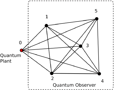
Figure 3: The plant observer network considered in the example.

For this example, the augmented plant-observer system can be described by the equations

$$\dot{x}_{a}(t)=A_{a}x_{a}(t),\mbox{ where }x_{a}(t)=\left[\begin{array}[]{l}z_{p}(t)\\ x_{o1}(t)\\ x_{o2}(t)\\ \vdots\\ x_{o5}(t)\end{array}\right]$$

and

$$A_{a}=\left[\begin{array}[]{lllllllllll}0&0&0&0&0&0&0&0&0&0&0\\ 0&0&10&0&0&0&0&0&0&0&0\\ 2&-10&0&2&0&2&0&2&0&2&0\\ 0&0&0&0&10&0&0&0&0&0&0\\ 2&2&0&-10&0&2&0&2&0&2&0\\ 0&0&0&0&0&0&10&0&0&0&0\\ 2&2&0&2&0&-10&0&2&0&2&0\\ 0&0&0&0&0&0&0&0&10&0&0\\ 2&2&0&2&0&2&0&-10&0&2&0\\ 0&0&0&0&0&0&0&0&0&0&10\\ 2&2&0&2&0&2&0&2&0&-10&0\end{array}\right].$$

Then, we can write

$$x_{a}(t)=\Phi(t)x_{a}(0)$$

where

$$\Phi(t)=e^{A_{a}t}.$$

Thus, the plant variable to be estimated $z_{p}(t)$ is given by

$$z_{p}(t) = e_{1}C_{a}\Phi(t)x_{a}(0)$$

$$= \sum_{i=1}^{2N+2}e_{1}C_{a}\Phi_{i}(t)x_{ai}(0)$$

where

$$C_{a}=\left[\begin{array}[]{ll}C_{p}&0\\ 0&C_{o}\end{array}\right],$$

$e_{1}$ is the first unit vector in the standard basis for $\mathbb{R}^{N+1}$, $\Phi_{i}(t)$ is the $i$th column of the matrix $\Phi(t)$ and $x_{ai}(0)$ is the $i$th component of the vector $x_{a}(0)$. We plot each of the quantities $e_{1}C_{a}\Phi_{1}(t),e_{1}C_{a}\Phi_{2}(t),\ldots,e_{1}C_{a}\Phi_{2N+1}(t)$ in Figure 4(a).

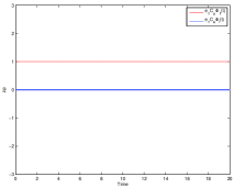
(a)

(b)

(c)

(d)

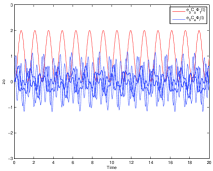
(e)

(f)

Figure 4: Coefficients defining (a) $z_{p}(t)$, (b) $z_{o1}(t)$, (c) $z_{o2}(t)$, (d) $z_{o3}(t)$, (e) $z_{o4}(t)$, and (f) $z_{o5}(t)$.

From this figure, we can see that $e_{1}C_{a}\Phi_{1}(t)\equiv 1$ and $e_{1}C_{a}\Phi_{2}(t)\equiv 0$, $e_{1}C_{a}\Phi_{2}(t)\equiv 0$, $\ldots$, $e_{1}C_{a}\Phi_{2N+2}(t)\equiv 0$, and $z_{p}(t)$ will remain constant at $z_{p}(0)$ for all $t\geq 0$.

We now consider the output variables of the quantum observer network $z_{oi}(t)$ for $i=1,2,\ldots,N$ which are given by

$$z_{oi}(t)=\sum_{j=1}^{2N+1}e_{i+1}C_{a}\Phi_{j}(t)x_{aj}(0)$$

where $e_{i+1}$ is the $(i+1)$th unit vector in the standard basis for $\mathbb{R}^{N+1}$. We plot each of the quantities $e_{i+1}C_{a}\Phi_{1}(t),e_{i+1}C_{a}\Phi_{2}(t),\ldots,e_{i+1}C_{a}\Phi_{2N+2}(t)$ in Figures 4(b) - 4(f).

To illustrate the time average convergence property of the quantum observer (20), we now plot the quantities $\frac{1}{T}\int_{0}^{T}e_{i+1}C_{a}\Phi_{1}(t)dt$, $\frac{1}{T}\int_{0}^{T}e_{i+1}C_{a}\Phi_{2}(t)dt$, $\ldots$, $\frac{1}{T}\int_{0}^{T}e_{i+1}C_{a}\Phi_{2N+2}(t)dt$ for $i=1,2,\ldots,N$ in Figures 5(a)-5(e). These quantities determine the averaged value of the $i$th observer output

$$z_{oi}^{ave}(T)=\frac{1}{T}\int_{0}^{T}\sum_{j=1}^{2N+1}e_{i+1}C_{a}\Phi_{j}(t)x_{aj}(0)dt$$

for $i=1,2,\ldots,N$.

(a)

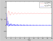
(b)

(c)

(d)

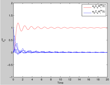
(e)

Figure 5: Coefficients defining the time average of (a) $z_{o1}(t)$, (b) $z_{o2}(t)$, (c) $z_{o3}(t)$, (d) $z_{o4}(t)$, and (e) $z_{o5}(t)$.

From these figures, we can see that for each $i=1,2,\ldots,N$, the time average of $z_{oi}(t)$ converges to $z_{p}(0)$ as $t\rightarrow\infty$. That is, the quantum observer network reaches a time averaged consensus corresponding to the output of the quantum plant which is to be estimated.

References

[1]
F. L. Lewis, H. Zhang, K. Hengser-Movric, and A. Das, Cooperative Control
of Multi-Agent Systems. London:
Springer, 2014.
[2]
G. Shi and K. H. Johansson, “Robust consusus for continuous-time multi-agent
dynamics,” SIAM Journal on Control and Optimization, vol. 51, no. 5,
pp. 3673–3691, 2013.
[3]
R. Olfati-Saber, “Kalman-consensus filter: optimality, stability, and
performance,” in Proceedings of the 48th IEEE Conference on Decision
and Control and 28th Chinese Control Conference, Shanghai, China, December
2009, pp. 7036–7042.
[4]
F. Ticozzi, L. Mazzarella, and A. Sarlette, “Symmetrization for quantum
networks: a continuous-time approach,” in Proceedings of the 21st
International Symposium on Mathematical Theory of Networks and Systems
(MTNS), Groningen, The Netherlands, July 2014, avaiable quant-ph, arXiv
1403.3582.
[5]
G. Shi, D. Dong, I. R. Petersen, and K. H. Johansson, “Consensus of quantum
networks with continuous-time markovian dynamics,” in Proceedings of
the 11th World Congress on Intelligent Control and Automation, 2014.
[6]
I. R. Petersen, “A direct coupling coherent quantum observer,” in
Proceedings of the 2014 IEEE Multi-conference on Systems and Control,
Antibes, France, October 2014, to appear, accepted 15 July 2014, also
available arXiv 1408.0399.
[7]
——, “A direct coupling coherent quantum observer for a single qubit finite
level quantum system,” in Proceedings of 2014 Australian Control
Conference, Canberra, Australia, November 2014, to appear, accepted 14 Aug
2014. Also arXiv 1409.2594.
[8]
Z. Miao and M. R. James, “Quantum observer for linear quantum stochastic
systems,” in Proceedings of the 51st IEEE Conference on Decision and
Control, Maui, December 2012.
[9]
M. R. James, H. I. Nurdin, and I. R. Petersen, “ control of linear
quantum stochastic systems,” IEEE Transactions on Automatic Control,
vol. 53, no. 8, pp. 1787–1803, 2008, arXiv:quant-ph/0703150.
[10]
A. J. Shaiju and I. R. Petersen, “A frequency domain condition for the
physical realizability of linear quantum systems,” IEEE Transactions
on Automatic Control, vol. 57, no. 8, pp. 2033 – 2044, 2012.
[11]
R. Hamerly and H. Mabuchi, “Advantages of coherent feedback for cooling
quantum oscillators,” Physical Review Letters, vol. 109, p. 173602,
2012.
[12]
L. A. D. Espinosa, Z. B. Miao, I. R. Petersen, V. Ugrinovskii, and M. R. James,
“Physical realizability of an open spin system,” in Proceedings of
the 20th International Symposium on Mathematical Theory of Networks and
Systems, Melbourne, July 2012.
[13]
J. Gough and M. R. James, “The series product and its application to quantum
feedforward and feedback networks,” IEEE Transactions on Automatic
Control, vol. 54, no. 11, pp. 2530–2544, 2009.
[14]
G. Zhang and M. James, “Direct and indirect couplings in coherent feedback
control of linear quantum systems,” IEEE Transactions on Automatic
Control, vol. 56, no. 7, pp. 1535–1550, 2011.