Abstract

Here, we propose a clustering technique for general clustering problems including those that have non-convex clusters. For a given desired number of clusters $K$, we use three stages to find a clustering. The first stage uses a hybrid clustering technique to produce a series of clusterings of various sizes (randomly selected). They key steps are to find a $K$-means clustering using $K_{\ell}$ clusters where $K_{\ell}\gg K$ and then joins these small clusters by using single linkage clustering. The second stage stabilizes the result of stage one by reclustering via the ‘membership matrix’ under Hamming distance to generate a dendrogram. The third stage is to cut the dendrogram to get $K^{*}$ clusters where $K^{*}\geq K$ and then prune back to $K$ to give a final clustering. A variant on our technique also gives a reasonable estimate for $K_{T}$, the true number of clusters.

We provide a series of arguments to justify the steps in the stages of our methods and we provide numerous examples involving real and simulated data to compare our technique with other related techniques.

Keywords: hybrid clustering, $K$-means, single linkage, non-convex clusters, stability

1 Introduction

Clustering is an unsupervised technique used to find underlying structure in a dataset by grouping data points into subsets that are as homogeneous as possible. Clustering has many applications in a wide range of fields. No list of references can be complete, however, three important recent references are [1], [2] and [3].

Arguably, there are three main classes of clustering algorithm: Centroid-based, Hierarchical, and Partitional. Centroid-based refers to $K$-means and its variants. Hierarchical comes in two main forms, divisive and agglomerative. Partitional comes in three main forms graph-theoretic, spectral, and model-based. Because the scope of clustering problems is so big, all of these procedures have limitations. So, each major class of clustering procedures has its strengths and weakness even if, in some cases, these are not mapped out very precisely.

The justification for the new method presented here is that it combines two classes of methods (centroid-based and agglomerative hierarchical) with a careful treatment of influential data points and (i) is not limited by convexity or (ii) as dependent on subjective choices of quantities such as dissimilarities. That is, we combine several clustering techniques and principles in sequence so that one part of the technique may correct weaknesses in other parts giving a uniform improvement – not necesarily decisively better than other methods in particular cases, but rarely meaningfully outperformed. In particular, we have not found any examples in which our clustering method is outperformed to any meaningful extent. The examples presented here dramatize this since most of them are very diffucult for any clustering method. One consequence of this is that our procedure is well designed for non-convex clusterings as well convex ones.

A further benefit of our clustering method is that we can give formal conditions ensuring that the clustering will be correct for special cases. That is, we prove a theorem ensuring that the basal sets cover the regions in a clustering problem, in the limit of large sample size and use this to establish a corollary ensuring that the final clustering from our method, at least in simple cases, will be correct. We also give formal results ensuring that the conditions of our main theorem can be satisfied in some simple but general cases. To the best of our knowledge, there are no techniques, except for $K$-means, for which theoretical results such as ours can be established.

To fix notation, we assume $n$ independent and identical (IID) outcomes $x_{i},~{}i=1,\ldots,n$ of a random variable $X$. The $x_{i}$’s are assumed $m$-dimensional and written as $(x_{i1},\dots,x_{im})$ when needed. We denote a clustering of size $K$ by ${\cal{C}}_{K}=(C_{K1},\ldots,C_{KK})$; effectively we assume that for each $K$ only one clustering will be generated.

For a given $K$, we start by drawing a random $K_{b}$, $b=1,\ldots,B$ from a distribution that ensures a variety of reasonable clustering sizes will be searched. Then, the generic steps are as follows.

1. Hybrid clustering: Create $K_{\ell}$ clusters by $K$-means. Then use single linkage (SL) clustering to take unions of the $K_{\ell}$ cluster to get clusterings of size $K_{b}$.

2. Stabilization: Repeat stage one $B$ times; the result is $B$ clusterings with sizes $K_{1},\ldots,K_{B}$. From these clusterings, form a pooled $n\times\sum_{b}K_{b}$ membership matrix $M$. Since each row of $M$ corresponds to an $x_{i}$ and is a vector of zeros and ones of length $\sum_{b}K_{b}$, the Hamming distance $H(x_{i},x_{j})$ between any two rows can be found and is between one and $B\sum_{b}K_{b}$. These Hamming distances give a dissimilarity so that SL clustering can again be applied.

3. Choosing a clustering: Use a ‘grow-and-prune’ approach on the dendrogram from Stage 2. Cut the dendrogram at some dis-similarity value smaller than $H_{K}$, the value of the dis-similarity that gives $K$ clusters. The $K^{*}$ clusters are then merged to form $K$ clusters after ignoring any clusters that are too small.

The last stage involves possibly two reclusterings: One to merge the larger clusters down to $K$ clusters and a second to merge the small clusters into these $K$ clusters. The definition of small clusters requires the use of a cutoff value $\alpha$, here taken to be 0.05; details are in Sec. 2.

In Step 1), there is a range of choices for dis-similarity to be used in the SL clustering. The usual dis-similarity, namely, defining the minimum distance between two sets the be the shortest path length connecting them, is one valid choice. As seen below, however, it is most effective when the data are generated from a probability measure $P$ that has disjoint closed components each the closure of an open set. When the components of $P$ are not disjoint, we have found it advantageous to use a robustified form of the minimum distance between two sets, namely the 20th percentile of the distances between the points in the two sets. This is discussed further in Subsec. 3.2

There are precedents for the kind of hybrid clustering described in stages 1) and 2) that combines two or more distinct clustering techniques. Perhaps the closest is [4] Their central idea is to create many clusterings of different sizes (by $K$-means) that can be pooled via a ‘co-association matrix’ that weights points in each clustering according their membership. This matrix can then be modified (take one minus each entry) to give a dis-similarity so that single-linkage clustering can be used to give a final clustering. [4] refer to this as evidence accumulation clustering (EAC) because they are pooling information over a range of clusterings. EAC differs meaningfully from our technique in three ways. First, in our technique we choose a single $K_{\ell}$ while EAC uses a range of cluster sizes. Second, we ensemble (and hence stabilize) directly by membership in terms of Hamming distance whereas EAC ensembles by a co-association. Third, our procdure uses an extra step of growing and pruning a dendrogram (see Step 5 in Algoirthm #1) that is akin to an optimization over ‘main’ clusters. Our ‘fine-tuning’ of their technique seems to give better results.

Another technique that is conceptually similar to ours is due to Chipman and Tibshirani [5], hereafter CT. First, in a ‘bottom-up stage’, small sets of points that are not to be separated are replaced by their centroids. Then, in a ‘top-down stage’ the remaining points are clustered divisively to give big clusters. Then, the bottom up and top-down stages are reconciled to give a final clustering. Our proposed technique differs from CT in four key ways. First, we use $K$-means in place of CT’s ‘mutual clusters’. Second, we use single linkage where CT uses average linkage. Third, our technique has a stabilization stage. Fourth, our technique uses a ‘grow and prune’ strategy, unlike CT. So,it is unclear how well CT performs when the true clusters are non-convex.

A third technique, conceptually related to ours but nevertheless very different, is due to Karypis et al. ([6]). This technique, often called CHAMELEON, rests on a graph theoretic analysis of the clustering problem and uses two passes over the data. The first is a graph partitioning based algorithm to divide the data set into a collection of small clusters. The second pass is an agglomerative hierarchical clustering based on connectivity (a graph-theoretic concept) to combine these clusters. Our method differs from [6] in four key ways. First, we use $K$-means instead of graph partitioning. Second, we simply use single linkage whereas [6] combines small clusters based on both closeness and relative interconnectivity. Third, our technique has a stabilization stage to manage cluster boundary uncertainty. Fourth, our technique explicitly uses a ‘grow and prune’ strategy permitting a ‘look ahead’ to more clusters than necessary. By contrast, CHAMELEON has an elaborate optimization. On the other hand, both can find non-convex clusters.

To the best of our knowledge, the earliest explicit proposal for hybrid methods is in [7] who observed that using $K$-means with $K$ too large and single linkage may enable a technique to find nonconvex clusters.

In addition to proposing a new hybrid clustering technique (Algorithm #1) we present a way to estimate the correct value $K_{T}$ of $K$ in Algorithm #2. Essentially, we combine the first three steps of algorithm #1 with a modification of [4].

The rest of this paper is organized as follow. In Sec. 2 we present our two algorithms for clustering and estimating $K_{T}$. In Sec. 3 we provide justifications for some of the steps in our algorithms. For the steps where we are unable to provide theory, we provide methodological interpretations as a motivation for their use. In Sec. 4 we present our numerical comparisons. Our concluding remarks are in Sec. 5.

2 Presentation of techniques

We begin with Algorithm #1 that formalizes our generation of clusterings. It has five steps and five inputs: the number $K$ of clusters to be in the final clustering, a number $K_{max}$ to be the largest number of clusters that we would consider reasonable, a number $B$ of iterations of our initial hybrid clustering technique, a number $K_{\ell}\gg K$ of smaller clusters that will be concatenated to larger clusters, and a value $\alpha$ to serve as a cutoff for the size of a cluster as measured by the proportion of how many of the $K_{\ell}$ clusters had to be combined to create it. In practice, setting $K_{\ell}=\lfloor n/5\rfloor$ worked reasonably well; however, $\lfloor n/5\rfloor$ is an arbitrary choice and we found that adding a layer of variability by choosing $K_{\ell}$ according to a $DUnif[\lfloor n/4\rfloor,\lfloor n/6\rfloor]$ gave improved results. Separately, we also found that larger values of $K_{max}$ seemed to require larger values of $B$ to get good results. We address the choice of $B$ and $K_{max}$ later in Sec. 4. In our work here, we merely set $\alpha=.05$. This ensured that we got at least $K$ clusters in our examples. Loosely, the more outliers or clusters there are, the smaller one should choose $\alpha$. So, effectively, given Algorithm #1, only $K$ must be specified. The specification of $K$ is done separately in Algorithm #2.

We begin with our clustering algorithm given in the column to the right.

Algorithm 1 Stablized Hybrid Clustering (SHC)

1. Given $K$, start by drawing a value of $K_{\ell}$ and then drawing a value of $K_{b}\sim DUnif(2,K_{max})$ where $K_{max}<K_{\ell}$, for $b=1,\ldots,B$. For each $K_{b}$, do the following with randomly generated initial conditions to obtain ${\cal{C}}(K_{b})=\{C_{b1},\ldots,C_{bK_{b}}\}$:

   • Use standard $K$-means clustering (or any partitional technique) to generate a clustering of size $K_{\ell}$ ‘basal’ clusters.

   • Next, use single linkage clustering (or any agglomerative technique) to merge the $K_{\ell}$ basal clusters to get a clustering ${\cal{C}}_{K_{b}}$.

2. For ${\cal{C}}(K_{1})$, let $M_{1}=(\chi(s,t))_{s=1,\ldots,n;t=1,\ldots,K_{1}}$ be the $n\times K_{1}$ membership matrix with entries $\chi(s,t)=\begin{cases}1&x_{s}\in C_{K_{1},t}\\ 0&x_{s}\notin C_{K_{1},t}.\end{cases}$ Doing the same for the rest of the ${\cal{C}}(K_{b})$’s generates membership matrices $M_{1},\ldots,M_{B}$ for clusterings ${\cal{C}}(K_{2}),\ldots,{\cal{C}}(K_{B})$, respectively. Concatenating $M_{b}$’s gives the overall membership matrix $M(B)=[M_{1},\ldots,M_{B}]$.

3. From the $n\times\sum_{b}K_{b}$ overall membership matrix $M(B)$ we construct a dissimilarity matrix using Hamming distance. Let $S=\sum_{b}K_{b}$. That is, the $i$-th and $j$-th rows in $M(B)$ are of the form $x_{i}=(x_{i,1},\ldots,x_{i,S})$ and $x_{j}=(x_{j,1},\ldots,x_{j,S})$ and so give dis-similarities $d_{ij}=d(x_{i},x_{j})=\sum_{m=1}^{S}{\sf I}(x_{im},x_{jm})$ where ${\sf I}(x_{im},x_{jm})=1$ if $x_{im}\neq x_{jm}$ and zero otherwise. So, $d_{ij}$ is the number of entries in $x_{i}$ and $x_{j}$ that are different and $0\leq d_{ij}\leq S$. Let $D=(d_{ij})$ be the resulting matrix.

4. Given $D$, use SL clustering to generate a vertical dendrogram with leaves at the bottom and dis-similarity values on the $y$-axis. Since $K$ is given, it corresponds to a dis-similarity value $H_{K}$ on the vertical axis, namely, $H_{K}$ is the maximum dis-similarity associated with $K$ clusters. Now, there will be $K$ lines or branches on the dendrogram that cross $H_{K}$. Let the lengths of these lines from $H_{K}$ down to the next split be denoted $h_{1},\ldots,h_{K}$. Cut the dendrogram at $H_{K}+\bar{h}$ and let $K^{*}$ be the number of clusters at that value.

5. Write $K^{*}=K+v$ with $v\geq 0$. If $v=0$, the clustering from Step 4 of size $K$ is the final clustering. If $v\geq 1$, write $v=v_{1}+v_{2}$ where $v_{2}$ is the number of clusters in the clustering ${\cal{C}}_{K^{*}}$ for which $\#(C_{K^{*}j})/n\leq\alpha$. In the case that $K$ clusters of size at least $\alpha$ do not exist, $\alpha$ is adjusted downward until $K$ such clusters exist. Ignore these $v_{2}$ clusters and using SL (under the corresponding submatrix of $D$) recluster the points in the remaining $(K+v_{1})$ clusters to reduce them to $K$ ‘main’ clusters. Then, use SL clustering again to assign the points in the $v_{2}$ clusters to the $K$ ‘main’ clusters to give the final clustering of size $K$.

For brevity, we refer to Algorithm #1 as SHC.

In SHC, we have specified the use $K$-means in the first part of Step 1 but left open which dissimilarity to use in Step 2. This is intentional because we can establish theory for our method that suggests the usual minimum distance dissimilarity is best when the components of $P$ are separated (convex or not); however, a dissimilarity between sets based on 20th percentile of the distance between their points works better when the separation is not clear or entirely absent. In our examples below we denote these dissimilarities by writing SHCm (minimal) and SHC20 (20th percentile).

Note that the number of clusters $K^{*}$ is defined internally to the algorithm in Step 4. The idea is to get a tree that is slightly larger than cutting at $H_{K}$, i.e., to let the algorithm search an extra few steps ahead for good clusters. In Step 5, any extra clusters that are found but not helpful are pruned away. The intuition behind the choice of $K^{*}$ is that the level of the dissimilarity it represents identifies the point at which chaining begins to affect the clustering procedure negatively.

Algorithm #1 can serve as the basis for another algorithm to estimate $K_{T}$. We add an extra step derived from the method for choosing $K$ in [4]. Recall that [4] considered a set of ‘lifetimes’ that were lengths in terms of the dissimilarity. These were the distances between the values on the vertical axis at which one could cut a dendrogram so as to get a collection of clusters with the property that at least one of the clusters emerges precisely at the value on the vertical axis at which the horizontal line was drawn. [4] then cut the dendrogram at the dis-similarity that corresponds to the maximum of these vertical distances to choose the number of clusters. Algorithm #2 extends this method by using it once, removing some clusters, and then using it again.

Our general procedure is given in Algorithm #2, next page.

Algorithm 2 Estimate of $K_{T}$ (EK)

1. Use Steps 1-3 from Algorithm #1 to obtain $D$.

2. Form the dendrogram for the data under $D$ using SL.

3. Use the [4] technique to find the two largest lifetimes.

4. For each of the two largest lifetimes, cut the dendrogram at that lifetime and examine the size of the clusters. Remove clusters that are both small (containing less that $\alpha$100% of the data) and split off at or just below $H_{K}$. This gives two sub-dendrograms, one for each lifetime.

5. For each of the sub-dendrograms, cut at $H_{K}$. This gives two numbers of clusters. Take the mean of these two numbers of clusters as the estimate of the correct number of clusters.

For brevity, we refer to Algorithm #2 as EK.

3 Justification

In this section we provide motivation, interpretation, and properties of the steps in the two algorithms we have proposed.

3.1 $K$-means with large $K_{\ell}$

Let the probability measure $P$ have density $p$ and assume that $p$ only takes values zero and a single, fixed constant. The places where $p$ assumes a nonzero value are the clusters of $P$. Our first result shows that the support of $p$ can be expressed as a disjoint union of small clusters in the limit of large $n$. Let $A\bigtriangleup B$ denote the symmetric difference between sets $A$ and $B$ and for any set $A$, let ${\sf diam}(A)=\sup_{x,y\in A}d(x,y)$ be the diameter of $A$. Now, given data $x^{n}=\{x_{1},\ldots,x_{n}\}$ write $\hat{\cal{C}}_{K}=(\hat{C}_{K1},\ldots\hat{C}_{KK})$ to be a clustering of $x^{n}$ into $K$ clusters. Our result is the following.

Theorem 1.

Suppose the following assumptions are satisfied:

1. $\forall K,m~{}\exists~{}C_{Km}$ so that

   $$P(\hat{C}_{Km}\bigtriangleup C_{Km})\rightarrow 0$$

   in $P$-probability as $n\rightarrow\infty$.

2. For any $m$,

   $$\sup_{m=1,\dots,K}{\sf diam}(C_{Km})\rightarrow 0$$

   as $K\rightarrow\infty$.

3. For each $m$ and $K$, $P(C_{Km})>0$.

4. The support of $p$, ${\sf supp}(P)$, consists of finitely many disjoint open sets with disjoint closures having smooth boundaries.

5. The random variable $X$ generating $x^{n}$ is bounded.

Then for any fixed $m$, along any sequence of sets $C_{Km}$ with $P(diam(C_{Km}))>0$, there is a $z\in\overline{\sf Supp}(P)$, the support of $P$, so that

$$E(X|\widehat{C}_{Km})\longrightarrow z,$$ (1)

as $n$ increases first and $K$ increases second, at suitable rates.

Proof.

Consider a sequence $\langle\hat{C}_{Km}\rangle\mid_{K=1}^{\infty}$ for which $P(C_{Km})>0$; this is possible by items 1) and 3). By item 2), $P(C_{Km})\rightarrow 0^{+}$.

Step 1: For such a sequence,

$$E(X|\widehat{C}_{Km})-E(X|C_{Km})\overset{P}{\longrightarrow}0:$$

Begin by writing

$$E(X|\widehat{C}_{Km})-E(X|C_{Km})$$ (3)

$$= \int_{\widehat{C}_{Km}}\frac{XdP}{P(\widehat{C}_{Km})}-\int_{C_{Km}}\frac{XdP}{P(C_{Km})}$$

$$= \int_{\widehat{C}_{Km}}\frac{XdP}{P(\widehat{C}_{Km})}-\int_{\widehat{C}_{Km}}\frac{XdP}{P(C_{Km})}$$

$$+\int_{\widehat{C}_{Km}}\frac{XdP}{P(C_{Km})}-\int_{C_{Km}}\frac{XdP}{P(C_{Km})}.$$

Since $X$ is bounded, term (3) goes to zero as $n\rightarrow\infty$ by the Dominated Convergence Theorem since $I_{C_{Km}}-I_{\widehat{C}_{Km}}\rightarrow 0$ in $P$-probability under item 1).

To deal with term (3), write it as

$$\int_{I_{\widehat{C}_{Km}}}\left(\frac{1}{P(\widehat{C}_{Km})}-\frac{1}{P(C_{Km})}\right)XdP.$$ (4)

Since $X$ is bounded by $M$, say, the absolute value of term (4) is bounded by

$$MP(\widehat{C}_{Km})\left|\frac{1}{P(\widehat{C}_{Km})}-\frac{1}{P(C_{Km})}\right|$$

$$=M\left|1-\frac{P(\widehat{C}_{Km})}{P(C_{Km})}\right|.$$ (5)

Now, by assumption 1, with probability at least $1-\eta$, for any $\eta>0$, as $n\rightarrow\infty$ we have

$$\frac{P(\widehat{C}_{Km})}{P(C_{Km})}\longrightarrow 1.$$

So, the factor in absolute value bars in (5) can be made less than any pre-assigned positive number, for instance, $\eta/M$, giving that (4) can be made arbitrarily small as $n\rightarrow\infty$. Consequently,

$$E(X|\widehat{C}_{Km}) = E(X|\widehat{C}_{Km})\pm E(X|C_{Km})$$

$$= o_{P}(1)+E(X|C_{Km})$$

and Step 1 is complete.

Step 2: By item 2), $\exists z$ such that $C_{Km}\rightarrow\{z\}$. So, by Step 1, as $n\rightarrow\infty$

$$E(X\mid\hat{C}_{Km})\rightarrow z$$

in $P$-probability. Now, to prove the theorem, it remains to show $z\in\overline{{\sf supp}(P)}$.

By way of contradiction, suppose $z\notin\overline{{\sf Supp}(P)}$. Then, since $\overline{{\sf Supp}(P)}$ is a closed set by item 4), its complement is open and hence $\exists\epsilon>0$ so that $B(z,\epsilon)\subset\overline{{\sf Supp}(P)}^{c}$, where $B(z,\epsilon)$ indicates a ball centered at $z$ of radius $\epsilon$. However, consider a sequence of sets $C_{Km}$ for some fixed $m$ with

$$\forall K:P(C_{Km})>0;$$

such a sequence must exist for some $m$ by Item 3). By Item 2), we have that

$${\sf diam}(C_{Km})\rightarrow 0~{}\hbox{as}~{}K\rightarrow\infty.$$ (6)

So, $\exists K_{0}$ such that $\forall K\geq K_{0}$,

$$C_{Km}\subset B(z,\epsilon),$$

and therefore $P(C_{Km})=0$ by letting $n$ and $K$ increase at appropriate rates, a contradiction. Hence, $z\in\overline{{\sf Supp}(P)}$, establishing the theorem. ∎

The utility of the theorem stems mostly from the following corollary.

Corollary 1.

There exists a $K_{0}$ so that for $K\geq K_{0}$, there are $m_{1},\ldots,m_{\ell}\leq K$ for sole $\ell$ with

$$P\left({\sf Supp}(P)\bigtriangleup\left(\cup_{j=1}^{l}\widehat{C}_{Km_{j}}\right)^{c}\right)<\epsilon.$$ (7)

That is, there are rates at which $n\rightarrow\infty$, $K\rightarrow\infty$ and $\epsilon\rightarrow 0^{+}$, so that in a limiting sense

$${\sf Supp}(P)\approx\cup_{j=1}^{l}\widehat{C}_{Km_{j}}.$$ (8)

This corollary gives conditions under which the procedure of choosing $K$ too large, in $K$-means for instance, ensures that the union of the clusters for that $K$ very closely approximates the support of $X$, regardless of whether the support is convex or not. 5disjoint open sets.

Since assumptions 3), 4) and 5) are straightforward to assess, we provide sufficient conditions for assumptions 1) and 2) for the special case of $K$-means clustering.

To do this for assumption 1), recall that $K$-means uses the Euclidean distance to define the dis-similarity $d(x,x^{\prime})$ for points $x$ and $x^{\prime}$. Formally, in the limit of large sample sizes, let $\mu_{k},~{}k=1,\ldots,K$ be the means of unknown classes $C_{Km}$ under clustering ${\cal{C}}_{K}=\{C_{K1},\ldots,C_{KK}\}$ and let $C$ be the membership function that assigns data points $x_{i}$ to clusters i.e., $C(i)=m\Leftrightarrow x_{i}\in C_{Km}$ under the clustering ${\cal{C}}_{K}$. Then the $K$-means clustering is the ${\cal{C}}_{K}$ that achieves

$$\text{min}_{K}~{}\text{min}_{\mu_{1},\ldots,\mu_{K}}~{}\sum_{k=1}^{K}\sum_{i:C(i)=k}\|x_{i}-\mu_{k}\|^{2}.$$ (9)

(Strictly speaking, the objective function in (9) should be written in its limiting form

$$\sum_{k=1}^{K}~{}\int_{C_{Km}}\|x-\mu_{Km}\|^{2}~{}dP(x)$$ (10)

with the constraints $\mu_{Km}=\int_{C_{Km}}X~{}dP$.)

Under the $K$-means optimality criterion, given $K$ there are $\mu_{1},\ldots,\mu_{K}\in{\sf Supp}(P)$ such that the minimum in (9) (or (10)) can be written as

$$\sum_{k=1}^{K}\int_{C_{Km}}(x-\mu_{Km})^{2}~{}P(dx),$$

with the property that

$$x\in C_{Km}\Longleftrightarrow d(x,\mu_{Km})\leq d(x,\mu_{K\ell}),\ell\neq k.$$ (11)

Defining the centroid of $C_{Km}$ as

$$\mu_{Km}=E\left({x}\mid{x}\in C_{Km}\right)=\int_{C_{Km}}{x}~{}P(dx),$$

with corresponding estimate defined as

$$\widehat{\mu}_{Km}=E\left({x}\mid{x}\in\widehat{C}_{Km}\right)=\int_{{\widehat{C}_{Km}}}{x}~{}P(dx),$$

we can quote the following result.

Theorem 2.

Under various regularity conditions, as $n\rightarrow\infty$, the $K$-means clustering $\widehat{\cal{C}}_{K}$ is consistent for ${\cal{C}}_{K}$. In particular,

$$\widehat{\mu}_{Km}\longrightarrow\mu_{Km},~{}a.s.$$ (12)

Proof.

See Pollard (1981). ∎

Since $K$-means is a centroid-based clustering, we have that

$$x\in\widehat{C}_{Km}\Longrightarrow\forall\ell\neq m~{}d(x,\widehat{\mu}_{Km})\leq d(x,\widehat{\mu}_{K\ell}),$$

so combining this with (11) we get that

$$\widehat{\mu}_{Km}\longrightarrow\mu_{Km}\Longleftrightarrow P(\widehat{\cal{C}}_{K}\bigtriangleup{\cal{C}}_{K})\longrightarrow 0,$$ (13)

i.e., assumption 1) is satisfied.

Turning to assumption 2), consider the following example with $K$-means to understand the intuition behind it. Suppose a data set is generated as two clusters of the same number of outcomes, one with high variance and one with low variance, see the upper left panel in Fig. 1. Then, applying $K$-means with increasing $K$, e.g., $K=2,4,10,14,18,20,24,30$ in Fig. 1 shows that $K$-means partitions the two clusters more and more finely but continually assigns more clusters to the high variance data. In this context, assumption 2) means that as $n$ increases, the clusters will appear to ‘fill in’ yielding $K$ regions with non-void interior for each $K\geq 2$ even if the $n$ required for a given $K$ increases with $K$.

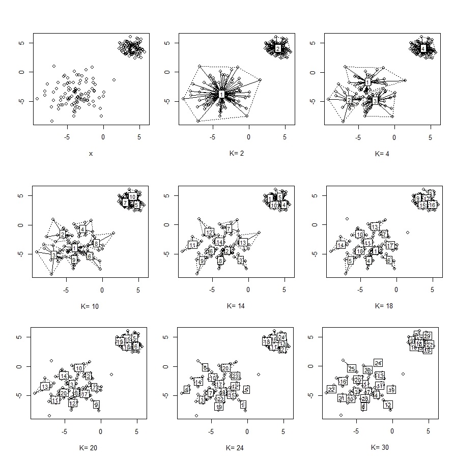
Figure 1: Plots of two clusters using different choices of $K$ to see how clustering divides the true clusters.

To begin formalizing this intuition, write

$$WSS=\sum_{k=1}^{K}\sum_{i:C(i)=k}\|x_{i}-\mu_{k}\|^{2},$$ (14)

recognizable as the ‘within clusters’ sum of squares. In the one-dimensional case, suppose $2n$ data points are drawn, $X^{*}_{1}=(X_{1},\ldots,X_{n})\sim Unif[0,a]$ and $X^{*}_{2}=(X_{n+1},\ldots,X_{2n}\sim Unif[2a,4a]$. Clearly, $X_{1}$ represents a low diameter component and $X_{2}$ represents a high diameter component. If we seek a $K$-means clustering for $K=2$, it is clear that $X^{*}_{1}$ and $X^{*}_{2}$ should be found. However, consider $K=3$. There are two natural clusterings. The first is to split $X^{*}_{1}$ into two clusters of equal size, say $C_{1}$ and $C_{2}$ letting $C_{3}=\{X^{*}_{2}\}$. The other is the reverse: Let $C_{1}=\{X^{*}_{1}\}$ and split $X^{*}_{2}$ into two clusters of equal size, say $C_{2}$ and $C_{3}$. It is easy to verify that the population value of WSS for the first clustering is $(9/24)a^{2}$ while for the second clustering it is $(3/24)a^{2}$. This means the second clustering, splitting the high diameter component, gives a smaller WSS. Since $K$-means chooses the mean of WSS over the number of clusters, in this case, $K$-means would choose the second clustering.

The example can be continued for higher $K$, higher $K_{T}$, and other distributions continuing to show that $K$-means tends to split the largest cluster until it is worthwhile to split the smaller cluster and then resumes splitting the larger cluster, and so on. A consequence of this is that $\hat{C}_{Km}$ tends to decrease in size as $K$ increases and this suggests that $C_{Km}$ will similarly decrease as assumed in Item 2) as $n\rightarrow\infty$. We state a version of this in the following.

Proposition 1.

Suppose a clustering method continually splits the largest cluster on the population level as $K$ increases. Then, given $\delta>0$, there is a $K_{0}$ so that

$$k>K_{0}\Longrightarrow{\sf diam}(C_{k})<\delta.$$ (15)

Proof.

Let $\{\mu_{K1},\ldots,\mu_{KK}\}$ be the centers of the optimal clusters and write

$$C_{Km}=\{x:|x-\mu_{Km}|<|x-\mu_{K\ell}|\}$$

for $\ell\neq m$. Let

$$\delta_{0}=\max\{{\sf diam}(C_{Km}):m=1,\ldots,K\}.$$

Then, for $K^{\prime}$ large enough,

$$\max\{{\sf diam}(\widehat{C}_{K^{\prime}m}):m=1,\ldots,K^{\prime}\}\leq\frac{\delta_{0}}{2}.$$

Since this process can be repeated the proposition is established. ∎

Taken together, the results of this subsection justify the $K$-means part of Step 1) of Algorithm #1.

3.2 Merging the ’basal’ clusters

Next we turn to justifying the use of single linkage (SL) in the second part of Step 1 in Algorithm # 1. Recall, SL means that we merge sets that are closest i.e., given a distance $d$ on, say, $C_{K1},\dots,C_{KK}$, SL clustering merges the two sets that achieve

$$\min_{m,m^{\prime}=1,\dots,K;m\neq m^{\prime}}d(C_{Km},C_{Km^{\prime}}).$$

The question that remains is how to choose $d$. Here we use two choices. The first is to write $d$ as

$$d_{usual}(C_{Km},C_{Km^{\prime}})=\min_{x\in C_{Km},x^{\prime}\in C_{Km^{\prime}}}d(x,x^{\prime}),$$ (16)

where $d$ is a metric e.g., Euclidean, i.e., $d_{usual}$ gives the distance between two sets as the minimum over the distances between their points.

However, being an order statistic, (16) can be affected by extreme values in the data set. So, we stabilize $d_{usual}(C_{Km},C_{Km^{\prime}})$ by replacing it with the 20th percentile of the distances between points in $C_{Km}$ and $C_{Km^{\prime}}$. That is, for $m\neq m^{\prime}$, we find the distances

$$\{d(x,x^{\prime}):x\in C_{Km},x^{\prime}\in C_{Km^{\prime}}\},$$

take their order statistics, and find the approximately $\lfloor.2\#(C_{Km})\#(C_{Km^{\prime}})\rfloor$ order statistic. (Finding a non-integer order statistic is done internally to the R program using linear interpolation.) We call the resulting dissimilarity $d_{20}$, i.e.,

$$d_{20}(C_{Km},C_{Km^{\prime}})=20-\mbox{th percentile of}~{}$$

$$\{d(x,x^{\prime}):{x\in C_{Km},x^{\prime}\in C_{Km^{\prime}}}\}$$ (17)

to indicate it is based on the 20th percentile of the distances between points in the two sets. Thus, with $d_{20}$ we are using single linkage with respect to a dissimilarity that should be robust against extreme values. Other percentiles such as the fifth or tenth can also be used, but they gave values between $d_{usual}$ and $d_{20}$ in the examples we studied. It seemed from our work that $d_{20}$ gave the best resuts in cases where $d_{usual}$ did not.

For the sake of completeness we next give conditions under which $d_{usual}$ can be expected to perform well. We are unable to demonstrate this for $d_{20}$ but suggest there will be an analogous result since using $d_{20}$ gave results that were essentially never worse (and sometimes better) than $d_{usual}$.

Suppose $\overline{\sf Supp}(P)$ consists of $K_{T}$ disjoint regions each being the closure of an open set, assumed disjoint from the other open sets. Let $\delta$ be the minimum distance between points in disjoint components, i.e.,

$$\delta=\min_{m,m^{\prime}=1,\ldots,K_{T};m\neq m^{\prime}}\min_{x\in C_{m},x^{\prime}\in C_{m^{\prime}}}d(x,x^{\prime}).$$

If $n$ and $K$ are chosen so large that all the $\hat{C}_{Km}$’s for $m=1,\ldots,K$ have ${\sf diam}(\hat{C}_{Km})<\delta/3$ (any number strictly less than $\delta$ will suffice), choose a regular grid $G$ of points in $\overline{\sf Supp}(P)$ so that the distance between two adjacent points on the same axis is less than $(1/2)(\delta/3)$. This ensures that each $\hat{C}_{Km}$ has at least one grid point in it. The points in $G$ are essentially a perfectly representative set of $\overline{\sf Supp}(P)$ and hence of $P$. Now, if we apply SL with $d_{usual}$ to the points in $G$ we will always put points or subsets in the same component together before we merge points or subsets of any two distinct components. That is, the metric on $G$ ensures that the closest point to any other point will always be in the same component if possible. So, we have proved the following theorem.

Theorem 3.

If the components of $\overline{\sf Supp}(P)$ are disjoint there is a cut point in the dendrogram of the SL merging under $d_{usual}$ of the points in $G$ that separates the components perfectly.

Now, if $n$ is large enough, the data set can be taken as perfectly representative of $\overline{\sf Supp}(P)$ and hence of $P$, i.e., it is a good approximation to $G$ in the sense of filling out all the components of $P$. Hence, it follows that SL using $d_{usual}$ can perfectly separate the components of $\overline{\sf Supp}(P)$, and hence of $P$, in a limiting sense. This does not require convexity of the components of $P$, only that the data points can be regarded as essentially a perfect representation of $P$.

Note that one of the key hypotheses of this theorem forces the components of $P$ to be separated. In fact, this is often not the case – components may touch each other at individual points or may be linked by a very thin short line. In these cases, the components of ${\sf Supp}(P)$ may not have disjoint closures or the closure of the components may not give $\overline{\sf Supp}(P)$, respectively. When assumption 4 of Theorem 1 is satisfied, we have found that $d_{usual}$ works well: In a limiting sense, two basal sets from the same component will always be joined before either is joined to another component. However, when hypothesis 4 of Theorem 1 is not satisfied, $d_{usual}$ does not have this property. In these cases, we have found $d_{20}$ to work better; this is seen in Subsec. 4.2.1. It should be noted that the examples in Subsecs. 4.2.3 and 4.2.4 also do not seem to satisfy hypothesis 4 but for these cases $d_{usual}$ and $d_{20}$ give comparable results. We regard this as a reflection of the fact that hypothesis 4 is necessary but not sufficient for the conclusion of Theorem 1. Also, although not shown here, we examined our clustering technique using $d_{5}$ and $d_{20}$ in the sense of (17) but found they were outperformed by at least one of $d_{usual}$ or $d_{20}$. One point in favor of $d_{usual}$ is that it is interpretable in that two points are in the same cluster merely if they are close enough, unlike $d_{20}$.

Why does the 20-th percentile work well in cases where hypothesis 4 is not satisfied? While we do not have a formal argument, the intuition may be expressed as follows. If hypothesis 4 is not satisfied and the clusters are highly non-convex $d_{usual}$ will be much more sensitive to the boundary values of the clusters than $d_{20}$. Consequently, there may be overly influential data points – data points that are valid but far from other data points – that will affect the sequence of merges of the basal clusters in ways that are not representative of the support of $P$. Using $d_{20}$ in place of $d_{usual}$ reduces the influence of these data points eliminating distortions of the path by which basal clusters are merged. We do not have a rule for when to use $d_{usual}$ versus $d_{20}$, however, the presence of extreme points (as opposed to outliers) is a good indicator that $d_{20}$ should be preferred and this is consistent with all our examples. Indeed, the examples in Subsecs. 4.2.3 and 4.2.4, where $d_{usual}$ and $d_{20}$ give equivalent results, do not have clusters with extreme points.

3.3 Using the overall membership matrix

In Steps 2 and 3 of algorithm #1, a composite membership matrix $M(B)$ for $B$ clusterings is defined. Then, single linkage clustering is applied to the rows of $M(B)$ in Step 4. Because $D$ is absed on $M(B)$ our results should be robust results because by using several random starts for the clustering and looking only at which cluster a data point is in, we are ensuring that the final clustering is a sort of ‘consensus clustering’ representing what is invariant under two sorts of randomness – randomness of the clustering and random noise in the data points themselves.

Our use of the matrix $M(B)$ means our method may be regarded as an ensemble approach. Each set of columns in $M(B)$ represents a clustering and pooling over clusterings in step 4 effectively means that we are analyzing $B$ different clustering structures for the data. The analog of ensembling the matrices is played by single linkage which groups similar clusterings together. The result is that the final clustering is stabilized.

3.4 Growing and pruning

In Step 4, algorithm #1 grows a dendrogram of size $K^{*}$ by single linkage. In fact, $K^{*}$ may be bigger than the size $K$ of the desired clustering. In such cases, the dendrogram ‘grown’ is too large and must be pruned back. This is done in Step 5.

The benefit of this is that by growing a dendrogram a little larger than required, the method may look one or more splits further along so that outliers or other aberrant points may be removed. The outliers or other aberrant points are in the $v_{2}$ small clusters that are removed before the data are reclustered. Leaving out the $v_{2}$ small clusters means that the resulting clustering should be more stable, and therefore hopefully more accurate. Of course, the outliers and aberrant points in the $v_{2}$ small clusters must be merged back into the clustering as is done at the end of Step 5. However, they are merged back into clusters they were not used to form. Hence, the final clustering may be more representative of $P$ than if the extra points were used to form the clusters in the first place.

At root, Steps 2-5 are designed to take advantage of the chaining property of single linkage. Usually, the chaining property is a reason not to use single linkage; here the chaining property is used only to fill out clusters but as far as possible not to merge them. In terms of filling out clusters, the chaining property is desirable. It only becomes disadvantageous when it inappropriately joins clusters.

3.5 Estimating $K_{T}$ by using lifetimes

Steps 1 and 2 in Algorithm 2 have been addressed in Subsecs. 3.1, 3.2, and 3.3. So, it remains to justify the use of lifetimes in Steps 3-5 for estimating $K_{T}$.

As can be seen in Fig. 3 of [4] where they give an example of lifetimes for a dendrogram, defining clusters by the use of a maximum lifetime has the tendency to amplify the separation between so that points are usually only put in their final cluster near the leaves of the dendrogram. That is, there are often several long lifetimes that give reasonable places to cut the dendrogram such that the clusters at the bottom are well separated and homogeneous in the sense that further decreases in dissimilarity are small. This method seems to work well when the clusters are well separated, regardless of whether they are convex.

Our refinement of the [4] technique is an effort to extend it to cases where the separation among clusters is not as clear. Indeed, removing subsets of data that are too small before applying [4] ensures that likely outliers or other aberrant points will not affect the collection of lifetimes. The benefit is that outliers and aberrant points will rarely be seen as separate clusters, yielding a more accurate number of clusters.

4 Evaluation of the our techniques

In this section, we compare the performance of the two proposed techniques with the existing techniques described in Sec. 1 using eight data sets that are qualitatively different from each other. The first five are the 3-NORMALS, AGGREGATION, SPIRAL, HALF-RING, FLAME data sets found at [9]. These two dimensional data sets are ‘shape data’. 3-NORMALS is simulated from three normal distributions giving convex shapes that are not well separated. AGGREGATION has one cluster that is non-convex and several others that are convex but not separated. SPIRAL has three separated but nonconvex and ‘intertwined’ clusters. HALF-RING has two separated clusters that are non-convex with different densities making it ambiguous whether one of the clusters should be split or not. FLAME has two clusters, one convex, the other non-convex. The two clusters are not well-separated and the convex cluster has some outliers. We did not examine other shape sets at [9] because they were similar to data sets we had used or were too challenging for all methods.

For four of these five data sets, we considered seven different clustering techniques: $K$-means (K-m), EAC, CT, CHAMELEON (hereafter abbreviated to CHA, spectral clustering SPECC, SHCm, and SHC20. We applied all seven to AGGREGATION, SPIRAL, HALF-RING, and FLAME but only applied CHAMELEON to one output from 3-NORMALS because CHAMELEON is intended for nonconvex data and is cumbersome when doing many repetitions with simulated data.

The first five data sets are two dimensional, so it is enough to compare the output of the clustering techniques visually. However, because we can unambiguously assign a ‘true’ clustering to these data sets, we can also calculate an accuracy index, AI, i.e., the proportion of data points correctly assigned to their cluster. This was calculated using the software described in [12]. Since there is randomness built into K-m, EAC , SPECC, and our method, where necessary i.e., for non-synthetic data, we repeated the techniques and report the mean AI (MAI) and its standard deviation (SAI). This was not necessary for CT since it does not vary over repetitions (hence SAI for CT is always zero). The results are in Subsecs. 4.1 and 4.2.

The last three data sets have four or more dimensions. The first of these is Fisher’s familiar IRIS data that has four dimensions. The second is the GARBER microarray data set found at [11]. It has 916 dimensions. The third is the WINE QUALITY data set found at [10]. This data set has 11 variables and is really two data sets, one for red wine and one for white wine. We used all seven techniques on IRIS and GARBER but dropped CHAMELEON for WINE QUALITY because it was hard to implement and, being graph-theoretic, it cannot be expected to perform well on data that have many dimensions. We also dropped CT for WINE QUALITY since CT so rarely performed well. In these examples, the data sets are from classification problems so we have assumed that a unique true clustering exists as defined by the classes. We can again calculate the MAI and SAI as described above. The results are in Subsec. 4.3.

In all eight examples, we set $B=200$ for EAC, SHCm, and SCH20 to ensure fairness. In the first seven examples we set $K_{max}=25$ in SHC; in the GARBER data set we chose $K_{max}=11$ because $K_{max}<K_{\ell}-2$ and $\lfloor n/5\rfloor=\lfloor 74/5\rfloor=14$ so that it made sense to draw $K_{\ell}$’s from $DU(\lfloor n/6\rfloor,\lfloor n/4\rfloor)=DU(12,18)$. The implication of our examples is that while other methods may equal or even perform slightly better than one or both of the SHC methods in some cases, no competitor beats them consistently by a nontrivial amount.

We begin with straightforward comparisons of the clustering techniques for fixed $K$ and then turn to comparing the techniques for choosing $K$. Specifically, for all eight data sets, we compare six techniques for choosing $K$, namely, the silhouette distance, the gap statistic, BIC, EAC, and two methods based on Algorithm # 2 (EKm and EK20). These results are given in Subsec. 4.4.

4.1 Convex example: 3-NORMALS

In order to study this convex clustering problem, consider Figure 2 showing $n=120$ observations that clearly form three clusters. The data were generated by taking 40 independent and identical draws from each of three normal distributions. Specifically, the there normals are $(X_{i},Y_{i})^{T}\sim N(\mu_{j},\Sigma_{j})$, $j=1,2,3$ where

$$\mu_{1}=\left(\begin{array}[]{c}2\\ 2\end{array}\right),~{}\Sigma_{1}=\left(\begin{array}[]{cc}.7&0\\ 0&.7\end{array}\right),$$

$$\mu_{2}=\left(\begin{array}[]{c}-2\\ 2\end{array}\right),~{}\Sigma_{2}=\left(\begin{array}[]{cc}.7&0\\ 0&.7\end{array}\right),$$

and

$$\mu_{3}=\left(\begin{array}[]{c}0\\ -1\end{array}\right),~{}\Sigma_{3}=\left(\begin{array}[]{cc}1.5&0\\ 0&0.4\end{array}\right).$$

Applying the seven clustering techniques to one set of the 3-NORMALS data with $K_{T}=3$ gives Fig. 2. First, the upper left panel shows the true clusters. It appears that K-m, CT, SPECC, and SHC20 do roughly equally well, although spectral clustering tends to enlarge the right hand cluster unduly. By contrast, CHA, EAC, and SHCm do not give intuitively reasonable results. CHA makes the lower left cluster too small; EAC and SHCm effectively merge the right and bottom clusters.

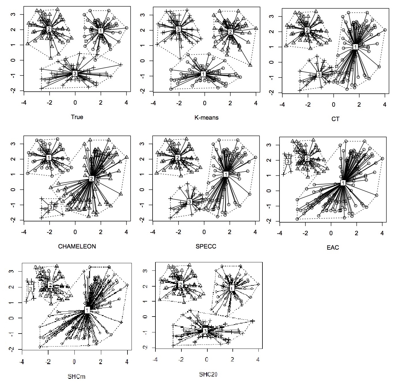
Figure 2: The true clustering of one run of 3-NORMALS data and seven estimated clusterings using K-m, CT, CHA, SPECC, EAC, SHCm, and SHC20.

These observations are mostly but not thoroughly consistent with Table 1 in which MAI values are rounded to two decimal places and SAI values are rounded to three decimal places. Table 1 is the summary of the performance of the six methods over 200 simulated data sets; CHA is omitted as noted earlier. Clearly, despite Fig. 2, CT and EAC are poor in an average sense (MAI) while SCHm is comparable to SHC20 – suggesting the single example of SHCm in Fig. 2 is unrepresentative of its general performance. The performance of spectral clustering is better than Fig. 2 suggests but not as good as $K$-means which is best as expected. Loosely, K-m, SPECC. and the two SHC techniques seem to be broadly equivalent. Note that, usually, the size of the SAI values are higher for poorer performing clustering techniques. This can be taken as an assessment of the quality of the clustering.

Table 1: The comparison of the proposed methods on 3-NORMALS data

	method
	K-m	CT	SPECC	EAC	SHCm	SHC20
MAI	.97	0.87	0.94	0.84	0.92	0.93
SAI	0.000	0.031	0.114	0.158	0.126	0.118

4.2 Non-convex examples

Here we compare all seven clustering techniques for the AGGREGATION, SPIRAL, HALF-RING, and FLAME data sets.

4.2.1 AGGREGATION data

The AGGREGATION data, depicted in the top panel of Figure 3, is used in [13] to show the performance of ensembling.

If $K_{T}=7$ is used, the clusterings from the best three methods (CHAMELEON, EAC, and SHC20) are shown in the lower panels of Fig. 3. It is seen that EAC is a little worse than CHAMELEON, and SHC20 because it merges clusters to form cluster 2 and divides a cluster to give clusters 5 and 6. CHAMELEON, being graph theoretic, is better at separating the two clusters while SHC20 includes randomness and therefore separates the two clusters slightly differently over different runs. EAC also includes randomness so the panels in Fig. 3 merely show one run. The result of SHCm is also shown and is noticably worse: SHCm merges two clusters inappropriately and splits another cluster inappropriately into three clusters. This is the only case among the examples here in which SHCm and SCH20 give meaningfully different results, apparently because of the extreme points in the upper left cluster; note that assumption 4) in Theorem 1 is violated.

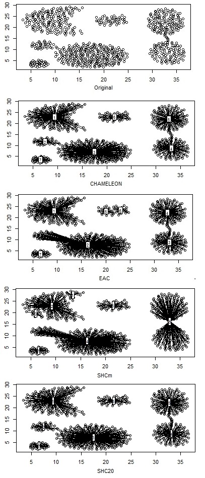
Figure 3: Top panel: Original AGGREGATION data. Second panel: Clustering under CHAMELEON. Third panel: Clustering under EAC. Fourth and fifth panels: Clustering under SHCm and SHC20 respectively

.

These general appearances are consistent with the results in Table 2. Note that CT and CHAMELEON have SAI zero because they are one-pass methods. The overall inference is that SHC20 and CHAMELEON are essentially equivalent in this example.

Table 2: The comparison of the proposed methods on AGGREGATION data

	method
	K-m	CT	SPECC	CHA	EAC	SHCm	SHC20
MAI	0.83	0.81	0.92	1	0.95	0.84	0.98
SAI	0.000	0	0.044	0	0.000	0.000	0.044

4.2.2 SPIRAL data

Figure 4 shows the SPIRAL data that are often considered as a test case for nonconvex clustering. Clearly, $K_{T}=3$ and the clusters are the three lines of points. In this run, only EAC, SHCm and SHC20 find the correct clusters. More generally, if one uses many runs, the MAI and SAI present a slightly different result: The best methods are SPECC and the two SHC’s. Of these, SHC20 and SHCm should be preferred because SPECC has a higher SAI, as can be seen in Table 3.

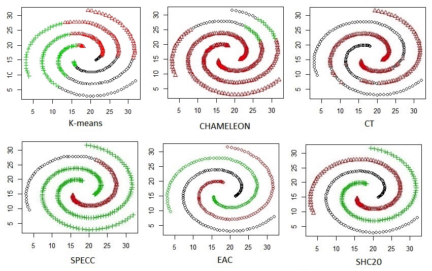
Figure 4: Clustering of the SPIRAL data with six different methods as indicated on the panels; SHCm and SCH20 are idnetical so only SHC20 is shown.

Table 3: The comparison of the proposed methods on SPIRAL data

	method
	K-m	CT	CHA	SPECC	EAC	SHCm	SHC20
MAI	0.34	0.35	0.44	0.94	0.90	1	1
SAI	0.000	0	0	0.148	0.134	0.000	0.000

4.2.3 HALF-RING data

Figure 5 shows six clusterings of the HALF-RING data, considered in [14] (SHCm and SHC20 are nearly identical). Intuitively, there are two clusters but the density of the points makes it ambiguous whether the top half-ring should be split into two clusters or not. It can be seen that K-m and CT give poor performance (they merge the left half of the bottom half ring to the top half ring) but the other methods find the two clusters; this is seen in the results in Table 4. Note that when SHCm and SHC20 are essentialy the same, we only show one of them.

While SHCm and SHC20 have slightly lower MAI’s than the other three good methods (CHAMELEON, SPECC and EAC) they also have nonzero SAI’s indicating the ambiguity in the top half-ring. Indeed, when we ran SHC20 1000 times on the HALF-RING data, the two half rings were in separate clusters 873 times while the right hand portion of the top half-ring was put in the same cluster as the bottom ring 127 times. The ambiguity of two versus three clusters being appropriate is recognized by the SHC’s whereas the SAI’s of the other three good methods (CHAMELEON, SPECC and EAC) being zero indicates they are not recognizing the ambiguity.

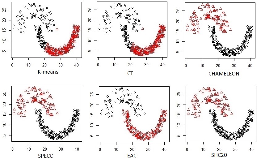
Figure 5: Clustering of the HALF-RING data with six different methods as indicated on the panels; SHCm is the same as SHC20.

Table 4: The comparison of the proposed methods on HALF-RING data

	method
	K-m	CT	CHA	SPECC	EAC	SHCm	SHC20
MAI	0.78	0.78	1	1	1	0.99	0.97
SAI	0	0	0	0	0	0.044	0.063

4.2.4 FLAME data

Fu and Medico [15] developed a fuzzy clustering technique for DNA micro-array wich they considered on the test data given in Figure 6. The website [9] refers to this as the FLAME data set. On this data set, SHCm and SHC20 are seen to be the methods that best identify the two clusters. None of the other five methods do as well; CHAMELEON, EAC, and SPECC fail completely because they are greatly distorted by the two apparent outliers. By contrast, SHCm and SHC20 deal elaborately with outliers to reduce their effect. K-m and CT do passably well, but put too many points in the upper cluster.

The overall performance of the methods is summarized in Table 5 indicating high MAI and relatively low SAI consistent with Fig. 6.

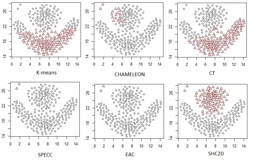
Figure 6: Clustering of FLAME data with six different methods as indicated on the panels (SHCm and SHC20 are identical).

Table 5: The comparison of the proposed methods on FLAME data

	method
	K-m	CT	CHA	SPECC	EAC	SHCm	SHC20
MAI	0.84	0.84	0.71	0.7	0.65	0.89	0.88
SAI	0.031	0	0	0.122	0.0000	0.000	0.000

4.3 Higher dimensional data

In this context it is difficult to generate two or three dimensional plots to evaluate how successful a clustering strategy is visually. One can use projections onto planes, however, doing this systematically increases in difficulty as the dimension increases. Hence, we only present tables of MAI and SAI values. As a generality, CHA can only be expected to work well when the clusters are compact and can be separated; this is less and less likely as dimension increases and the cases when it does occur tend to be those where $K$-means performs well and is easier to use.

4.3.1 IRIS data

This benchmark data set contains $n=$150 observations with three attributes of Iris flowers. Table 6 gives the MAI’s and SAI’s for the replications of the methods on the IRIS data. Obviously, K-m, CT and the two SHC’s methods provide more accurate clustering than the other methods for this data. This is the only one of our examples where CT works well.

Table 6: The comparison of the proposed method on the IRIS data

	method
	K-m	CT	CHA	SPECC	EAC	SHCm	SHC20
MAI	0.89	0.88	0.73	0.69	0.69	0.89	0.88
SAI	0.000	-	-	0.044	0.000	0.054	0.063

4.3.2 GARBER data

To study the performance of the SHC’s with high dimensional data, we used the microarray data from [17]. The data are the 916-dimensional gene expression profiles for lung tissue from $n=72$ subjects. Of these, five subjects were normal and 67 had lung tumors. The classification of the tumors into 6 classes (plus normal) was done by a pathologist giving seven classes total. Accordingly, we expect seven clusters. The data set was constructed in [17] by filling in missing values estimated by the means within the same gene profiles. Table 7 presents the results.

Table 7: The comparison of the proposed method on the GARBER data

	method
data	K-m	CT	CHA	SPECC	EAC	SHCm	SHC20
MAI	0.70	0.63	0.54	0.71	0.80	0.82	0.82
SAI	0.109	-	-	0.054	0.000	0.000	0.000

4.3.3 WINE QUALITY data

The WINE QUALITY data is used in Cortez et al. [16] to study the classification of wines. For red wines, $n=4898$ and seven clusters were found. For white wine, $n=1599$ and 6 clusters were found. Both data sets (for red and white wine) have 11 attributes. Since the data sets are large, we drew $n=300$ observations randomly from each of them. Table 8 gives the MAI’s and SAI’s we found. In both cases, the best methods were the two SHC’s and EAC with the SHC’s being slightly better. The other three methods were worse and even EAC and the SHC’s could not be said to perform well except in a relative sense.

Note that we omitted CHA from this example since it was difficult to use and, as was seen, CHA did poorly on the first two of these higher dimensional examples and K-m was included. We also omitted CT in this example since it never did well (except on the IRIS data, where three other methods did as well).

Table 8: The comparison of the proposed method on the WINE QUALITY data

red wine
	methods
data	K-m	SPECC	EAC	SHCm	SHC20
MAI	0.29	0.4	0.48	0.47	0.48
SAI	0.031	0.070	0.028	0.031	0.031
white wine
	methods
data	K-means	SPECC	EAC	SHCm	SHC20
MAI	0.31	0.38	0.44	0.46	0.46
SAI	0.031	0.0547	0.002	0.044	0.031

4.3.4 Summary of the examples

From these examples, it is seen that CT rarely performs well (only on IRIS) and so can be neglected. CHA works well only on two examples, HALF-RING and AGGREGATION, and its performance is never meaningfully better than both SHC’s. Likewise, SPECC and EAC are never meaningfully better than both SHC’s. Finally, K-m only performs really well on 3-NORMALS, a setting for which it was designed (and even there has close competitors like SHC20 and SPECC), and IRIS (although only trivially). The inference from this is that, as a generality, one of SHCm and SHC20 is the best method. The only meaningful difference in our examples occurred for AGGREGATION where SHC20 outperformed SHCm. Thus, although our theoretical results support SHCm, we are led to SHC20 as a default.

4.4 Estimating cluster size

Estimating the number of clusters is challenging because it requires knowing the structure of the underlying population something that is often not known. That is, identifying the number of groups in a data set is a problem that is both physically and mathematically challenging. Nevertheless, there are several methods to estimate the number of clusters, $\widehat{K}_{T}$. For instance, [18] uses the gap statistic (gap) and it is implemented in the cluster package in R. Another popular method is the Silhouette distance (sil), [1], implemented in the fpc package in R. In addition, one can estimate $K_{T}$ using the Bayesian information criterion (BIC), intializing by a hierarchical clustering as in implemented, for instance, in mclust in R, see [19].

Table 9 shows the estimates of the number of clusters and the true number of clusters using six different methods for the data sets in the previous sub-sections. The numbers in parentheses are the standard deviations (SD’s) for the estimates. The bottom row is the absolute error (AE) formed by taking the sum of the absolute differences between the true and the estimated number of clusters. A simple glance at the results shows that if the raw numbers are rounded to their nearest integers then even though the EK methods based on SHCm and SHC20 do not always identify the correct number of clusters, all other methods perform worse (for the data sets considered). Indeed, gap statistic, sil, and BIC do noticably worse. Only EAC is comparable, and it is slightly worse than EKm which is slightly worse than EK20, again validating our recommendation of using the 20th percentile, i.e., EK20, as a good default. Unfortunately, the SD’s do not seem to provide a helpful guide as to which methods are good; poor methods can have small SD’s and better methods can have larger SD’s unlike for the clustering methods.

Table 9: Estimated numbers of clusters and their SD’s using six techniques.

		methods
data set	actual	EKm	EK20	EAC	Gap	Sil	BIC
FLAME	2	2.2(0.3)	2.1(0.2)	2.1(0.3)	2.7(0.8)	4(0.0)	4(0.0)
SPIRAL	3	3(0.0)	3(0.0)	2.7(1.0)	7.9(1.4)	2(0)	6(0.0)
HALF-RING	2	2.1(0.3)	2.0( 0.1)	2.0(0.4)	1(0)	20(0)	20(0.0)
AGGREGATION	7	5(0)	5(0)	5(0)	2.3(1)	4(0)	10(0)
3-NORMAL	3	3.4(1.7)	3.4(1.6)	3.3(2.3)	2.4(0.9)	3.1(0.3)	3.1(0.4)
IRIS	3	3.0(0.0)	2.9(0.2)	2.0(0.3)	3.4(1.3)	2(0)	2(0)
Red wine	6	3.2(1.6)	3.2(1.7)	3.6(3.8)	8.5(2.8)	2(0)	12.0(3.0)
White wine	7	3.5(2)	3.8(2.1)	3.8(2.8)	10.9(4.4)	2.4(1.3)	12.4(4.0)
GARBER	6	4.2(1.5)	4.6(2.2)	12(10.9)	5.7(2.5)	2(0)	5(0)
AE		10.8	10	15.3	19	35.7	39.5

5 Conclusion

Our approach leads to two natural techniques that differ in the dis-similarity used in the single linkage step of our clustering approach. One dis-similiarity is the usual Euclidean distance between two points. The other is the 20-th percentile of the distances between points in two different clusters. We can establish formal results for the Euclidean distance and it has a naural geometric interpretation. However, the 20-th percentile dissimilarity gives performance that is no worse and sometimes meaningfully better than the Euclidean distance.

In order to evalaute the performance of the proposed methods, we tested them on a wide variety of qualitatively different clusterings, including both real and simulated data, convex and nonconvex true clusterings, and clusterings in which the components are not well separated. Our theory and examples suggest that our methods lead to accurate clusterings and that using $B\approx 250$ to form the membership matrices is enough to provide satisfactory stability. Of course, for more complicated data – irregular shapes, little separation between shapes, etc. – more ensembling (higher $B$) may lead to better results.

In our examples, our methods effectively equal or outperform many standard or related methods such as spectral clustering, $K$-means, EAC [4], hybrid hierachical clustering [5], and CHAMELEON [6]. In fact, in all eight examples we presented here, one of the two forms of our approach always yielded robust and relatively accurate results.

References

- [1] L. Kaufman and P.J. Rousseeuw, Finding groups in data: an introduction to cluster analysis John Wiley & Sons, 2009.
- [2] R. O. Duda, P. E. Hart and D.G. Stork, Pattern classification, John Wiley & Sons, 2012.
- [3] C.C. Aggarwal and C.K. Reddy (Eds.). Data Clustering: Algorithms and Applications, CRC Press, 2013.
- [4] A.L. Fred and A.K. Jain, ”Combining multiple clusterings using evidence accumulation”, IEEE Trans. on Pattern Analysis and Machine Intelligence, 27, 835-850, 2005.
- [5] H. Chipman and R. Tibshirani, ”Hybrid hierarchical clustering with applications to microarray data”, Biostatistics, 7, 286-301, 2006.
- [6] G. Karypis, E.H. Han and V. Kumar, ”Chameleon: Hierarchical clustering using dynamic modeling”. Computer, 32, 68-75, 1999.
- [7] S. Zhong and J. Ghosh, ”A unified framework for model-based clustering”, JMLR, 4, 1001-1037, 2003.
- [8] U. Von Luxburg, ”A tutorial on spectral clustering”, Statistics and computing, 17, 395-416, 2007. 1425-1470, 2010.
- [9] http://cs.joensuu.fi/sipu/datasets/
- [10] https://archive.ics.uci.edu/ml/index.html
- [11] http://genome-www.stanford.edu/lung_cancer/adeno/
- [12] C. Fraley, A. E. Raftery, T. B. Murphy and L. Scrucca, ”mclust Version 4 for R: Normal Mixture Modeling for Model-Based Clustering, Classification, and Density Estimation”, Technical Report No. 597, Department of Statistics, University of Washington, 2012.
- [13] A. Gionis, H. Mannila and P. Tsaparas, Clustering aggregation. ACM Transactions on Knowledge Discovery from Data, 1, 1-30, 2007.
- [14] A.K. Jain and M.H. Law, ”Data clustering: A user’s dilemma.” In: Pattern Recognition and Machine Intelligence, 1-10, Springer, Berlin, 2005.
- [15] L. Fu and E. Medico, ”FLAME, a novel fuzzy clustering method for the analysis of DNA microarray data”, BMC bioinformatics, 8, 2007.
- [16] P. Cortez, A. Cerdeira, F. Almeida, T. Matos and J. Reis. ”Modeling wine preferences by data mining from physicochemical properties”, In: Decision Support Systems, 47, 547-553, 2009.
- [17] M.E. Garber et al., ”Diversity of gene expression in adenocarcinoma of the lung”, PNAS, 98, 13784-13789, 2001.
- [18] R. Tibshirani, G. Walther and T. Hastie, ”Estimating the number of data clusters via the Gap statistic”, J. Roy. Statist. Soc. Ser. B, 63, 411-423, 2001.
- [19] C. Fraley and A.E. Raftery, ”Model-based methods of classification: using the mclust software in chemometrics”. J. Stat. Software, 18, 1-13, 2007.
- [20] Y. Fang and J. Wang, ”Selection of the number of clusters via the bootstrap”, Comp. Stat. and Data Anal., 56, 468-477, 2010.
- [21] A.K. Jain, ”Data clustering: 50 years beyond K-means.” Pattern Recognition Letters, 31, 651-666, 2010.
- [22] M. Meila and D. Heckerman, ”An Experimental Comparison of Several Clustering and Initialization Methods”, Mach. Learn., 42, 9-29, 2001.
- [23] D. Pollard, ”Strong Consistency of K-Means Clustering”, Ann. Statist., 9, 135-140, 1981.