An algebraic multigrid method for quadratic finite element equations of elliptic and saddle point systems in 3D

Abstract.

In this work, we propose a robust and easily implemented algebraic multigrid method as a stand-alone solver or a preconditioner in Krylov subspace methods for solving either symmetric and positive definite or saddle point linear systems of equations arising from the finite element discretization of the vector Laplacian problem, linear elasticity problem in pure displacement and mixed displacement-pressure form, and Stokes problem in mixed velocity-pressure form in 3D, respectively. We use hierarchical quadratic basis functions to construct the finite element spaces. A new heuristic algebraic coarsening strategy is introduced for construction of the hierarchical coarse system matrices. We focus on numerical study of the mesh-independence robustness of the algebraic multigrid and the algebraic multigrid preconditioned Krylov subspace methods.

1. Introduction

Compared to the geometrical multigrid (GMG) method (see, .e.g., [9]), the algebraic multigrid (AMG) method (see, e.g., [21, 18]) is a purely matrix-based approach, that does not rely on any underlying mesh hierarchy; see, e.g., [8] for the development from GMG to AMG methods. Concerning comparison of different types of AMG methods we refer to, e.g., [22] for a review and related references. In contrast to coarsening based on the strongly connected matrix entries in the classical AMG method, an AMG method (among others) with special coarsening and interpolation strategies was introduced in [11], that is based on graph connectivity of the matrix only and leads to fast construction of matrices on coarse levels. An AMG method that is based on the matrix graph information only was also studied early in [3]. The further development of such an AMG method [11] in different applications have been reported in, e.g., [13, 25, 26, 12, 14, 29]. In this work, we focus on the development of such an AMG method for both elliptic and saddle point systems of equations arising from the quadratic finite element discretization for the three dimensional (3D) vector Laplacian problem, linear elasticity problem in pure displacement and mixed displacement-pressure form, and the Stokes problem in mixed velocity-pressure form. This requires new coarsening strategies to construct the hierarchy of matrices on coarse levels for both the elliptic and saddle point systems, that are to be developed in this work. We notice, that different AMG methods towards higher-order finite element equations for second order elliptic problems were also studied using different approaches in, e.g., [20, 16]. The main focus of this work is the numerical study of the robustness and efficiency of the designed AMG method as a stand-alone solver or a preconditioner in Krylov subspace methods for solving the elliptic and saddle point systems.

The remainder of this paper is organized in the following way. In Section 2, we describe the model problems, their finite element discretizations and the arising linear systems of equations. The algebraic multigrid method using a new heuristic coarsening strategy is prescribed in Section 3. In Section 4, we present numerical results of the AMG method applied to discrete model problems. Finally, some conclusions are drawn in Section 5.

2. Preliminaries

2.1. The model problems

Let $\Omega\subset\mathbb{R}^{3}$ be a simply connected and bounded domain with two boundaries $\Gamma_{N}$ and $\Gamma_{D}$ such that $\bar{\Gamma}_{D}\cup\bar{\Gamma}_{N}=\partial\Omega$ and $\Gamma_{N}\cap\Gamma_{D}=\emptyset$. We consider the 3D vector Laplacian problem, the linear elasticity problem in pure displacement and mixed displacement-pressure forms, and the Stokes problem in mixed velocity-pressure form, that are formulated in the following:

For the vector Laplacian problem: Find the potential $u:\bar{\Omega}\mapsto\mathbb{R}^{3}$ such that

(1) $$-\Delta u=0{\textup{ in }}\Omega$$

with the boundary conditions $u=g_{D}$ on $\Gamma_{D}$ and $\frac{\partial u}{\partial n}=g_{N}$ on $\Gamma_{N}$, where $n$ denotes the outward normal vector on $\Gamma_{N}$.

For the linear elasticity problem in pure displacement form: Find the displacement $u:\bar{\Omega}\mapsto\mathbb{R}^{3}$ such that

(2) $$-\nabla\cdot\sigma(u)=0{\textup{ in }}\Omega$$

with the boundary conditions $u=g_{D}$ on $\Gamma_{D}$ and $\sigma(u)n=g_{N}$ on $\Gamma_{N}$. In particular, we use the linear Saint Venant-Krichoff elasticity model. The Cauchy stress tensor and the infinitesimal strain tensor are defined by $\sigma(u)=2\mu\varepsilon(u)+\lambda\text{div}(u)I$ and $\varepsilon(u)=(\nabla u+\nabla u^{T})/2$, respectively, with Lamé constants $\lambda$ and $\mu$.

For the linear elasticity problem in mixed displacement-pressure form: Find the displacement $u:\bar{\Omega}\mapsto\mathbb{R}^{3}$ and pressure $p:\bar{\Omega}\mapsto\mathbb{R}$ such that

(3) $$-\nabla\cdot(2\mu\varepsilon(u))+\nabla p=0 {\textup{ in }}\Omega$$

$$-\nabla\cdot u-\frac{1}{\lambda}p=0 {\textup{ in }}\Omega$$

with the boundary conditions $u=g_{D}$ on $\Gamma_{D}$ and $(2\mu\varepsilon(u)-pI)n=g_{N}$ on $\Gamma_{N}$. It is easy to see that, in this classical mixed displacement-pressure form, the displacement and pressure are associated by the relation $p=-\lambda\nabla\cdot u$; see, e.g., [4].

For the Stokes problem in mixed velocity-pressure form: Find the velocity $u:\bar{\Omega}\mapsto\mathbb{R}^{3}$ and pressure $p:\bar{\Omega}\mapsto\mathbb{R}$ such that

(4) $$-\nabla\cdot(2\mu\varepsilon(u))+\nabla p=0 {\textup{ in }}\Omega$$

$$-\nabla\cdot u=0 {\textup{ in }}\Omega$$

with the boundary conditions $u=g_{D}$ on $\Gamma_{D}$ and $(2\mu\varepsilon(u)-pI)n=g_{N}$ on $\Gamma_{N}$, where $\mu$ denotes the dynamic viscosity.

2.2. The variational formulations

We search for weak solutions of the above four model problems (1)-(4) in proper spaces. For this, let $H^{1}(\Omega)$ and $Q=L^{2}(\Omega)$ denote the standard Sobolev and Lebesgue spaces on $\Omega$; see [1]. With $V={H^{1}(\Omega)}^{3}$, we define the spaces $V_{g}=\{u\in V:u|_{\Gamma_{D}}=g_{D}\}$ for the potential and displacement (velocity) functions. We also define the homogenized space $V_{0}=\{u\in V:u|_{\Gamma_{D}}=0\}$. In addition, we assume the given data $g_{D}\in{H^{1/2}(\Gamma_{D})}^{3}$, where ${H^{1/2}(\Gamma_{D})}^{3}$ denotes the trace space, i.e., ${H^{1/2}(\Gamma_{D})}^{3}=\{v|_{\Gamma_{D}}:v\in H^{1}(\Omega)^{3}\}$. We also assume the given data $g_{N}\in L^{2}(\Gamma_{N})^{3}$. By standard techniques, the following variational formulations are obtained.

The variational formulation for the vector Laplacian problem (1) and the linear elasticity problem (2) in pure displacement form reads (after homogenization): Find $u\in V_{0}$ such that

(5) $$a(u,v)=\langle F,v\rangle$$

for all $v\in V_{0}$, with the bilinear form $a(u,v):=\int_{\Omega}\nabla u:\nabla vdx$ for the vector Laplacian problem and $a(u,v):=\int_{\Omega}[2\mu\varepsilon(u):\varepsilon(v)+\lambda\nabla\cdot u\nabla\cdot v]dx$ for the linear elasticity problem, respectively, and the linear form $\langle F,v\rangle:=\int_{\Gamma_{N}}g_{N}\cdot vdx-a(g_{D},v)$, accordingly.

The variational formulation for the linear elasticity problem (3) in mixed displacement-pressure form and the Stokes problem (4) in mixed velocity-pressure form reads (after homogenization): Find $u\in V_{0}$ and $p\in Q$ such that

(6) $$a(u,v)+b(v,p)=\langle F,v\rangle,$$

$$b(u,q)-c(p,q)=\langle G,q\rangle$$

for all $v\in V_{0}$ and $q\in Q$, where the bilinear and linear forms are given by $a(u,v)=2\mu\int_{\Omega}\varepsilon(u):\varepsilon(v)dx$, $b(v,q)=-\int_{\Omega}q\nabla\cdot vdx$, $\langle F,v\rangle=\int_{\Gamma_{N}}g_{N}\cdot vdx-a(g_{D},v)$, $\langle G,q\rangle=0$ , respectively, and $c(p,q)=\frac{1}{\lambda}\int_{\Omega}pqdx$ and $c(p,q)=0$ for the linear elasticity and Stokes problem, respectively.

2.3. The finite element discretization

The spatial discretization is done by the Galerkin finite element method with a hierarchical quadratic polynomial basis functions. Let ${\mathcal{T}}_{h}$ be the admissible subdivision of the domain $\Omega$ into tetrahedra. The four linear basis functions on each tetrahedron $T\in{\mathcal{T}}_{h}$ are nothing but standard $P_{1}$ hat functions in 3D, i.e., $\phi_{i}:=\lambda_{i}$, $i=1,...,4$, where $\lambda_{i}$ are the barycentric coordinates of $T$. The six quadratic basis functions are then defined as

$$\phi_{5}=4\lambda_{1}\lambda_{2},\;\phi_{6}=4\lambda_{2}\lambda_{3},\;\phi_{7}=4\lambda_{3}\lambda_{4},\;$$

$$\phi_{8}=4\lambda_{1}\lambda_{3},\;\phi_{9}=4\lambda_{1}\lambda_{4},\;\phi_{10}=4\lambda_{2}\lambda_{4},\;$$

that construct hierarchical quadratic polynomial basis functions.

Let $V_{L}:=\{v\in C_{0}(\bar{\Omega}):v_{T}\in\Phi_{T},\forall T\in{\mathcal{T}}_{h}\}$ be the subspace of continuous piecewise linear hat functions with zero traces on $\Gamma_{D}$ and $V_{Q}:=\{v\in C_{0}(\bar{\Omega}):v_{T}\in\Psi_{T},\forall T\in{\mathcal{T}}_{h}\}$ the subspace of continuous piecewise quadratic functions with zero traces on $\Gamma_{D}$, where $\Phi_{T}=\text{span}\{\phi_{i=1,...,4}:T\in{\mathcal{T}}_{h}\}$ and $\Psi_{T}=\text{span}\{\phi_{i=5,...,10}:T\in{\mathcal{T}}_{h}\}$. Let $Q_{L}:=\{v\in C(\bar{\Omega}):v_{T}\in\Phi_{T},\forall T\in{\mathcal{T}}_{h}\}$ be the subspace of continuous piecewise linear hat functions. It can be shown that the global degrees of freedom (DOF) of $V_{L}$, $V_{Q}$, $Q_{L}$ are the number of vertices ($l$) and edges ($m$) (excluding the vertices and edges on $\Gamma_{D}$), and the number of all vertices ($n$), respectively. The global basis functions $\varphi_{i}\in V_{L},Q_{L}$ and $\psi_{i}\in V_{Q}$ can be constructed from the local ones. The function space for one component of the potential or displacement is defined as $V_{h}=V_{L}\oplus V_{Q}\subset V_{0}$, a linear subspace complemented by a quadratic subspace. The function space for the pressure is defined as $Q_{h}=Q_{L}\subset Q$.

Using Galerkin’s principle the discrete elliptic variational formulation for the vector Laplacian and linear elasticity problem in pure displacement form read: Find $u_{h}\in V_{h}$ such that

(7) $$a(u_{h},v_{h})=\langle F,v_{h}\rangle$$

for all $v_{h}\in V_{h}$.

The discrete mixed variational formulation for the elasticity problem in mixed displacement-pressure form and the Stokes problem in mixed velocity-pressure form reads: Find $(u_{h},p_{h})\in V_{h}\times Q_{h}$ such that

(8) $$a(u_{h},v_{h})+b(v_{h},p_{h})=\langle F,v_{h}\rangle,$$

$$b(u_{h},q_{h})-c(p_{h},q_{h})=\langle G,q_{h}\rangle$$

for all $v_{h}\in V_{h}$ and $q_{h}\in Q_{h}$.

The finite element solutions $u_{h}\in V_{h}$ and $p_{h}\in Q_{h}$ are expressed by the ansatz:

$$u_{h}=u_{h}^{l}+u_{h}^{q}=\displaystyle\sum_{i=1}^{l}u_{i}^{l}\varphi_{i}+\displaystyle\sum_{i=1}^{m}u_{i}^{q}\psi_{i},\quad p_{h}=\displaystyle\sum_{i=1}^{n}p_{i}^{l}\varphi_{i},$$

respectively, where $u_{i}^{l},u_{i}^{q}\in\mathbb{R}^{3}$ and $p_{i}^{l}\in\mathbb{R}$. It is easy to see the finite element solution $u_{h}$ is the sum of the linear and quadratic part, $u_{h}^{l}$ and $u_{h}^{q}$, respectively. For the pressure $p_{h}$, we have a linear approximation. The mixed finite element for the elasticity and Stokes problem is classical Taylor-Hood element, that fulfills the $\inf-\sup$ stability requirement; see, e.g., [6].

2.4. SPD and saddle point linear systems of equations

Using the finite element discretization (including homogenization), we obtain the following symmetric and positive definite (SPD) system of equations for the elliptic problem:

(9) $$Au=\left[\begin{array}[]{cc}K_{ll}&K_{ql}^{T}\\ K_{ql}&K_{qq}\\ \end{array}\right]\left[\begin{array}[]{c}\underline{u}_{l}\\ \underline{u}_{q}\end{array}\right]=\left[\begin{array}[]{c}\underline{f}_{l}\\ \underline{f}_{q}\end{array}\right]=f,$$

where $K_{ll}=(a(\varphi_{i},\varphi_{j}))$, $K_{ql}=a(\varphi_{j},\psi_{i})$, $K_{qq}=a(\psi_{i},\psi_{j})$, $\underline{u}_{l}=(u_{i}^{l})$, $\underline{u}_{q}=(u_{i}^{q})$, $\underline{f}_{l}=(\langle F,\varphi_{i}\rangle)$ and $\underline{f}_{q}=(\langle F,\psi_{i}\rangle)$.

For the elasticity problem in mixed displacement-pressure form and the Stokes problem in mixed velocity-pressure form, we obtain the following symmetric indefinite system of equations:

(10) $$\underbrace{\left[\begin{array}[]{cc}A&B^{T}\\ B&-C\end{array}\right]}_{=:K}\left[\begin{array}[]{c}u\\ p\end{array}\right]=\left[\begin{array}[]{cc|c}K_{ll}&K_{ql}^{T}&B^{T}_{ll}\\ K_{ql}&K_{qq}&B^{T}_{lq}\\ \hline\cr B_{ll}&B_{lq}&-C_{ll}\end{array}\right]\left[\begin{array}[]{c}\underline{u}_{l}\\ \underline{u}_{q}\\ \hline\cr\underline{p}_{l}\end{array}\right]=\left[\begin{array}[]{c}\underline{f}_{l}\\ \underline{f}_{q}\\ \hline\cr\underline{g}_{l}\end{array}\right]=\left[\begin{array}[]{c}f\\ g\end{array}\right]$$

where $K_{ll}=(a(\varphi_{i},\varphi_{j}))$, $K_{ql}=a(\varphi_{j},\psi_{i})$, $K_{qq}=a(\psi_{i},\psi_{j})$, $B_{ll}=b(\varphi_{i},\varphi_{j})$, $B_{lq}=b(\varphi_{i},\psi_{j})$, $C_{ll}=c(\varphi_{i},\varphi_{h})$, $\underline{u}_{l}=(u_{i}^{l})$, $\underline{u}_{q}=(u_{i}^{q})$, $\underline{p}_{l}=(p_{i}^{l})$, $\underline{f}_{l}=(\langle F,\varphi_{i}\rangle)$, $\underline{f}_{q}=(\langle F,\psi_{i}\rangle)$ and $\underline{g}_{l}=(\langle G,\varphi_{i}\rangle)$. It is obvious that for the Stokes problem, $C=0$.

In the following, we focus on how to solve the above two systems of equations (9) and (10) using an algebraic multigrid method.

3. An algebraic multigrid method

3.1. The basic algebraic multigrid iteration

The basic AMG iteration applied to a general linear system of equations $Kx=b$ is given in Algorithm 1, with $m_{pre}$ and $m_{post}$ being the number of pre- and post-smoothing steps (steps 1-3 and 14-16, respectively). By choosing $\nu=1$ and $\nu=2$, the iterations in Algorithm 1 are called V- and W-cycle, respectively. As a convention, we use $l=0,...,L$ to indicate the algebraic multigrid levels from the finest level $l=0$ to the coarsest level $l=L$. On the coarsest level $L$, the system is solved by any direct solver (step 6). The coarse grid correction step is indicated in steps 4-13. The full AMG iterations are realized by repeated application of this algorithm. The iteration in this algorithm is also combined with the Krylov subspace methods, that usually leads to accelerated convergence of V-cycle or W-cycle preconditioned methods [22].

Algorithm 1 Basic AMG iteration: AMG($K_{l},x_{l},b_{l}$)

1:  for $k=1$ to $m_{pre}$ do

2:     $x_{l}^{k+1}={\mathcal{S}}_{l}(x_{l}^{k},b_{l})$

3:  end for

4:  $b_{l+1}=R_{l}^{l+1}(b_{l}-K_{l}x_{l})$,

5:  if l+1=L then

6:     Solve $K_{L}x_{L}=b_{L}$

7:  else

8:      $x_{l+1}=0$,

9:     for $k=1,...,\nu$ do

10:        $x_{l+1}=$AMG($K_{l+1},x_{l+1},b_{l+1}$),

11:     end for

12:  end if

13:  $x_{l}=x_{l}+P_{l+1}^{l}x_{l+1}$,

14:  for $k=1$ to $m_{post}$ do

15:     $x_{l}^{k+1}={\mathcal{S}}_{l}(x_{l}^{k},b_{l})$,

16:  end for

17:  return $x_{l}$.

3.2. A new heuristic coarsening strategy

3.2.1. Case I : The SPD system

A robust coarsening strategy is an important feature of the AMG method, that is used to construct the system matrices on coarse levels $l=1,2,...,L$. For the second order elliptic equations discretized by low order finite element or boundary element methods, some well known graph-based black-box or grey-box type AMG methods have been introduced and applied, see, e.g., [3, 11, 17, 13, 12]. The general strategy is to split the nodes into the sets of coarse and fine nodes, based on the graph connectivity of the system matrix or the constructed auxiliary matrix (”virtual” finite element mesh [17]).

When applying such a technique to the system matrix in (9), we obtain a very dense graph connectivity constructed from the stiffness matrix $A$, that contains connectivities for the linear DOF, the quadratic DOF and the coupling between them. This will lead to a mixture of different oder of DOF and may cause additional difficulty to construct the interpolation operators. In fact, from our numerical studies, we observe the loss of optimality of the AMG method when such a dense graph connectivity is adopted for coarse system matrix construction. Therefore, we construct the graph connectivities only for the linear and quadratic DOF, i.e., for $K_{ll}$ and $K_{qq}$, respectively. We simply neglect the coupling connectivity in $K_{ql}$. By this means, we avoid the mixture of different order of DOF on the coarse level. In addition, we are able to construct and control the interpolation operators for the linear and quadratic part, respectively. A simple comparison of the classical and new graph connectivities is illustrated in Fig. 1.

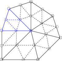
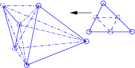
Figure 1. Graph connectivity constructed using the new (left) and the classical (right) strategies: linear DOF (solid line) , quadratic DOF (dashed line) , coupling (dashed dot lines).

From the left plot in Fig. 1, we show the two graph connectivities indicated by solid and dashed lines for the linear and quadratic DOF, respectively. For a comparison, on the right plot, the graph connectivities constructed by the new strategy is reconstructed by the classical strategy. For simplicity, we only reconstruct the part indicated by the lines with blue color. It is easy to obverse that, the classical one leads to much denser graph connectivities than the new one due to the coupling.

Based on these two graph connectivities, the prolongation matrix $P_{l+1}^{l}$ from the coarse level $l+1$ to the next finer level $l$ is constructed in form of

(11) $$P_{l+1}^{l}=\left[\begin{array}[]{cc}I_{l+1}^{l}&\\ &J_{l+1}^{l}\\ \end{array}\right],$$

where the prolongation matrices, $I_{l+1}^{l}:({\mathbb{R}^{3}})^{n_{l+1}}\rightarrow({\mathbb{R}}^{3})^{n_{l}}$ and $J_{l+1}^{l}:({\mathbb{R}^{3}})^{m_{l+1}}\rightarrow({\mathbb{R}}^{3})^{m_{l}}$ are defined for the linear and quadratic DOF, respectively, where $n_{l}$ and $m_{l}$ denote the number of linear and quadratic DOF on level $l$, respectively. The restriction matrix from the finer level $l$ to the next coarser level $l+1$ is constructed as $(P_{l+1}^{l})^{T}$. The system matrix $A_{l+1}$ on the level $l+1$ is constructed by the Galerkin projection method:

$$A_{l+1}=(P_{l+1}^{l})^{T}A_{l}P_{l+1}^{l}.$$

We mention that the two graph connectivities for the linear and quadratic DOF are naturally different as illustrated in Fig. 1. that may require different coarse and fine nodes selection algorithms. However, for simplicity, we apply the coarse and fine nodes selection and prolongation operator matrix construction algorithms developed in [11] for both the linear and quadratic DOF, that show the robustness from the numerical studies.

3.2.2. Case II : The saddle point system

A robust coarsening strategy for saddle point problems is, in general, more involved than that for elliptic problems mainly due to the $\inf-\sup$ instability issues possibly caused by standard Galerkin projection method. For saddle point problems arising from the low order finite element discretized fluid problem, the stability issue has been studied in, e.g., [26, 25, 15]. In [24, 25], a so-called 2-shift coarsening strategy was introduced for the discrete fluid problem using the modified Taylor-Hood element ($P_{1}$iso$P_{2}-P_{1}$), that mimics the hierarchy of matrices in the geometrical multigrid method. To guarantee the $\inf-\sup$ stability for the coarse system is still a research topic.

We extend the new coarsening strategy described above for the elliptic problem, to the saddle point problem, based on the new graph connectivity construction. As illustrated in Fig. 2, we show the graph connectivities constructed for the velocity (displacement) and pressure. For the velocity, we follow the same strategy as for the SPD system; see the left plot. For the pressure, we have conventional graph connectivity for the linear finite element matrix; see the right plot.

Figure 2. Graph connectivities constructed using the new strategies for velocity (displacement) (left) and pressure (right).

Based on the graph connectivities, the prolongation matrix $P_{l+1}^{l}$ from the coarse level $l+1$ to the next finer level $l$ is constructed in form of

(12) $$P_{l+1}^{l}=\left[\begin{array}[]{ccc}I_{l+1}^{l}&&\\ &J_{l+1}^{l}&\\ &&H_{l+1}^{l}\end{array}\right],$$

where the prolongation matrices, $I_{l+1}^{l}:({\mathbb{R}^{3}})^{n_{l+1}}\rightarrow({\mathbb{R}}^{3})^{n_{l}}$ and $J_{l+1}^{l}:({\mathbb{R}^{3}})^{m_{l+1}}\rightarrow({\mathbb{R}}^{3})^{m_{l}}$ are defined for the linear and quadratic velocity DOF, respectively, where $n_{l}$ and $m_{l}$ denote the number of linear and quadratic velocity DOF on level $l$, respectively, $H_{l+1}^{l}:{\mathbb{R}}^{k_{l+1}}\rightarrow{\mathbb{R}}^{k_{l}}$ for the pressure DOF, where $k_{l}$ the number of pressure DOF on level $l$. The restriction matrix from the finer level $l$ to the next coarser level $l+1$ is constructed as $(P_{l+1}^{l})^{T}$. The system matrix $K_{l+1}$ on the level $l+1$ is constructed by the Galerkin projection method:

$$K_{l+1}=(P_{l+1}^{l})^{T}K_{l}P_{l+1}^{l}.$$

We admit that the $\inf-\sup$ stability of the coarse system is still open by this construction. However, from the numerical studies, we observe quite satisfactory results using this new coarsening strategy. Nevertheless, we are at least able to obtain efficient multigrid preconditioners by using pure Galerkin projection; see comments in, e.g., [21, 27] and numerical experiments for the Stokes problem using the low order finite element discretization in, e.g., [10].

3.3. The smoothing procedure

To complete the algebraic multigrid algorithm, a smoothing procedure is needed. As conventional choices, we employ the damped block Jacobi and block Gauss-Seidel smoothers for the SPD system (9), that are widely used in the multigrid methods. For the saddle point system (10), we have considered the following smoothers, that were originally designed and analyzed in the GMG method.

3.3.1. The multiplicative Vanka smoother

The multiplicative Vanka smoother was introduced in [23] for the fluid problem. We have recently developed an AMG method with this smoother for solving the nonlinear and nearly incompressible hyperelastic models in fluid-structure interaction simulation [14]. To adapt this smoother for the Taylor-Hood element, we first construct the patches ${\mathcal{P}}_{i}$, $i=1,...,n$. Each patch contains one pressure DOF, and the connected linear and quadratic velocity DOF indicated by the connectivity of matrices $B_{ll}$ and $B_{lq}$, respectively. A typical patch ${\mathcal{P}}_{i}$ is illustrated in Fig. 3.

Figure 3. A typical local patch ${\mathcal{P}}_{i}$ for the Taylor-Hood element contains one pressure DOF, and connected linear and quadratic velocity DOF.

The local (correction) problem on ${\mathcal{P}}_{i}$ is extracted by a canonical projection of the global one (10) to local one on ${\mathcal{P}}_{i}$:

(13) $$\left[\begin{array}[]{c}u_{i}^{k+1}\\ p_{i}^{k+1}\end{array}\right]=\left[\begin{array}[]{c}u_{i}^{k}\\ p_{i}^{k}\end{array}\right]+\omega\left[\begin{array}[]{cc}A_{i}&B_{i}^{T}\\ B_{i}&-C_{i}\end{array}\right]^{-1}\left[\begin{array}[]{c}r_{u,i}^{k}\\ r_{p,i}^{k}\end{array}\right]$$

with $k$ representing the smoothing step and $\omega$ being a damping parameter. Here $[(r_{u,i}^{k})^{T},(r_{p,i}^{k})^{T}]^{T}$ denotes the residual updated in a multiplicative manner. As we observe from the numerical studies, this smoother shows the efficiency and robustness if it is used in the AMG preconditioner but not in the stand-alone AMG solver.

3.3.2. The Braess-Sarazin-type smoother

This smoother was introduced in [5] and approximated in [30], that has been applied to the fluid problem [25, 26], the nearly incompressible elasticity problem [28] and the fluid-structure interaction problem [29]. One smoothing step corresponds to a preconditioned Richardson method:

(14) $$\left[\begin{array}[]{c}u^{k+1}\\ p^{k+1}\end{array}\right]=\left[\begin{array}[]{c}u^{k}\\ p^{k}\end{array}\right]+\hat{K}^{-1}\left[\begin{array}[]{c}f-Au^{k}-B^{T}p^{k}\\ g-Bu^{k}+Cp^{k}\end{array}\right]$$

with preconditioner

(15) $$\hat{K}=\left[\begin{array}[]{cc}\hat{A}&B^{T}\\ B&B\hat{A}^{-1}B^{T}-\hat{S}\end{array}\right].$$

As in [24], we use $\hat{A}=2D$, where $D$ represents the diagonal of $A$. We use an AMG preconditioner $\hat{S}$ for the approximated Schur complement $C+B\hat{A}^{-1}B$.

3.3.3. The segregated Gauss-Seidel smoother

This smoother was very recently introduced in [7] as a segregated Gauss-Seidel smoother based on a Uzawa-type iteration. Such a Uzawa method (see, e.g., [2]) can be reinterpreted as a preconditioned Richardson method:

(16) $$\left[\begin{array}[]{c}u^{k+1}\\ p^{k+1}\end{array}\right]=\left[\begin{array}[]{c}u^{k}\\ p^{k}\end{array}\right]+\hat{K}^{-1}\left[\begin{array}[]{c}f-Au^{k}-B^{T}p^{k}\\ g-Bu^{k}+Cp^{k}\end{array}\right]$$

with the preconditioner

(17) $$\hat{K}=\left[\begin{array}[]{cc}\hat{A}&\\ B&-\omega^{-1}I\end{array}\right],$$

where $\omega$ is a properly chosen parameter, $\hat{A}$ is a (e.g., AMG) preconditioner for $A$. However, to get a multigrid smoother, this is relaxed by choosing some proper smoother $M_{A}$ for $A$ instead of a preconditioner $\hat{A}$; see [7]. The theoretical analysis requirement for $M_{A}$ has been specified therein. In our setting, we have chosen $M_{A}$ as a damped block Jacobi smoother with a damping parameter $0.5$. Compared to the Braess-Sarazin-type smoother, this smoother avoids the explicite construction of the approximate Schur complement.

4. Numerical results

4.1. Meshes, boundary conditions and coarsening for the vector Laplacian and linear elasticity problems

We consider a unit cube $(0,1)^{3}$ as the computational domain for the vector Laplacian and linear elasticity problems. The domain is subdivided into tetrahedra with four levels of mesh refinement $L_{1}-L_{4}$. The number of tetrahedron (#Tet), nodes (#Nodes) and midside nodes (#Midside nodes), and the total number of DOF for elliptic ( #DOF (elliptic) ) and saddle point ((#DOF (saddle point)) systems are shown in Table 1.

Level	$L_{1}$	$L_{2}$	$L_{3}$	$L_{4}$
#Tet	$64$	$512$	$4096$	$32768$
#Nodes	$125$	$729$	$4913$	$35937$
#Midside nodes	$604$	$4184$	$31024$	$238688$
#DOF (elliptic)	$2187$	$14739$	$107811$	$823875$
#DOF (saddle point)	$2312$	$15468$	$112724$	$859812$

Table 1. Number of tetrahedron (#Tet) , nodes (#Nodes), Midside nodes (#Midside nodes), and total number of DOF for elliptic ( #DOF (elliptic) ) and saddle point (#DOF (saddle point)) systems on four levels $L_{1}-L_{4}$.

We fix the bottom of the domain, i.e., $u=[0,0,0]^{T}$ at $z=0$, prescribe a Dirichlet data on the top, i.e., $u=[0,0,1]^{T}$ at $z=1$, and use zero Neumann condition on the rest of the boundaries. For the linear elasticity problem, we set $\mu=1.15e+06$ and $\lambda=1.73e+06$. In Fig. 4, we plot the value of $\|u\|_{{\mathbb{R}}^{3}}$ of the numerical solution $u$ (indicated by the color) for the vector Laplacian (left) and the linear elasticity problem in pure displacement form (right), respectively. For visualization purpose, we plot the vector fields of potential and deformation, that is scaled by a factor of $0.1$.

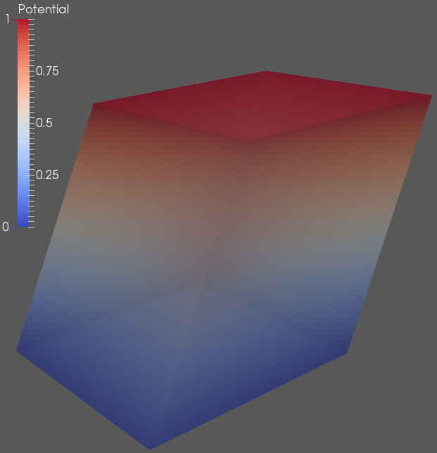
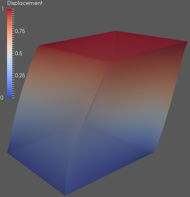
Figure 4. Numerical results of the vector Laplacian (left) and linear elasticity (right) problem.

As a comparison, on each algebraically coarsening level, we show the number of linear and quadratic DOF (# Linear DOF and # Quadratic DOF, respectively) in the new coarsening strategy, and the classical coarsening strategy (# Non-separating DOF); see in Table 2 the number of DOF on each coarsening level for the vector Laplacian and linear elasticity problem on the level $L_{4}$. It is obvious to see these two strategies lead to different graph connectivity in the coarsening procedure.

Coarsening Levels	$0$	$1$	$2$	$3$	$4$
#Linear DOF	$107811$	$14739$	$2187$	$375$	$81$
#Quadratic DOF	$716064$	$104544$	$6366$	$369$	$39$
#Non-separating DOF	$823875$	$88467$	$2187$	$375$	$24$

Table 2. Number of linear and quadratic DOF in the new coarsening strategy, and the total DOF in the non-separating coarsening strategy at level $L_{4}$, for the vector Laplacian and linear elasticity problems.

4.2. Numerical performance for the vector Laplacian problem

Before showing the AMG performance with the new coarsening strategy, we demonstrate the performance with a black-box type AMG [11] in Table 3 for the vector Laplacian problem, where non-separating coarsening strategy is used. For both AMG and AMG preconditioned CG methods, we use the relative residual error $\|f-Au_{k}\|_{l_{2}}/\|f-Au_{0}\|_{l_{2}}=1.0e-11$ in the $l_{2}-$norm as stopping criteria, where $k$ denotes the number of AMG iterations. In each iteration of the AMG solver, we use $2$ W-cycles and $1$ pre- and post-smoothing step. As observed, the AMG and the AMG preconditioned CG are not robust with respect to the mesh refinement, i.e., the iteration number increases with mesh refinement.

Levels	$L_{1}$	$L_{2}$	$L_{3}$	$L_{4}$
#It AMG	$90$	$158$	$>200$	$>200$
#It PCG_AMG	$22$	$25$	$36$	$64$

Table 3. Performance of black-box type AMG solver (#It AMG) and AMG preconditioned conjugate gradient solver (#It PCG_AMG) for the vector Laplacian problem.

Now we show the performance of the AMG and AMG preconditioned CG solvers using the new coarsening strategy. Note, that in the following numerical tests, we stop the iterations when the relative residual error in the $l_{2}-$norm is reduced by a factor $10^{11}$. We consider the Jacobi smoother with damping parameter $0.5$ and $1$ or $2$ pre- and post-smoothing steps (JA-1-1-0.5 or JA-2-2-0.5), and the Gauss-Seidel smoother with $1$ or $2$ pre- and post-smoothing steps (GS-1-1 or GS-2-2). In Table 4, we show the performance of the AMG solver for the vector Laplacian problem using V-cycle with different smoothers. In Table 5, we show the performance using W-cycle. In Table 6 and 7, we show the performance of the AMG preconditioned CG using V- and W-cycles with different smoothers, respectively.

As observed, the iterations for each solver are independent of mesh refinement levels. The AMG solver using the Gauss-Seidel smoother shows better performance than the damped Jacobi smoother. By using the CG acceleration, we observe similar performance with two different smoothers. In addition, we observe, that the V- and W-cycles demonstrate almost the same performance. We also observe that the computational cost is proportional to the number of DOF.

Level	$L_{1}$	$L_{2}$	$L_{3}$	$L_{4}$
#It ( JA-1-1-0.5 )	$129$	$125$	$124$	$128$
#It ( JA-2-2-0.5 )	$65$	$65$	$65$	$66$
#It ( GS-1-1 )	$43$	$46$	$47$	$47$
#It ( GS-2-2 )	$23$	$24$	$24$	$24$

Table 4. Performance of the AMG solver for the vector Laplacian problem using V-cycle with different smoothers.

Level	$L_{1}$	$L_{2}$	$L_{3}$	$L_{4}$
#It ( JA-1-1-0.5 )	$128$	$124$	$121$	$123$
#It ( JA-2-2-0.5 )	$65$	$64$	$63$	$64$
#It ( GS-1-1 )	$43$	$46$	$47$	$47$
#It ( GS-2-2 )	$23$	$24$	$24$	$24$

Table 5. Performance of the AMG solver for the vector Laplacian problem using W-cycle with different smoothers.

Level	$L_{1}$	$L_{2}$	$L_{3}$	$L_{4}$
#It ( JA-1-1-0.5 )	$30$	$30$	$30$	$30$
#It ( JA-2-2-0.5 )	$21$	$22$	$22$	$22$
#It ( GS-1-1 )	$26$	$29$	$29$	$30$
#It ( GS-2-2 )	$17$	$19$	$19$	$19$

Table 6. Performance of the AMG preconditioned CG solver for the vector Laplacian problem using V-cycle with different smoothers.

Level	$L_{1}$	$L_{2}$	$L_{3}$	$L_{4}$
#It ( JA-1-1-0.5 )	$30$	$30$	$30$	$29$
#It ( JA-2-2-0.5 )	$21$	$21$	$21$	$21$
#It ( GS-1-1 )	$26$	$29$	$29$	$29$
#It ( GS-2-2 )	$17$	$18$	$18$	$18$

Table 7. Performance of the AMG preconditioned CG solver for the vector Laplacian problem using W-cycle with different smoothers.

4.3. Numerical performance for the linear elasticity problem in pure displacement form

We perform the same test for the linear elasticity problem. In Table 8, we show the performance of the AMG solver for the linear elasticity problem using V-cycle with different smoothers. In Table 9, we show the performance using W-cycle. In Table 10 and 11, we show the performance of the AMG preconditioned CG using V- and W-cycles with different smoothers, respectively.

As observed, the damped Jacobi smoother does not work for this test problem. The AMG solver using the Gauss-Seidel smoother shows good performance. By using the CG acceleration, we observe improved performance. We observe, that the V- and W-cycles demonstrate almost the same performance.

Level	$L_{1}$	$L_{2}$	$L_{3}$	$L_{4}$
#It ( JA-1-1-0.5 )	$-$	$-$	$-$	$-$
#It ( JA-2-2-0.5 )	$-$	$-$	$-$	$-$
#It ( GS-1-1 )	$80$	$78$	$76$	$75$
#It ( GS-2-2 )	$44$	$40$	$39$	$39$

Table 8. Performance of the AMG solver for the linear elasticity problem in pure displacement form using V-cycle with different smoothers..

Level	$L_{1}$	$L_{2}$	$L_{3}$	$L_{4}$
#It ( JA-1-1-0.5 )	$-$	$-$	$-$	$-$
#It ( JA-2-2-0.5 )	$-$	$-$	$-$	$-$
#It ( GS-1-1 )	$80$	$78$	$75$	$73$
#It ( GS-2-2 )	$44$	$40$	$39$	$44$

Table 9. Performance of the AMG solver for the linear elasticity problem in pure displacement form using W-cycle with different smoothers..

Level	$L_{1}$	$L_{2}$	$L_{3}$	$L_{4}$
#It ( JA-1-1-0.5 )	$50$	$81$	$-$	$-$
#It ( JA-2-2-0.5 )	$32$	$63$	$-$	$-$
#It ( GS-1-1 )	$40$	$43$	$43$	$42$
#It ( GS-2-2 )	$28$	$27$	$27$	$27$

Table 10. Performance of the AMG preconditioned CG solver for the linear elasticity problem in pure displacement form using V-cycle with different smoothers.

Level	$L_{1}$	$L_{2}$	$L_{3}$	$L_{4}$
#It ( JA-1-1-0.5 )	$47$	$80$	$-$	$-$
#It ( JA-2-2-0.5 )	$32$	$62$	$-$	$-$
#It ( GS-1-1 )	$39$	$44$	$42$	$41$
#It ( GS-2-2 )	$28$	$27$	$27$	$26$

Table 11. Performance of the AMG preconditioned CG solver for the linear elasticity problem in pure displacement form using W-cycle with different smoothers.

4.4. Numerical performance for linear elasticity problem in mixed form

For the linear elasticity problem in mixed displacement-pressure form, we plot the simulation results of the displacement and pressure on the left and right plots of Fig. 5, respectively.

We set the relative residual error $1.0e-09$ in the corresponding norm as stopping criteria for solving the saddle point system (indefinite) with both the AMG solver and AMG preconditioned GMRES (see [19]) method. We will only consider the V-cyle for the remaining tests.

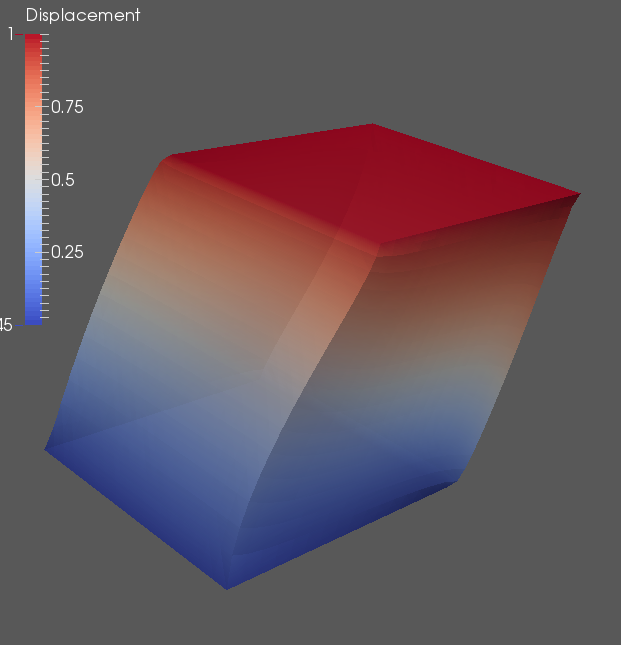
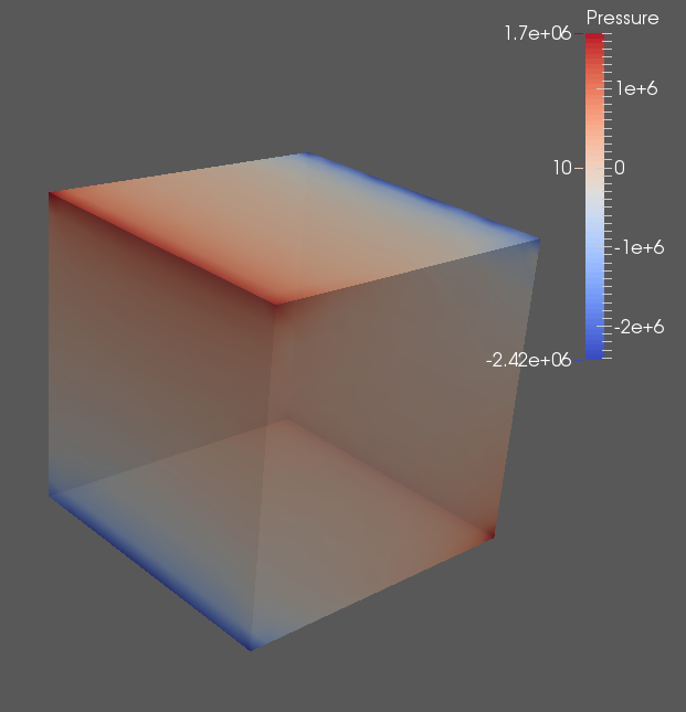
Figure 5. Numerical results of the displacement (left) and pressure (right) for the linear elasticity problem in mixed form.

The AMG solver with the Vanka smoother does not show the robustness and efficiency in this case. However combined with GMRES acceleration, the V-cycle preconditioner with such a smoother shows improved performance. We observe acceptable performance of one or two V-cycles (1 V-cycle or 2 V-cycle) preconditioned GMRES solver in Table 12. In each cycle, we use only one pre- and post-smoothing step.

Level	$L_{1}$	$L_{2}$	$L_{3}$	$L_{4}$
#It ( 1 V-cycle )	$60$	$45$	$49$	$69$
#It ( 2 V-cycles )	$42$	$30$	$32$	$45$

Table 12. Performance of the V-cycle preconditioned GMRES solver for the linear elasticity problem in mixed form using one pre/poster Vanka smoother.

The Braess-Sarazin smoother shows better performance. We observe the robustness with respect to the mesh size of the AMG solver and V-cycle preconditioned GMRES solver using such a smoother; see iteration numbers of the AMG solver using one or two Braess-Sarazin smoothing steps (Braess-Sarazin-1-1 or Braess-Sarazin-2-2) in Table 13, and one or two V-cycles (1 V-cycle or 2 V-cycle) preconditioned GMRES solver in Table 14, respectively.

Level	$L_{1}$	$L_{2}$	$L_{3}$	$L_{4}$
#It ( Braess-Sarazin-1-1 )	$135$	$133$	$125$	$117$
#It ( Braess-Sarazin-2-2 )	$71$	$70$	$66$	$62$

Table 13. Performance of the AMG solver for the linear elasticity problem in mixed form using the V-cycle with the Braess-Sarazin smoother.

Level	$L_{1}$	$L_{2}$	$L_{3}$	$L_{4}$
#It ( 1 V-cycle )	$27$	$27$	$27$	$27$
#It ( 2 V-cycles )	$18$	$19$	$19$	$19$

Table 14. Performance of the V-cycle preconditioned GMRES solver for the linear elasticity problem in mixed form using one pre/post Braess-Sarazin smoother.

Using the segregated Gauss-Seidel smoother (sGS), we observe good performance. For all tests, we use $\omega=0.125$. The robustness with respect to the mesh size of the AMG solver can be observed; see iteration numbers of the AMG solver using one or two segregated Gauss-Seidel smoothing steps (sGS-1-1 or sGS-2-2) in Table 15. The efficiency is further improved when combined with the Krylov subspace acceleration; see iteration numbers of one or two V-cycles (1 V-cycle or 2 V-cycle) preconditioned GMRES solver in Table 16.

Level	$L_{1}$	$L_{2}$	$L_{3}$	$L_{4}$
#It ( sGS-1-1 )	$107$	$104$	$99$	$93$
#It ( sGS-2-2 )	$54$	$53$	$53$	$59$

Table 15. Performance of the AMG solver for the linear elasticity problem in mixed form using the V-cycle with the segregated Gauss-Seidel smoother.

Level	$L_{1}$	$L_{2}$	$L_{3}$	$L_{4}$
#It ( 1 V-cycle )	$14$	$18$	$19$	$21$
#It ( 2 V-cycles )	$12$	$15$	$15$	$15$

Table 16. Performance of the V-cycle preconditioned GMRES solver for the linear elasticity problem in mixed form using one pre/post segregated Gauss-Seidel smoother.

4.5. Numerical performance for the Stokes problem

The computational domain for the Stokes problem is prescribed by an inside of a cylinder, that has radius of $1$ with center point $(0,0,0)$ on the inflow boundary (where $u=(1.0,0,0)$), and center point $(10,0,0)$ on the outflow boundary (where $(2\mu\varepsilon(u)-pI)n=(0,0,0)$). On the rest of the boundaries $u=(0,0,0)$. For all tests, we set $\mu=0.5$. Four levels ($L_{1}-L_{4}$) of tetrahedral meshes are generated; see mesh information for each level in Table 17: The number of tetrahedron (#Tet), nodes (#Nodes) and midside nodes (#Midside nodes), and the total number of DOF ( #DOF ) for the saddle point system. As an illustration to show the coarsening strategy, in Table 18, we show the number of linear and quadratic velocity DOF ( # Linear velocity DOF and # Quadratic velocity DOF) , the linear pressure DOF (# Linear pressure DOF) on each coarsening level for the level $L_{4}$. The velocity and pressure of the simulation results are shown on the left and right plots in Fig. 6, respectively.

Level	$L_{1}$	$L_{2}$	$L_{3}$	$L_{4}$
#Tet	$895$	$7160$	$57280$	$458240$
#Nodes	$351$	$1922$	$12307$	$87109$
#Midside nodes	$1571$	$10385$	$74802$	$566212$
#DOF	$6117$	$38843$	$273634$	$2047072$

Table 17. Fluid mesh information: Number of tetrahedron (#Tet) , nodes (#Nodes) and Midside nodes (#Midside nodes), and the total number of DOF (#DOF) on four levels $L_{1}-L_{4}$.

Coarsening Levels	$0$	$1$	$2$	$3$	$4$
#Linear velocity DOF	$261327$	$36921$	$5766$	$1053$	$267$
#Quadratic velocity DOF	$1698636$	$213492$	$14142$	$1053$	$93$
#Linear pressure DOF	$87109$	$12307$	$1922$	$351$	$89$

Table 18. Number of linear and quadratic velocity, and linear pressure DOF in the new coarsening strategy at level $L_{4}$ for the Stokes problem.

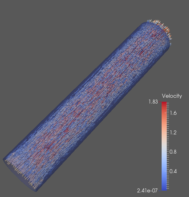
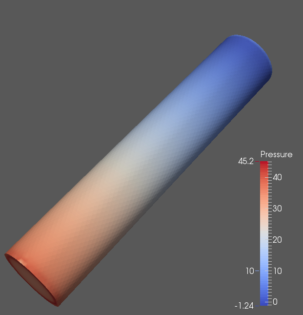
Figure 6. Numerical results of the Stokes velocity (left) and pressure (right).

For this example, the AMG solver with the Vanka, Braess-Sarazin and segregated Gauss-Seidel smoothers shows poor performance, that is very large smoothing steps are required in order to get multigrid convergence rate. However, this will lead to very expensive computational cost. In addition, we observe unsatisfactory performance of the AMG preconditioned Krylov subspace method using the V-cycle with the Vanka and segregated Gauss-Seidel smoothers. Therefore, we only report the performance of the AMG preconditioned GMRES solver using the Braess-Sarazin smoother, that is shown in Table 19. We set relative residual error $1.0e-09$ in the corresponding norm as stopping criteria of the AMG preconditioned GMRES solver. It is easy to see, with the Krylov subspace acceleration, the performance is greatly improved, using one or two V-cycle (1 V-cycle or 2 V-cycle) preconditioner with one pre- and post-smoothing steps.

Level	$L_{1}$	$L_{2}$	$L_{3}$	$L_{4}$
#It ( 1 V-cycle )	$25$	$42$	$38$	$39$
#It ( 2 V-cycles )	$16$	$17$	$18$	$21$

Table 19. Performance of the V-cycle preconditioned GMRES solver for the Stokes problem using one pre/post Braess-Sarazin smoother.

5. Conclusions

In this work, we have developed an AMG method used as a stand-alone solver or preconditioner in the Krylov subspace methods for solving the finite element equations of the vector Laplacian problem, linear elasticity problem in pure displacement and mixed displacement-pressure form, and the Stokes problem in mixed velocity-pressure form in 3D. We have developed a new strategy to construct the hierarchy of the AMG coarsening system using the hierarchical quadratic basis functions. The numerical studies have demonstrated the good performance of the AMG solvers or the AMG preconditioned Krylov subspace methods for the elliptic and saddle point systems, respectively. In particular, the AMG preconditioned Krylov subspace methods show much better robustness and efficiency for solving both systems compared with the AMG stand-alone solvers. From this point of view, the AMG method developed in this work can be used as a robust and efficient solver or preconditioner for the SPD system and the saddle point system with compressible materials, and as a robust and efficient preconditioner for the saddle point system with incompressible materials. It is also possible to extend this AMG method for high-order hierarchical finite element basis functions.

References

- [1] R.A. Adams and J.J.F. Fournier. Sobolev Spaces. Academic Press, Amsterdam, Boston, 2003.
- [2] Michele Benzi, G.H. Golub, and J. Liesen. Numerical solution of saddle point problems. Acta Numerica, 14:1–137, 5 2005.
- [3] D. Braess. Towards algebraic multigrid for elliptic problems of second order. Computing, 55(4):379–393, 1995.
- [4] D. Braess. Finite Elements - Theory, Fast Solvers, and Applications in Solid Mechanics. Cambridge University Press, Cambridge, New York, 2007.
- [5] D. Braess and R. Sarazin. An efficient smoother for the Stokes problem. Appl. Numer. Math., 23(1):3–19, 1997.
- [6] F. Brezzi and M. Fortin. Mixed and Hybrid Finite Element Methods. Springer, New York, 1991.
- [7] F.J. Gaspar, Y. Notay, C.W. Oosterlee, and C. Rodrigo. A simple and efficient segregated smoother for the discrete Stokes equations. SIAM J. Sci. Comput., 36(3):A1187–A1206, 2014.
- [8] G. Haase and U. Langer. Modern Methods in Scientific Computing and Applications, volume 75 of NATO Science Series II. Mathematics, Physics and Chemistry, chapter Multigrid Methods: From Geometrical to Algebraic Versions, pages 103–154. Kluwer Academic Press, Dordrecht, 2002.
- [9] W. Hackbusch. Multi-Grid Methods and Applications. Springer, Heidelberg, 2003.
- [10] A. Janka. Smoothed aggregation multigrid for a Stokes problem. Comput. Visual. Sci., 11(3):169–180, 2008.
- [11] F. Kickinger. Algebraic multigrid for discrete elliptic second-order problems. In Multigrid Methods V. Proceedings of the 5th European Multigrid conference (ed. by W. Hackbush), Lecture Notes in Computational Sciences and Engineering, vol. 3, pages 157–172. Springer, 1998.
- [12] U. Langer and D. Pusch. Data-sparse algebraic multigrid methods for large scale boundary element equations. Appl. Numer. Math., 54(3–4):406–424, 2005.
- [13] U. Langer, D. Pusch, and S. Reitzinger. Efficient preconditioners for boundary element matrices based on grey-box algebraic multigrid methods. Int J Numer Meth Engng, 58(13):1937–1953, 2003.
- [14] U. Langer and H. Yang. Partitioned solution algorithms for fluid-structure interaction problems with hyperelastic models. J. Comput. Appl. Math., 276(0):47–61, 2015.
- [15] B. Metsch. Algebraic Multigrid (AMG) for Saddle Point Systems. PhD thesis, Rheinischen Friedrich-Wihelms-Universität Bonn, 2013.
- [16] A. Napov and Y. Notay. Algebraic multigrid for moderate order finite elements. SIAM J Sci Comput, 2014. to appear.
- [17] S. Reitzinger. Algebraic Multigrid Methods for Large Scale Finite Element Methods. PhD thesis, Johannes Kepler University Linz, 2001.
- [18] J. W. Ruge and K. Stüben. Algebraic multigrid. In S.F. McCormick, editor, Multigrid Methods, volume 3 of Frontiers in Applied Mathematics, pages 73–130. SIAM, Philadelphia, PA, 1987.
- [19] Y. Saad and Martin H. Schultz. GMRES: A generalized minimal residual algorithm for solving nonsymmetric linear systems. SIAM J. Sci. Stat. Comput., 7(3):856–869, 1986.
- [20] S. Shu, D. Sun, and J. Xu. An algebraic multigrid method for higher-order finite element discretizations. Computing, 77(4):347–377, 2006.
- [21] K. Stüben. Multigrid, chapter Appendix A: An introduction to algebraic multigrid, pages 413–533. Academic Press, 2001.
- [22] K. Stüben. A review of algebraic multigrid. J. Comput. Appl. Math., 128(1–2):281–309, 2001.
- [23] S.P. Vanka. Block-implicit multigrid solution of Navier-Stokes equations in primitive variables. J. Comput. Phys., 65(1):138–158, 1986.
- [24] M. Wabro. Algebraic Multigrid Methods for the Numerical Solution of the Incompressible Navier-Stokes Equations. PhD thesis, Johannes Kepler University Linz, 2003.
- [25] M. Wabro. Coupled algebraic multigrid methods for the Oseen problem. Comput Visual Sci, 7(3-4):141–151, 2004.
- [26] M. Wabro. AMGe—coarsening strategies and application to the Oseen equations. SIAM J Sci Comput, 27(6):2077–2097, 2006.
- [27] T. Wiesner. Flexible Aggregration-based Algebraic Multigrid Method for Contact and Flow Problems. PhD thesis, Technischen Universität München, 2015.
- [28] H. Yang. Partitioned solvers for the fluid-structure interaction problems with a nearly incompressible elasticity model. Comput. Visual. Sci., 14(5):227–247, 2011.
- [29] H. Yang and W. Zulehner. Numerical simulation of fluid-structure interaction problems on hybrid meshes with algebraic multigrid methods. J. Comput. Appl. Math., 235(18):5367–5379, 2011.
- [30] W. Zulehner. A class of smoothers for saddle point problems. Computing, 65(3):227–246, 2000.