Probing the Majorana neutrinos and their CP violation in decays of charged scalar mesons $\pi,K,D,D_{s},B,B_{c}$

Abstract

Some of the outstanding questions of particle physics today concern the neutrino sector, in particular whether there are more neutrinos than those already known and whether they are Dirac or Majorana particles. There are different ways to explore these issues. In this article we describe neutrino-mediated decays of charged pseudoscalar mesons such as $\pi^{\pm}$, $K^{\pm}$ and $B^{\pm}$, in scenarios where extra neutrinos are heavy and can be on their mass shell. We discuss semileptonic and leptonic decays of such kinds. We investigate possible ways of using these decays in order to distinguish between the Dirac and Majorana character of neutrinos. Further, we argue that there are significant possibilities of detecting CP violation in such decays when there are at least two almost degenerate Majorana neutrinos involved. This latter type of scenario fits well into the known neutrino minimal standard model ($\nu$MSM) which could simultaneously explain the Dark Matter and Baryon Asymmetry of the Universe.

I Introduction

To date it is unclear whether the neutrinos we know are Dirac of Majorana fermions. Unlike Dirac fermions, Majorana fermions cannot be distinguished from their own antiparticles. As a consequence, processes involving Dirac neutrinos conserve charges such as Lepton Number, while processes involving Majorana neutrinos will not conserve them. There exist several processes which may clarify the Majorana or Dirac nature of neutrinos. Among such processes the most prominent are neutrinoless double beta decays ($0\nu\beta\beta$) in nuclei 0nubb ; 0nubb2 ; 0nubb3 ; 0nubb31 ; 0nubb4 ; 0nubb5 ; 0nubb6 ; 0nubb7 ; 0nubb8 ; 0nubb9 . Other such processes are specific scattering processes  scatt1 ; scatt12 ; scatt13 ; scatt14 ; scatt2 ; scatt3 ; scatt4 ; DevscattLR ; DevscattLR2 ; Devscattssaw ; Devscattssaw1 , and rare meson decays LittSh ; LittSh2 ; DGKS ; Ali ; IvKo ; GoJe ; Atre ; HKS ; QLD ; QLD1 ; QLD2 ; Abada ; Wang ; Boya ; CDKK ; CDK ; CKZ ; CKZ2 ; DCK .

A related issue in neutrinos physics is the absolute mass values of the known neutrinos. While the experimental evidence of neutrino oscillations within the known three flavor states oscatm ; oscsol ; oscsol2 ; oscsol3 ; oscsol4 ; oscnuc clearly shows that these particles cannot all be massless, the oscillations are only sensitive to mass differences, not to their absolute values. In contrast, $0\nu\beta\beta$ decays are sensitive to the absolute mass and may help in their determination, if neutrinos turn out to be Majorana particles. So far the best bounds on the absolute masses of the light neutrinos come from Cosmology $m_{\nu}\gtrsim 0.23$ eV PlanckColl .

A pending question is then why light neutrinos are so light, specifically so much lighter than all other Standard Model (SM) fermions. Interesting enough, the existence of such very light neutrinos can be explained via the seesaw mechanism seesaw ; seesaw2 ; seesaw3 ; seesaw4 ; seesaw5 where more neutrinos are required and where all of them are, in general, Majorana particles. In the simplest form of this mechanism, the masses of the light neutrinos are $\sim{\cal M}_{D}^{2}/{\cal M}_{R}$ ($\lesssim$1 eV), where ${\cal M}_{D}$ is an electroweak scale or lower. At the same time, additional neutrinos, usually much heavier (with masses ${\cal M}_{R}\gg 1$ TeV) and sterile under electroweak interactions except through small mixing with the SM flavors, are required. This mixing is suppressed as $\sim{\cal M}_{D}/{\cal M}_{R}$ ($\ll$1). Besides the simplest scenario, there are other seesaw scenarios in which the heavy neutrinos may have lower masses, namely near or below 1 TeV Wyler1 ; Witten1 ; Mohapatra1 ; Malinsky1 ; Devseesaw ; Devseesaw2 ; Devseesaw3 and even near the 1 GeV scale or below scatt2 ; nuMSM ; nuMSM2 ; HeAAS ; HeAAS2 ; KS ; AMP , and at the same time their mixing with the SM flavors may not be so extremely suppressed as in the original scenarios.

In the first part of this work we discuss lepton number violating (LNV) semileptonic decays of charged pseudoscalar mesons such as $K^{\pm}$ and $B^{\pm}$, mediated by a heavy Majorana neutrino on its mass shell, cf. Ref. CDKK . The pions, which are the lightest mesons, can have only leptonic decays; we discuss hypothetical leptonic decays that could be mediated by on-shell heavy neutrinos. Such decays could be either lepton number conserving (LNC) or lepton number violating (LNV) when the mediating neutrinos are Majorana particles, cf. Ref. CDK , while only LNC decays occur when the neutrino is of Dirac type. We present ways of determining the nature of neutrinos using the differential decay rates of these processes.

Yet another interesting issue in neutrino physics is the possible existence of CP violation in the lepton sector, a phenomenon that could be measured, for example, in neutrino oscillations oscCP . Alternatively, as we present in the second part of this work, leptonic CP violation may show in leptonic LNC and LNV decays of charged pions, cf. Ref. CKZ , or in semileptonic LNV decays of $K^{\pm}$ and $B^{\pm}$, cf. Refs. CKZ2 ; DCK . It turns out that such CP violation becomes appreciable and possibly detectable in these decays if the scenario contains at least two on-shell heavy neutrinos that are almost degenerate. Interestingly, this scenario fits well into the neutrino minimal standard model ($\nu$MSM) nuMSM ; nuMSM2 ; Shapo ; Shapo2 ; Shapo3 ; Shapo4 ; Shapo5 ; Shapo6 which contains two almost degenerate Majorana neutrinos of mass $\sim$ 1 GeV and another lighter neutrino of mass $\sim 10^{1}$ keV, besides the three light neutrinos of mass $\lesssim$1 eV. This model can explain simultaneously the existence of neutrino oscillations, dark matter and baryon asymmetry of the Universe. Furthermore, in more general frameworks of low-scale seesaw, baryon asymmetry (but not dark matter) is explained while keeping even larger values of the heavy-light mixing 1404.7114 than in the $\nu$MSM, and in such frameworks the case of almost degenerate Majorana neutrinos is preferred 1502.00477 since it allows larger mixings. CP violation effects in the neutrino sector in scenarios with nearly degenerate heavy neutrinos have also been investigated earlier Pilaftsis ; Pilaftsis2 using a more detailed formalism, although it amounts to the same effect described here which is the interference of amplitudes with two slightly different dispersive and absorptive parts in the neutrino self energy.

In Section II we discuss the LNV semileptonic decays of mesons $M^{\pm}\to\ell_{1}^{\pm}\ell_{2}^{\pm}M^{\prime\mp}$, mediated by an on-shell Majorana neutrino (which henceforth we call $N$) where $M$ is a heavy pseudoscalar ($M=K,D,D_{s},B,B_{c}$), $M^{{}^{\prime}}$ is a lighter pseudoscalar, and $\ell_{j}$ ($j=1,2$) are charged leptons, and we present there the corresponding branching ratios. In Section III we present the expressions and values of the branching ratios for the LNC and LNV leptonic decays of charged pions mediated by on-shell $N$ sterile neutrino, $\pi^{\pm}\to e^{\pm}N\to e^{\pm}e^{\pm}\mu^{\mp}\nu$, as well as the differential branching ratio $d{\rm Br}/dE_{\mu}$ for these decays. We discuss the possibilities of detecting such branching ratios and to discern from them the Majorana or Dirac nature of neutrinos. In Section IV we then extend the analysis of the mentioned leptonic and semileptonic decays to a scenario where we have at least two heavy on-shell sterile neutrinos involved ($N_{1}$, $N_{2}$), and we present an analysis of CP-violating asymmetries ${\cal A}_{\rm CP}\equiv[\Gamma(M^{-})-\Gamma(M^{+})]/[\Gamma(M^{-})+\Gamma(M^{+})]$ for such processes. In Appendices 1 and 2 we present explicit formulas for our LNV semileptonic decays, and in Appendices 4 and 5 explicit formulas needed for the analysis of our LNC and LNV leptonic decays of the charged pion. Appendix 3 contains formulas needed for evaluation of the decay width of the heavy neutrino $N$, and in Appendix 6 we derive an identity relevant for CP violation asymmetry. In Section V we discuss and summarize our results.

II Lepton Number Violating Semileptonic Decays of Scalar Mesons

If there is a Majorana sterile neutrino $N$ with mass $M_{N}\sim 1$ GeV, its existence could be discerned by detecting semileptonic LNV decays of heavy mesons mediated by on-shell $N$. Here we will consider such LNV decays $M^{\pm}\to\ell_{1}^{\pm}N\to\ell_{1}^{\pm}\ell_{2}^{\pm}M^{{}^{\prime}\mp}$, where $M$ and $M^{{}^{\prime}}$ are pseudoscalar mesons ($M=K,D,D_{s},B,B_{c}$; $M^{{}^{\prime}}=\pi,K,D,D_{s}$) while $\ell_{1}$ and $\ell_{2}$ are charged leptons ($e,\mu$ or $\tau$), cf. Figure 1.

Large part of this Section uses the results of Refs. CDKK ; CDK , and for certain general formulas, those of Refs. CKZ2 ; DCK .

We consider a scenario where we have at least one heavy sterile neutrino $N$, which has (small) mixing $B_{\ell N}$ with the three known neutrino flavors $\nu_{\ell}$ ($\ell=e,\mu,\tau$)

$$\nu_{\ell}=\sum_{k=1}^{3}B_{\ell\nu_{k}}\nu_{k}+B_{\ell N}N+\ldots\$$ (1)

Here, $\nu_{k}$ ($k=1,2,3$) are the three light mass neutrino eingenstates. The considered decays may be appreciable only if $N$ can go on its mass shell (in the $s$-type channel, Figure 1), creating a very large resonant enhancement of order $m_{N}/\Gamma_{N}$, condition which is fulfilled if

$$(M_{M^{\prime}}+M_{\ell_{2}}) < M_{N}<(M_{M}-M_{\ell_{1}})\ ,\ {\rm or/and}$$

$$(M_{M^{\prime}}+M_{\ell_{1}}) < M_{N}<(M_{M}-M_{\ell_{2}})\$$ (2)

Consequently, only tree level resonant amplitudes need to be considered. The mixing matrix $B$ appearing in Equation (1) should be unitary, implying that the PMNS $3\times 3$ block $B_{\ell\nu_{k}}$ ($\ell=e,\mu,\tau$ and $k=1,2,3$) is in general not unitary. If one adds extra and heavy neutrinos—as in most seesaw models—the unitarity of $B$ thus provides upper limit constraints on the heavy-to-light mixing elements Akhmedov ; Abada ; Qian ; Basso . This is in part one of the reasons for the high suppression suffered by all lepton flavour violating processes involving heavy neutrinos.

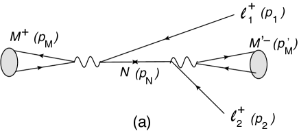
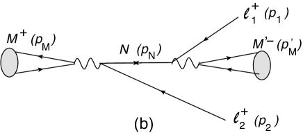
Figure 1: The lepton number violating (LNV) semileptonic decay $M^{+}(p_{M})\to\ell^{+}_{1}(p_{1})\ell^{+}_{2}(p_{2})M^{{}^{\prime}-}(p_{M^{\prime}})$ mediated by a Majorana neutrino $N$: (a) the direct ($D$) channel; (b) the crossed ($C$) channel.

II.1 Branching Ratio for $M^{\pm}\to\ell_{1}^{\pm}\ell_{2}^{\pm}M^{{}^{\prime}\mp}$

The decay width of the considered decays can be written as final particles’ phase space integral of the square of the reduced decay amplitude ${\cal T}(M^{\pm})$ (summed over helicities of charged leptons)

$$\Gamma(M^{\pm}\to\ell_{1}^{\pm}\ell_{2}^{\pm}M^{{}^{\prime}\mp})=(2-\delta_{\ell_{1}\ell_{2}})\frac{1}{2!}\frac{1}{2M_{M}}\frac{1}{(2\pi)^{5}}\int d_{3}\;|{\cal T}(M^{\pm})|^{2}\$$ (3)

Factor $1/2!$ above is the symmetry factor when the two produced leptons are equal; $d_{3}$ is the integration differential of the final three-particle phase space

$$d_{3}\equiv\frac{d^{3}{\vec{p}}_{1}}{2E_{\ell_{1}}({\vec{p}}_{1})}\frac{d^{3}{\vec{p}}_{2}}{2E_{\ell_{2}}({\vec{p}}_{2})}\frac{d^{3}{\vec{p}}_{M^{\prime}}}{2E_{M^{\prime}}({\vec{p}}_{M^{\prime}})}\delta^{(4)}\left(p_{M}-p_{1}-p_{2}-p_{M^{\prime}}\right)\$$ (4)

The resulting decay width can be written as

$$\Gamma(M^{\pm}\to\ell_{1}^{\pm}\ell_{2}^{\pm}M^{{}^{\prime}\mp}) = (2-\delta_{\ell_{1}\ell_{2}})|k|^{2}\left[{\widetilde{\Gamma}}(DD^{*})+{\widetilde{\Gamma}}(CC^{*})+{\widetilde{\Gamma}}_{\pm}(DC^{*})+{\widetilde{\Gamma}}_{\pm}(CD^{*})\right]\$$ (5)

where $k$ is the mixing factor

$$k=B_{\ell_{1}N}B_{\ell_{2}N}\$$ (6)

and ${\widetilde{\Gamma}}_{\pm}(XY^{*})$ are the normalized (i.e., without the explicit mixing) contributions from the $X$ channel and the complex-conjugate of the $Y$ channel ($X,Y=D,C$, where $D$ and $C$ stand for the direct and crossed channels)

$${\widetilde{\Gamma}}_{\pm}(XY^{*})\equiv K^{2}\;\frac{1}{2!}\frac{1}{2M_{M}}\frac{1}{(2\pi)^{5}}\int d_{3}\;P(X)P(Y)^{*}M_{N}^{2}T_{\pm}(X)T_{\pm}(Y)^{*}\$$ (7)

The expressions for $T_{\pm}(X)T_{\pm}(Y)^{*}$ ($X,Y=D,C$) are given in Appendix 1. $T_{\pm}(X)$ is the relevant part of the amplitude in the $X$ channel and forms part of the total decay amplitude ${\cal T}(M^{\pm})$, cf. Appendix 1. In Equation (5), notice that subscripts $\pm$ for the contributions ${\widetilde{\Gamma}}(DD^{*})$ and ${\widetilde{\Gamma}}(CC^{*})$ are unnecessary because $|T_{+}(D)|^{2}=|T_{-}(D)|^{2}$ and $|T_{+}(C)|^{2}=|T_{-}(C)|^{2}$. $P(X)$ ($X=D,C$) are the propagator functions of the intermediate neutrino $N$ in the two channels

$$P(D) = \frac{1}{\left[(p_{M}-p_{1})^{2}-M_{N}^{2}+i\Gamma_{N}M_{N}\right]}\$$ (8a)

$$P(C) = \frac{1}{\left[(p_{M}-p_{2})^{2}-M_{N}^{2}+i\Gamma_{N}M_{N}\right]}\$$ (8b)

The overall constant $K^{2}$ in Equation (7) is

$$K^{2}=G_{F}^{4}f_{M}^{2}f_{M^{\prime}}^{2}|V_{Q_{u}Q_{d}}V_{q_{u}q_{d}}|^{2}\$$ (9)

Here, $f_{M}$ and $f_{M^{\prime}}$ are the decay constants of $M^{\pm}$ and $M^{{}^{\prime}\mp}$, and $V_{Q_{u}Q_{d}}$ and $V_{q_{u}q_{d}}$ are the corresponding CKM matrix elements. We denote the valence quark content of $M^{+}$ as $Q_{u}{\bar{Q}}_{d}$; of $M^{{}^{\prime}+}$ as $q_{u}{\bar{q}}_{d}$.

When the intermediate neutrino $N$ has such a mass that it is on mass shell, Equation (2), the squares of the propagators (8) are reduced to Dirac delta functions because $\Gamma_{N}\ll M_{N}$

$$|P(X)|^{2} = \left|\frac{1}{(p_{M}-p_{k})^{2}-M^{2}_{N}+i\Gamma_{N}M_{N}}\right|^{2}$$ (10)

$$= \frac{\pi}{M_{N}\Gamma_{N}}\delta((p_{M}-p_{k})^{2}-M^{2}_{N})\qquad(\Gamma_{N}\ll M_{N})\$$

where $p_{k}=p_{1},p_{2}$ for $X=D,C$. In this on-shell case, the $DD^{*}$ and $CC^{*}$ contributions in Equation (5) are large, and the interference contributions $DC^{*}$ and $CD^{*}$ are negligible in comparison (cf. Ref. CKZ2 for details on this point), leading to

$$\Gamma(M^{\pm}\to\ell_{1}^{\pm}\ell_{2}^{\pm}M^{{}^{\prime}\mp}) = (2-\delta_{\ell_{1}\ell_{2}})|k|^{2}\left[{\widetilde{\Gamma}}(DD^{*})+{\widetilde{\Gamma}}(CC^{*})\right]$$ (11a)

$$\equiv \Gamma(M^{\pm}\to\ell_{1}^{\pm}\ell_{2}^{\pm}M^{{}^{\prime}\mp};DD^{*})+\Gamma(M^{\pm}\to\ell_{1}^{\pm}\ell_{2}^{\pm}M^{{}^{\prime}\mp};CC^{*})\$$ (11b)

when $\ell_{1}=\ell_{2}$, we even have ${\widetilde{\Gamma}}(DD^{*})={\widetilde{\Gamma}}(CC^{*})$. The normalized decay width ${\widetilde{\Gamma}}(DD^{*})$ can be calculated explicitly, and it turns out to be

$${\widetilde{\Gamma}}(DD^{*}) = \frac{K^{2}M_{M}^{5}}{128\pi^{2}}\frac{M_{N}}{\Gamma_{N}}\lambda^{1/2}(1,y_{N},y_{\ell_{1}})\lambda^{1/2}\left(1,\frac{y^{\prime}}{y_{N}},\frac{y_{\ell_{2}}}{y_{N}}\right)Q(y_{N};y_{\ell_{1}},y_{\ell_{2}},y^{\prime})\$$ (12)

and ${\widetilde{\Gamma}}(CC^{*})$ is obtained by the simple exchange $y_{\ell_{1}}\leftrightarrow y_{\ell_{2}}$

$${\widetilde{\Gamma}}(CC^{*}) = {\widetilde{\Gamma}}(DD^{*})(y_{\ell_{1}}\leftrightarrow y_{\ell_{2}})\$$ (13)

The notations used in Equations (12) and (13) are

$$\lambda(y_{1},y_{2},y_{3}) = y_{1}^{2}+y_{2}^{2}+y_{3}^{2}-2y_{1}y_{2}-2y_{2}y_{3}-2y_{3}y_{1}\$$ (14a)

$$y_{N} = \frac{M_{N}^{2}}{M_{M}^{2}}\ ,\quad y_{\ell_{s}}=\frac{M_{\ell_{s}}^{2}}{M_{M}^{2}}\ ,\quad y^{\prime}=\frac{M_{M^{\prime}}^{2}}{M_{M}^{2}}\ ,\quad(\ell_{s}=\ell_{1},\ell_{2})\$$ (14b)

and the function $Q(y_{N};y_{\ell_{1}},y_{\ell_{2}},y^{\prime})$ is given in Appendix 2. In the limit of massless charged leptons ($y_{\ell_{1}}=y_{\ell_{2}}=0$), the expression (12) reduces to

$${\widetilde{\Gamma}}(DD^{*}){\big{|}}_{M_{\ell_{1}}=M_{\ell_{2}}=0} = \frac{K^{2}M_{M}^{5}}{256\pi^{2}}\frac{M_{N}}{\Gamma_{N}}y_{N}^{2}(1-y_{N})^{2}\left(1-\frac{y^{\prime}}{y_{N}}\right)^{2}$$ (15)

We note that the expression (12), although having the explicit mixing dependence factored out [cf. Equation (11)], contains the dependence on the mixing coefficients $B_{\ell N}$ in the denominator due to the $N$-decay width there $\Gamma_{N}\propto|B_{\ell N}|^{2}$ ($\ell=e,\mu,\tau$, see below). This factor $1/\Gamma_{N}$ in ${\widetilde{\Gamma}}(DD^{*})$ of Equation (12) represents the $N$-on-shell effect Equation (10). As a result, the considered width $\Gamma(M^{\pm}\to\ell_{1}^{\pm}\ell_{2}^{\pm}M^{{}^{\prime}\mp})$ is by many orders of magnitude larger when $N$ is on-shell than it would be if $N$ were off-shell. For more quantitative analyses, it is thus important to have an expression for $\Gamma_{N}$ as a function of mass $M_{N}$. Using the results of Ref. CKZ2 , we can write this decay width as

$$\Gamma_{N}={\widetilde{\cal K}}{\overline{\Gamma}}_{N}(M_{N})\$$ (16)

where the corresponding canonical (i.e., without any mixing dependence) decay width is

$${\overline{\Gamma}}_{N}(M_{N})\equiv\frac{G_{F}^{2}M_{N}^{5}}{96\pi^{3}}\$$ (17)

and the factor ${\widetilde{\cal K}}$ contains the dependence on the heavy-light mixing factors

$${\widetilde{\cal K}}(M_{N})\equiv{\widetilde{\cal K}}={\cal N}_{eN}\;|B_{eN}|^{2}+{\cal N}_{\mu N}\;|B_{\mu N}|^{2}+{\cal N}_{\tau N}\;|B_{\tau N}|^{2}\$$ (18)

In this expression, ${\cal N}_{\ell N}(M_{N})\equiv{\cal N}_{\ell N}$ ($\ell=e,\mu,\tau$) are the effective mixing coefficients; these are numbers $\sim 10^{0}$–$10^{1}$ which depend on the mass $M_{N}$. In Appendix 3 we write down the relevant formulas for the evaluation of these coefficients. The results of these evaluations are presented in Figure 2, for the case of Majorana and Dirac neutrino $N$, in the entire neutrino mass interval $0.1\ {\rm GeV}<M_{N}<6.3\ {\rm GeV}$ which will be of interest in this work. For further clarifying remarks we refer to Appendix 3. Equations (11) and (12) imply that $\Gamma(M^{\pm}\to\ell_{1}^{\pm}\ell_{2}^{\pm}M^{{}^{\prime}\mp})$ is proportional to $1/{\widetilde{\cal K}}$ ($\propto 1/|B_{\ell N}|^{2}$). Hence, we can define a canonical branching ratio ${\overline{\rm Br}}$, being the part of the branching ratio ${\rm Br}(DD^{*})\equiv\Gamma(M^{\pm}\to\ell_{1}^{\pm}\ell_{2}{\pm}M^{{}^{\prime}\mp};DD^{*})/\Gamma(M^{\pm}\to{\rm all})$ with no explicit or implicit heavy-light mixing factors

$${\rm Br}(M^{\pm}\to\ell_{1}^{\pm}\ell_{2}^{\pm}M^{{}^{\prime}\mp};DD^{*}) \equiv \frac{\Gamma(M^{\pm}\to\ell_{1}^{\pm}\ell_{2}^{\pm}M^{{}^{\prime}\mp};DD^{*})}{\Gamma(M^{\pm}\to{\rm all})}=\frac{(2-\delta_{\ell_{1}\ell_{2}})|k|^{2}}{\Gamma(M^{\pm}\to{\rm all})}{\widetilde{\Gamma}}(DD^{*})$$ (19a)

$$= (2-\delta_{\ell_{1}\ell_{2}})\frac{|k|^{2}}{{\widetilde{\cal K}}}2{\overline{\rm Br}}(y_{N};y_{\ell_{1}},y_{\ell_{2}};y^{\prime})\$$ (19b)

Use of the expressions (12) and Equations (16) and (17) then gives for the canonical branching ratio the following expression:

$${\overline{\rm Br}}(DD^{*}) \equiv {\overline{\rm Br}}(y_{N};y_{\ell_{1}},y_{\ell_{2}},y^{\prime})$$ (20)

$$= \frac{3\pi}{8}\frac{K^{2}M_{M}}{G_{F}^{2}\Gamma(M^{\pm}\to{\rm all})}\frac{1}{y_{N}^{2}}\lambda^{1/2}(1,y_{N},y_{\ell_{1}})\lambda^{1/2}\left(1,\frac{y^{\prime}}{y_{N}},\frac{y_{\ell_{2}}}{y_{N}}\right)Q(y_{N};y_{\ell_{1}},y_{\ell_{2}},y^{\prime})\$$

where the notations (14) and (9) are used. In the limit of massless charged leptons ($M_{\ell_{1}}=M_{\ell_{2}}=0$) this expression becomes simpler

$${\overline{\rm Br}}(y_{N};0,0,y^{\prime})=\frac{3\pi}{16}\frac{K^{2}M_{M}}{G_{F}^{2}\Gamma(M^{\pm}\to{\rm all})}(1-y_{N})^{2}\left(1-\frac{y^{\prime}}{y_{N}}\right)^{2}$$ (21)

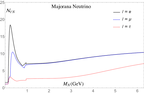
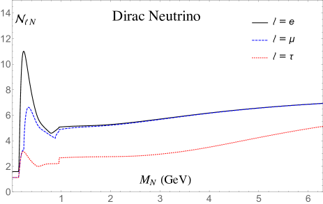
Figure 2: The effective mixing coefficients ${\cal N}_{\ell N}$ ($\ell=e,\mu,\tau$) appearing in Equations (16)–(18), as a function of the mass $M_{N}$ of the neutrino $N$. The left-hand figure is for the case of Majorana neutrino; the right-hand figure for the case of Dirac neutrino. For details we refer to Appendix 3.

II.2 Effect of the Long Neutrino Lifetime on the Observability of $M^{\pm}\to\ell_{1}^{\pm}\ell_{2}^{\pm}M^{{}^{\prime}\mp}$

In the mentioned branching ratios, an often important effect of suppression due to the decay (i.e., nonsurvival) probability was not included. Namely, if the detector for the considered decays has a certain length $L$, the produced (on-shell) massive neutrino $N$ could survive during its flight through the detector, and would decay later outside it. Such decays are thus not detected and should be eliminated from the width and the branching ratio of the considered process $M^{\pm}\to\ell_{1}^{\pm}\ell_{2}^{\pm}M^{{}^{\prime}\mp}$, by introducing a suppression factor (nonsurvival probability) $P_{N}=1-\exp[-t/(\tau_{N}\gamma_{N})]$, where $t\approx L/\beta_{N}$ is the time of flight of $N$ through the detector ($\beta_{N}$ is the velocity of $N$ in the lab frame), and $\gamma_{N}=(1-\beta_{N}^{2})^{-1/2}$ is the Lorentz time dilation factor. Hence, the suppression factor, which should multiply the branching ratio, is

$$P_{N}=1-\exp\left[-\frac{L}{\tau_{N}\gamma_{N}\beta_{N}}\right]\approx 1-\exp\left[-\frac{L\Gamma_{N}}{\gamma_{N}}\right]\$$ (22)

In the last relation, we used $\beta_{N}\approx 1$ and $\tau_{N}=1/\Gamma_{N}$ [$\equiv 1/\Gamma(N\to{\rm all})$], in the units used here ($c=1=\hbar$). This decay-within-the-detector probability $P_{N}$ has been discussed and presented for the processes with intermediate on-shell particle (such as $N$) in Refs. CDK ; scatt3 ; CKZ ; CKZ2 ; CERN-SPS ; CERN-SPS2 ; commKim . In this respect, here we follow mostly the notations of Ref. CKZ2 . Usually, the quantity $P_{N}$ is small and is then written as

$$P_{N}\approx L/(\tau_{N}\gamma_{N}\beta_{N})\quad\left(\approx L/(\tau_{N}\gamma_{N})\right)\qquad{\rm if}\;P_{N}\ll 1$$ (23)

which agrees with Equation (22) in the limit of small $P_{N}$. The suppression factor (22) can be rewritten as

$$P_{N} = 1-\exp\left(-\frac{L}{L_{N}}\right)=1-\exp\left(-\frac{L}{{{\overline{L}}}_{N}}{\widetilde{\cal K}}\right)$$ (24a)

$$\approx \frac{L}{{{\overline{L}}}_{N}}{\widetilde{\cal K}}\quad{\rm if}\;P_{N}\ll 1$$ (24b)

Here, $L_{N}$ is the decay length, and ${{\overline{L}}}_{N}$ is the canonical decay length (independent of the mixing parameters $B_{\ell^{{}^{\prime}}N}$)

$$L_{N}^{-1} = {{\overline{L}}}_{N}^{-1}{\widetilde{\cal K}}\$$ (25a)

$${{\overline{L}}}_{N}^{-1} = \frac{{\overline{\Gamma}}_{N}(M_{N})}{\gamma_{N}}=\frac{1}{\gamma_{N}}\frac{G_{F}^{2}M_{N}^{5}}{96\pi^{3}}\$$ (25b)

where ${\widetilde{\cal K}}$ and ${\overline{\Gamma}}_{N}(M_{N})$ are from Equations (16)–(18), cf. also Figure 2. Equation (24b) suggests that it is convenient to define a canonical (i.e., independent of mixing) probability ${\overline{P}}_{N}$ for the decay of $N$ within the detector as

$${\overline{P}}_{N}=\frac{1{\rm m}}{{{\overline{L}}}_{N}}\;\Rightarrow P_{N}\approx{\overline{P}}_{N}\left(\frac{L}{1{\rm m}}\right){\widetilde{\cal K}}$$ (26)

We present the inverse canonical decay length, ${\overline{L}}_{N}^{-1}$, for $\gamma_{N}=2$, in Figure 3 as a function of $M_{N}$. We note that ${\overline{L}}_{N}^{-1}$ increases very fast (as $M_{N}^{5}$) when $M_{N}$ increases. Therefore, the supression due to the factor $P_{N}$ may not necessarily be strong (i.e., $P_{N}\not\ll 1$) for semileptonic LNV decays of heavier mesons $M^{\pm}$, such as $B^{\pm}$.

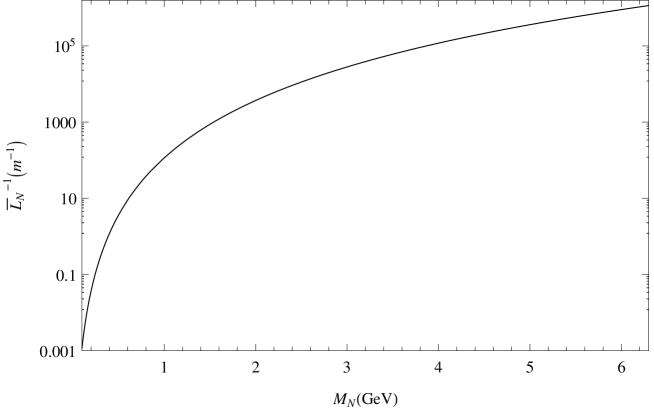
Figure 3: The inverse canonical decay length ${\overline{L}}_{N}^{-1}\equiv{\overline{\Gamma}}_{N}(M_{N})/\gamma_{N}$, Equation (25b), in units of inverse meters ($m^{-1}$), as a function of the neutrino mass $M_{N}$, with the Lorentz lab time dilation factor chosen to be $\gamma_{N}$ [$\equiv(1-\beta_{N}^{2})^{-1/2}$] $=2$. The $y$ axis can also be interpreted as the canonical probability ${\overline{P}}_{N}\equiv(1{\rm m})/{\overline{L}}_{N}$ (dimensionless), Equation (26).

If we use eyeball estimates for the coefficients ${\cal N}_{\ell N}$ of the left-hand Figure 2, approximate expressions for the factor ${\widetilde{\cal K}}$ of Equation (18) for Majorana neutrinos can be written

$${\widetilde{\cal K}} \approx 15|B_{eN_{j}}|^{2}+8|B_{\mu N_{j}}|^{2}+2|B_{\tau N_{j}}|^{2}\quad(K\;{\rm decays})\$$ (27a)

$${\widetilde{\cal K}} \approx 7(|B_{eN_{j}}|^{2}+|B_{\mu N_{j}}|^{2})+2|B_{\tau N_{j}}|^{2}\quad(D,D_{s}\;{\rm decays})\$$ (27b)

$${\widetilde{\cal K}} \approx 8(|B_{eN_{j}}|^{2}+|B_{\mu N_{j}}|^{2})+3|B_{\tau N_{j}}|^{2}\quad(B,B_{c}\;{\rm decays})\$$ (27c)

In order to estimate better the values of ${\widetilde{\cal K}}$ Equations (27) and thus the suppression factor $P_{N}$ Equation (24), we need to know the present upper bounds for the squares $|B_{\ell N}|^{2}$ as a function of $M_{N}^{2}$. These upper bounds we take from compilation of values of Ref. Atre , based in turn on upper bound values obtained in Refs. Benes ; Belanger ; Belanger2 ; Kusenko ; beamdump ; beamdump2 ; beamdump3 ; beamdump4 ; beamdump5 ; l3etal ; l3etal2 ; delphi ; noch ; noch2 . We present them in Table 1, for specific chosen values of $M_{N}$ in the mass range of interest.

Table 1: Presently known upper bounds for the squares $|B_{\ell N}|^{2}$ of the heavy-light mixing matrix elements, for various specific values of $M_{N}$.

$M_{N}[GeV]$	$|B_{eN}|^{2}$	$|B_{\mu N}|^{2}$	$|B_{\tau N}|^{2}$
0.1	$(1.5\pm 0.5)\times 10^{-8}$	$(6.0\pm 0.5)\times 10^{-6}$	$(8.0\pm 0.5)\times 10^{-4}$
0.3	$(2.5\pm 0.5)\times 10^{-9}$	$(3.0\pm 0.5)\times 10^{-9}$	$(1.5\pm 0.5)\times 10^{-1}$
0.5	$(2.0\pm 0.5)\times 10^{-8}$	$(6.5\pm 0.5)\times 10^{-7}$	$(2.5\pm 0.5)\times 10^{-2}$
0.7	$(3.5\pm 0.5)\times 10^{-8}$	$(2.5\pm 0.5)\times 10^{-7}$	$(9.0\pm 0.5)\times 10^{-3}$
1.0	$(4.5\pm 0.5)\times 10^{-8}$	$(1.5\pm 0.5)\times 10^{-7}$	$(3.0\pm 0.5)\times 10^{-3}$
2.0	$(1.0\pm 0.5)\times 10^{-7}$	$(2.5\pm 0.5)\times 10^{-5}$	$(3.0\pm 0.5)\times 10^{-4}$
3.0	$(1.5\pm 0.5)\times 10^{-7}$	$(2.5\pm 0.5)\times 10^{-5}$	$(4.5\pm 0.5)\times 10^{-5}$
4.0	$(2.5\pm 0.5)\times 10^{-7}$	$(1.5\pm 0.5)\times 10^{-5}$	$(1.5\pm 0.5)\times 10^{-5}$
5.0	$(3.0\pm 0.5)\times 10^{-7}$	$(1.5\pm 0.5)\times 10^{-5}$	$(1.5\pm 0.5)\times 10^{-5}$
6.0	$(3.5\pm 0.5)\times 10^{-7}$	$(1.5\pm 0.5)\times 10^{-5}$	$(1.5\pm 0.5)\times 10^{-5}$

Table 2: Rough estimates of upper bounds for $|B_{\ell N}|^{2}$ ($\ell=e,\mu,\tau$), for $M_{N}$ in three different ranges around the values $0.25$, $1$, $3$ GeV; and the inverse of the canonical decay length, ${{\overline{L}}}_{N}^{-1}$ (in units of $m^{-1}$ and for $\gamma_{N}=2$).

$M_{N}$ [GeV]	$|B_{eN}|^{2}$	$|B_{\mu N}|^{2}$	$|B_{\tau N}|^{2}$	${{\overline{L}}}_{N}^{-1}[m^{-1}]$
$\approx 0.25$	$10^{-8}$	$10^{-7}$	$10^{-4}$	0.11
$\approx 1.0$	$10^{-7}$	$10^{-7}$	$10^{-2}$	$1.1\times 10^{2}$
$\approx 3.0$	$10^{-6}$	$10^{-4}$	$10^{-4}$	$3\times 10^{4}$

We remark that the upper bounds have in some cases strong dependence on the precise values of $M_{N}$, see Ref. Atre for further details. In order to use only rough estimates for the values of ${\widetilde{\cal K}}$, we present in Table 2 order of magnitude values for upper bounds of $|B_{\ell N}|^{2}$. These rough upper bounds are given for three typical ranges of our interest: $M_{N}$ around $0.25$; $1$; $3$ GeV. They are relevant for the decays of $K$; ($D,D_{s}$); ($B,B_{c}$), respectively. The corresponding values of the inverse of the canonical decay length, ${{\overline{L}}}_{N}^{-1}$, are included. As seen in Tables 1 and 2, the upper bounds for $|B_{\tau N}|^{2}$ are at present significantly less stringent and are expected to become more stringent in the future. When we combine Equations (24b) with (27) and Table 2, we obtain for the decay-within-the-detector probability $P_{N}\equiv{\overline{P}}_{N}{\widetilde{\cal K}}$ the following estimates and upper bounds, relevant for the $K$ decays ($M_{N}\approx 0.25$ GeV), $D$ and $D_{s}$ decays ($M_{N}\approx 1$ GeV), and $B$ and $B_{c}$ decays ($M_{N}\approx 3$ GeV), all when $L=1$ m and $\gamma_{N}=2$:

$$P_{N}(M_{N}\approx 0.25{\rm GeV}) \approx 1.7|B_{eN_{j}}|^{2}+0.9|B_{\mu N_{j}}|^{2}\quad(+0.2|B_{\tau N_{j}}|^{2})$$ (28a)

$$\lesssim 10^{-8}+10^{-7}\quad(+10^{-5})\$$

$$P_{N}(M_{N}\approx 1{\rm GeV}) \approx 0.8\cdot 10^{3}|B_{eN_{j}}|^{2}+0.8\cdot 10^{3}|B_{\mu N_{j}}|^{2}\quad(+2\cdot 10^{2}|B_{\tau N_{j}}|^{2})$$ (28b)

$$\lesssim 10^{-4}+10^{-4}\quad(+10^{0})\$$

$$P_{N}(M_{N}\approx 3{\rm GeV}) \approx 3\cdot 10^{5}|B_{eN_{j}}|^{2}+3\cdot 10^{5}|B_{\mu N_{j}}|^{2}\quad(+1\cdot 10^{5}|B_{\tau N_{j}}|^{2})$$ (28c)

$$\lesssim 10^{0}+10^{0}\quad(+10^{0})\$$

In order to have the analysis and the formulas simpler, in the rest of this Section we will assume that one mixing parameter, $|B_{\ell N}|$, dominates over the other two mixing parameters:

$$|B_{\ell N}|\gg|B_{\ell^{\prime}N}|\qquad(\ell^{{}^{\prime}}\not=\ell)$$ (29)

For example, it may well be that $\ell=\mu$, i.e., that $|B_{\mu N}|\gg|B_{eN}|,|B_{\tau N}|$. Then, of the branching ratios ${\rm Br}(M^{\pm}\to\ell^{\pm}_{1}\ell^{\pm}_{2}M^{{}^{\prime}\mp})$ the largest will be $M^{\pm}\to\ell^{\pm}\ell^{\pm}M^{{}^{\prime}\mp}$ which, according to Equations (29) and (19) (note that $DD^{*}$ and $CC^{*}$ give the same contribution since $\ell_{1}=\ell_{2}$ now), is:

$${\rm Br}(M^{\pm}\to\ell^{\pm}\ell^{\pm}M^{{}^{\prime}\mp})=4\frac{|B_{\ell N}|^{4}}{{\widetilde{\cal K}}}{\overline{\rm Br}}$$ (30)

Multiplying this expression by the probability $P_{N}$ of the decay in the detector, Equation (26), we obtain the effective branching ratio ${\rm Br}_{\rm eff}$

$${\rm Br}_{\rm eff}(M^{\pm}\to\ell^{\pm}\ell^{\pm}M^{{}^{\prime}\mp}) = P_{N}{\rm Br}(M^{\pm}\to\ell^{\pm}\ell^{\pm}M^{{}^{\prime}\mp})=\left[{\overline{P}}_{N}\left(\frac{L}{1{\rm m}}\right){\widetilde{\cal K}}\right]\times\left[4\frac{|B_{\ell N}|^{4}}{{\widetilde{\cal K}}}{\overline{\rm Br}}\right]$$ (31a)

$$= \left(\frac{L}{1{\rm m}}\right)4|B_{\ell N}|^{4}{\overline{P}}_{N}{\overline{\rm Br}}\equiv|B_{\ell N}|^{4}\left(\frac{L}{1{\rm m}}\right){\overline{\rm Br}}_{\rm eff}$$ (31b)

We see that in the effective branching ratio, ${\rm Br}_{\rm eff}$, the complicated dependence on mixing parameters encoded in ${\widetilde{\cal K}}$ [cf. Equation (18)] disappeared because factors ${\widetilde{\cal K}}$ cancel here. All the mixing effects in ${\rm Br}_{\rm eff}$ are in the simple factor $|B_{\ell N}|^{4}$. Unfortunately, this factor represents a strong suppression, in comparison with ${\rm Br}$ of Equations (19) where ${\rm Br}\propto|k|^{2}/{\widetilde{\cal K}}=|B_{\ell_{1}N}B_{\ell_{2}N}|^{2}/{\widetilde{\cal K}}\sim|B_{\ell N}|^{2}$.

In the last identity (31b) we introduced the canonical (i.e., without any mixing dependence) effective branching ratio ${\overline{\rm Br}}_{\rm eff}$

$${\overline{\rm Br}}_{\rm eff}\equiv 4{\overline{P}}_{N}{\overline{\rm Br}}=4\left(\frac{1{\rm m}}{{{\overline{L}}}_{N}}\right){\overline{\rm Br}}\$$ (32)

where we recall that ${\overline{\rm Br}}$ was defined in Equations (19) and (20). Here $\overline{\rm Br_{eff}}$ is half the value of $\overline{\rm Br_{eff}}$ in Ref. CKZ2 because the latter expression referred to the exchange of two Majorana neutrinos instead of one.

Only when $M^{\pm}=B^{\pm}$ or $B_{c}^{\pm}$, i.e., when the mass of the on-shell $N$ can be high ($M_{N}\gtrsim 1$ GeV), would it be possible to have $P_{N}\sim 1$ [Equation (28c)]; and in such a case Equations (31) do not apply, but rather Equations (30), i.e., ${\rm Br}_{\rm eff}={\rm Br}$ in this case. Figures 4–7 show the effective canonical branching ratios (32) as a function of the neutrino mass $M_{N}$, for various considered LNV decays of the type $M^{\pm}\to\ell^{\pm}\ell^{\pm}M^{{}^{\prime}\mp}$: Figure 4 for $M=K$; Figure 5a, b for $M=D,D_{s}$, respectively; Figures 6a and 7a for $M=B,B_{c}$, respectively. We took $\ell=e,\mu$, and $L=1$ m and $\gamma_{N}=2$. For the case when $P_{N}\sim 1$ and hence the estimates Equations (30) apply, Figures 6b and 7b present the branching ratios ${\overline{\rm Br}}(x)$ as a function of $M_{N}$, for $M^{\pm}=B^{\pm}$ and $B_{c}^{\pm}$, respectively. For the meson decay constants and CKM matrix elements, needed for the evaluation of $K^{2}$ factor of Equation (9), and for the masses and lifetimes of the mesons, we used the values of Ref. PDG2014 . The values of the decay constants $f_{B}$ and $f_{B_{c}}$ were taken from Ref. CKWN : $f_{B}=0.196$ GeV, $f_{B_{c}}=0.322$ GeV. We note that the presented formulas for ${\overline{\rm Br}}_{\rm eff}$ and ${\overline{\rm Br}}$ can be evaluated also for the decays $M^{\pm}\to\ell_{1}^{\pm}\ell_{2}^{\pm}M^{{}^{\prime}\mp}$ when $\ell_{1}\not=\ell_{2}$. Furthermore, when the final leptons are $\tau$ leptons (and $M^{\pm}=B^{\pm}$ or $B_{c}^{\pm}$), the values of branching ratios turn out to be similar to those in Figures 6 and 7, but the range of $M_{N}$ in this case is shorter: $M_{M^{{}^{\prime}}}+M_{\tau}<M_{N}<M_{M}-M_{\tau}$. Table 3 displays values of ${\overline{\rm Br}}_{\rm eff}$ for representative values of $M_{N}$ in the decays $M^{\pm}\to\ell^{\pm}\ell^{\pm}M^{{}^{\prime}\mp}$.

Table 3: Values of the factor ${\overline{\rm Br}}_{\rm eff}$, Equation (32), with $L=1$ m and $\gamma_{N}=2$, for some of the LNV decays $M^{\pm}\to\ell^{\pm}\ell^{\pm}\pi^{\mp}$. The value of $M_{N}$ is chosen such that the maximal value of ${\overline{\rm Br}}_{\rm eff}$ is obtained (the value of $M_{N}$ is given in parentheses, in GeV). For $M^{\pm}=K^{\pm}$, two different values are given, for $\ell=e$ and $\ell=\mu$. For all other cases, $\ell=\mu$ is taken (when $\ell=e$ the values are similar).

$M^{\pm}$:	$K^{\pm}$ ($\ell=e$)	$K^{\pm}$ ($\ell=\mu$)	$D^{\pm}$	$D_{s}^{\pm}$	$B^{\pm}$	$B_{c}^{\pm}$
${\overline{\rm Br}}_{\rm eff}$	6.8 (0.38)	3.8 (0.35)	3.9 (1.39)	70. (1.47)	0.96 (3.9)	199. (4.7)

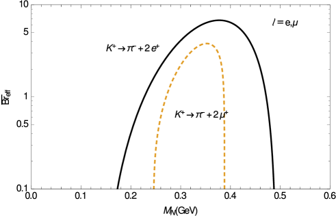
Figure 4: The effective canonical branching ratio (32) for the decays $K^{\pm}\to\ell^{\pm}\ell^{\pm}\pi^{\mp}$ ($\ell=e,\mu$) as a function of the Majorana neutrino mass $M_{N}$.

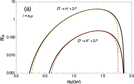
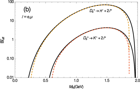
Figure 5: The same as in Figure 4, but now for the decay of (a) $D^{\pm}$ mesons; (b) $D_{s}^{\pm}$ mesons. The solid lines are for $\ell=e$, and the dashed lines for $\ell=\mu$.

Figure 6: (a) The effective canonical branching ratio (32) as a function of $M_{N}$ for the lepton number violating (LNV) decays $B^{\pm}\to\ell^{\pm}\ell^{\pm}M^{{}^{\prime}\mp}$, where $\ell=e,\mu$ (no visible difference between $\ell=e$ and $\ell=\mu$); (b) the theoretical canonical branching ratio ${\overline{\rm Br}}$, Equations (19) and (20), for these decays.

Figure 7: The same as in Figure 6, but for the LNV decays of the charmed mesons $B_{c}^{\pm}$.

As an illustrative example, let us consider the decays $D_{s}^{\pm}\to\mu^{\pm}\mu^{\pm}\pi^{\mp}$, which is one of the preferred decay modes proposed at CERN-SPS CERN-SPS ; CERN-SPS2 , and, in addition, let us assume that $|B_{\mu N}|^{2}$ is the dominant mixing. In such a case, Equations (31) and Table 3 imply for the experimentally measurable branching fraction ${\rm Br}_{\rm eff}$

$${\rm Br}_{\rm eff}(D^{\pm}_{s}\to\mu^{\pm}\mu^{\pm}\pi^{\mp})\equiv P_{N}{\rm Br}(D^{\pm}_{s}\to\mu^{\pm}\mu^{\pm}\pi^{\mp})\sim 10^{2}|B_{\mu N}|^{4}\$$ (33)

The present rough upper bound on the mixing for $M_{N}\approx 1$ GeV is $|B_{\mu N}|^{2}\lesssim 10^{-7}$, cf. Table 2. Equation (33) then implies that ${\rm Br}^{\rm(eff)}\lesssim 10^{-12}$ for such decays. The proposed experiment at CERN-SPS CERN-SPS ; CERN-SPS2 could produce $D$ and $D_{s}$ mesons in numbers by several orders of magnitude higher than $10^{12}$, which would open the possibility to explore whether there is a production of sterile Majorana neutrinos $N$ in the mass range $M_{N}\sim 1$ GeV.

If the decays $B_{c}^{\pm}\to\mu^{\pm}\mu^{\pm}\pi^{\mp}$ are considered (we do not use $B^{\pm}$ decays as they are CKM-suppressed compared to $B_{c}^{\pm}$), the results of Figure 7a and Equation (31b) imply an effective branching ratio

$${\rm Br}_{\rm eff}(B_{c}^{\pm}\to\mu^{\pm}\mu^{\pm}\pi^{\mp})\sim 10^{2}|B_{\mu N}|^{4}\$$ (34)

which is similar to the case of $D_{s}$, Equation (33) in a detector of the same length ($L=1$ m, in our example). Since $D_{s}$ is significantly lighter than $B_{c}$, the relevant neutrinos that give a sizeable effect are also lighter and thus longer living, implying a smaller $P_{N}$ factor for the same detector length. On the other hand, $D_{s}$ decays have no CKM suppression compared to $B_{c}$ ($|V_{cs}|\approx 1$ while $|V_{cb}|\approx 0.04$) and the $B_{c}$ channels are more numerous, so that the true branching ratios of the latter are smaller. These two effects compensate in a given detector, as shown in Equations (33) and (34). However for a longer detector the observable $D_{s}$ branching ratio increases considerably CERN-SPS ; CERN-SPS2 .

III Charged Pion Decays Mediated by On-Shell Massive Neutrinos

In the previous Section we considered semileptonic decays of mesons heavier than the pion. For pion decays, there are purely leptonic modes only, since the pion is the lightest meson. In this Section we present and discuss the branching ratios for the LNC decay $\pi^{\pm}\to e^{\pm}N\to e^{\pm}e^{\pm}\mu^{\mp}\nu_{e}$ and the LNV decay $\pi^{\pm}\to e^{\pm}N\to e^{\pm}e^{\pm}\mu^{\mp}\bar{\nu}_{\mu}$. We also consider the differential branching ratios $d{\rm Br}/dE_{\mu}$, where $E_{\mu}$ is the energy of the produced $\mu^{\mp}$. In contrast to the previous Section where the intermediate $N$ neutrino has to be Majorana, here $N$ can be either Majorana or Dirac. In the Dirac case, only the LNC mode is possible, while both LNC and LNV modes occur in the Majorana case. However, the experimental distinction between these two modes cannot be resolved by simply examining the final state, since the produced neutrino ($\nu_{e}$ or $\bar{\nu}_{\mu}$) is not detectable. The major part of this Section refers to Ref. CDK , and for certain details we use here results of Refs. CKZ ; CKZ2 . The formalism is somewhat more complicated now because we have four final particles (in the previous Section there were three). Nonetheless, several features turn out to be similar as in the previous Section.

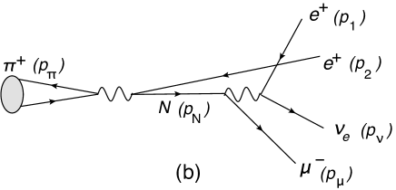
Figure 8: The lepton number conserving (LNC) process $\pi^{+}\to e^{+}N\to e^{+}\mu^{-}e^{+}\nu_{e}$ which can be mediated by a Dirac or a Majorana on-shell neutrino $N$: (a) the direct ($D$) channel; (b) the crossed ($C$) channel.

The considered processes are presented in Figures 8 and 9. As in the previous Section, we consider a scenario with at least one heavy sterile neutrino $N$, which has suppressed heavy-light mixing coefficients $B_{\ell N}$ with the first three neutrino flavors $\nu_{\ell}$ ($\ell=e,\mu,\tau$), cf. Equation (1). The mentioned decay rates may be nonnegligible only if the intermediate neutrino $N$ is on-shell, i.e.,

$$(M_{\mu}+M_{e})<M_{N}<(M_{\pi}-M_{e})\$$ (35)

and the process is of the $s$-type, Figures 8 and 9. Specifically, this means $106.2\ {\rm MeV}<M_{N}<139\ {\rm MeV}$.

Figure 9: The lepton number violating (LNV) process $\pi^{+}\to e^{+}N\to e^{+}e^{+}\mu^{-}{\overline{\nu}}_{\mu}$ which can be mediated by a neutrino $N$ only if $N$ is a Majorana particle: (a) the direct (D) channel; (b) the crossed (C) channel.

III.1 Branching Ratios for $\pi^{\pm}\to e^{\pm}e^{\pm}\mu^{\mp}\nu$

The decay widths $\Gamma^{{\rm(X)}}(\pi^{\pm}\to e^{\pm}e^{\pm}\mu^{\mp}\nu)$ (X=LNC, LNV) can be written in terms of the corresponding reduced decay amplitudes ${\cal T}_{\pi,\pm}^{{\rm(X)}}$

$$\Gamma^{\rm(X)}(\pi^{\pm}\to e^{\pm}e^{\pm}\mu^{\mp}\nu)=\frac{1}{2!}\frac{1}{2M_{\pi}}\frac{1}{(2\pi)^{8}}\int d_{4}\;|{\cal T}_{\pi,\pm}^{\rm(X)}|^{2}\$$ (36)

Here, $1/2!$ represents the symmetry factor from two final state electrons, and $d_{4}$ is the integration element of the phase space of the four final particles

$$d_{4}=\left(\prod_{j=1}^{2}\frac{d^{3}{\vec{p}}_{j}}{2E_{e}({\vec{p}}_{j})}\right)\frac{d^{3}{\vec{p}}_{\mu}}{2E_{\mu}({\vec{p}}_{\mu})}\frac{d^{3}{\vec{p}}_{\nu}}{2|{\vec{p}}_{\nu}|}\delta^{(4)}\left(p_{\pi}-p_{1}-p_{2}-p_{\mu}-p_{\nu}\right)\$$ (37)

Here, $p_{1}$ and $p_{2}$ are the momenta of $e$; in the direct channel, the $e$ momentum at the first (left-hand) vertex is $p_{1}$, and in the crossed channel it is $p_{2}$, cf. Figures 8 and 9. When we use the expressions for the amplitudes ${\cal T}_{\pi,\pm}^{{\rm(X)}}$ of Appendix 4, for the specific considered case $N_{1}=N$ (and no $N_{2}$), the decay width (36) can be written as

$$\Gamma^{\rm(X)}(\pi^{\pm}\to e^{\pm}e^{\pm}\mu^{\mp}\nu) = |k^{\rm(X)}|^{2}{\big{[}}{\widetilde{\Gamma}}_{\pi}^{\rm(X)}(DD^{*})+{\widetilde{\Gamma}}_{\pi}^{\rm(X)}(CC^{*})+{\widetilde{\Gamma}}_{{\pi},\pm}^{\rm(X)}(DC^{*})+{\widetilde{\Gamma}}_{{\pi},\pm}^{\rm(X)}(CD^{*}{\big{]}}\$$ (38)

where X = LNC, LNV; $k_{\pm}^{\rm(X)}$ are the corresponding mixing factors

$$k^{{\rm(LNV)}}=B_{eN}^{2}\ ,\qquad k^{{\rm(LNC)}}=B_{eN}B^{*}_{\mu N}\$$ (39)

and ${\widetilde{\Gamma}}_{\pi}^{{\rm(X)}}(YZ^{*})$ are the normalized (i.e., without explicit mixing dependence) decay widths

$${\widetilde{\Gamma}}_{{\pi},\pm}^{{\rm(X)}}(YZ^{*})=K_{\pi}^{2}\;\frac{1}{2!}\frac{1}{2M_{\pi}}\frac{1}{(2\pi)^{8}}\int d_{4}\;P^{{\rm(X)}}(Y)P^{{\rm(X)}}(Z)^{*}\;T_{{\pi},\pm}^{{\rm(X)}}(YZ^{*})\$$ (40)

The expressions for $T_{{\pi},\pm}^{{\rm(X)}}(YZ^{*})$ are given in Appendix 4, for the direct ($YZ^{*}=DD^{*}$), crossed ($YZ^{*}=CC^{*}$) and direct-crossed interference contributions ($YZ^{*}=DC^{*}$, $CD^{*}$). We have $T_{{\pi},+}^{{\rm(X)}}(DD^{*})=T_{{\pi},-}^{{\rm(X)}}(DD^{*})$ and $T_{{\pi},+}^{{\rm(X)}}(CC^{*})=T_{{\pi},-}^{{\rm(X)}}(CC^{*})$, hence the terms ${\widetilde{\Gamma}}_{\pi}^{{\rm(X)}}(DD^{*})$ and ${\widetilde{\Gamma}}_{\pi}^{{\rm(X)}}(CC^{*})$ in Equation (38) have no subscripts $\pm$. Further, in Equation (40), $P^{{\rm(X)}}(Y)$ represent the $N$ propagator functions of the direct and crossed channels ($Y=D,C$)

$$P^{\rm({\rm LNC})}(D) = \frac{1}{\left[(p_{\pi}-p_{1})^{2}-M_{N}^{2}+i\Gamma_{N}M_{N}\right]},\qquad P^{\rm({\rm LNV})}(D)=M_{N}P^{\rm({\rm LNC})}(D)$$ (41a)

$$P^{\rm({\rm LNC})}(C) = \frac{1}{\left[(p_{\pi}-p_{2})^{2}-M_{N}^{2}+i\Gamma_{N}M_{N}\right]},\qquad P^{\rm({\rm LNV})}(C)=M_{N}P^{\rm({\rm LNC})}(C)$$ (41b)

where $\Gamma_{N}\equiv\Gamma(N\to{\rm all})$, and $K_{\pi}^{2}$ is the following constant:

$$K_{\pi}^{2}=G_{F}^{4}f_{\pi}^{2}|V_{ud}|^{2}\approx 2.983\times 10^{-22}\ {\rm GeV}^{-6}\$$ (42)

It turns out that in the case when the intermediate $N$ neutrino is on-shell, i.e., when its mass is in the interval of Equation (35), the squares of the propagators (41) reduce to simple delta functions due to the inequality $\Gamma_{N}\ll M_{N}$

$$|P^{\rm(LNC)}(X)|^{2} = \left|\frac{1}{(p_{\pi}-p_{k})^{2}-M^{2}_{N}+i\Gamma_{N}M_{N}}\right|^{2}$$ (43)

$$= \frac{\pi}{M_{N}\Gamma_{N}}\delta((p_{\pi}-p_{k})^{2}-M^{2}_{N})\quad(\Gamma_{N}\ll M_{N})\$$

where $p_{k}=p_{1},p_{2}$ for $X=D,C$. In this on-shell case, the $DD^{*}$ and $CC^{*}$ contributions in Equation (38) are large and equal, and the interference contributions $DC^{*}$ and $CD^{*}$ are negligible in comparison; we refer to CKZ for details on this point. Hence the decay width (38) can be written in the on-shell case as

$$\Gamma^{{\rm(X)}}(\pi^{\pm}\to e^{\pm}e^{\pm}\mu^{\mp}\nu) = 2|k^{\rm(X)}|^{2}{\widetilde{\Gamma}}(\pi^{\pm}\to e^{\pm}e^{\pm}\mu^{\mp}\nu)\$$ (44)

Here, the normalized decay width ${\widetilde{\Gamma}}_{\pi}^{{\rm(X)}}(DD^{*})={\widetilde{\Gamma}}_{\pi}^{{\rm(X)}}(CC^{*})\equiv{\widetilde{\Gamma}}(\pi^{\pm}\to e^{\pm}e^{\pm}\mu^{\mp}\nu)$ turns out to be the same for X = LNC and X = LNV,

$${\widetilde{\Gamma}}(\pi^{\pm}\to e^{\pm}e^{\pm}\mu^{\mp}\nu)\equiv{\widetilde{\Gamma}}_{\pi}^{{\rm(X)}}(DD^{*})\equiv{\widetilde{\Gamma}}_{\pi}(CC^{*})$$ (45)

$$=\frac{K_{\pi}^{2}}{192(2\pi)^{4}}\frac{M_{N}^{11}}{M_{\pi}^{3}\Gamma_{N}}\lambda^{1/2}(x_{\pi},1,x_{e})\left[x_{\pi}-1+x_{e}(x_{\pi}+2-x_{e})\right]{\cal F}(x_{\mu},x_{e})$$

where the following notations are used:

$$\lambda(y_{1},y_{2},y_{3}) = y_{1}^{2}+y_{2}^{2}+y_{3}^{2}-2y_{1}y_{2}-2y_{2}y_{3}-2y_{3}y_{1}\$$ (46a)

$$x_{\pi} = \frac{M_{\pi}^{2}}{M_{N}^{2}}\ ,\quad x_{e}=\frac{M_{e}^{2}}{M_{N}^{2}}\ ,\quad x_{\mu}=\frac{M_{\mu}^{2}}{M_{N}^{2}}\$$ (46b)

and the function ${\cal F}(x_{\mu},x_{e})$ is given in Appendix 5. In the approximation $M_{e}=0$, the above result becomes simpler

$$\lim_{M_{e}\to 0}{\widetilde{\Gamma}}(\pi^{\pm}\to e^{\pm}e^{\pm}\mu^{\mp}\nu)=\frac{K_{\pi}^{2}}{192(2\pi)^{4}}\frac{M_{N}^{11}}{\Gamma_{N}M_{\pi}^{3}}(x_{\pi}-1)^{2}f(x_{\mu})\$$ (47)

where the function $f(x_{\mu})={\cal F}(x_{\mu},0)$ is

$$f(x_{\mu})=1-8x_{\mu}+8x_{\mu}^{3}-x_{\mu}^{4}-12x_{\mu}^{2}\ln x_{\mu}\$$ (48)

It can be checked that the decay rate (44), with $N$ on shell, coincides with the factorized expression

$$\Gamma(\pi^{+}\to e^{+}e^{+}\mu^{-}\nu)=\Gamma(\pi^{+}\to e^{+}N){\rm Br}(N\to e^{+}\mu^{-}\nu)\$$ (49)

In Appendix 5 we also provide the differential decay rates $d\Gamma^{{\rm(X)}}(\pi^{\pm}\to e^{\pm}e^{\pm}\mu^{\mp}\nu)/dE_{\mu}$ with respect to the final muon energy in the rest frame of $N$ neutrino. They turn out to have quite different forms for X = LNC and X = LNV cases (we will return to this later in this Section).

In order to obtain the branching fractions of the considered processes, we need to divide the decay width by the total decay width of the charged pion, $\Gamma(\pi^{\pm}\to{\rm all})$

$$\Gamma(\pi^{+}\to{\rm all}) = 2.529\times 10^{-17}\ {\rm GeV}$$ (50a)

$$\approx \frac{1}{8\pi}G^{2}_{F}f^{2}_{\pi}M^{2}_{\mu}M_{\pi}|V_{ud}|^{2}\left(1-\frac{M^{2}_{\mu}}{M^{2}_{\pi}}\right)^{2}\left(1+\delta g_{\pi}\right)\$$ (50b)

where the expression (50b) represents the by far most dominant decay mode $\pi^{\pm}\to\mu^{\pm}\nu_{\mu}$, and

$$\delta g_{\pi}=\frac{M_{e}^{2}}{M_{\mu}^{2}}\frac{(1-M_{e}^{2}/M_{\pi}^{2})^{2}}{(1-M_{\mu}^{2}/M_{\pi}^{2})^{2}}\$$ (51)

represents a (very small) relative correction coming from the $\pi^{\pm}\to e^{\pm}\nu_{e}$ decay ($\delta g_{\pi}\approx 1.3\times 10^{-4}$).

As we can see in Equations (44) and (45), the decay width $\Gamma(\pi^{\pm}\to e^{\pm}e^{\pm}\mu^{\mp}\nu)$ and its normalized counterpart ${\widetilde{\Gamma}}(\pi^{\pm}\to e^{\pm}e^{\pm}\mu^{\mp}\nu)$ are inversely proportional to the (very small) decay width $\Gamma(N\to{\rm all})\equiv\Gamma_{N}$, which in turn is proportional to the mixings ${\widetilde{\cal K}}\sim|B_{\ell N}|^{2}$ ($\ell=e,\mu,\tau$), cf. Equations (16)–(18) and Figure 2. As in Section II.1, this effect represents the $N$-on-shell effect Equation (43) and it makes the considered width $\Gamma(\pi^{\pm}\to e^{\pm}e^{\pm}\mu^{\mp}\nu)$ by many orders of magnitude larger than it would be in the case of off-shell $N$. In the (narrow) mass interval (35) for on-shell $N$ in the considered pion decays, the factor ${\widetilde{\cal K}}$ in the width $\Gamma_{N}$ Equation (16) has the following approximate form (cf. Appendix 3 and Figure 2):

$${\widetilde{\cal K}}(\pi^{\pm}\to e^{\pm}e^{\pm}\mu^{\mp}\nu)\approx 1.6|B_{eN}|^{2}+1.1(|B_{\mu N}|^{2}+|B_{\tau N}|^{2})$$ (52)

This expression, within the precision given here, is valid equally for the Majorana and for the Dirac $N$ and agrees with that given in Ref. CKZ for the Majorana case. However, the affirmation in Ref. CKZ that ${\widetilde{\cal K}}$ for Dirac $N$ is smaller by a factor of two is not correct.

In certain analogy with Section II.1, we can define here the canonical branching ratio ${\overline{\rm Br}}_{\pi}$ as the part of the branching ratio ${\rm Br}^{\rm(X)}_{\pi}\equiv\Gamma(\pi^{\pm}\to e^{\pm}e^{\pm}\mu^{\mp}\nu)/\Gamma(\pi\to{\rm all})$ which contains no explicit or implicit heavy-light mixing dependence (and is independent of X = LNC or LNV)

$${\overline{\rm Br}}_{\pi} \equiv 2\frac{{{\widetilde{\cal K}}}}{\Gamma_{\pi}}{\widetilde{\Gamma}}(\pi^{\pm}\to e^{\pm}e^{\pm}\mu^{\mp}\nu)=\frac{{\widetilde{\cal K}}}{|k^{\rm(X)}|^{2}}{\rm Br}^{\rm(X)}(\pi^{\pm}\to e^{\pm}e^{\pm}\mu^{\mp}\nu)$$ (53a)

$$= \frac{1}{16\pi}\frac{K_{\pi}^{2}M_{\pi}^{3}}{G_{F}^{2}\Gamma(\pi^{+}\to{\rm all})}\frac{1}{x_{\pi}^{3}}\lambda^{1/2}(x_{\pi},1,x_{e})\left[x_{\pi}-1+x_{e}(x_{\pi}+2-x_{e})\right]{\cal F}(x_{\mu},x_{e})$$ (53b)

$$= \frac{1}{2}\frac{1}{x_{\mu}(x_{\pi}-x_{\mu})^{2}(1+\delta g_{\pi})}\lambda^{1/2}(x_{\pi},1,x_{e})\left[x_{\pi}-1+x_{e}(x_{\pi}+2-x_{e})\right]{\cal F}(x_{\mu},x_{e})\$$ (53c)

where the notations (46) are used, and in Equation (53c) we used the expression (125) in Appendix 5. We note that ${\widetilde{\cal K}}\sim|B_{\ell N}|^{2}$ and $|k^{\rm(X)}|^{2}\sim|B_{\ell N}|^{4}$, and ${\rm Br}^{\rm(X)}_{\pi}\propto|k^{\rm(X)}|^{2}/{\widetilde{\cal K}}\sim|B_{\ell N}|^{2}$, where $B_{\ell N}$ stands for a generic heavy-light mixing coefficient ($|B_{\ell N}|\sim|B_{eN}|\sim|B_{\mu N}|$). Naively, we should have very strong suppression ${\rm Br}^{\rm(X)}_{\pi}\propto|k^{\rm(X)}|^{2}\propto|B_{\ell N}|^{4}$; however, the on-shellness (43) brings in factor $1/\Gamma_{N}\propto 1/{\widetilde{\cal K}}\sim 1/|B_{\ell N}|^{2}$, reducing the suppression to ${\rm Br}^{\rm(X)}_{\pi}\propto|B_{\ell N}|^{2}$. In Figure 10 we present the canonical branching fraction ${\overline{\rm Br}}_{\pi}$ as a function of $M_{N}$ in the entire interval of on-shellness (35). In Figure 11 this canonical branching fraction is presented at the lower edge of the on-shellness interval, where the effects of $M_{e}\not=0$ turn out to be appreciable. We can see that the branching ratio is the largest when $M_{N}\approx 0.130$ GeV.

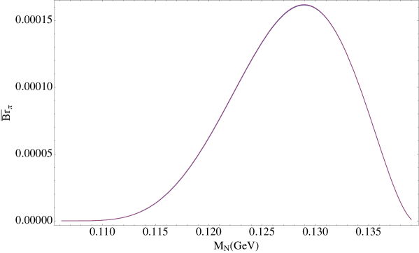
Figure 10: The canonical branching ratio ${\overline{\rm Br}}_{\pi}$, Equation (53), as a function of the mass $M_{N}$. The full formula was used (with $M_{e}=0.511\times 10^{-3}$ GeV). The formula for $M_{e}=0$ case gives a line which is in this Figure indistinguishable from the depicted line.

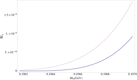
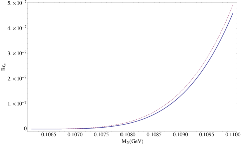
Figure 11: The canonical branching ratio ${\overline{\rm Br}}_{\pi}$ near the lower end point $M_{\mu}+M_{e}$ (=$0.1062$ GeV): (a) in the interval below $0.107$ GeV; (b) in the interval below $0.110$ GeV. The dashed line is for $M_{e}=0$, the full line includes the effects of $M_{e}=0.511\times 10^{-3}$ GeV.

The differential branching ratios $d{\rm Br}^{\rm(X)}/dE_{\mu}$, where $E_{\mu}$ is the final muon energy in the $N$-rest frame, are obtained directly from the differential branching ratios $d{\widetilde{\Gamma}}_{\pi}^{\rm(X)}/dE_{\mu}$, and the latter quantity for X = LNV is given explicitly in Appendix 5. The canonical differential branching ratios, free of any mixing dependence, can be defined in analogy with the definition of the canonical total branching ratio (53a), and, in contrast to canonical branching ratios (53) they do depend on whether X = LNC or X = LNV

$$\frac{d{\overline{\rm Br}_{\pi}^{\rm(X)}}}{dE_{\mu}} \equiv 2\frac{{{\widetilde{\cal K}}}}{\Gamma_{\pi}}\frac{d{\widetilde{\Gamma}}(\pi^{\pm}\to e^{\pm}e^{\pm}\mu^{\mp}\nu)}{dE_{\mu}}=\frac{{\widetilde{\cal K}}}{|k^{\rm(X)}|^{2}}\frac{d{\rm Br}^{\rm(X)}(\pi^{\pm}\to e^{\pm}e^{\pm}\mu^{\mp}\nu)}{dE_{\mu}}$$ (54)

Explicit expressions for these quantities, when X = LNV and X = LNC, are given in Appendix 5 in Equations (126) and (128), and in the limit $M_{e}=0$ in Equation (129).

The differential (and full) branching ratios for the process $\pi^{\pm}\to e^{\pm}e^{\pm}\mu^{\mp}\nu$ differ in the cases when the on-shell $N$ is Majorana or Dirac. When $N$ is Dirac, only the X = LNC process contributes. When $N$ is Majorana, both LNC and LNV processes contribute. We can write the differential and full branching ratios in these cases in terms of their canonical counterparts, by defining first the combined canonical differential branching ratios

$$\frac{d{\overline{\rm Br}}_{\pi}(\alpha)}{dE_{\mu}}\equiv\alpha\frac{d{\overline{\rm Br}}_{\pi}^{\rm(LNV)}}{dE_{\mu}}+(1-\alpha)\frac{d{\overline{\rm Br}}_{\pi}^{\rm(LNC)}}{dE_{\mu}}\$$ (55)

where $0\leq\alpha\leq 1$. Then it is straightforward to check that in the cases of Dirac and Majorana $N$ neutrino, the branching ratios can be expressed in terms of the above quantites (55)

$$\frac{d{\rm Br}^{\rm(Dir.)}(\pi^{\pm}\to e^{\pm}e^{\pm}\mu^{\mp}\nu)}{dE_{\mu}} = \frac{|k^{\rm(LNC)}|^{2}}{{\widetilde{\cal K}}^{\rm(Dir.)}}\frac{d{\overline{\rm Br}}_{\pi}(\alpha=0)}{dE_{\mu}}\$$ (56a)

$$\frac{d{\rm Br}^{\rm(Maj.)}(\pi^{\pm}\to e^{\pm}e^{\pm}\mu^{\mp}\nu)}{dE_{\mu}} = \frac{(|k^{\rm(LNV)}|^{2}+|k^{\rm(LNC)}|^{2})}{{\widetilde{\cal K}}^{\rm(Maj.)}}\frac{d{\overline{\rm Br}}_{\pi}(\alpha_{M})}{dE_{\mu}}\$$ (56b)

where we recall the definition (39) of the coefficients $k^{\rm(X)}$, and the “Majorana LNV admixture” parameter $\alpha_{M}$ appearing in Equation (56b) is defined as

$$\alpha_{M}=\frac{|k^{\rm(LNV)}|^{2}}{(|k^{\rm(LNV)}|^{2}+|k^{\rm(LNC)}|^{2})}=\frac{|B_{eN}|^{2}}{(|B_{eN}|^{2}+|B_{\mu N}|^{2})}\$$ (57)

Integration of the relations (56) over $E_{\mu}$ leads to the full branching ratios

$${\rm Br}^{\rm(Dir.)}(\pi^{\pm}\to e^{\pm}e^{\pm}\mu^{\mp}\nu) = \frac{|k^{\rm(LNC)}|^{2}}{{\widetilde{\cal K}}^{\rm(Dir.)}}{\overline{\rm Br}}_{\pi}=\frac{|B_{eN}|^{2}|B_{\mu N}|^{2}}{\sum_{\ell=e,\mu,\tau}{\cal N}^{\rm(Dir.)}_{\ell N}|B_{\ell N}|^{2}}{\overline{\rm Br}}_{\pi},$$ (58a)

$${\rm Br}^{\rm(Maj.)}(\pi^{\pm}\to e^{\pm}e^{\pm}\mu^{\mp}\nu) = \frac{(|k^{\rm(LNV)}|^{2}\!+\!|k^{\rm(LNC)}|^{2})}{{\widetilde{\cal K}}^{\rm(Maj.)}}{\overline{\rm Br}}_{\pi}=\frac{|B_{eN}|^{2}(|B_{eN}|^{2}\!+\!|B_{\mu N}|^{2})}{\sum_{\ell=e,\mu,\tau}{\cal N}^{\rm(Maj.)}_{\ell N}|B_{\ell N}|^{2}}{\overline{\rm Br}}_{\pi}$$ (58b)

where we used the fact that the $E_{\mu}$-integrated expression ${\overline{\rm Br}}_{\pi}(\alpha)$ is independent of $\alpha$, cf. Equations (53). In Figures 12 we present these canonical differential branching ratios as a function of the muon energy $E_{\mu}$ in the rest frame of $N$, for four different values of mass $M_{N}$ in the on-shell interval (35), and for five different values of the admixture parameter ($\alpha_{M}=1,$ 0.8, 0.5, 0.2 and 0), The value $\alpha_{M}=0$ corresponds to the case of Dirac $N$. From the curves of Figure 12 we can conclude: if $N$ is Majorana neutrino with a significant value of the admixture parameter $\alpha_{M}$ and with mass in the interval (35), then the measurement of such differential branching ratios may be able to confirm the Majorana nature of $N$.

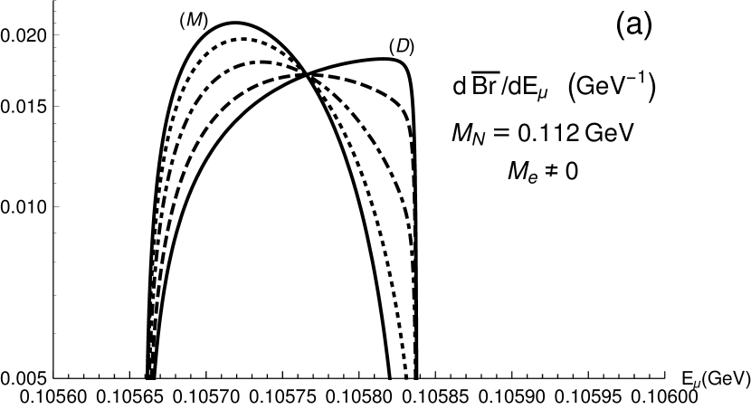
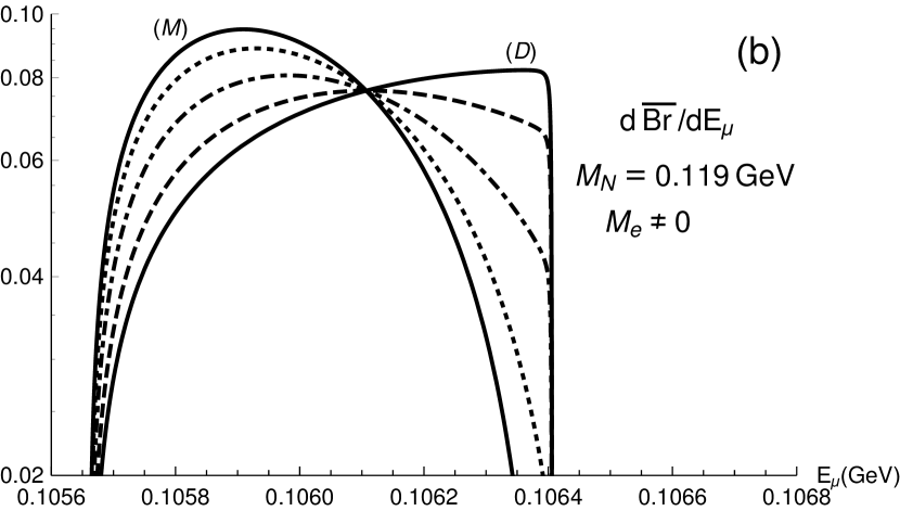
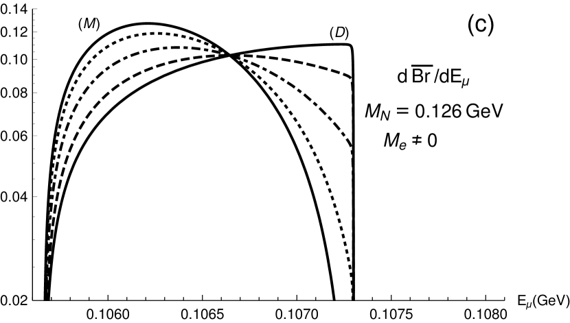
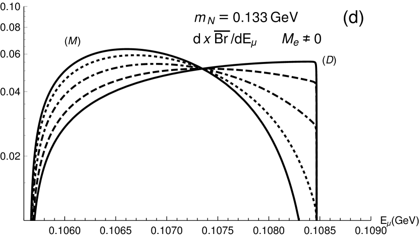
Figure 12: The canonical differential branching ratio $d{\overline{\rm Br}}_{\pi}(\alpha_{M})/dE_{\mu}$ as a function of the muon energy in the neutrino $N$ rest frame, $E_{\mu}$, as defined via Equations (55), for the decays $\pi^{\pm}\to e^{\pm}e^{\pm}\mu^{\mp}{\nu}$ mediated by a Majorana neutrino $N$, for various neutrino masses: (a) $M_{N}=0.112$ GeV; (b) $M_{N}=0.119$ GeV; (c) $M_{N}=0.126$ GeV; (d) $M_{N}=0.133$ GeV. In each graph there are five curves, corresponding to different values of the admixture parameter $\alpha_{M}$ [Equation (57)]: $\alpha_{M}=1.0$ is the solid (M) curve; $0.8$ (dotted); $0.5$ (dot-dashed); $0.2$ (dashed). The case mediated by a Dirac neutrino ($\alpha_{M}=0$) is also presented as the solid line labelled (D). In comparison with Fig. 5 of Ref. CDK (where $M_{e}=0$ was taken and linear $y$-scale was used), the true value of $M_{e}=0.511$ MeV is taken here and logarithmic $y$-scale is used.

If the differential branching ratios are studied with respect to the muon energy $E^{{}^{\prime}}_{\mu}$ in the pion rest frame, the distinction between the Dirac and Majorana case is more difficult, cf. Ref. CDK .

III.2 Effect of the Long Neutrino Lifetime on the Observability of $\pi^{\pm}\to e^{\pm}e^{\pm}\mu^{\mp}\nu$

The branching ratios presented in this Section so far, Equations (58) in conjunction with Equations (53), should be multiplied by the probability $P_{N}$ for the on-shell neutrino $N$ to decay within the detector (of length $L$), as explained in Section II.2, Equations (22)–(26) and Figure 3. As a consequence, the effective (true, measurable) branching ratios are not ${\rm Br}$ ($\sim|B_{\ell N}|^{2}$) of Equations (58), but ${\rm Br}_{\rm eff}=P_{N}{\rm Br}$

$${\rm Br}_{\rm eff}^{\rm(Dir.)}(\pi^{\pm}\to e^{\pm}e^{\pm}\mu^{\mp}\nu) = P_{N}^{\rm(Dir.)}{\rm Br}^{\rm(Dir.)}(\pi^{\pm}\to e^{\pm}e^{\pm}\mu^{\mp}\nu)$$ (59a)

$$= \left[{\overline{P}}_{N}\left(\frac{L}{1{\rm m}}\right){\widetilde{\cal K}}^{\rm(Dir.)}\right]\left[\frac{|B_{eN}|^{2}|B_{\mu N}|^{2}}{{\widetilde{\cal K}}^{\rm(Dir.)}}{\overline{\rm Br}}_{\pi}\right]$$

$$= |B_{eN}|^{2}|B_{\mu N}|^{2}\left(\frac{L}{1{\rm m}}\right){\overline{P}}_{N}{\overline{\rm Br}}_{\pi}=|B_{eN}|^{2}|B_{\mu N}|^{2}\left(\frac{L}{1{\rm m}}\right){\overline{\rm Br}}_{\pi,{\rm eff}}$$ (59b)

$${\rm Br}_{\rm eff}^{\rm(Maj.)}(\pi^{\pm}\to e^{\pm}e^{\pm}\mu^{\mp}\nu)=P_{N}^{\rm(Maj.)}{\rm Br}^{\rm(Maj.)}(\pi^{\pm}\to e^{\pm}e^{\pm}\mu^{\mp}\nu)$$ (60a)

$$= \left[{\overline{P}}_{N}\left(\frac{L}{1{\rm m}}\right){\widetilde{\cal K}}^{\rm(Maj.)}\right]\left[\frac{|B_{eN}|^{2}(|B_{eN}|^{2}+|B_{\mu N}|^{2})}{{\widetilde{\cal K}}^{\rm(Maj.)}}{\overline{\rm Br}}_{\pi}\right]$$

$$= |B_{eN}|^{2}(|B_{eN}|^{2}+|B_{\mu N}|^{2})\left(\frac{L}{1{\rm m}}\right){\overline{P}}_{N}{\overline{\rm Br}}_{\pi}=|B_{eN}|^{2}(|B_{eN}|^{2}+|B_{\mu N}|^{2})\left(\frac{L}{1{\rm m}}\right){\overline{\rm Br}}_{\pi,{\rm eff}}$$ (60b)

In Equations (59a) and (60a) we used the expressions (58) for ${\rm Br}$ and Equation (26) for $P_{N}$. In Equations (59b) and (60b) we introduced canonical (i.e., without any mixing dependence) effective branching ratio ${\overline{\rm Br}}_{\pi,{\rm eff}}$

$${\overline{\rm Br}}_{\pi,{\rm eff}}\equiv{\overline{P}}_{N}{\overline{\rm Br}}_{\pi}\$$ (61)

with ${\overline{\rm Br}}_{\pi}$ given in Equations (53), and the canonical nonsurvival probability ${\overline{P}}_{N}$ presented in Figure 3 in Section II.2 for a wide range of $N$ neutrino masses. In Figure 13 we present ${\overline{P}}_{N}$ in the here relevant narrower mass interval (35).

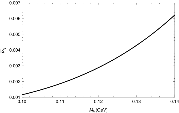
Figure 13: The canonical probability ${\overline{P}}_{N}\equiv(1{\rm m})/{\overline{L}}_{N}$, Equation (26), as a function of the neutrino mass $M_{N}$ in the approximate interval where it is on shell (35) for decays $\pi^{\pm}\to e^{\pm}e^{\pm}\mu^{\mp}\nu$. The Lorentz lab time dilation factor is chosen to be $\gamma_{N}$ [$\equiv(1-\beta_{N}^{2})^{-1/2}$] $=2$.

As in the case of semileptonic LNV decays of Section II.2, we notice that also here in the effective branching ratios, Equations (59) and (60), the complicated dependence on the mixing parameters entailed by the factors ${\widetilde{\cal K}}=\sum_{\ell}{\cal N}_{\ell N}|B_{\ell N}|^{2}$ of $\Gamma_{N}$ [cf. Equation (18)], cancels out, and there remains only simple dependence on the mixing parameters, in the form $|B_{eN}|^{2}|B_{\mu N}|^{2}$ or $|B_{eN}|^{2}(|B_{eN}|^{2}+|B_{\mu N}|^{2})$. Further, in comparison with the branching ratios ${\rm Br}$ of Equations (58), which are $\sim|B_{\ell N}|^{2}$, the effective (true) branching ratios ${\rm Br}_{\rm eff}$ of Equations (59) and (60) are unfortunately significantly more suppressed by the mixing parameters, namely ${\rm Br}_{\rm eff}\sim|B_{\ell N}|^{4}$.

The presently known experimental bounds on the mixing parameters $|B_{\ell N}|^{2}$ ($\ell=e,\mu,\tau$) in the here relevant narrow mass range (35), are: $|B_{eN}|^{2}\lesssim 10^{-8}$ PIENU:2011aa ; $|B_{\mu N}|^{2}\lesssim 10^{-6}$ BmuN ; BmuN2 ; BmuN3 ; $|B_{\tau N}|^{2}\lesssim 10^{-4}$ BtauN ; cf. also Refs. Atre ; Ruchayskiy:2011aa ; 1502.00477 ; Devlimits .

The future pion factories, such as the Project X at Fermilab, will be designed to produce charged pions with lab energies $E_{\pi}$ of a few GeV and luminosities $\sim 10^{22}\ {\rm cm}^{-2}{\rm s}^{-1}$ ProjX ; Geer , and $\sim 10^{29}$ charged pions could be expected per year.

The canonical effective branching ratio (61) can be estimated as

$${\overline{\rm Br}}_{\pi,{\rm eff}}\lesssim 10^{-6}$$ (62)

as can be inferred from Equation (61) and Figures 13 and 10. Equations (59) and (60) then imply that the effective (true) branching ratios for the considered reactions are (we assume $L=1{\rm\,m}$ for the detector length)

$${\rm Br}_{\rm eff}^{\rm(Dir.)} \lesssim |B_{eN}|^{2}|B_{\mu N}|^{2}10^{-6},$$ (63a)

$${\rm Br}_{\rm eff}^{\rm(Maj.)} \lesssim |B_{eN}|^{2}(|B_{eN}|^{2}+|B_{\mu N}|^{2})10^{-6}$$ (63b)

If the larger among the mixing elements ($|B_{\ell N}|^{2}$, $\ell=e,\mu$) is $|B_{\mu N}|^{2}$ ($\lesssim 10^{-6}$), the LNC processes dominate, and the effective branching ratios (63) have the common upper bounds

$${\rm Br}_{\rm eff}^{\rm(Dir.,Maj.)}\lesssim|B_{eN}|^{2}|B_{\mu N}|^{2}10^{-6}\lesssim|B_{eN}|^{2}10^{-12}$$ (64)

If in this case $|B_{eN}|^{2}$ is close to its present upper bound, $|B_{eN}|^{2}\sim 10^{-8}$, we obtain ${\rm Br}_{\rm eff}^{\rm(Dir.,Maj.)}\lesssim 10^{-20}$. This implies that up to $10^{9}$ events $\pi^{\pm}\to e^{\pm}e^{\pm}\mu^{\mp}\nu$ could be detected per year in such a scenario.

On the other hand, if the larger among the mixing elements ($B_{\ell N}|^{2}$, $\ell=e,\mu$) is $|B_{eN}|^{2}$ ($\lesssim 10^{-8}$), the LNV processes dominate, and the effective branching ratios (63) have the following upper bounds:

$${\rm Br}_{\rm eff}^{\rm(Dir.)} \lesssim |B_{\mu N}|^{2}10^{-14}$$ (65a)

$${\rm Br}_{\rm eff}^{\rm(Maj.)} \lesssim 10^{-22}$$ (65b)

In such a case we have $|B_{\mu N}|^{2}<|B_{eN}|^{2}\lesssim 10^{-8}$, and up to $10^{7}$ events could be detected per year.

The present upper bounds on $|B_{\ell N}|^{2}$ suggest that the first scenario, Equation (64), is more likely.

The measurement of the effective branching ratios alone cannot distinguish between the Dirac and the Majorana character of intermediate neutrino $N$. However, as argued in Section III.1 and presented in Figure 12, the measurement of the differential branching ratios for the considered processes is a promising way to discern the character of the neutrinos. However, the differential branching ratios (56) must be multiplied by the nonsurvival probability $P_{N}$, in order to obtain the effective (true, measurable) differential branching ratios $d{\rm Br}_{\rm eff}/dE_{\mu}$. In analogy with Equations (59) and (60) we obtain, using Equation (56)

$$\frac{d{\rm Br}_{\rm eff}^{\rm(Dir.)}(\pi^{\pm}\to e^{\pm}e^{\pm}\mu^{\mp}\nu)}{dE_{\mu}} = P_{N}\frac{d{\rm Br}^{\rm(Dir.)}(\pi^{\pm}\to e^{\pm}e^{\pm}\mu^{\mp}\nu)}{dE_{\mu}}$$ (66a)

$$= |B_{eN}|^{2}|B_{\mu N}|^{2}\left(\frac{L}{1{\rm m}}\right)\frac{d{\overline{\rm Br}}_{\pi,{\rm eff}}(\alpha=0)}{dE_{\mu}}$$

$$\frac{d{\rm Br}_{\rm eff}^{\rm(Maj.)}(\pi^{\pm}\to e^{\pm}e^{\pm}\mu^{\mp}\nu)}{dE_{\mu}} = P_{N}\frac{d{\rm Br}^{\rm(Maj.)}(\pi^{\pm}\to e^{\pm}e^{\pm}\mu^{\mp}\nu)}{dE_{\mu}}$$ (66b)

$$= |B_{eN}|^{2}(|B_{eN}|^{2}+|B_{\mu N}|^{2})\left(\frac{L}{1{\rm m}}\right)\frac{d{\overline{\rm Br}}_{\pi,{\rm eff}}(\alpha_{M})}{dE_{\mu}}$$

where the canonical differential effective branching ratios were introduced, in analogy with Equation (55)

$$\frac{d{\overline{\rm Br}}_{\pi,{\rm eff}}(\alpha)}{dE_{\mu}}\equiv{\overline{P}}_{N}\frac{d{\overline{\rm Br}}_{\pi}(\alpha)}{dE_{\mu}}\$$ (67)

with $d{\overline{\rm Br}}_{\pi}(\alpha)/dE_{\mu}$ given in Equation (55). The parameter $\alpha_{M}$ appearing in Equation (66b) was defined in Equation (57). In analogy with Figure 12, and using the values of ${\overline{P}}_{N}$ from Figure 13, we deduce that the values of the $y$-axes of Figure 12a–d, must be multiplied by ${\overline{P}}_{N}\approx 2.0\times 10^{-3}$, $2.8\times 10^{-3}$, $3.7\times 10^{-3}$, and $4.8\times 10^{-3}$, respectively (assuming $L=1$ m and $\gamma_{N}=2$), in order to obtain the representation for the curves of the canonical differential effective ratios $d{\overline{\rm Br}}_{\pi,{\rm eff}}(\alpha)/dE_{\mu}$.

IV CP Violation in Charged Meson Decays Mediated by Massive Sterile Neutrinos

CP violation in the lepton sector could be measured by neutrino oscillations oscCP . Here we consider the possibilities of measuring CP violation in meson decays mediated by sterile neutrinos $N$, such as the semileptonic LNV decays of charged heavy pseudoscalar mesons considered in Section II, or the leptonic (LNV and LNC) decays of charged pions considered in Section III.

It turns out that CP violation in all such decays is possible in scenarios with at least two massive sterile neutrinos $N_{j}$ ($j=1,2$). CP violation in the neutrino sector is expected whether neutrinos are Dirac or Majorana particles. However, in the Pontecorvo–Maki–Nakagawa–Sakata (PMNS) mixing matrix Pontecorvo ; Pontecorvo2 ; MNS , the number of possible CP-violating phases is larger when the neutrinos are Majorana particles. If $n=3+{\cal N}$ is the total number of neutrinos (${\cal N}$ is the number of sterile neutrinos), the number of CP-violating phases is $n(n-1)/2$ if neutrinos are Majorana, and $(n-1)(n-2)/2$ if neutrinos are Dirac, cf. Ref. Bilenky .

CP violation in the decays $\pi^{\pm}\to e^{\pm}N_{j}\to e^{\pm}e^{\pm}\mu^{\mp}\nu$ was investigated in Ref. CKZ , and in the decays $M^{\pm}\to\ell_{1}N_{j}\to\ell_{1}\ell_{2}M^{{}^{\prime}\mp}$ in Refs. CKZ2 ; DCK . In both cases, it turns out that, even though the rates are extremely small, the CP violation asymmetry in these charged decays may become appreciable, even close to order unity, when the two intermediate neutrinos can go on shell and are almost degenerate in mass $M_{N_{1}}\approx M_{N_{2}}$. This is to be contrasted with CP violation in charged meson decays due to the standard CKM mechanism in the quarks sector, where the rates are larger but the asymmetries are much smaller, e.g., of order $10^{-4}$ in $K^{\pm}\to 3\pi$ decays Gamiz:2003pi .

IV.1 CP Violation in Semileptonic LNV Decays $M^{\pm}\to\ell_{1}^{\pm}\ell_{2}^{\pm}M^{{}^{\prime}\mp}$

As mentioned above, we will consider the scenario with at least two sterile neutrinos, $N_{j}$ ($j=1,2$), both of which can go on shell in the intermediate state, i.e., with masses $M_{N_{j}}$ satisfying the condition shown in Equation (2). The processes of interest are again those of Figure 1, except that now in both the direct ($D$) and crossed ($C$) channels there are two possible neutrinos exchanged: $N_{1}$ or $N_{2}$. The relative measure of CP violation for these processes will be the asymmetry:

$${\cal A}_{\rm CP}(M)\equiv\frac{\Gamma(M^{-}\to\ell_{1}^{-}\ell_{2}^{-}M^{{}^{\prime}+})-\Gamma(M^{+}\to\ell_{1}^{+}\ell_{2}^{+}M^{{}^{\prime}-})}{\Gamma(M^{-}\to\ell_{1}^{-}\ell_{2}^{-}M^{{}^{\prime}+})+\Gamma(M^{+}\to\ell_{1}^{+}\ell_{2}^{+}M^{{}^{\prime}-})}$$ (68)

The corresponding LNV decay widths $\Gamma(M^{\pm}\to\ell_{1}^{\pm}\ell_{2}^{\pm}M^{{}^{\prime}\mp})$ will be obtained now, in the scenario of two sterile neutrinos (${\cal N}=2$), in close analogy with the calculation in Section II.1 which was performed for the case of one neutrino $N$ (${\cal N}=1$). The relations (3) and (4) and (9) there hold without change now, but the relations (5)–(8) obtain the following slightly more general form when ${\cal N}=2$:

$$\Gamma(M^{\pm}\to\ell_{1}\ell_{2}M^{{}^{\prime}\mp})=$$ (69)

$$(2-\delta_{\ell_{1}\ell_{2}})\sum_{i=1}^{2}\sum_{j=1}^{2}k_{i}^{(\pm)}k_{j}^{(\pm)*}{\big{[}}{\widetilde{\Gamma}}(DD^{*})_{ij}+{\widetilde{\Gamma}}(CC^{*})_{ij}+{\widetilde{\Gamma}}_{\pm}(DC^{*})_{ij}+{\widetilde{\Gamma}}_{\pm}(CD^{*})_{ij}{\big{]}}\$$

Here, $k_{j}^{(\pm)}$ are the mixing coefficients

$$k_{j}^{(-)}=B_{\ell_{1}N_{j}}B_{\ell_{2}N_{j}}\ ,\qquad k_{j}^{(+)}=(k_{j}^{(-)})^{*}\$$ (70)

and ${\widetilde{\Gamma}}_{\pm}(XY^{*})_{ij}$ are $2\times 2$ matrices, and represent the normalized (i.e., without the explicit mixing dependence) contributions of $N_{i}$ exchange in the $X$ channel and complex-conjugate of the $N_{j}$ exchange in the $Y$ channel ($X,Y=C,D$)

$${\widetilde{\Gamma}}_{\pm}(XY^{*})_{ij}\equiv K^{2}\;\frac{1}{2!}\frac{1}{2M_{M}}\frac{1}{(2\pi)^{5}}\int d_{3}\;P_{i}(X)P_{j}(Y)^{*}M_{N_{i}}M_{N_{j}}T_{\pm}(X)T_{\pm}(Y)^{*}\$$ (71)

The expressions for $T_{\pm}(X)T_{\pm}(Y)^{*}$ (where $X,Y=D,C$) are the same as in Equation (7) and are given in Appendix 1, and $P_{j}(X)$ ($X=D,C$) are the propagators of the exchanged neutrinos $N_{j}$ in the direct and crossed channels

$$P_{j}(D) = \frac{1}{\left[(p_{M}-p_{1})^{2}-M_{N_{j}}^{2}+i\Gamma_{N_{j}}M_{N_{j}}\right]}\$$ (72a)

$$P_{j}(C) = \frac{1}{\left[(p_{M}-p_{2})^{2}-M_{N_{j}}^{2}+i\Gamma_{N_{j}}M_{N_{j}}\right]}\$$ (72b)

We will disregard effects due to non-diagonal neutrino widths in their mass basis. For these details we refer to Ref. DCK . The total decay width of $N_{j}$, $\Gamma_{N_{j}}$, is given by Equations (16)–(18), where each $N_{j}$ has its own mixing parameter ${\widetilde{\cal K}}_{j}$ Equation (18), i.e., ${\widetilde{\cal K}}_{j}=\sum_{\ell}{\cal N}_{\ell N_{j}}|B_{\ell N_{j}}|^{2}$, where the coefficients ${\cal N}_{\ell N_{j}}$ as a function of $M_{N_{j}}$ are given by the left-hand Figure 2 in Section II.1.

As we will see below, the CP asymmetry parameter ${\cal A}_{\rm CP}(M)$, Equation (68), may acquire a significant nonzero value if simultaneously: (a) the phases $\phi_{\ell j}$ of the PMNS heavy-light mixing elements $B_{\ell N_{j}}=|B_{\ell N_{j}}|\exp(i\phi_{\ell j})$ fulfill certain conditions: $|\sin\theta_{21}|\equiv|\sin(\phi_{\ell_{1}2}+\phi_{\ell_{2}2}-\phi_{\ell_{1}1}-\phi_{\ell_{2}1})|\not\ll 1$; and (b) the mass difference $\Delta M_{N}\equiv M_{N_{2}}-M_{N_{1}}$ is sufficiently small ($|\Delta M_{N}|\not\gg\Gamma_{N_{j}}$) .

First let us calculate the quantities

$$S_{\mp}(M)\equiv\Gamma(M^{-}\to\ell_{1}^{-}\ell_{2}^{-}M^{{}^{\prime}+})\mp\Gamma(M^{+}\to\ell_{1}^{+}\ell_{2}^{+}M^{{}^{\prime}-})$$ (73)

appearing in the numerator and the denominator of the CP violation parameter ${\cal A}_{\rm CP}(M)$ Equation (68). We introduce the following notations which will be needed below:

$$\kappa_{\ell_{1}} = \frac{|B_{\ell_{1}N_{2}}|}{|B_{\ell_{1}N_{1}}|}\ ,\quad\kappa_{\ell_{2}}=\frac{|B_{\ell_{2}N_{2}}|}{|B_{\ell_{2}N_{1}}|}\$$ (74a)

$$B_{\ell_{k}N_{j}} \equiv |B_{\ell_{k}N_{j}}|e^{i\phi_{\ell_{k}j}}\qquad(k,j=1,2)\$$ (74b)

$$\theta_{ij} \equiv (\phi_{\ell_{1}i}+\phi_{\ell_{2}i}-\phi_{\ell_{1}j}-\phi_{\ell_{2}j})\quad(i,j=1,2)\$$ (74c)

For example, in the specific case when $\ell_{1}=\ell_{2}=\mu$, we have $\theta_{21}=2(\phi_{\mu 2}-\phi_{\mu 1})=2({\rm arg}(B_{\mu N_{2}})-{\rm arg}(B_{\mu N_{1}}))$. As in Section II.1, when both $N_{j}$ are on-shell, it turns out that the interference contributions to the quantities $S_{\mp}(M)$ from the direct ($D$) and crossed ($C$) channels ($DC^{*}$ and $CD^{*}$) are suppressed by several orders of magnitude in comparison with the contributions from the direct ($DD^{*}$) and crossed ($CC^{*}$) channels, and we will neglect them (we refer to CKZ2 for details on this point). Then it follows from the expression (69)

$$S_{-}(M)\equiv\Gamma(M^{-}\to\ell_{1}^{-}\ell_{2}^{-}M^{{}^{\prime}+})-\Gamma(M^{+}\to\ell_{1}^{+}\ell_{2}^{+}M^{{}^{\prime}-})$$ (75)

$$= 4(2-\delta_{\ell_{1}\ell_{2}})|B_{\ell_{1}N_{1}}||B_{\ell_{2}N_{1}}||B_{\ell_{1}N_{2}}||B_{\ell_{2}N_{2}}|\left\{\sin\theta_{21}\left[{\rm Im}{\widetilde{\Gamma}}(DD^{*})_{12}+{\rm Im}{\widetilde{\Gamma}}(CC^{*})_{12}\right]\right\}\$$

and

$$S_{+}(M) \equiv \Gamma(M^{-}\to\ell_{1}^{-}\ell_{2}^{-}M^{{}^{\prime}+})+\Gamma(M^{+}\to\ell_{1}^{+}\ell_{2}^{+}M^{{}^{\prime}-})$$ (76)

$$= 2(2-\delta_{\ell_{1}\ell_{2}})|B_{\ell_{1}N_{1}}|^{2}|B_{\ell_{2}N_{1}}|^{2}{\bigg{\{}}{\widetilde{\Gamma}}(DD^{*})_{11}\left[1+\kappa_{\ell_{1}}^{2}\kappa_{\ell_{2}}^{2}\frac{{\widetilde{\Gamma}}(DD^{*})_{22}}{{\widetilde{\Gamma}}(DD^{*})_{11}}+2\kappa_{\ell_{1}}\kappa_{\ell_{2}}\cos\theta_{21}\delta_{1}\right]$$

$$+{\widetilde{\Gamma}}(CC^{*})_{11}\left[1+\kappa_{\ell_{1}}^{2}\kappa_{\ell_{2}}^{2}\frac{{\widetilde{\Gamma}}(CC^{*})_{22}}{{\widetilde{\Gamma}}(CC^{*})_{11}}+2\kappa_{\ell_{1}}\kappa_{\ell_{2}}\cos\theta_{21}\delta_{1}\right]{\bigg{\}}}\$$

In the sum (76), the coefficient $\delta_{1}$ represents the effect of $N_{1}$-$N_{2}$ overlap contributions

$$\delta_{j}\equiv\frac{{\rm Re}{\widetilde{\Gamma}}(XX^{*})_{12}}{{\widetilde{\Gamma}}(XX^{*})_{jj}}\ ,\quad(X=D;C;\quad j=1;2)\$$ (77)

We expect $\delta_{1}\approx 0$ when $\Delta M_{N}\gg\Gamma_{N_{j}}$ (where: $\Delta M_{N}\equiv M_{N_{2}}-M_{N_{1}}>0$); numerical calculations (see later) confirm this expectation and show that $\delta_{j}$ is practically independent of the channel $X=D,C$. The normalized decay widths ${\widetilde{\Gamma}}(DD^{*})_{jj}$ and ${\widetilde{\Gamma}}(CC^{*})_{jj}$ are those of Equations (12) and (13) of Section II.1, with the substitutions $M_{N}\mapsto M_{N_{j}}$, $y_{N}\mapsto y_{N_{j}}\equiv M_{N_{j}}^{2}/M_{M}^{2}$ [cf. Equation (14b)] and $\Gamma_{N}\mapsto\Gamma_{N_{j}}$ ($={\widetilde{\cal K}}_{j}{\overline{\Gamma}}_{N}$)

$${\widetilde{\Gamma}}(DD^{*})_{jj} = \frac{K^{2}M_{M}^{5}}{128\pi^{2}}\frac{M_{N_{j}}}{\Gamma_{N_{j}}}\lambda^{1/2}(1,y_{N_{j}},y_{\ell_{1}})\lambda^{1/2}\left(1,\frac{y^{\prime}}{y_{N_{j}}},\frac{y_{\ell_{2}}}{y_{N_{j}}}\right)Q(y_{N_{j}};y_{\ell_{1}},y_{\ell_{2}},y^{\prime})$$ (78)

where $j=1$ or $j=2$; ${\widetilde{\Gamma}}(CC^{*})_{jj}$ is obtained from ${\widetilde{\Gamma}}(DD^{*})_{jj}$ by the simple exchange $y_{\ell_{1}}\leftrightarrow y_{\ell_{2}}$ [cf. Equation (13)].

For evaluation of the CP-violating difference $S_{-}(M)$, Equation (75), the quantity ${\rm Im}{\widetilde{\Gamma}}(XX^{*})_{12}$ ($X=D;C$) is of central importance. In the integrand of ${\rm Im}{\widetilde{\Gamma}}(XX^{*})_{12}$ appears as a factor the following combination of the propagators of $N_{1}$ and $N_{2}$ [cf. Equation (71)]:

$${\rm Im}\left(P_{1}(D)P_{2}(D)^{*}\right) = \frac{\left(p_{N}^{2}-M_{N_{1}}^{2}\right)\Gamma_{N_{2}}M_{N_{2}}-\Gamma_{N_{1}}M_{N_{1}}\left(p_{N}^{2}-M_{N_{2}}^{2}\right)}{\left[\left(p_{N}^{2}-M_{N_{1}}^{2}\right)^{2}+\Gamma_{N_{1}}^{2}M_{N_{1}}^{2}\right]\left[\left(p_{N}^{2}-M_{N_{2}}^{2}\right)^{2}+\Gamma_{N_{2}}^{2}M_{N_{2}}^{2}\right]}$$ (79a)

$$= \eta\times\frac{\pi}{M^{2}_{N_{2}}-M^{2}_{N_{1}}}\left[\delta(p^{2}_{N}-M^{2}_{N_{2}})+\delta(p^{2}_{N}-M^{2}_{N_{1}})\right]\$$ (79b)

In Equation (79b) we used the narrow width approximation:

$$\frac{\Gamma_{N_{j}}M_{N_{j}}}{\left[\left(p_{N}^{2}-M_{N_{j}}^{2}\right)^{2}+\Gamma_{N_{j}}^{2}M_{N_{j}}^{2}\right]}=\pi\delta(p_{N}^{2}-M_{N_{j}}^{2})\quad({\rm for}\;\Gamma_{N_{j}}\ll M_{N_{j}})$$ (80)

and in Equation (79b) the parameter $\eta$ was introduced which parametrizes any deviation from the naive expectation $\eta=1$. We expect $\eta\approx 1$ when $\Delta M_{N}^{2}\gg\Gamma_{N_{1}},\Gamma_{N_{2}}$, where $\Delta M_{N}^{2}\equiv M_{N_{2}}^{2}-M_{N_{1}}^{2}>0$. In Appendix 6 we argue that this parameter $\eta$, in the case of near degeneracy $\Delta M_{N}\ll M_{N_{1}}$, is a simple function of only one variable $y\equiv\Delta M/\Gamma_{N}$, where $\Delta M_{N}\equiv M_{N_{2}}-M_{N_{1}}>0$ and $\Gamma_{N}\equiv(1/2)(\Gamma_{N_{1}}+\Gamma_{N_{2}})$

$$\eta(y)=\frac{y^{2}}{(y^{2}+1)}{\Big{|}}_{y=\Delta M_{N}/\Gamma_{N}}\$$ (81)

when $\Delta M_{N}\ll M_{N_{1}}\equiv M_{N}$ ($\Rightarrow$ $\Delta M_{N}^{2}=2M_{N}\Delta M_{N}$), and where

$$\Gamma_{N}\equiv\frac{1}{2}(\Gamma_{N_{1}}+\Gamma_{N_{2}}),\quad y\equiv\frac{\Delta M_{N}}{\Gamma_{N}}$$ (82)

This implies that in the case of two almost degenerate sterile neutrinos ($\Delta M_{N}\ll M_{N_{1}}$) we have for the factor in Equation (79b) the following identities:

$$\eta\times\frac{1}{\Delta M_{N}^{2}}=\frac{1}{2M_{N}\Gamma_{N}}\frac{\eta(y)}{y}=\frac{\Delta M_{N}^{2}}{(\Delta M_{N}^{2})^{2}+4M_{N}^{2}\Gamma_{N}^{2}}$$ (83)

We note that the factor $4$ in the denominator on the right-hand side of Equation (83) is nontrivial, because a somewhat different result would have been obtained by a more simple and direct consideration of the expression (79a) in the limit $\Gamma_{N_{j}}\ll M_{N_{j}}$ ($j=1,2$). The result (81) [or equivalently, Equation (83)] has been confirmed also by numerical evaluation of ${\rm Im}{\widetilde{\Gamma}}(XX^{*})_{12}$, Refs. CKZ2 ; CKZ (see below). The mechanism (79) [with the identity (83)] is of central importance for the CP violation in the processes considered here. The quantity $\eta/\Delta M_{N}^{2}$, at fixed $\Gamma_{N}$ and fixed $M_{N}\equiv M_{N_{1}}$, achieves its maximum when $\Delta M_{N}^{2}=2M_{N}\Gamma_{N}$, i.e., $y=1$ [$\Leftrightarrow$ $\Delta M_{N}=\Gamma_{N}$ ($\ll M_{N}$)], i.e., when the two sterile neutrinos are almost degenerate. If $\Delta M_{N}\not\sim\Gamma_{N}$ (i.e., $y\not\sim 1$), then the quantity $\eta(y)/y=y/(y^{2}+1)$ in Equation (83) is very small and CP violation effects disappear.

The mechanism (79) was used in Ref. CKZ in the context of CP violation of leptonic decays of charged pions, and in Refs. CKZ2 ; DCK in the here presented context of CP violation of semileptonic LNV decays of heavy pseudoscalars.

We recall that the expression (79) has the same structure with Dirac delta functions as Equation (10) in Section II.1; however, the factors in front of these Dirac delta functions are different now. Therefore, integration over the final particles’ phase space can be performed now in the same way as in Section II.1, i.e., analytically. This leads, in analogy with Equation (12), to the result

$${\rm Im}{\widetilde{\Gamma}}(DD^{*})_{12}=\eta(y)\times\frac{1}{\Delta M_{N}^{2}}\;\frac{K^{2}M_{M}^{5}}{128\pi^{2}}M_{N_{1}}M_{N_{2}}$$ (84a)

$$\times\sum_{j=1}^{2}\lambda^{1/2}(1,y_{N_{j}},y_{\ell_{1}})\,\lambda^{1/2}\left(1,\frac{y^{\prime}}{y_{N_{j}}},\frac{y_{\ell_{2}}}{y_{N_{j}}}\right)Q(y_{N_{j}};y_{\ell_{1}},y_{\ell_{2}},y^{\prime})\$$

$${\rm Im}{\widetilde{\Gamma}}(CC^{*})_{12} = {\rm Im}{\widetilde{\Gamma}}(DD^{*})_{12}(y_{\ell_{1}}\leftrightarrow y_{\ell_{2}})\$$ (84b)

where we recall the notations Equations (14) and (82), $y_{N_{j}}\equiv M_{N_{j}}^{2}/M_{M}^{2}$, the function $Q$ is presented in Appendix 2, and we denoted $\Delta M_{N}\equiv M_{N_{2}}-M_{N_{1}}>0$ and $\Delta M_{N}^{2}\equiv M_{N_{2}}^{2}-M_{N_{1}}^{2}>0$. We note that in Equation (84) we have not yet assumed the near degeneracy of the two sterile neutrinos.

From here on in this Section, we will consider the case of near degeneracy of the two on-shell sterile neutrinos ($\Delta M_{N}\ll M_{N}$, where $M_{N}\equiv M_{N_{1}}$), in which case Equations (81) and (82) hold and the quantities Equations (83) and (84) become appreciable and CP violation can thus become significant. Therefore, we have

$$y_{N_{2}}\approx y_{N_{1}}\equiv y_{N}\equiv\frac{M_{N}^{2}}{M_{M}^{2}}$$ (85)

where $M_{N}\equiv M_{N_{1}}\approx M_{N_{2}}$. In this case the identity (81) holds, cf. Appendix 6, and the expression (84a) becomes simpler

$${\rm Im}{\widetilde{\Gamma}}(DD^{*})_{12} = \frac{\eta(y)}{y}\times\frac{K^{2}M_{M}^{5}M_{N}}{128\pi^{2}\Gamma_{N}}\lambda^{1/2}(1,y_{N},y_{\ell_{1}})\,\lambda^{1/2}\left(1,\frac{y^{\prime}}{y_{N}},\frac{y_{\ell_{2}}}{y_{N}}\right)Q(y_{N};y_{\ell_{1}},y_{\ell_{2}},y^{\prime})$$ (86a)

$$= \frac{\eta(y)}{y}{\widetilde{\Gamma}}(DD^{*})_{11}\frac{2{\widetilde{\cal K}}_{1}}{({\widetilde{\cal K}}_{1}+{\widetilde{\cal K}}_{2})}$$ (86b)

where in the last identity we used the expression (12), the identity (82), and the fact that $\Gamma_{N_{2}}/\Gamma_{N_{1}}={\widetilde{\cal K}}_{2}/{\widetilde{\cal K}}_{1}$ [cf. Equation (18) for $N_{1}$ and $N_{2}$].

The normalized decay matrix elements ${\widetilde{\Gamma}}_{\pm}(XY^{*})_{ij}$, Equation (71), were evaluated in Ref. CKZ2 also numerically, by Monte Carlo integration and using finite small widths $\Gamma_{N_{j}}$ in the propagators. The numerical calculations confirmed the presented formulas, among them the expressions (78), (86), and (81)–(83). The form (81) of $\eta(y)$ was confirmed numerically with a precision better than a few per mille. The numerical evaluations also confirmed that the direct-crossed interference terms ($DC^{*}$ and $CD^{*}$) are really negligible. We refer to CKZ2 for details.

Further, the mentioned numerical evaluations gave us values of the $N_{1}$-$N_{2}$ overlap parameter $\delta_{1}$ as defined in Equation (77), i.e., the parameter which appears in the expression (76) and represents the $N_{1}$-$N_{2}$ overlap effects. It turned out that the numerical values of the parameters $\delta_{j}$ ($j=1,2$), as well as of $\eta$, are practically independent of: the channel contribution considered ($DD^{*}$ or $CC^{*}$), of the type of pseudoscalar mesons ($M^{\pm}$, $M^{{}^{\prime}\mp}$), and of the light leptons ($\ell_{1},\ell_{2}=e,\mu$) involved in the considered decays. The numerical results show that the parameter $\delta\equiv(1/2)(\delta_{1}+\delta_{2})$ is a function of only one variable, namely $y\equiv\Delta M_{N}/\Gamma_{N}$ (the same is true for $\eta$)

$$\delta = \delta(y)\ ,\quad\delta\equiv\frac{1}{2}(\delta_{1}+\delta_{2})\$$ (87a)

$$\frac{\delta_{1}}{\delta_{2}} = \frac{{\widetilde{\Gamma}}(DD^{*})_{22}}{{\widetilde{\Gamma}}(DD^{*})_{11}}=\frac{\Gamma_{N_{1}}}{\Gamma_{N_{2}}}=\frac{{\widetilde{\cal K}}_{1}}{{\widetilde{\cal K}}_{2}}$$ (87b)

The numerical values of the parameter $\delta$ are given in Table 4 as a function of $y$.

Table 4: Values of the$N_{1}$-$N_{2}$ overlap parameter $\delta(y)$ as a function of $y\equiv\Delta M_{N}/\Gamma_{N}$.

$y\equiv\frac{\Delta M_{N}}{\Gamma_{N}}$	$\log_{10}y$	$\delta(y)$
0.10	$-$1.000	$0.989\pm 0.001$
0.30	$-$0.523	$0.917\pm 0.001$
0.50	$-$0.301	$0.800\pm 0.001$
0.70	$-$0.155	$0.673\pm 0.001$
0.80	$-$0.097	$0.610\pm 0.001$
0.90	$-$0.046	$0.551\pm 0.002$
1.00	0.000	$0.499\pm 0.002$
1.25	0.097	$0.390\pm 0.003$
1.67	0.222	$0.264\pm 0.003$
2.50	0.398	$0.138\pm 0.001$
5.00	0.699	$0.038\pm 0.001$
10.0	1.000	$0.0098\pm 0.0010$

It is not clear whether there exists a simple analytic expression for $\delta$ as a function of $y$. Further, in Figure 14 we present the quantities $\eta/y$ and $\delta$ as a function of $y$. The values for $\delta$ in Table 4 are practically equal to the values of the corresponding $\delta$ parameter in the rare leptonic decays of the charged pions $\pi^{\pm}\to e^{\pm}N\to e^{\pm}e^{\pm}\mu^{\mp}\nu$, cf. next Section IV.1 and Ref. CKZ .

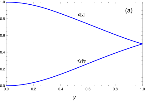
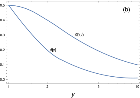
Figure 14: The suppression factors $\eta(y)/y$ and $\delta(y)$ as a function of $y\equiv\Delta M_{N}/\Gamma_{N}$: (a) for $y<1$ (on the linear $y$ scale); (b) for $1<y<10$ (on the logarithmic $y$ scale).

Branching ratios of experimental significance here can be defined by dividing the expressions $S_{\mp}(M)$, Equations (73) and (75) and (76), by the corresponding sum of total decay widths $[\Gamma(M^{+}\to{\rm all})+\Gamma(M^{-}\to{\rm all})]$, which is practically equal to $2\Gamma(M^{\pm}\to{\rm all})$

$${\rm Br}_{+}(M) \equiv \frac{S_{+}(M)}{2\Gamma(M^{\pm}\to{\rm all})}\$$ (88a)

$${\rm Br}_{-}(M) \equiv {\cal A}_{\rm CP}(M){\rm Br}_{+}(M)=\frac{S_{-}(M)}{2\Gamma(M^{\pm}\to{\rm all})}$$ (88b)

If employing the canonical (independent of mixing) branching ratio ${\overline{\rm Br}}(y_{N};y_{\ell_{1}},y_{\ell_{2}},y^{\prime})\equiv{\overline{\rm Br}}(DD^{*})$ defined in Equation (20) of Section II.1, and its $CC^{*}$ analog, ${\overline{\rm Br}}(CC^{*})\equiv{\overline{\rm Br}}(y_{N};y_{\ell_{2}},y_{\ell_{1}},y^{\prime})$, then it turns out that the branching ratios ${\rm Br}_{\pm}(M)$ of Equation (88) can be rewritten in terms of ${\overline{\rm Br}}$, of the heavy-light mixing parameters $|B_{\ell N_{j}}|$ and ${\widetilde{\cal K}}_{j}=\sum_{\ell}{\cal N}_{\ell N_{j}}|B_{\ell N_{j}}|^{2}$, of function $\eta(y)/y=y/(y^{2}+1)$ and the overlap function $\delta(y)$ tabulated in Table 4

$${\rm Br}_{+}(M)\equiv\frac{\Gamma(M^{-}\to\ell_{1}^{-}\ell_{2}^{-}M^{{}^{\prime}+})+\Gamma(M^{+}\to\ell_{1}^{+}\ell_{2}^{+}M^{{}^{\prime}-})}{2\Gamma(M^{\pm}\to{\rm all})}=2(2-\delta_{\ell_{1}\ell_{2}}){\Bigg{[}}\sum_{j=1}^{2}\frac{|B_{\ell_{1}N_{j}}|^{2}|B_{\ell_{2}N_{j}}|^{2}}{{\widetilde{\cal K}}_{j}}$$ (89a)

$$+4\delta(y)\frac{|B_{\ell_{1}N_{1}}||B_{\ell_{2}N_{1}}||B_{\ell_{1}N_{2}}||B_{\ell_{2}N_{2}}|}{({\widetilde{\cal K}}_{1}+{\widetilde{\cal K}}_{2})}\cos\theta_{21}{\Bigg{]}}\left({\overline{\rm Br}}(DD^{*})+{\overline{\rm Br}}(CC^{*})\right)$$

$${\rm Br}_{-}(M)\equiv{\cal A}_{\rm CP}(M){\rm Br}_{+}(M)\equiv\frac{\Gamma(M^{-}\to\ell_{1}^{-}\ell_{2}^{-}M^{{}^{\prime}+})-\Gamma(M^{+}\to\ell_{1}^{+}\ell_{2}^{+}M^{{}^{\prime}-})}{2\Gamma(M^{\pm}\to{\rm all})}$$ (89b)

$$= 8(2-\delta_{\ell_{1}\ell_{2}})\frac{|B_{\ell_{1}N_{1}}||B_{\ell_{2}N_{1}}||B_{\ell_{1}N_{2}}||B_{\ell_{2}N_{2}}|}{({\widetilde{\cal K}}_{1}+{\widetilde{\cal K}}_{2})}\;\sin\theta_{21}\;\frac{\eta(y)}{y}\left({\overline{\rm Br}}(DD^{*})+{\overline{\rm Br}}(CC^{*})\right)$$

This leads to an expression for the CP violation parameter ${\cal A}_{\rm CP}(M)$ defined in Equation (68), which now involves only the heavy-light mixing parameters $|B_{\ell N_{j}}|$ and ${\widetilde{\cal K}}_{j}$ [cf. Equation (18)], the function $\eta(y)/y=y/(y^{2}+1)$, where $y\equiv\Delta M_{N}/\Gamma_{N}$, and the overlap function $\delta(y)$ tabulated in Table 4:

$${\cal A}_{\rm CP}(M)\equiv\frac{{\rm Br}_{-}(M)}{{\rm Br}_{+}(M)}\equiv\frac{\Gamma(M^{-}\to\ell_{1}^{-}\ell_{2}^{-}M^{{}^{\prime}+})-\Gamma(M^{+}\to\ell_{1}^{+}\ell_{2}^{+}M^{{}^{\prime}-})}{\Gamma(M^{-}\to\ell_{1}^{-}\ell_{2}^{-}M^{{}^{\prime}+})+\Gamma(M^{+}\to\ell_{1}^{+}\ell_{2}^{+}M^{{}^{\prime}-})}$$ (90a)

$$= \frac{4\sin\theta_{21}}{\left[\sum_{j=1}^{2}\frac{|B_{\ell_{1}N_{j}}|^{2}|B_{\ell_{2}N_{j}}|^{2}}{|B_{\ell_{1}N_{1}}||B_{\ell_{2}N_{1}}||B_{\ell_{1}N_{2}}||B_{\ell_{2}N_{2}}|}\frac{({\widetilde{\cal K}}_{1}+{\widetilde{\cal K}}_{2})}{{\widetilde{\cal K}}_{j}}+4\delta(y)\cos\theta_{21}\right]}\;\frac{y}{(y^{2}+1)}$$

$$= \frac{4\sin\theta_{21}}{\left\{\left[\kappa_{\ell_{1}}\kappa_{\ell_{2}}\left(1+\frac{{\widetilde{\cal K}}_{1}}{{\widetilde{\cal K}}_{2}}\right)+\frac{1}{\kappa_{\ell_{1}}\kappa_{\ell_{2}}}\left(1+\frac{{\widetilde{\cal K}}_{2}}{{\widetilde{\cal K}}_{1}}\right)\right]+4\delta(y)\cos\theta_{21}\right\}}\;\frac{y}{(y^{2}+1)}\$$ (90b)

In the usually considered case $\ell_{1}=\ell_{2}$ ($\equiv\ell$), i.e., when the considered decays are $M^{\pm}\to\ell^{\pm}\ell^{\pm}M^{{}^{\prime}\mp}$, the formulas (89) and (90) get simpler, because in such a case ${\overline{\rm Br}}(CC^{*})={\overline{\rm Br}}(DD^{*})\equiv{\overline{\rm Br}}$, and $B_{\ell_{2}N_{j}}=B_{\ell_{1}N_{j}}\equiv B_{\ell N_{j}}$, and $\kappa_{\ell_{2}}=\kappa_{\ell_{1}}=\kappa_{\ell}$

$${\rm Br}_{+}(M) = 4\left[\sum_{j=1}^{2}\frac{|B_{\ell N_{j}}|^{4}}{{\widetilde{\cal K}}_{j}}+4\delta(y)\frac{|B_{\ell N_{1}}|^{2}|B_{\ell N_{2}}|^{2}}{({\widetilde{\cal K}}_{1}+{\widetilde{\cal K}}_{2})}\cos\theta_{21}\right]{\overline{\rm Br}}\$$ (91a)

$${\rm Br}_{-}(M) \equiv {\cal A}_{\rm CP}(M){\rm Br}_{+}(M)=16\frac{|B_{\ell N_{1}}|^{2}|B_{\ell N_{2}}|^{2}}{({\widetilde{\cal K}}_{1}+{\widetilde{\cal K}}_{2})}\;\sin\theta_{21}\;\frac{\eta(y)}{y}{\overline{\rm Br}}\$$ (91b)

$${\cal A}_{\rm CP}(M) = \frac{4\sin\theta_{21}}{\left\{\left[\kappa_{\ell}^{2}\left(1+\frac{{\widetilde{\cal K}}_{1}}{{\widetilde{\cal K}}_{2}}\right)+\frac{1}{\kappa_{\ell}^{2}}\left(1+\frac{{\widetilde{\cal K}}_{2}}{{\widetilde{\cal K}}_{1}}\right)\right]+4\delta(y)\cos\theta_{21}\right\}}\;\frac{y}{(y^{2}+1)}\$$ (91c)

These formulas become even simpler if the absolute values of the heavy-light mixings of $N_{1}$ and $N_{2}$ are equal (but not their phases), i.e., when

$$|B_{\ell^{{}^{\prime}}N_{2}}|^{2}\approx|B_{\ell^{{}^{\prime}}N_{1}}|^{2}\equiv|B_{\ell^{{}^{\prime}}N}|^{2}\qquad(\ell^{{}^{\prime}}=e,\mu,\tau)$$ (92)

In such a case, we have all $\kappa_{\ell^{{}^{\prime}}}\approx 1$, and ${\widetilde{\cal K}}_{2}\approx{\widetilde{\cal K}}_{1}\equiv{\widetilde{\cal K}}$, and therefore the expressions (91) reduce to

$${\rm Br}_{+}(M) \approx 8\frac{|B_{\ell N}|^{4}}{{\widetilde{\cal K}}}{\overline{\rm Br}}\left(1+{\cal O}(\delta)\right)\$$ (93a)

$${\rm Br}_{-}(M) \equiv {\cal A}_{\rm CP}(M){\rm Br}_{+}(M)\approx 8\frac{|B_{\ell N}|^{4}}{{\widetilde{\cal K}}}\;\sin\theta_{21}\;\frac{\eta(y)}{y}{\overline{\rm Br}}\$$ (93b)

$${\cal A}_{\rm CP}(M) \approx \sin\theta_{21}\frac{y}{y^{2}+1}\left(1+{\cal O}(\delta)\right)\leq\frac{1}{2}\sin\theta_{21}\left(1+{\cal O}(\delta)\right)$$ (93c)

In these expressions, we assumed, in addition, that the $N_{1}$-$N_{2}$ overlap terms are small (${\cal O}(\delta)$).

In order to obtain the corresponding effective (true) branching ratios, we have to multiply the above branching ratios ${\rm Br}_{\pm}$ by the decay-within-the-detector probability $P_{N_{j}}\equiv{\overline{P}}_{N}{\widetilde{\cal K}}_{j}(L/1{\rm m})$, as in Section II.2 ($L$ is the length of the detector). Again, the complicated mixing dependence entailed in the parameters ${\widetilde{\cal K}}_{j}$ gets cancelled in this multiplication. When adopting the simplifying assumption Equation (92), i.e., the validity of Equations (93), we obtain the following effective branching ratio ${\rm Br}_{\rm eff}$ and the CP violation effective branching ratio ${\cal A}_{\rm CP}{\rm Br}_{\rm eff}$:

$${\rm Br}_{\rm eff}(M^{\pm}\to\ell^{\pm}\ell^{\pm}M^{{}^{\prime}\mp}) = P_{N}{\rm Br}_{+}(M)\approx\left[{\overline{P}}_{N}\left(\frac{L}{1{\rm m}}\right){\widetilde{\cal K}}\right]\left[8\frac{|B_{\ell N}|^{4}}{{\widetilde{\cal K}}}{\overline{\rm Br}}\right]$$ (94a)

$$= \left(\frac{L}{1{\rm m}}\right)8|B_{\ell N}|^{4}{\overline{P}}_{N}{\overline{\rm Br}}\equiv 2|B_{\ell N}|^{4}\left(\frac{L}{1{\rm m}}\right){\overline{\rm Br}}_{\rm eff}$$

$${\cal A}_{\rm CP}{\rm Br}_{\rm eff}(M^{\pm}\to\ell^{\pm}\ell^{\pm}M^{{}^{\prime}\mp}) = \sin\theta_{21}\frac{y}{y^{2}+1}\times 2|B_{\ell N}|^{4}\left(\frac{L}{1{\rm m}}\right){\overline{\rm Br}}_{\rm eff}$$ (94b)

$$\lesssim |B_{\ell N}|^{4}\left(\frac{L}{1{\rm m}}\right)\sin\theta_{21}{\overline{\rm Br}}_{\rm eff}$$

In these formulas, we used the canonical effective branching ratio ${\overline{\rm Br}}_{\rm eff}$ as defined via Equations (32) and (20) and depicted in Figures 4–7 as a function of $M_{N}$ ($\equiv M_{N_{1}}\approx M_{N_{2}}$). The values of the Lorentz factors in the lab system are taken to be $\gamma_{N}=2$ for both $N_{1}$ and $N_{2}$, keeping in mind that ${\overline{\rm Br}}_{\rm eff}$ scales as $1/\gamma_{N}$. We recall that $\theta_{21}=2(\phi_{\ell 2}-\phi_{\ell 1})=2({\rm arg}(B_{\ell N_{2}})-{\rm arg}(B_{\ell N_{1}}))$. We notice that on the right-hand side of Equation (94a) there is an additional factor two in comparison with Equation (31b) of Section II.2; this factor two comes from the fact that we now have contributions of two intermediate neutrinos $N_{1}$ and $N_{2}$, and we neglected the contributions from the $N_{1}$-$N_{2}$ overlap (${\cal O}(\delta)$).

As at the end of Section II.2, let us consider now as an illustrative example the decays $D_{s}^{\pm}\to\mu^{\pm}\mu^{\pm}\pi^{\mp}$. In addition, let us assume that $|B_{\mu N}|^{2}$ is the dominant mixing. In such a case, the estimate Equation (33) is still valid, and the CP-violating difference of the effective branching ratios, ${\cal A}_{\rm CP}{\rm Br}_{\rm eff}$, is obtained by comparison of Equations (94a) and (94b)

$${\cal A}_{\rm CP}{\rm Br}_{\rm eff}(D^{\pm}_{s}\to\mu^{\pm}\mu^{\pm}\pi^{\mp})\sim 10^{2}|B_{\mu N}|^{4}\sin\theta_{21}\frac{y}{y^{2}+1}{\Big{|}}_{y\equiv\Delta M_{N}/\Gamma_{N}}\lesssim 10^{2}|B_{\mu N}|^{4}\sin\theta_{21}$$ (95)

Since for $M_{N}\approx 1$ GeV we have at present $|B_{\mu N}|^{2}\lesssim 10^{-7}$, cf. Table 2, Equation (95) means that ${\cal A}_{\rm CP}{\rm Br}^{\rm(eff)}\lesssim 10^{-12}$ for such decays. As already mentioned at the end of Section II.2, the proposed CERN-SPS experiment CERN-SPS ; CERN-SPS2 could produce $D$ and $D_{s}$ mesons in numbers by several orders of magnitude higher than $10^{12}$, and production of the sterile Majorana neutrinos $N_{j}$ could be explored. Further, if there exist two almost degenerate sterile neutrinos of mass $M_{N}\sim 1$ GeV (this is so in the $\nu$MSM model nuMSM ; nuMSM2 ; Shapo ; Shapo2 ; Shapo3 ; Shapo4 ; Shapo5 ; Shapo6 ), such that $y\equiv\Delta M_{N}/\Gamma_{N}\sim 1$, then we would have $\eta(y)/y\equiv y/(y^{2}+1)\sim 1$. In such a case the estimate (95) would imply that the CP-violating difference of effective branching ratios, ${\cal A}_{\rm CP}{\rm Br}_{\rm(eff)}(D_{s})$, is of the same order as the effective branching ratio ${\rm Br}_{\rm(eff)}(D_{s})$ (if the phase difference $|\theta_{21}|\not\ll 1$). Therefore, if experiments can discover the mentioned $\nu$MSM-type Majorana neutrinos, they will possibly detect also CP violation effects coming from the Majorana neutrinos.

The case of $B_{c}^{\pm}\to\mu^{\pm}\mu^{\pm}\pi^{\mp}$ is similar to the case of $D_{s}^{\pm}\to\mu^{\pm}\mu^{\pm}\pi^{\mp}$ described above, cf. Equations (33) and (34) at the end of Section II.2. Therefore, Equation (95) is valid also for CP violation in such decays of $B_{c}^{\pm}$. For the relative advantages and disadvantages of $D_{s}^{\pm}$ and $B_{c}^{\pm}$ decays, we refer to the comments at the end of Section II.2.

IV.2 CP Violation in Pion Decays $\pi^{\pm}\to e^{\pm}e^{\pm}\mu^{\mp}\nu$

In this Section, we will only briefly outline the calculation of the CP violation asymmetry in the (LNC and LNV) semileptonic decays $\pi^{\pm}\to e^{\pm}e^{\pm}\mu^{\mp}\nu$ as described in Section III. We will assume the presence of at least two nearly degenerate sterile neutrinos $N_{j}$ ($j=1,2$) that can go on shell in the intermediate state, as in Section IV.1. The present Section is a similar extension of the analysis of the decays $\pi^{\pm}\to e^{\pm}e^{\pm}\nu$ of Section III to two sterile neutrinos. The results of the present Section are largely based on Ref. CKZ . Only few details will be presented here, for further details we refer to Ref. CKZ .

Similarly to the previous Section IV.1, the quantities relevant for the CP violation will be

$${\rm Br}_{\pi,\pm}^{\rm(X)} = \frac{S^{\rm(X)}_{\pm}(\pi)}{2\Gamma(\pi^{\pm}\to{\rm all})}\equiv\frac{\Gamma^{(\rm X)}(\pi^{-}\to e^{-}e^{-}\mu^{+}\nu)\pm\Gamma^{\rm(X)}(\pi^{+}\to e^{+}e^{+}\mu^{-}\nu)}{2\Gamma(\pi^{\pm}\to{\rm all})}\$$ (96a)

$${\cal A}^{\rm(X)}_{\pi,\rm CP} = \frac{{\rm Br}_{\pi,-}^{\rm(X)}}{{\rm Br}_{\pi,+}^{\rm(X)}}=\equiv\frac{\Gamma^{\rm(X)}(\pi^{-}\to e^{-}e^{-}\mu^{+}\nu)-\Gamma^{\rm(X)}(\pi^{+}\to e^{+}e^{+}\mu^{-}\nu)}{\Gamma^{\rm(X)}(\pi^{-}\to e^{-}e^{-}\mu^{+}\nu)+\Gamma^{\rm(X)}(\pi^{+}\to e^{+}e^{+}\mu^{-}\nu)}$$ (96b)

where X = LNC, LNV. The total branching ratios are ${\rm Br}_{\pm}={\rm Br}_{\pm}^{\rm(LNV)}+{\rm Br}_{\pm}^{\rm(LNC)}$ when $N_{j}$ are Majorana neutrinos, and ${\rm Br}_{\pm}={\rm Br}_{\pm}^{\rm(LNC)}$ when $N_{j}$ are Dirac neutrinos. We adopt the same conventions and the same notations as in the previous Section IV.1. In addition, since we have now LNV and LNC processes, we introduce the additional notations

$$\theta^{\rm(LNV)} = 2(\phi_{e2}-\phi_{e1})$$ (97a)

$$\theta^{\rm(LNC)} = (\phi_{e2}-\phi_{e1})-(\phi_{\mu 2}-\phi_{\mu 1})$$ (97b)

As in Section IV.1, the requirement that the quantities $\sin\theta^{\rm(X)}$ (here: X = LNV, LNC) be nonzero, and the requirement of the near degeneracy of the two neutrinos ($\Delta M_{N}\ll M_{N_{1}}\equiv M_{N}$) in conjunction with the expressions Equations (79)–(83) for ${\rm Im}(P_{1}(D)P_{2}(D)^{*})$, are needed in order that the CP violation parameters ${\cal A}^{\rm(X)}_{\pi,\rm CP}\not=0$ acquire nonnegligible values. Analysis similar to that of the previous Section IV.1 (but algebraically more complicated) leads then to the results for the quantities defined in Equations (96). More specifically, the results for the Dirac case, ${\rm Br}_{\pi,+}^{\rm(Dir.)}\equiv{\rm Br}_{\pi,+}^{\rm(LNC)}$ and ${\cal A}^{\rm(Dir.)}_{\pi,\rm CP}\equiv{\cal A}^{\rm(LNC)}_{\pi,\rm CP}$, are the following:

$${\rm Br}_{\pi,+}^{\rm(Dir.)} \equiv \frac{\Gamma^{\rm(LNC)}(\pi^{-}\to e^{-}e^{-}\mu^{+}\nu)+\Gamma^{\rm(LNC)}(\pi^{+}\to e^{+}e^{+}\mu^{-}\nu)}{2\Gamma(\pi^{\pm}\to{\rm all})}$$ (98a)

$$= {\bigg{[}}\sum_{j=1}^{2}\frac{|B_{eN_{j}}|^{2}|B_{\mu N_{j}}|^{2}}{{\widetilde{\cal K}}_{j}}+4\delta(y)\frac{|B_{eN_{1}}||B_{eN_{2}}||B_{\mu N_{1}}||B_{\mu N_{2}}|}{({\widetilde{\cal K}}_{1}+{\widetilde{\cal K}}_{2})}\cos\theta^{\rm(LNC)}{\bigg{]}}{\overline{\rm Br}}_{\pi}\$$

$${\cal A}_{\pi,\rm CP}^{\rm(Dir.)} \equiv \frac{\Gamma^{\rm(LNC)}(\pi^{-}\to e^{-}e^{-}\mu^{+}\nu)-\Gamma^{\rm(LNC)}(\pi^{+}\to e^{+}e^{+}\mu^{-}\nu)}{\Gamma^{\rm(LNC)}(\pi^{-}\to e^{-}e^{-}\mu^{+}\nu)+\Gamma^{\rm(LNC)}(\pi^{+}\to e^{+}e^{+}\mu^{-}\nu)}$$ (98b)

$$= \frac{4\sin\theta^{\rm(LNC)}}{\left[\frac{|B_{eN_{1}}|}{|B_{eN_{2}}|}\frac{|B_{\mu N_{1}}|}{|B_{\mu N_{2}}|}\left(1+\frac{{\widetilde{\cal K}}_{2}}{{\widetilde{\cal K}}_{1}}\right)+\frac{|B_{eN_{2}}|}{|B_{eN_{1}}|}\frac{|B_{\mu N_{2}}|}{|B_{\mu N_{1}}|}\left(1+\frac{{\widetilde{\cal K}}_{1}}{{\widetilde{\cal K}}_{2}}\right)+4\delta(y)\cos\theta^{\rm(LNC)}\right]}\;\frac{\eta(y)}{y}$$

The expression for the canonical quantity ${\overline{\rm Br}}_{\pi}$, appearing in Equation (98a), is given in Equation (53) in conjunction with the notation (46) in Section III.1 The results for the Majorana case, ${\rm Br}_{\pi,+}^{\rm(Maj.)}$ $\equiv{\rm Br}_{\pi,+}^{\rm(LNV)}+{\rm Br}_{\pi,+}^{\rm(LNC)}$ and ${\cal A}^{\rm(Maj.)}_{\pi,\rm CP}$ are the following:

$${\rm Br}_{\pi,+}^{\rm(Maj.)} \equiv \frac{\sum_{{\rm X}={\rm LNV,LNC}}\left(\Gamma^{\rm(X)}(\pi^{-}\to e^{-}e^{-}\mu^{+}\nu)+\Gamma^{\rm(X)}(\pi^{+}\to e^{+}e^{+}\mu^{-}\nu)\right)}{2\Gamma(\pi^{\pm}\to{\rm all})}$$ (99a)

$$= {\bigg{[}}\sum_{j=1}^{2}\frac{|B_{eN_{j}}|^{2}(|B_{eN_{j}}|^{2}+|B_{\mu N_{j}}|^{2})}{{\widetilde{\cal K}}_{j}}+4\delta(y)\frac{|B_{eN_{1}}||B_{eN_{2}}|}{({\widetilde{\cal K}}_{1}+{\widetilde{\cal K}}_{2})}$$

$$\times\left(|B_{eN_{1}}||B_{eN_{2}}|\cos\theta^{\rm(LNV)}+|B_{\mu N_{1}}||B_{\mu N_{2}}|\cos\theta^{\rm(LNC)}\right){\bigg{]}}{\overline{\rm Br}}_{\pi}\$$

$${\cal A}_{\pi,\rm CP}^{\rm(Maj.)} \equiv \frac{\sum_{{\rm X}={\rm LNV,LNC}}\left(\Gamma^{\rm(X)}(\pi^{-}\to e^{-}e^{-}\mu^{+}\nu)-\Gamma^{\rm(X)}(\pi^{+}\to e^{+}e^{+}\mu^{-}\nu)\right)}{\sum_{{\rm X}={\rm LNV,LNC}}\left(\Gamma^{\rm(X)}(\pi^{-}\to e^{-}e^{-}\mu^{+}\nu)+\Gamma^{\rm(X)}(\pi^{+}\to e^{+}e^{+}\mu^{-}\nu)\right)}$$ (99b)

$$= 4\left(\sin\theta^{\rm(LNV)}+\frac{|B_{\mu N_{1}}||B_{\mu N_{2}}|}{|B_{eN_{1}}||B_{eN_{2}}|}\sin\theta^{\rm(LNC)}\right)$$

$$\times{\Bigg{[}}\frac{(|B_{eN_{1}}|^{2}+|B_{\mu N_{1}}|^{2})}{|B_{eN_{2}}|^{2}}\left(1+\frac{{\widetilde{\cal K}}_{2}}{{\widetilde{\cal K}}_{1}}\right)+\frac{(|B_{eN_{2}}|^{2}+|B_{\mu N_{2}}|^{2})}{|B_{eN_{1}}|^{2}}\left(1+\frac{{\widetilde{\cal K}}_{1}}{{\widetilde{\cal K}}_{2}}\right)$$

$$+4\delta(y)\left(\cos\theta^{\rm(LNV)}+\frac{|B_{\mu N_{1}}||B_{\mu N_{2}}|}{|B_{eN_{1}}||B_{eN_{2}}|}\cos\theta^{\rm(LNC)}\right){\Bigg{]}}^{-1}\times\frac{\eta(y)}{y}\$$

The function $\eta(y)/y=y/(y^{2}+1)$ is the same as in Section IV.1 (with: $y\equiv\Delta M_{N}/\Gamma_{N}$). Even more so, numerical evaluations give for the $N_{1}$-$N_{2}$ overlap parameter $\delta(y)$ the same values as in the semileptonic decays of Section IV.1, cf. Table 4 and Figure 14 there.

If we assume that $|B_{\ell N_{2}}|\approx|B_{\ell N_{1}}|$ (for $\ell=e,\mu,\tau$), i.e., Equation (92), then we have ${\widetilde{\cal K}}_{1}\approx{\widetilde{\cal K}}_{2}\equiv{\widetilde{\cal K}}$, and the expressions for ${\cal A}_{\pi,\rm CP}$ simplify significantly

$${\cal A}_{\pi,\rm CP}^{\rm(Dir.)} = \frac{\sin\theta^{\rm(LNC)}}{\left(1+\delta(y)\cos\theta^{\rm(LNC)}\right)}\;\frac{\eta(y)}{y}=\sin\theta^{\rm(LNC)}\;\frac{\eta(y)}{y}\left(1+{\cal O}(\delta)\right)\$$ (100a)

$${\cal A}_{\pi,\rm CP}^{\rm(Maj.)} = \left(\frac{|B_{eN_{1}}|^{2}\sin\theta^{\rm(LNV)}+|B_{\mu N_{1}}|^{2}\sin\theta^{\rm(LNC)}}{|B_{eN_{1}}|^{2}+|B_{\mu N_{1}}|^{2}}\right)\frac{\eta(y)}{y}\left(1+{\cal O}(\delta)\right)\$$ (100b)

As in the case of semileptonic LNV decays of the previous Section IV.1, we see that the CP asymmetry parameter ${\cal A}_{\pi,\rm CP}$ can become appreciable and even of order one if the following two conditions are fulfilled simultaneously: (a) at least one of the angles $\theta^{\rm(X)}$ (X=LNC,LNV), defined in Equation (97), is appreciable; (b) the quantity $y\equiv\Delta M_{N}/\Gamma_{N}$ is $y\sim 1$ (near degeneracy). In such cases, the estimates for the effective (true) branching ratios ${\rm Br}_{\rm eff}^{\rm(X)}$ of Equations (63) and (64) would apply also to the CP-violating difference of effective branching ratios, ${\cal A}^{\rm(X)}_{\pi,\rm CP}{\rm Br}_{\rm eff}^{\rm(X)}$, where (X) = (Dir.),(Maj.).

V Conclusions

We have studied lepton number violating (LNV) semileptonic decays of charged pseudoscalar mesons, specifically $\pi^{\pm}$, $K^{\pm}$, $D^{\pm}$, $D_{s}^{\pm}$, $B^{\pm}$ and $B_{c}^{\pm}$, mediated by heavy neutrinos that can go on their mass shell.

We first presented the LNV semileptonic decays of charged Kaons and of the heavier mesons $D^{\pm}$, $D_{s}^{\pm}$, $B^{\pm}$ and $B_{c}^{\pm}$, in processes of the form $M^{\pm}\to\ell_{1}^{\pm}\ell_{2}^{\pm}M^{\prime\mp}$, mediated by on-shell massive neutrinos, where $M$ is the decaying meson and $M^{{}^{\prime}}$ a correspondingly lighter meson. We estimated the branching ratios as functions of the neutrino masses and mixing parameters, and found the scenarios where upper limits on the mixing parameters can be obtained. We also studied the effect on the observability of these decays due to the long neutrino lifetime, as the secondary decay vertex is likely to fall outside the detector for the range of neutrino masses that are relevant to these processes.

We then presented our corresponding study of charged pion decays, which in this case are purely leptonic since pions are the lightest mesons. Here we can have modes that conserve lepton number (LNC) as well as modes that violate lepton number (LNV), if the intermediate neutrinos are of Majorana type, while only the former modes occur if the intermediate neutrino is of Dirac type. However, these modes are not distinguished by the final state because the latter involves a standard neutrino, which is not experimentally observable. We find that it could be possible to discern the Majorana or Dirac nature of neutrinos if one is able to observe features in the final state distribution.

We finally explored the possibility of observing CP violation in the lepton sector using these meson decays mediated by massive neutrinos on shell. The CP signal in charged meson decays is the usual asymmetry between the decays of opposite charge mesons. We found that leptonic CP violation may show in semileptonic LNV decays of charged Kaons and charged B mesons, as well as in LNC and LNV decays of charged pions, depending on the mass of the intermediate neutrinos. It turns out that such CP violation becomes appreciable and possibly detectable if there are at least two heavy neutrinos almost degenerate in mass that can go on their mass shell. The neutrino mass splitting that gives maximal CP asymmetries is close to the neutrino decay width. This type scenario fits well into the so called neutrino minimal standard model ($\nu$MSM), which contains two almost degenerate Majorana neutrinos of mass near 1 GeV and another lighter neutrino of mass of order $10^{1}$ keV, a model that can explain simultaneously neutrino oscillations, the dark matter and the baryon asymmetry of the Universe.

Appendix

A.1. Explicit Formulas for Amplitudes of the $N_{j}$-mediated Decay $M^{\pm}\to\ell_{1}^{\pm}\ell_{2}^{\pm}M^{{}^{\prime}\mp}$

In this Appendix we provide, for completeness, formulas which are used in Sections II and IV.1. The formulas were presented in Ref. CKZ2 for the case of exchange of two different neutrinos $N_{1}$ and $N_{2}$. Here we present them in a slightly more general form, when the number of exchanged neutrinos is ${\cal N}$ ($N_{1},\ldots,N_{\cal N}$). In Section II the simpler case of ${\cal N}=1$ is taken, because such a case is representative enough for the consideration of the branching ratios there. On the other hand, the case ${\cal N}=2$ (or: ${\cal N}\geq 2$) is taken in Section IV, with two of the neutrinos ($N_{1}$, $N_{2}$) considered on-shell and almost degenerate, because in such a case significant CP violation effects can arise in the Majorana neutrino sector.

The amplitude squared $|{\cal T}(M^{\pm})|^{2}$ for the decay of Figure 1 appears in the expression Equation (3) for the decay width $\Gamma(M^{\pm}\to\ell_{1}^{\pm}\ell_{2}^{\pm}M^{{}^{\prime}\mp})$, and can be written in the form

$$|{\cal T}(M^{\pm})|^{2} = K^{2}\sum_{i=1}^{{\cal N}}\sum_{j=1}^{{\cal N}}k_{i}^{(\pm)}k_{j}^{(\pm)*}M_{N_{i}}M_{N_{j}}$$ (101)

$$\times{\big{[}}P_{i}(D)P_{j}(D)^{*}T_{\pm}(D)T_{\pm}(D)^{*}+P_{i}(C)P_{j}(C)^{*}T_{\pm}(C)T_{\pm}(C)^{*}$$

$$+\left(P_{i}(D)P_{j}(C)^{*}T_{\pm}(D)T_{\pm}(C)^{*}+P_{i}(C)P_{j}(D)^{*}T_{\pm}(C)T_{\pm}(D)^{*}\right){\big{]}}\$$

Here, $i,j=1,\ldots,{\cal N}$ are indices of contributions of the exchanges of intermediate neutrinos $N_{i},N_{j}$, and $X=D,C$ denote contributions of amplitudes of the direct and crossed channels, respectively, cf. Figure 1. Further, $k_{j}^{(\pm)}$ are the heavy-light mixing factors for $N_{j}$ defined in Equation (70); $P_{j}(X)$ ($j=1,2;X=D,C$) are the propagator functions of $N_{j}$ neutrino for the $D$ and $C$ channel, Equation (72). $K^{2}$ is the constant originating from the vertices and is given in Equation (9). These expressions appear in the normalized decay widths ${\widetilde{\Gamma}}_{\pm}(XY^{*})$ in Equation (7) when ${\cal N}=1$, and in ${\widetilde{\Gamma}}_{\pm}(XY^{*})_{ij}$ in Equation (71) when ${\cal N}\geq 2$. The quadratic expressions of $T_{\pm}(X)T_{\pm}(Y)^{*}$ in Equation (101) get simplified after summation over the final helicities of the leptons $\ell_{1}$ and $\ell_{2}$, and acquire the following form:

$$T_{\pm}(D)T_{\pm}(D)^{*} = 8{\big{[}}M_{M}^{2}M_{M^{\prime}}^{2}(p_{1}\cdot p_{2})-2M_{M}^{2}(p_{1}\cdot p_{M^{\prime}})(p_{2}\cdot p_{M^{\prime}})-2M_{M^{\prime}}^{2}(p_{1}\cdot p_{M})(p_{2}\cdot p_{M})$$ (102a)

$$+4(p_{1}\cdot p_{M})(p_{2}\cdot p_{M^{\prime}})(p_{M}\cdot p_{M^{\prime}}){\big{]}}\equiv T(D)T(D)^{*}\$$

$$T_{\pm}(C)T_{\pm}(C)^{*} = 8{\big{[}}M_{M}^{2}M_{M^{\prime}}^{2}(p_{1}\cdot p_{2})-2M_{M}^{2}(p_{1}\cdot p_{M^{\prime}})(p_{2}\cdot p_{M^{\prime}})-2M_{M^{\prime}}^{2}(p_{1}\cdot p_{M})(p_{2}\cdot p_{M})$$ (102b)

$$+4(p_{2}\cdot p_{M})(p_{1}\cdot p_{M^{\prime}})(p_{M}\cdot p_{M^{\prime}}){\big{]}}\equiv T(C)T(C)^{*}\$$

$$T_{\pm}(D)T_{\pm}(C)^{*} = 16{\Big{\{}}M_{M}^{2}(p_{1}\cdot p_{M^{\prime}})(p_{2}\cdot p_{M^{\prime}})+M_{M^{\prime}}^{2}(p_{1}\cdot p_{M})(p_{2}\cdot p_{M})-\frac{1}{2}M_{M}^{2}M_{M^{\prime}}^{2}(p_{1}\cdot p_{2})$$ (102c)

$$+(p_{M}\cdot p_{M^{\prime}})\left[-(p_{1}\cdot p_{M})(p_{2}\cdot p_{M^{\prime}})-(p_{2}\cdot p_{M})(p_{1}\cdot p_{M^{\prime}})+(p_{M}\cdot p_{M^{\prime}})(p_{1}\cdot p_{2})\right]$$

$$\mp i(p_{M}\cdot p_{M^{\prime}})\epsilon(p_{M},p_{1},p_{2},p_{M^{\prime}}){\Big{\}}}$$

$$T_{\pm}(C)T_{\pm}(D)^{*} = \left(T_{\pm}(D)T_{\pm}(C)^{*}\right)^{*}=T_{\mp}(D)T_{\mp}(C)^{*}=\left(T_{\mp}(C)T_{\mp}(D)^{*}\right)^{*}\$$ (102d)

where we used the notation

$$\epsilon(q_{1},q_{2},q_{3},q_{4})\equiv\epsilon^{\eta_{1}\eta_{2}\eta_{3}\eta_{4}}(q_{1})_{\eta_{1}}(q_{2})_{\eta_{2}}(q_{3})_{\eta_{3}}(q_{4})_{\eta_{4}}\$$ (103)

Here, $\epsilon^{\eta_{1}\eta_{2}\eta_{3}\eta_{4}}$ is the totally antisymmetric Levi-Civita tensor with the sign convention $\epsilon^{0123}=+1$.

The expression (102), together with the definition (71), imply for the normalized decay widths ${\widetilde{\Gamma}}_{\pm}(XY^{*})_{ij}$ of Equation (71) various symmetry relations, namely that ${\widetilde{\Gamma}}_{\pm}(DD^{*})$ and ${\widetilde{\Gamma}}_{\pm}(CC^{*})$ are self-adjoint (${\cal N}\times{\cal N}$) matrices, and that elements of the $D$-$C$ interference matrices ${\widetilde{\Gamma}}_{\pm}(CD^{*})$ and ${\widetilde{\Gamma}}_{\pm}(DC^{*})$ are simply related

$${\widetilde{\Gamma}}(DD^{*})_{ij} = \left({\widetilde{\Gamma}}(DD^{*})_{ji}\right)^{*}\ ,\qquad{\widetilde{\Gamma}}(CC^{*})_{ij}=\left({\widetilde{\Gamma}}(CC^{*})_{ji}\right)^{*}\ ,$$ (104a)

$${\widetilde{\Gamma}}_{\pm}(CD^{*})_{ij} = \left({\widetilde{\Gamma}}_{\pm}(DC^{*})_{ji}\right)^{*}\$$ (104b)

If the two final leptons are of the same flavor ($\ell_{1}=\ell_{2}$), one can use the property that the integration $d_{3}$ over the final particles is symmetric under exchange of $p_{1}$ and $p_{2}$ (because $M_{\ell_{1}}=M_{\ell_{2}}$), and we have the following additional symmetries:

$${\widetilde{\Gamma}}(DD^{*})_{ij} = {\widetilde{\Gamma}}(CC^{*})_{ij}\$$ (105a)

$${\widetilde{\Gamma}}_{\pm}(CD^{*})_{ij} = {\widetilde{\Gamma}}_{\pm}(DC^{*})_{ij}\$$ (105b)

and the ${\cal N}\times{\cal N}$ $D$-$C$ interference matrices ${\widetilde{\Gamma}}_{\pm}(CD^{*})$ become self-adjoint, too.

When ${\cal N}=1$, as in Section II, then we have in the case of $\ell_{1}=\ell_{2}$

$${\widetilde{\Gamma}}(DD^{*})={\widetilde{\Gamma}}(CC^{*})\quad({\cal N}=1\;{\rm and}\;\ell_{1}=\ell_{2})$$ (106)

A.2. Explicit Expression for the Function $Q$

The expression in Equations (12) and (78) is arrived at by using in the integration over the phase space of three final particles [Equations (3) and (4)], for the contribution of the $N$ neutrino, the identity

$$d_{3}\left(M(p_{M})\to\ell_{1}(p_{1})\ell_{2}(p_{2})M^{{}^{\prime}}(p_{M^{\prime}})\right)=$$ (107b)

$$d_{2}\left(M(p_{M})\to\ell_{1}(p_{1})N_{j}(p_{N})\right)dp_{N}^{2}d_{2}\left(N_{j}(p_{N})\to\ell_{2}(p_{2})M^{{}^{\prime}}(p_{M^{\prime}})\right)$$

$$d_{2}\left(M(p_{M})\to\ell_{2}(p_{2})N_{j}(p_{N})\right)dp_{N}^{2}d_{2}\left(N_{j}(p_{N})\to\ell_{1}(p_{1})M^{{}^{\prime}}(p_{M^{\prime}})\right)\$$

The first identity can be used for the $DD^{*}$ contribution (where $p_{N}=p_{M}-p_{1}$) and the second for the $CC^{*}$ contribution (where $p_{N}=p_{M}-p_{2}$). When one uses the identity (10) in the $DD^{*}$ contribution, and the analogous identity for the $CC^{*}$ contribution, the integration over $dp_{N}^{2}$ becomes trivial, and the $d_{2}$-type of integrations can be performed. Notice that this is equivalent to the factorization approach $\Gamma(M\to\ell_{1}N){\rm Br}(N\to\ell_{2}M^{{}^{\prime}})$, which holds when $N$ is on-shell. The obtained expression for ${\widetilde{\Gamma}}(DD^{*})$ is then the expression Equation (12) when ${\cal N}=1$ [Equation (78) when ${\cal N}\geq 2$] with the notations (14), where the obtained function $Q$ has the following form:

$$Q(y_{N};y_{\ell_{1}},y_{\ell_{2}},y^{\prime}) = {\bigg{\{}}\frac{1}{2}(y_{N}-y_{\ell_{1}})(y_{N}-y_{\ell_{2}})(1-y_{N}-y_{\ell_{1}})\left(1-\frac{y^{\prime}}{y_{N}}+\frac{y_{\ell_{2}}}{y_{N}}\right)$$ (108)

$$+{\big{[}}-y_{\ell_{1}}y_{\ell_{2}}(1+y^{\prime}+2y_{N}-y_{\ell_{1}}-y_{\ell_{2}})-y_{\ell_{1}}^{2}(y_{N}-y^{\prime})+y_{\ell_{2}}^{2}(1-y_{N})$$

$$+y_{\ell_{1}}(1+y_{N})(y_{N}-y^{\prime})-y_{\ell_{2}}(1-y_{N})(y_{N}+y^{\prime}){\big{]}}{\bigg{\}}}\$$

In the limit of massless charged leptons ($y_{\ell_{1}}=y_{\ell_{2}}=0$), this reduces to

$$Q(y_{N};0,0,y^{\prime})=\frac{1}{2}y_{N}^{2}(1-y_{N})\left(1-\frac{y^{\prime}}{y_{N}}\right)\$$ (109)

A.3. Calculation of the Total Decay Width of Neutrino $N$

In this Appendix, for completeness, we summarize the formulas needed for evaluation of the total decay width of a massive sterile neutrino $N$, cf. Equations (16)–(18) and Figure 2.

In Ref. Atre (Appendix C there), the formulas for the leptonic decay and semimesonic decay widths of a sterile neutrino $N$ have been obtained, for the masses $M_{N}\lesssim 1$ GeV. For higher values of the masses $M_{N}$, the calculation of the semileptonic decay widths becomes difficult because not all the resonances are known. Hence, for such masses the authors of Refs. HKS ; GKS proposed an inclusive approach, based on duality, for the calculation of the total contribution of the semileptonic decay width of $N$. It consists of representing the various (pseudoscalar and vector) meson channels by quark-antiquark channels. This approach was applied for $M_{N}\geq M_{\eta^{{}^{\prime}}}\approx 0.958$ GeV. Here we summarize the formulas given in Ref. HKS for the decay width channels (cf. also: Atre ). In some of these formulas, twice the decay width is given [$2\Gamma(N\to\ldots)$], signalling the fact that for each possible decay of Majorana neutrino in charged particles, there is an equally possible decay into charge conjugate channel (something not possible if $N$ is Dirac particle).

$$2\Gamma(N\to\ell^{-}\ell^{{}^{\prime}+}\nu_{\ell^{{}^{\prime}}}) = |B_{\ell N}|^{2}\frac{G_{F}^{2}}{96\pi^{3}}M_{N}^{5}I_{1}(x_{\ell},0,x_{\ell^{{}^{\prime}}})(1-\delta_{\ell\ell^{{}^{\prime}}})\ ,$$ (110a)

$$\Gamma(N\to\nu_{\ell}\ell^{{}^{\prime}-}\ell^{{}^{\prime}+}) = |B_{\ell N}|^{2}\frac{G_{F}^{2}}{96\pi^{3}}M_{N}^{5}{\big{[}}(g_{L}^{(\rm lept)}g_{R}^{(\rm lept)}+\delta_{\ell\ell^{{}^{\prime}}}g_{R}^{(\rm lept)})I_{2}(0,x_{\ell^{{}^{\prime}}},x_{\ell^{{}^{\prime}}})$$ (110b)

$$+\left((g_{L}^{(\rm lept)})^{2}+(g_{R}^{(\rm lept)})^{2}+\delta_{\ell\ell^{{}^{\prime}}}(1+2g_{L}^{(\rm lept)})\right)I_{1}(0,x_{\ell^{{}^{\prime}}},x_{\ell^{{}^{\prime}}}){\big{]}}$$

$$\sum_{\nu_{\ell}}\sum_{\nu^{{}^{\prime}}}\Gamma(N\to\nu_{\ell}\nu^{{}^{\prime}}{\bar{\nu}}^{{}^{\prime}}) = \sum_{{\ell}}|B_{\ell N}|^{2}\frac{G_{F}^{2}}{96\pi^{3}}M_{N}^{5}\$$ (110c)

In Equation (110a) factor $2$ was included because for Majorana neutrino $N$ both decays $N\to\ell^{-}\ell^{{}^{\prime}+}\nu_{\ell^{{}^{\prime}}}$ and $N\to\ell^{+}\ell^{{}^{\prime}-}\nu_{\ell^{{}^{\prime}}}$ contribute ($\ell\not=\ell^{{}^{\prime}}$).

When $M_{N}<M_{\eta^{{}^{\prime}}}\approx 0.968$ GeV, the following semimesonic decays contribute, which involve presudoscalar ($P$) and vector ($V$) mesons:

$$2\Gamma(N\to\ell^{-}P^{+}) = |B_{\ell N}|^{2}\frac{G_{F}^{2}}{8\pi}M_{N}^{3}f_{P}^{2}|V_{P}|^{2}F_{P}(x_{\ell},x_{P})\$$ (111a)

$$\Gamma(N\to\nu_{\ell}P^{0}) = |B_{\ell N}|^{2}\frac{G_{F}^{2}}{64\pi}M_{N}^{3}f_{P}^{2}(1-x_{P}^{2})^{2}\$$ (111b)

$$2\Gamma(N\to\ell^{-}V^{+}) = |B_{\ell N}|^{2}\frac{G_{F}^{2}}{8\pi}M_{N}^{3}f_{V}^{2}|V_{V}|^{2}F_{V}(x_{\ell},x_{V})\$$ (111c)

$$\Gamma(N\to\nu_{\ell}V^{0}) = |B_{\ell N}|^{2}\frac{G_{F}^{2}}{2\pi}M_{N}^{3}f_{V}^{2}\kappa_{V}^{2}(1-x_{V}^{2})^{2}(1+2x_{V}^{2})\$$ (111d)

where factor $2$ in the charged meson channels appears because both decays $N\to\ell^{-}M^{{}^{\prime}+}$ and $N\to\ell^{+}M^{{}^{\prime}-}$ contribute ($M^{{}^{\prime}}=P,V$) if $N$ is Majorana. The factors $V_{P}$ and $V_{V}$ are the CKM matrix elements involving the valence quarks of the mesons; and $f_{P}$ and $f_{V}$ are the corresponding decay constants, whose values are given, e.g., in Table 1 in Ref. HKS . The pseudoscalar mesons which contribute here are: $P^{\pm}=\pi^{\pm},K^{\pm}$; $P^{0}=\pi^{0},K^{0},{\bar{K}}^{0},\eta$. The vector mesons which contribute are: $V^{\pm}=\rho^{\pm},K^{*\pm}$; $V^{0}=\rho^{0},\omega,K^{*0},{\bar{K}}^{*0}$. If $M_{N}\geq M_{\eta^{{}^{\prime}}}$ ($=$0.9578 GeV), due to duality the (many) semimesonic decay modes are represented by the following quark-antiquark decay modes HKS :

$$2\Gamma(N\to\ell^{-}U{\bar{D}}) = |B_{\ell N}|^{2}\frac{G_{F}^{2}}{32\pi^{3}}M_{N}^{5}|V_{UD}|^{2}I_{1}(x_{\ell},x_{U},x_{D})\$$ (112a)

$$\Gamma(N\to\nu_{\ell}q{\bar{q}}) = |B_{\ell N}|^{2}\frac{G_{F}^{2}}{32\pi^{3}}M_{N}^{5}\left[g_{L}^{(q)}g_{R}^{(q)}I_{2}(0,x_{q},x_{q})\!+\!\left((g_{L}^{(q)})^{2}\!+\!(g_{R}^{(q)})^{2}\right)I_{1}(0,x_{q},x_{q})\right]\$$ (112b)

In the formulas (110)–(112) the notations $x_{Y}\equiv M_{Y}/M_{N}$ ($Y=\ell,\nu_{\ell},P,V,q$) are used; and in Equation (112) we denoted: $U=u,c$; $D=d,s,b$; $q=u,d,c,s,b$. The values of quark masses which we used in our evaluations are: $M_{u}=M_{d}=3.5$ MeV; $M_{s}=105$ MeV; $M_{c}=1.27$ GeV; $M_{b}=4.2$ GeV.

We note that in the evaluation of the total decay width $\Gamma_{N}$, the expressions (112a) and (112b) should be added when $N$ is Majorana; if $N$ is Dirac, the same summation should be taken, but the expressions (112a) should be multiplied by $1/2$. The same approach is valid also in the case of summation of expressions (110) and (111).

In Equations (110b) and (112b) there appear the following SM neutral current couplings:

$$g_{L}^{(\rm lept)} = -\frac{1}{2}+\sin^{2}\theta_{W}\ ,\quad g_{R}^{(\rm lept)}=\sin^{2}\theta_{W}\$$ (113a)

$$g_{L}^{(U)} = \frac{1}{2}-\frac{2}{3}\sin^{2}\theta_{W}\ ,\quad g_{R}^{(U)}=-\frac{2}{3}\sin^{2}\theta_{W}\$$ (113b)

$$g_{L}^{(D)} = -\frac{1}{2}+\frac{1}{3}\sin^{2}\theta_{W}\ ,\quad g_{R}^{(U)}=\frac{1}{3}\sin^{2}\theta_{W}\$$ (113c)

Further, the neutral current couplings $\kappa_{V}$ of the neutral vector mesons in Equation (111d) are

$$\kappa_{V} = \frac{1}{3}\sin^{2}\theta_{W}\quad(V=\rho^{0},\omega)\$$ (114a)

$$\kappa_{V} = -\frac{1}{4}+\frac{1}{3}\sin^{2}\theta_{W}\quad(V=K^{*0},{\bar{K}}^{*0})\$$ (114b)

The following kinematical expressions $I_{1}$, $I_{2}$, $F_{P}$ and $F_{V}$ were used:

$$I_{1}(x,y,z) = 12\int_{(x+y)^{2}}^{(1-z)^{2}}\;\frac{ds}{s}(s-x^{2}-y^{2})(1+z^{2}-s)\lambda^{1/2}(s,x^{2},y^{2})\lambda^{1/2}(1,s,z^{2})\$$ (115a)

$$I_{2}(x,y,z) = 24yz\int_{(y+z)^{2}}^{(1-x)^{2}}\;\frac{ds}{s}(1+x^{2}-s)\lambda^{1/2}(s,y^{2},z^{2})\lambda^{1/2}(1,s,x^{2})\$$ (115b)

$$F_{P}(x,y) = \lambda^{1/2}(1,x^{2},y^{2})\left[(1+x^{2})(1+x^{2}-y^{2})-4x^{2}\right]\$$ (115c)

$$F_{V}(x,y) = \lambda^{1/2}(1,x^{2},y^{2})\left[(1-x^{2})^{2}+(1+x^{2})y^{2}-2y^{4}\right]\$$ (115d)

with $\lambda$ function defined in Equation (46a). These formulas allow us to obtain the total decay width $\Gamma(N\to{\rm all})$ as a function of $M_{N}$. Using these formulas, we evaluated the coefficients ${\cal N}_{\ell N}$, appearing in Equation (18) at the mixing terms $|B_{\ell N}|^{2}$, and presented them in Figure 2 as a function of $M_{N}$ for the cases of Majorana and Dirac neutrino $N$. One may notice a small kink in the curves of Figure 2 at $M_{N}=M_{\eta^{{}^{\prime}}}$ ($=$0.9578 GeV). This kink appears because at $M_{N}\geq M_{\eta^{{}^{\prime}}}$ the use of duality is made (the replacement of the semileptonic decay channel contributions by the quark-antiquark channel contributions). We can see that the duality works quite well at $M_{N}\geq M_{\eta^{{}^{\prime}}}$, with the possible exception for the case $\ell=\tau$ because $\tau$ lepton has a large mass.

A.4. Explicit Amplitudes for $N_{j}$-Mediated Decays $\pi^{\pm}\to e^{\pm}e^{\pm}\mu^{\mp}\nu$

In this Appendix we summarize, for completeness, formulas needed in Sections III and IV.2. These formulas were derived and presented in Ref. CKZ , for the case of exchange of two different neutrinos $N_{1}$ and $N_{2}$. Here we summarize them in a slightly more general form, for the case of ${\cal N}$ different neutrinos $N_{j}$ ($j=1,\ldots,{\cal N}$). In Section III the simpler case ${\cal N}=1$ is taken, as it is sufficiently representative for the branching ratios considered there. In Section IV the case ${\cal N}=2$ (or: ${\cal N}\geq 2$) is considered, with two (on-shell) neutrinos $N_{1}$ and $N_{2}$ almost degenerate, as in such a case significant CP violation effects can occur in the neutrino sector.

The squared amplitude $|{\cal T}_{\pi,\pm}^{\rm(X)}|^{2}$ for the $N_{j}$-mediated leptonic decays of neutrinos, appearing, for example, in Equation (36) (where X = LNC, LNV), is a combination of contributions from the two channels $D$ (direct) and $C$ (crossed) (cf. Figures 8 and 9), and, in general, of the contributions of ${\cal N}$ neutrinos $N_{j}$

$$|{\cal T}_{\pi,\pm}^{(X)}|^{2}=K_{\pi}^{2}\sum_{i=1}^{{\cal N}}\sum_{j=1}^{{\cal N}}k_{i,\pm}^{(X)*}k_{j,\pm}^{(X)}$$ (116)

$$\times{\bigg{[}}P_{i}^{(X)}(D)P_{j}^{(X)}(D)^{*}T_{{\pi},\pm}^{(X)}(DD^{*})+P_{i}^{(X)}(C)P_{j}^{(X)}(C)^{*}T_{{\pi},\pm}^{(X)}(CC^{*})$$

$$+\left(P_{i}^{(X)}(D)P_{j}^{(X)}(C)^{*}T_{{\pi},\pm}^{(X)}(DC^{*})+P_{i}^{(X)}(C)P_{j}^{(X)}(D)^{*}T_{{\pi},\pm}^{(X)}(CD^{*})\right){\bigg{]}}\$$

The constant $K_{\pi}^{2}$ is given in Equation (42), and the mixing factors $k_{j,\pm}^{(X)}$ are

$$k_{j,+}^{{\rm(LNV)}}=B_{eN_{j}}^{2}\ ,\qquad k_{j,+}^{{\rm(LNC)}}=B_{eN_{j}}B^{*}_{\mu N_{j}}\ ,\qquad k_{j,-}^{(X)}=\left(k_{j,+}^{(X)}\right)^{*}\$$ (117)

In the case of ${\cal N}=1$, these coefficients are in Equation (39). $P_{j}^{(X)}(Y)$ are the $N_{j}$-propagator functions [when ${\cal N}=1$: $N$-propagator functions of Equation (41)] of the direct and crossed channels ($Y=D,C$).

Explicit expressions for the direct ($DD^{*}$), crossed ($CC^{*}$) and direct-crossed interference ($DC^{*}$ and $CD^{*}$) terms [$T_{{\pi},\pm}^{\rm(X)}(DD^{*})$, $T_{{\pi},\pm}^{\rm(X)}(CC^{*})$, $T_{{\pi},\pm}^{\rm(X)}(DC^{*})$, $T_{{\pi},\pm}^{(X)}(CD^{*})$], appearing in Equations (116), get simplified when summed over the helicities of all the final leptons. In the case of the X = LNV processes (cf. Figure 9) they acquire the following form:

$$T_{{\pi},\pm}^{\rm(LNV)}(DD^{*}) = 256(p_{2}\cdot p_{\nu})\left[-M_{\pi}^{2}(p_{1}\cdot p_{\mu})+2(p_{1}\cdot p_{\pi})(p_{\mu}\cdot p_{\pi})\right]\equiv T_{\pi}^{\rm(LNV)}(DD^{*})\ ,$$ (118a)

$$T_{{\pi},\pm}^{\rm(LNV)}(CC^{*}) = 256(p_{1}\cdot p_{\nu})\left[-M_{\pi}^{2}(p_{2}\cdot p_{\mu})+2(p_{2}\cdot p_{\pi})(p_{\mu}\cdot p_{\pi})\right]\equiv T_{\pi}^{\rm(LNV)}(CC^{*})\ ,$$ (118b)

$$T_{{\pi},\pm}^{\rm(LNV)}(DC^{*}) = 128{\bigg{\{}}(p_{1}\cdot p_{\nu})\left[M_{\pi}^{2}(p_{2}\cdot p_{\mu})-2(p_{2}\cdot p_{\pi})(p_{\mu}\cdot p_{\pi})\right]$$ (118c)

$$+(p_{2}\cdot p_{\nu})\left[M_{\pi}^{2}(p_{1}\cdot p_{\mu})-2(p_{1}\cdot p_{\pi})(p_{\mu}\cdot p_{\pi})\right]$$

$$-(p_{1}\cdot p_{2})\left[M_{\pi}^{2}(p_{\nu}\cdot p_{\mu})-2(p_{\nu}\cdot p_{\pi})(p_{\mu}\cdot p_{\pi})\right]{\bigg{\}}}$$

$$\mp i{\bigg{\{}}-(p_{1}\cdot p_{\pi})\epsilon(p_{2},p_{\nu},p_{\mu},p_{\pi})+(p_{2}\cdot p_{\pi})\epsilon(p_{1},p_{\nu},p_{\mu},p_{\pi})$$

$$-(p_{\nu}\cdot p_{\pi})\epsilon(p_{1},p_{2},p_{\mu},p_{\pi})-(p_{\mu}\cdot p_{\pi})\epsilon(p_{1},p_{2},p_{\nu},p_{\pi}){\bigg{\}}}\$$

$$T_{{\pi},\pm}^{\rm(LNV)}(CD^{*}) = \left(T_{{\pi},\pm}^{\rm(LNV)}(DC^{*})\right)^{*}=T_{{\pi},\mp}^{\rm(LNV)}(DC^{*})\$$ (118d)

where we used the notation Equation (103) for $\epsilon$.

In the case of X = LNC processes (cf. Figure 8), the expressions are

$$T_{{\pi},\pm}^{\rm(LNC)}(DD^{*}) = 256(p_{\mu}\cdot p_{\nu}){\bigg{[}}(p_{1}\cdot p_{2})\left(M_{\pi}^{4}-M_{\pi}^{2}M_{e}^{2}-4M_{\pi}^{2}(p_{1}\cdot p_{\pi})+4(p_{1}\cdot p_{\pi})^{2}\right)$$ (119a)

$$+2M_{e}^{2}(p_{2}\cdot p_{\pi})(M_{\pi}^{2}-p_{1}\cdot p_{\pi}){\bigg{]}}\equiv T_{\pi}^{\rm(LNC)}(DD^{*})\$$

$$T_{{\pi},\pm}^{\rm(LNC)}(CC^{*}) = 256(p_{\mu}\cdot p_{\nu}){\bigg{[}}(p_{1}\cdot p_{2})\left(M_{\pi}^{4}-M_{\pi}^{2}M_{e}^{2}-4M_{\pi}^{2}(p_{2}\cdot p_{\pi})+4(p_{2}\cdot p_{\pi})^{2}\right)$$ (119b)

$$+2M_{e}^{2}(p_{1}\cdot p_{\pi})(M_{\pi}^{2}-p_{2}\cdot p_{\pi}){\bigg{]}}\equiv T_{\pi}^{\rm(LNC)}(CC^{*})\$$

$$T_{{\pi},\pm}^{\rm(LNC)}(DC^{*}) = 256(p_{\mu}\cdot p_{\nu}){\bigg{[}}(p_{1}\cdot p_{2})(M_{\pi}^{2}-2p_{1}\cdot p_{\pi})(M_{\pi}^{2}-2p_{2}\cdot p_{\pi})$$

$$+M_{e}^{2}\left(-2(p_{1}\cdot p_{\pi})^{2}-2(p_{2}\cdot p_{\pi})^{2}+M_{\pi}^{2}(p_{1}+p_{2})\cdot p_{\pi}+M_{\pi}^{2}M_{e}^{2}\right){\bigg{]}}$$

$$\equiv T_{\pi}^{\rm(LNC)}(DC^{*})\ ,$$

$$T_{\pi}^{\rm(LNC)}(CD^{*}) = \left(T_{\pi}^{\rm(LNC)}(DC^{*})\right)^{*}\$$ (119d)

These expressions appear in the definition of the normalized (i.e., without explicit mixing dependence) decay width matrices ${\widetilde{\Gamma}}_{\pi,\pm}^{\rm(X)}(YZ^{*})_{ij}$ (X = LNV, LNC; $Y,Z=D,C$; $i,j=1,\ldots,{\cal N}$)

$${\widetilde{\Gamma}}_{\pi,\pm}^{\rm(X)}(YZ^{*})_{ij}=K^{2}\;\frac{1}{2!}\frac{1}{2M_{\pi}}\frac{1}{(2\pi)^{8}}\int d_{4}\;P_{i}^{\rm(X)}(Y)P_{j}^{\rm(X)}(Z)^{*}\;T_{\pm}^{(X)}(YZ^{*})\$$ (120)

where $P_{j}^{\rm(X)}$ are the propagator functions of neutrino $N_{j}$ (with mass $M_{N_{j}}$), cf. the definitions (41) written when ${\cal N}=1$. When ${\cal N}=1$, the definition (120) reduces to the definition (40) in Section III.1.

When we use the symmetry of the $d_{4}$ integration under the exchange $p_{1}\leftrightarrow p_{2}$ (we note: $M_{1}=M_{2}=M_{e}$ in our considered case), this leads to the following identities:

$${\widetilde{\Gamma}}_{\pi}^{(X)}(DD^{*})_{ij} = {\widetilde{\Gamma}}_{\pi}^{(X)}(CC^{*})_{ij}\ ,\quad{\widetilde{\Gamma}}_{\pi}^{(X)}(DD^{*})_{ji}=\left({\widetilde{\Gamma}}_{\pi}^{(X)}(DD^{*})_{ij}\right)^{*}\$$ (121a)

$${\widetilde{\Gamma}}_{{\pi},\pm}^{(X)}(CD^{*})_{ij} = {\widetilde{\Gamma}}_{{\pi},\pm}^{(X)}(DC^{*})_{ij}=\left({\widetilde{\Gamma}}_{\pm}^{(X)}(CD^{*})_{ji}\right)^{*}\$$ (121b)

In the case of ${\cal N}=1$ this reduces simply to

$${\widetilde{\Gamma}}_{\pi}^{\rm(X)}(DD^{*})={\widetilde{\Gamma}}_{\pi}^{\rm(X)}(CC^{*})\$$ (122)

A.5. Explicit Expression for ${\widetilde{\Gamma}}_{\pi}^{\rm(X)}$ and $d{\widetilde{\Gamma}}_{\pi}^{\rm(X)}/dE_{\mu}$ for $\pi^{\pm}\to e^{\pm}e^{\pm}\mu^{\mp}\nu$ with On-Shell $N$

Equation (45) refers to the expression obtained by performing the integration (36) over the phase space of the four final particles [cf. Equation (37)], of the integrand written explicitly in Appendix 4. In the integration, the on-shellness (43) is assumed, which makes the integration over $p_{N}^{2}$ trivial. At the final stage of integration, the differential decay width $d{\widetilde{\Gamma}}^{\rm(X)}/dE_{\mu}$ over the muon energy $E_{\mu}$, in the rest frame of the $N$ neutrino, is performed. The expressions for $d{\widetilde{\Gamma}}^{\rm(X)}/dE_{\mu}$ were written in Refs. CDK ; CKZ , and we write them down here for completeness. In the case of X = LNV it is

$$\frac{d{\widetilde{\Gamma}}^{\rm(LNV)}(\pi^{\pm}\to e^{\pm}e^{\pm}\mu^{\mp}\nu)}{dE_{\mu}}$$ (123)

$$=\frac{K_{\pi}^{2}}{2(2\pi)^{4}}\frac{1}{\Gamma_{N}M_{\pi}^{3}}\lambda^{1/2}(M_{\pi}^{2},M_{N}^{2},M_{e}^{2})\times\left[M_{\pi}^{2}M_{N}^{2}-M_{N}^{4}+M_{e}^{2}(M_{\pi}^{2}+2M_{N}^{2}-M_{e}^{2})\right]$$

$$\times E_{\mu}\sqrt{E_{\mu}^{2}-M_{\mu}^{2}}\frac{(M_{N}^{2}-2M_{N}E_{\mu}+M_{\mu}^{2}-M_{e}^{2})^{2}}{(M_{N}^{2}-2M_{N}E_{\mu}+M_{\mu}^{2})}\quad\left(M_{\mu}\leq E_{\mu}\leq\frac{(M_{N}^{2}+M_{\mu}^{2}-M_{e}^{2})}{2M_{e}}\right).$$

The integration of this expression over $E_{\mu}$ can be performed explicitly (in Ref. CDK it was performed only in the limit $M_{e}=0$). The result is Equation (45) with notations (46), where the function ${\cal F}(x{\mu},x_{e})$ was obtained in Ref. CKZ . We write it down here again, for completeness.

$${\cal F}(x_{\mu},x_{e})={\Bigg{\{}}\lambda^{1/2}(1,x_{\mu},x_{e}){\big{[}}(1+x_{\mu})(1-8x_{\mu}+x_{\mu}^{2})-x_{e}(7-12x_{\mu}+7x_{\mu}^{2})$$ (124)

$$-7x_{e}^{2}(1+x_{\mu})+x_{e}^{3}{\big{]}}-24(1-x_{e}^{2})x_{\mu}^{2}\ln 2$$

$$+12{\bigg{[}}-x_{\mu}^{2}(1-x_{e}^{2})\ln x_{\mu}+(2x_{\mu}^{2}-x_{e}^{2}(1+x_{\mu}^{2}))\ln(1+x_{\mu}+\lambda^{1/2}(1,x_{\mu},x_{e})-x_{e})$$

$$+x_{e}^{2}(1-x_{\mu}^{2})\ln\left(\frac{(1-x_{\mu})^{2}+(1-x_{\mu})\lambda^{1/2}(1,x_{\mu},x_{e})-x_{e}(1+x_{\mu})}{x_{e}}\right){\bigg{]}}{\Bigg{\}}}\$$

We can obtain the LNV canonical differential decay width, according to Equation (54), from the normalized differential decay width Equation (123). For this, it turns out to be convenient to use the following identity:

$$\frac{2{\widetilde{\cal K}}}{\Gamma(\pi^{\pm}\to{\rm all})}\frac{K_{\pi}^{2}}{(2\pi)^{4}\Gamma_{N}M_{\pi}^{3}}=96\frac{1}{M_{N}^{5}M_{\mu}^{2}(M_{\pi}^{2}-M_{\mu}^{2})^{2}(1+\delta g_{\pi})}\$$ (125)

which is obtained by using Equations (42), (16) and (17) and (50). This then gives us

$$\frac{d{\overline{\rm Br}_{\pi}^{\rm(LNV)}}}{dE_{\mu}}\equiv 2\frac{{\widetilde{\cal K}}}{\Gamma_{\pi}}\frac{d{\widetilde{\Gamma}}^{\rm(LNV)}(\pi^{\pm}\to e^{\pm}e^{\pm}\mu^{\mp}\nu)}{dE_{\mu}}$$ (126)

$$=48\frac{1}{M_{N}^{5}M_{\mu}^{2}(M_{\pi}^{2}-M_{\mu}^{2})^{2}(1+\delta g_{\pi})}\lambda^{1/2}(M_{\pi}^{2},M_{N}^{2},M_{e}^{2})\times\left[M_{\pi}^{2}M_{N}^{2}-M_{N}^{4}+M_{e}^{2}(M_{\pi}^{2}+2M_{N}^{2}-M_{e}^{2})\right]$$

$$\times E_{\mu}\sqrt{E_{\mu}^{2}-M_{\mu}^{2}}\frac{(M_{N}^{2}-2M_{N}E_{\mu}+M_{\mu}^{2}-M_{e}^{2})^{2}}{(M_{N}^{2}-2M_{N}E_{\mu}+M_{\mu}^{2})}\qquad\left(M_{\mu}\leq E_{\mu}\leq(E_{\mu})_{\rm max}\right)$$

where

$$(E_{\mu})_{\rm max}=\frac{(M_{N}^{2}+M_{\mu}^{2}-M_{e}^{2})}{2M_{N}}$$ (127)

The LNC canonical differential decay width turns out to be

$$\frac{d{\overline{\rm Br}_{\pi}^{\rm(LNC)}}}{dE_{\mu}}\equiv 2\frac{{\widetilde{\cal K}}}{\Gamma_{\pi}}\frac{d{\widetilde{\Gamma}}^{\rm(LNC)}(\pi^{\pm}\to e^{\pm}e^{\pm}\mu^{\mp}\nu)}{dE_{\mu}}$$ (128)

$$=\frac{1}{M_{N}^{6}M_{\mu}^{2}(M_{\pi}^{2}-M_{\mu}^{2})^{2}(1+\delta g_{\pi})}\lambda^{1/2}(M_{\pi}^{2},M_{N}^{2},M_{e}^{2})\frac{1}{\left[M_{\mu}^{2}+M_{N}(-2E_{\mu}+M_{N})\right]^{3}}$$

$$\times{\bigg{\{}}8\sqrt{(E_{\mu}^{2}-M_{\mu}^{2})}M_{N}\left[(2E_{\mu}-M_{N})M_{N}-M_{\mu}^{2}+M_{e}^{2}\right]^{2}$$

$$\times\left[M_{\pi}^{2}M_{N}^{2}-M_{N}^{4}+M_{e}^{2}(M_{\pi}^{2}+2M_{N}^{2})-M_{e}^{4}\right]$$

$$\times{\Big{[}}8E_{\mu}^{3}M_{N}^{2}-2M_{\mu}^{2}M_{N}(M_{\mu}^{2}+M_{N}^{2}+2M_{e}^{2})-2E_{\mu}^{2}M_{N}\left(5(M_{\mu}^{2}+M_{N}^{2})+M_{e}^{2}\right)$$

$$+E_{\mu}\left(3M_{\mu}^{4}+10M_{\mu}^{2}M_{N}^{2}+3M_{N}^{4}+3M_{e}^{2}(M_{\mu}^{2}+M_{N}^{2})\right){\Big{]}}{\bigg{\}}}\qquad\left(M_{\mu}\leq E_{\mu}\leq(E_{\mu})_{\rm max}\right)$$

It turns out that, upon integration of this expression over $E_{\mu}$, we obtain the same result as in the X = LNV case, i.e., Equations (53c) with (46) and (124), or equivalently, Equations (45) with (46) and (124). We must add that we found a typographical error in Equation (A.16) of Ref. CDK , where $E_{\ell}^{2}$ must be replaced by $2E_{\ell}^{2}$, and in Equations (B.1c) and (B3) of Ref. CKZ , where $(E_{\mu})_{\rm max}$ should read $(M_{N_{j}}^{2}+M_{\mu}^{2}-M_{e}^{2})/(2M_{N})$.

In the limit $M_{e}=0$ (which is a good approximation), the canonical differential decay widths (126) and (128) get simplified

$$\frac{d{\overline{\rm Br}_{\pi}^{\rm(LNV)}}}{dE_{\mu}}{\Bigg{|}}_{M_{e}=0} = \frac{48(M_{\pi}^{2}-M_{N}^{2})^{2}}{M_{N}^{3}M_{\mu}^{2}(M_{\pi}^{2}-M_{\mu}^{2})^{2}}\sqrt{E_{\mu}^{2}-M_{\mu}^{2}}E_{\mu}(M_{N}^{2}-2M_{N}E_{\mu}+M_{\mu}^{2}),$$ (129a)

$$\frac{d{\overline{\rm Br}_{\pi}^{\rm(LNC)}}}{dE_{\mu}}{\Bigg{|}}_{M_{e}=0} = \frac{48(M_{\pi}^{2}-M_{N}^{2})^{2}}{M_{N}^{3}M_{\mu}^{2}(M_{\pi}^{2}-M_{\mu}^{2})^{2}}\sqrt{E_{\mu}^{2}-M_{\mu}^{2}}\left[\frac{1}{2}E_{\mu}(M_{N}^{2}+M_{\mu}^{2})-\frac{1}{3}M_{N}(2E_{\mu}^{2}+M_{\mu}^{2})\right]$$ (129b)

The full (integrated) canonical branching ratio in the $M_{e}=0$ limit is obtained by taking the $x_{e}=0$ limit of Equation (53c)

$${\overline{\rm Br}_{\pi}}{\big{|}}_{M_{e}=0}=\frac{1}{2}\frac{M_{N}^{2}}{M_{\mu}^{2}}\frac{(M_{\pi}^{2}-M_{N}^{2})^{2}}{(M_{\pi}^{2}-M_{\mu}^{2})^{2}}f\left(\frac{M_{\mu}^{2}}{M_{N}^{2}}\right)\$$ (130)

where the function $f$ is written in Equation (48).

A.6. Delta Function Approximation for the Imaginary Part of the Propagator Product

In this Appendix we investigate the expression for the imaginary part of the propagator product, ${\rm Im}(P_{1}(D)P_{2}(D)^{*})$, Equation (79a) of Section IV.1. For convenience we introduce in this Appendix the following simplified notations $x$, $M^{2}$, $\Delta$ and $\xi$:

$$x \equiv p_{N}^{2},\quad M^{2}\equiv M_{N_{1}}^{2}$$ (131a)

$$\Delta \equiv \Delta M_{N}^{2}\equiv M_{N_{2}}^{2}-M_{N_{1}}^{2}$$ (131b)

$$\Gamma_{N_{1}} = \xi\Gamma_{N},\quad\Gamma_{N_{2}}=(2-\xi)\Gamma_{N}$$ (131c)

We note that $\Delta>0$ by convention; and $0<\xi<2$. Further, $\Gamma_{N_{1}}+\Gamma_{N_{2}}=2\Gamma_{N}$, in accordance with the definition of $\Gamma_{N}$ Equation (82). Since we always have $\Gamma_{N_{j}}\ll M_{N_{j}}$ (the neutrinos $N_{j}$ are sterile), the relation (80) holds, i.e.,

$$\frac{\Gamma_{N_{j}}M_{N_{j}}}{(x-M_{N_{j}}^{2})^{2}+\Gamma_{N_{j}}^{2}M_{N_{j}}^{2}}=\pi\delta(x-M_{N_{j}}^{2})$$ (132)

We can write the right-hand side of Equation (79a) for ${\rm Im}(P_{1}(D)P_{2}(D)^{*})$ as

$${\rm Im}\left(P_{1}(D)P_{2}(D)^{*}\right)={\cal R}_{1}+{\cal R}_{2}$$ (133)

where ${\cal R}_{1}$ and ${\cal R}_{2}$ can be written, in our notation, as

$${\cal R}_{1} = \frac{(x-M^{2})(2-\xi)\Gamma_{N}\sqrt{M^{2}+\Delta}}{\left[(x-M^{2})^{2}+\xi^{2}\Gamma_{N}^{2}M^{2}\right]\left[(x-M^{2}-\Delta)^{2}+(2-\xi)^{2}\Gamma_{N}^{2}(M^{2}+\Delta)\right]}$$ (134a)

$$= \eta_{1}\times\frac{\pi}{\Delta}\delta(x-M^{2}-\Delta)$$ (134b)

$${\cal R}_{2} = -\frac{\xi\Gamma_{N}M(x-M^{2}-\Delta)}{\left[(x-M^{2})^{2}+\xi^{2}\Gamma_{N}^{2}M^{2}\right]\left[(x-M^{2}-\Delta)^{2}+(2-\xi)^{2}\Gamma_{N}^{2}(M^{2}+\Delta)\right]}$$ (134c)

$$= \eta_{2}\times\frac{\pi}{\Delta}\delta(x-M^{2})$$ (134d)

In Equations (134b) and (134d), the identity (132) was used, and we introduced two (dimensionless) parameters $\eta_{j}$ ($j=1,2$). We want to obtain these two parameters $\eta_{j}$. They can be obtained by integrating analytically the explicit expressions (134a) and (134c) for ${\cal R}_{j}(x)$ over $x$. For example, integration of ${\cal R}_{1}(x)$ gives

$$\int_{-\infty}^{+\infty}dx\frac{(x-M^{2})(2-\xi)\Gamma_{N}\sqrt{M^{2}+\Delta}}{\left[(x-M^{2})^{2}+\xi^{2}\Gamma_{N}^{2}M^{2}\right]\left[(x-M^{2}-\Delta)^{2}+(2-\xi)^{2}\Gamma_{N}^{2}(M^{2}+\Delta)\right]}=\frac{\pi\Delta}{(\Delta^{2}+4\Gamma_{N}^{2}M_{*}^{2})}$$ (135)

where

$$M_{*}^{2} = \frac{1}{2}M^{2}\left[\left(2-\xi(2-\xi)\right)+\xi(2-\xi)\sqrt{1+\Delta/M^{2}}\right]+\frac{1}{4}(2-\xi)^{2}\Delta$$ (136a)

$$= M^{2}\left[1+(1-\xi/2)\frac{\Delta}{M^{2}}+{\cal O}\left(\frac{\Delta^{2}}{M^{4}}\right)\right]$$ (136b)

Therefore, in the case of near degeneracy ($\Delta\ll M^{2}$) we have $M_{*}^{2}=M^{2}$. If we now use in the integration over $dx$ the expression (134b) instead, take into account $M_{*}^{2}=M^{2}$ in the case of near degeneracy, and compare with (135), we obtain the following expression for the parameter $\eta_{1}$ by comparison with (135):

$$\eta_{1}\frac{1}{\Delta} = \frac{\Delta}{(\Delta^{2}+4\Gamma_{N}^{2}M^{2})}\quad(\Delta\ll M^{2})$$ (137a)

$$\eta_{1} = \frac{y^{2}}{y^{2}+1}\quad\left(y\equiv\frac{\Delta}{(2M\Gamma_{N})},\;\Delta\ll M^{2}\right)$$ (137b)

where in Equation (137b) we use the usual notation in this paper $y\equiv(M_{N_{2}}-M_{N_{1}})/\Gamma_{N}=\Delta/(2M\Gamma_{N})$. Here we note that $\Delta\equiv(M_{N_{2}}^{2}-M_{N_{1}}^{2})=(M_{N_{2}}-M_{N_{1}})2M_{N_{1}}$ in the case of near degeneracy $\Delta\ll M^{2}\equiv M_{N_{1}}^{2}$.

Doing the same procedure with the quantity ${\cal R}_{2}$, we obtain for $\eta_{2}$ the very same result as for $\eta_{1}$

$$\eta_{1}=\eta_{2}=\frac{y^{2}}{y^{2}+1}\quad(\Delta\ll M^{2})$$ (138)

References

- (1) Racah, G. On the symmetry of particle and antiparticle. Nuovo Cim. 1937, 14, 322–328.
- (2) Furry, W.H. On transition probabilities in double beta-disintegration. Phys. Rev. 1939, 56, 1184–1193.
- (3) Primakoff, H.; Rosen, S.P. Double beta decay. Rep. Prog. Phys. 1959, 22, 121–166.
- (4) Primakoff, H.; Rosen, S.P. Nuclear double-beta decay and a new limit on lepton nonconservation. Phys. Rev. 1969, 184, 1925–1933.
- (5) Primakoff, H.; Rosen, S.P. Baryon number and lepton number conservation laws. Ann. Rev. Nucl. Part. Sci. 1981, 31, 145–192.
- (6) Schechter, J.; Valle, J.W.F. Neutrinoless double beta decay in theories. Phys. Rev. D 1982, 25, 2951–2954.
- (7) Doi, M.; Kotani, T.; Takasugi, E. Double beta decay and Majorana neutrino. Prog. Theor. Phys. Suppl. 1985, 83, 1–368.
- (8) Elliott, S.R.; Engel, J. Double beta decay. J. Phys. G 2004, 30, R183–R215.
- (9) Rodin, V.A.; Faessler, A.; Šimković, F.; Vogel, P. Assessment of uncertainties in QRPA -decay nuclear matrix elements. Nucl. Phys. A 2006, 766, 107–131.
- (10) Rodin, V.A.; Faessler, A.; Šimković, F.; Vogel, P. Erratum to: “Assessment of uncertainties in QRPA -decay nuclear matrix elements” [Nucl. Phys. A 766 (2006) 107]. Nucl. Phys. A 2007, 793, 213–215.
- (11) Keung, W.Y.; Senjanović, G. Majorana neutrinos and the production of the right-handed charged gauge boson. Phys. Rev. Lett. 1983, 50, 1427–1430.
- (12) Tello, V.; Nemevšek, M.; Nesti, F.; Senjanović, G.; Vissani, F. Left-right symmetry: From LHC to neutrinoless double beta decay. Phys. Rev. Lett. 2011, 106, doi:10.1103/PhysRevLett.106.151801.
- (13) Nemevšek, M.; Nesti, F.; Senjanović, G.; Tello, V. Neutrinoless double beta decay: Low left-right symmetry scale? Available online: http://arxiv.org/abs/1112.3061 (accessed on 27 April 2015).
- (14) Senjanović, G. Neutrino mass: From LHC to grand unification. Riv. Nuovo Cim. 2011, 34, 1–68.
- (15) Buchmüller, W.; Greub, C. Heavy Majorana neutrinos in electron-positron and electron-proton collisions. Nucl. Phys. B 1991, 363, 345–368.
- (16) Helo, J.; Hirsch, M.; Kovalenko, S. Heavy neutrino searches at the LHC with displaced vertices. Phys. Rev. D 2014, 89, doi:10.1103/PhysRevD.89.073005.
- (17) Kohda, M.; Sugiyama, M.; Tsumura, K. Lepton number violation at the LHC with leptoquark and diquark. Phys. Lett. B 2013, 718, 1436–1440.
- (18) Chen, C.Y.; Bhupal Dev, P.S. Multi-lepton collider signatures of heavy Dirac and Majorana neutrinos. Phys. Rev. D 2012, 85, doi:10.1103/PhysRevD.85.093018.
- (19) Chen, C.Y.; Bhupal Dev, P.S.; Mohapatra, R.N. Probing heavy-light neutrino mixing in Left-Right Seesaw models at the LHC. Phys. Rev. D 2013, 88, doi:10.1103/PhysRevD.88.033014.
- (20) Bhupal Dev, P.S.; Pilaftsis, A.; Yang, U.-K. New production mechanism for heavy neutrinos at the LHC. Phys. Rev. Lett. 2014, 112, 081801:1–081801:5.
- (21) Das, A.; Bhupal Dev, P.S.; Okada, N. Direct bounds on electroweak scale pseudo-Dirac neutrinos from TeV LHC data. Phys. Lett. B 2014, 735, 364–370.
- (22) Littenberg, L.S.; Shrock, R.E. Upper bounds on lepton number violating meson decays. Phys. Rev. Lett. 1992, 68, 443–446.
- (23) Littenberg, L.S.; Shrock, R.E. Implications of improved upper bounds on processes. Phys. Lett. B 2000, 491, 285–290.
- (24) Dib, C.; Gribanov, V.; Kovalenko, S.; Schmidt, I. K meson neutrinoless double muon decay as a probe of neutrino masses and mixings. Phys. Lett. B 2000, 493, 82–87.
- (25) Ali, A.; Borisov, A.V.; Zamorin, N.B. Majorana neutrinos and same sign dilepton production at LHC and in rare meson decays. Eur. Phys. J. C 2001, 21, 123–132.
- (26) Cvetič, G.; Dib, C.; Kang, S.K.; Kim, C.S. Probing Majorana neutrinos in rare and meson decays. Phys. Rev. D 2010, 82, doi:10.1103/PhysRevD.82.053010.
- (27) Ivanov, M.A.; Kovalenko, S.G. Hadronic structure aspects of decays. Phys. Rev. D 2005, 71, doi:10.1103/PhysRevD.71.053004.
- (28) De Gouvea, A.; Jenkins, J. A Survey of lepton number violation via effective operators. Phys. Rev. D 2008, 77, doi:10.1103/PhysRevD.77.013008.
- (29) Atre, A.; Han, T.; Pascoli, S.; Zhang, B. The Search for heavy Majorana neutrinos. JHEP 2009, 0905, doi:10.1088/1126-6708/2009/05/030. and references therein.
- (30) Helo, J.C.; Kovalenko, S.; Schmidt, I. Sterile neutrinos in lepton number and lepton flavor violating decays. Nucl. Phys. B 2011, 853, 80–104.
- (31) Quintero, N.; López Castro, G.; Delepine, D. Lepton number violation in top quark and neutral B meson decays. Phys. Rev. D 2011, 84, doi:10.1103/PhysRevD.84.096011.
- (32) Quintero, N.; López Castro, G.; Delepine, D. Erratum: Lepton number violation in top quark and neutral B meson decays [Phys. Rev. D 84, 096011 (2011)]. Phys. Rev. D 2012, 86, doi:10.1103/PhysRevD.86.079905.
- (33) López Castro, G.; Quintero, N. Bounding resonant Majorana neutrinos from four-body B and D decays. Phys. Rev. D 2013, 87, doi:10.1103/PhysRevD.87.077901.
- (34) Abada, A.; Teixeira, A.M.; Vicente, A.; Weiland, C. Sterile neutrinos in leptonic and semileptonic decays. JHEP 2014, 1402, doi:10.1007/JHEP02(2014)091.
- (35) Wang, Y.; Bao, S.S.; Li, Z.H.; Zhu, N.; Si, Z.G. Study Majorana neutrino contribution to B-meson semi-leptonic rare decays. Phys. Lett. B 2014, 736, 428–432.
- (36) Boyanovsky, D. Nearly degenerate heavy sterile neutrinos in cascade decay: Mixing and oscillations. Phys. Rev. D 2014, 90, doi:10.1103/PhysRevD.90.105024.
- (37) Cvetič, G.; Dib, C.; Kim, C.S. Probing Majorana neutrinos in rare decays. JHEP 2012, 1206, doi:10.1007/JHEP06(2012)149.
- (38) Cvetič, G.; Kim, C.S.; Zamora-Saá, J. CP violations in meson decay. J. Phys. G 2014, 41, doi:10.1088/0954-3899/41/7/075004.
- (39) Cvetič, G.; Kim, C.S.; Zamora-Saá, J. CP violation in lepton number violating semileptonic decays of . Phys. Rev. D 2014, 89, doi:10.1103/PhysRevD.89.093012.
- (40) Dib, C.O.; Campos, M.; Kim, C.S. CP Violation with Majorana neutrinos in K meson decays. JHEP 2015, 1502, doi:10.1007/JHEP02(2015)108.
- (41) Fukuda, Y.; et al. [Super-Kamiokande Collaboration]. Evidence for oscillation of atmospheric neutrinos. Phys. Rev. Lett. 1998, 81, 1562–1567.
- (42) Ahmad, Q.R.; et al. [SNO Collaboration]. Direct evidence for neutrino flavor transformation from neutral current interactions in the Sudbury Neutrino Observatory. Phys. Rev. Lett. 2002, 89, doi:10.1103/PhysRevLett.89.011301.
- (43) Lipari, P. CP violation effects and high-energy neutrinos. Phys. Rev. D 2001, 64, doi:10.1103/PhysRevD.64.033002.
- (44) Rahman, Z.; Dasgupta, A.; Adhikari, R. Non-standard interaction effect on CP violation in neutrino oscillation with super-beam. Available online: http://arxiv.org/abs/1210.2603 (accessed on 28 April 2015).
- (45) Rahman, Z.; Dasgupta, A.; Adhikari, R. Discovery reach of CP violation and non-standard interactions in low energy neutrino factory. Available online: http://arxiv.org/abs/1210.4801 (accessed on 28 April 2015).
- (46) Eguchi, K.; et al. [KamLAND Collaboration]. First results from KamLAND: Evidence for reactor anti-neutrino disappearance. Phys. Rev. Lett. 2003, 90, doi:10.1103/PhysRevLett.90.021802.
- (47) Planck Collaboration. Planck 2013 results. XVI. Cosmological parameters. Astron. Astrophys. 2014, 571, A16 (66pp.).
- (48) Minkowski, P. at a rate of one out of 1-billion muon decays? Phys. Lett. B 1977, 67, 421–428.
- (49) Gell-Mann, M.; Ramond, P.; Slansky, R. The Family Group in Grand Unified Theories. In Supergravity; van Nieuwenhuizen, P., Freedman, D.Z., Eds.; North-Holland: Amsterdam, The Netherlands, 1979.
- (50) Yanagida, T. Horizontal symmetry and masses of neutrinos. Prog. Theor. Phys. 1980, 64, 1103–1105.
- (51) Glashow, S.L. Quarks and Leptons; Lévy, M., Basdevant, J.-L., Speiser, D., Weyers, J., Gastmans, R., Jacob, M.; Eds.; Cargese, Plenum: New York, NY, USA, 1980.
- (52) Mohapatra, R.N.; Senjanović, G. Neutrino mass and spontaneous parity violation. Phys. Rev. Lett. 1980, 44, 912–915.
- (53) Wyler, D.; Wolfenstein, L. Massless neutrinos in left-right symmetric models. Nucl. Phys. B 1983, 218, 205–214.
- (54) Witten, E. Symmetry breaking patterns in superstring models. Nucl. Phys. B 1985, 258, 75–100.
- (55) Mohapatra, R.N.; Valle, J.W.F. Neutrino mass and baryon number nonconservation in superstring models. Phys. Rev. D 1986, 34, 1642–1645.
- (56) Malinsky, M.; Romao, J.C.; Valle, J.W.F. Novel supersymmetric seesaw mechanism. Phys. Rev. Lett. 2005, 95, 161801:1–161801:5.
- (57) Dev, P.S.B.; Mohapatra, R.N. TeV Scale Inverse Seesaw in SO(10) and Leptonic Non-Unitarity Effects. Phys. Rev. D 2010, 81, doi:10.1103/PhysRevD.81.013001.
- (58) Dev, P.S.B.; Pilaftsis, A. Minimal Radiative Neutrino Mass Mechanism for Inverse Seesaw Models. Phys. Rev. D 2012, 86, doi:10.1103/PhysRevD.86.113001.
- (59) Lee, C.H.; Dev, P.S.B.; Mohapatra, R.N. Natural TeV-scale left-right seesaw mechanism for neutrinos and experimental tests. Phys. Rev. D 2013, 88, doi:10.1103/PhysRevD.88.093010.
- (60) Asaka, T.; Blanchet, S.; Shaposhnikov, M. The MSM, dark matter and neutrino masses. Phys. Lett. B 2005, 631, 151–156.
- (61) Asaka, T.; Shaposhnikov, M. The MSM, dark matter and baryon asymmetry of the universe. Phys. Lett. B 2005, 620, 17–26.
- (62) He, X.G.; Oh, S.; Tandean, S.J.; Wen, C.C. Large mixing of light and heavy neutrinos in seesaw models and the LHC. Phys. Rev. D 2009, 80, doi:10.1103/PhysRevD.80.073012.
- (63) Del Aguila, F.; Aguilar-Saavedra, J.A.; de Blas, J.; Zralek, M. Looking for signals beyond the neutrino Standard Model. Acta Phys. Polon. B 2007, 38, 3339–3348.
- (64) Kersten, J.; Smirnov, A.Y. Right-handed neutrinos at CERN LHC and the mechanism of neutrino mass generation. Phys. Rev. D 2007, 76, doi:10.1103/PhysRevD.76.073005.
- (65) Ibarra, A.; Molinaro, E.; Petcov, S.T. TeV scale see-saw mechanisms of neutrino mass generation, the Majorana nature of the heavy singlet neutrinos and -Decay. JHEP 2010, 1009, 108–129.
- (66) Cabibbo, N. Time reversal violation in neutrino oscillation. Phys. Lett. B 1978, 72, 333–335.
- (67) Gorbunov, D.; Shaposhnikov, M. How to find neutral leptons of the MSM? JHEP 2007, 0710, doi:10.1088/1126-6708/2007/10/015.
- (68) Shaposhnikov, M. Is there a new physics between electroweak and Planck scales? Available online: http://arxiv.org/abs/0708.3550 (accessed on 28 April 2015).
- (69) Boyarsky, A.; Ruchayskiy, O.; Shaposhnikov, M. The role of sterile neutrinos in cosmology and astrophysics. Ann. Rev. Nucl. Part. Sci. 2009, 59, 191–214.
- (70) Shaposhnikov, M. Neutrino physics within and beyond the three flavour oscillation. J. Phys. Conf. Ser. 2013, 408, doi:10.1088/1742-6596/408/1/012015.
- (71) Canetti, L.; Drewes, M.; Shaposhnikov, M. Sterile neutrinos as the origin of dark and baryonic matter. Phys. Rev. Lett. 2013, 110, doi:10.1103/PhysRevLett.110.061801.
- (72) Canetti, L.; Drewes, M.; Frossard, T.; Shaposhnikov, M. Dark matter, baryogenesis and neutrino oscillations from right handed neutrinos. Phys. Rev. D 2013, 87, doi:10.1103/PhysRevD.87.093006.
- (73) Canetti, L.; Drewes, M.; Garbrecht, B. Probing leptogenesis with GeV-scale sterile neutrinos at LHCb and Belle II. Phys. Rev. D 2014, 90, doi:10.1103/PhysRevD.90.125005.
- (74) Drewes, M.; Garbrecht, B. Experimental and cosmological constraints on heavy neutrinos. Available online: http://arxiv.org/abs/1502.00477 (accessed on 28 April 2015).
- (75) Pilaftsis, A. CP violation and baryogenesis due to heavy Majorana neutrinos. Phys. Rev. D 1997, 56, 5431–5451.
- (76) Bray, S.; Lee, J.S.; Pilaftsis, A. Resonant CP violation due to heavy neutrinos at the LHC. Nucl. Phys. B 2007, 786, 95–118.
- (77) Akhmedov, E.; Kartavtsev, A.; Lindner, M.; Michaels, L.; Smirnov, J. Improving Electro-Weak Fits with TeV-scale Sterile Neutrinos. JHEP 2013, 1305, doi:10.1007/JHEP05(2013)081.
- (78) Qian, X.; Zhang, C.; Diwan, M.; Vogel, P. Unitarity Tests of the Neutrino Mixing Matrix. Available online: http://arxiv.org/abs/1308.5700 (accessed on 28 April 2015).
- (79) Basso, L.; Fischer, O.; van der Bij, J.J. Precision tests of unitarity in leptonic mixing. Europhys. Lett. 2014, 105, doi:10.1209/0295-5075/105/11001.
- (80) Bonivento, W.; Boyarsky, A.; Dijkstra, H.; Egede, U.; Ferro-Luzzi, M.; Goddard, B.; Golutvin, A.; Gorbunov, D.; Jacobsson, R.; Panman, J.; et al. Proposal to Search for Heavy Neutral Leptons at the SPS. Available online: http://arxiv.org/abs/1310.1762 (accessed on 28 April 2015).
- (81) Jacobson, R. Search for heavy neutral neutrinos at the SPS. Presented at High Energy Physics in the LHC Era, UTFSM, Valparaíso, Chile, 16–20 December 2014. Available online: https://indico.cern.ch/event/252857/contribution/215 (accessed on April 29, 2015)
- (82) Dib, C.O.; Kim, C.S. Remarks on the lifetime of sterile neutrinos and the effect on detection of rare meson decays . Phys. Rev. D 2014, 89, doi:10.1103/PhysRevD.89.077301.
- (83) Beneš, P.; Faessler, A.; Šimković, F.; Kovalenko, S. Sterile neutrinos in neutrinoless double beta decay. Phys. Rev. D 2005, 71, doi:10.1103/PhysRevD.71.077901.
- (84) Bélanger, G.; Boudjema, F.; London, D.; Nadeau, H. Inverse neutrinoless double beta decay revisited. Phys. Rev. D 1996, 53, 6292–6301.
- (85) London, D. Inverse neutrinoless double beta decay (and other processes). Available online: http://arxiv.org/abs/hep-ph/9907419 (accessed on 28 April 2015).
- (86) Kusenko, A.; Pascoli, S.; Semikoz, D. New bounds on MeV sterile neutrinos based on the accelerator and Super-Kamiokande results. JHEP 2005, 0511, doi:10.1088/1126-6708/2005/11/028.
- (87) WA66 Collaboration. Search for heavy neutrino decays in the BEBC beam dump experiment. Phys. Lett. B 1985, 160, 207–211.
- (88) NA3 Collaboration. Mass and lifetime limits on new longlived particles in interactions. Z. Phys. C 1986, 31, 21–32.
- (89) Bernardi, G.; Carugno, G.; Chauveau, J.; Dicarlo, F.; Dris, M.; Dumarchez, J.; Ferro-Luzzi, M.; Levy, J.-M.; Lukas, D.; Perreau, J.-M.; et al. Further limits on heavy neutrino couplings. Phys. Lett. B 1988, 203, 332–334.
- (90) FMMF Collaboration. Search for neutral weakly interacting massive particles in the Fermilab Tevatron wide band neutrino beam. Phys. Rev. D 1995, 52, doi:10.1103/PhysRevD.52.6.
- (91) NuTeV and E815 Collaborations. Search for neutral heavy leptons in a high-energy neutrino beam. Phys. Rev. Lett. 1999, 83, 4943–4946.
- (92) L3 Collaboration. Search for isosinglet neutral heavy leptons in Z0 decays. Phys. Lett. B 1992, 295, 371–382.
- (93) CHARM II Collaboration. Search for heavy isosinglet neutrinos. Phys. Lett. B 1995, 343, 453–458 [Phys. Lett. B 1995, 351, 387–392].
- (94) DELPHI Collaboration. Search for neutral heavy leptons produced in Z decays. Z. Phys. C 1997, 74, 57–71.
- (95) NOMAD Collaboration. Search for heavy neutrinos mixing with tau neutrinos. Phys. Lett. B 2001, 506, 27–38.
- (96) Orloff, J.; Rozanov, A.N.; Santoni, C. Limits on the mixing of tau neutrino to heavy neutrinos. Phys. Lett. B 2002, 550, 8–15.
- (97) Particle Data Group Collaboration. Review of Particle Physics. Chin. Phys. C 2014, 38, doi:10.1088/1674-1137/38/9/090001.
- (98) Cvetič, G.; Kim, C.S.; Wang, G.L.; Namgung, W. Decay constants of heavy meson of 0-state in relativistic Salpeter method. Phys. Lett. B 2004, 596, 84–89.
- (99) PIENU Collaboration. Search for massive neutrinos in the decay . Phys. Rev. D 2011, 84, doi:10.1103/PhysRevD.84.052002.
- (100) Yamazaki, T.; Ishikawa, T.; Akiba, Y.; Iwasaki, M.; Tanaka, K.H.; Ohtake, S.; Tamura, H.; Nakajima, M.; Yamanaka, T.; Arai, I.; et al. Search for Heavy Neutrinos in Kaon Decay. Conf. Proc. C 1984, 840719, 262–262.
- (101) Hayano, R.S.; Taniguchi, T.; Yamanaka, T.; Tanimori, T.; Enomoto, R.; Ishibashi, A.; Ishikawa, T.; Sato, S.; Fujii, T.; Yamazaki, T.; et al. Heavy neutrino search using decay. Phys. Rev. Lett. 1982, 49, doi:10.1103/PhysRevLett.49.1305.
- (102) Kusenko, A.; Pascoli, S.; Semikoz, D. New bounds on MeV sterile neutrinos based on the accelerator and Super-Kamiokande results. JHEP 2005, 0511, doi:10.1088/1126-6708/2005/11/028.
- (103) Orloff, J.; Rozanov, A.N.; Santoni, C. Limits on the mixing of tau neutrino to heavy neutrinos. Phys. Lett. B 2002, 550, 8–15.
- (104) Ruchayskiy, O.; Ivashko, A. Experimental bounds on sterile neutrino mixing angles. JHEP 2012, 1206, doi:10.1007/JHEP06(2012)100.
- (105) Deppisch, F.F.; Dev, P.S.B.; Pilaftsis, A. Neutrinos and Collider Physics. Available online: http://arxiv.org/abs/1502.06541 (accessed on 28 April 2015).
- (106) Project X and the Science of the Intensity Frontier. In Proceedings of the Project X Physics Workshop, Fermilab, USA, 9–10 November 2009. Available online: http://www.fnal.gov/projectx/pdfs/ProjectXwhitepaperJan.v2.pdf (accessed on April 29, 2015).
- (107) Geer, S. Private communication,, Fermilab, 2012 (sgeer@fnal.gov).
- (108) Pontecorvo, B. Inverse beta processes and nonconservation of lepton charge. Sov. Phys. JETP 1958, 7, 172–173 [Zh. Eksp. Teor. Fiz. 1957, 34, 247].
- (109) Neutrino experiments and the problem of conservation of leptonic charge. Sov. Phys. JETP 1968, 26, 984–988 [Zh. Eksp. Teor. Fiz. 1967, 53, 1717].
- (110) Maki, Z.; Nakagawa, M.; Sakata, S. Remarks on the unified model of elementary particles. Prog. Theor. Phys. 1962, 28, 870–880.
- (111) Bilenky, S. Introduction to the Physics of Massive and Mixed Neutrinos; Lecture Notes in Physics 817; Springer Verlag: Berlin, Heidelberg, Germany, 2010.
- (112) Gamiz, E.; Prades, J.; Scimemi, I. Charged kaon K 3 CP violating asymmetries at NLO in CHPT. JHEP 2003, 0310, doi:10.1088/1126-6708/2003/10/042.
- (113) Gribanov, V.; Kovalenko, S.; Schmidt, I. Sterile neutrinos in tau lepton decays. Nucl. Phys. B 2001, 607, 355–368.