Model reduction of biochemical reactions networks by tropical analysis methods

Abstract

We discuss a method of approximate model reduction for networks of biochemical reactions. This method can be applied to networks with polynomial or rational reaction rates and whose parameters are given by their orders of magnitude. In order to obtain reduced models we solve the problem of tropical equilibration that is a system of equations in max-plus algebra. In the case of networks with fast nonlinear cycles we have to compute the tropical equilibrations at least twice, once for the initial system and a second time for an extended system obtained by adding to the full system the differential equations satisfied by the conservation laws of the fast subsystem. Our method can be used for formal model reduction in computational systems biology.

Keywords: model reduction, tropical analysis, chemical reactions.

AMS subjects: 92C42, 14T05, 34K19.

1 Introduction

Networks of chemical reactions are widely used in chemistry for modeling catalysis, combustion, chemical reactors, or in biology as models of signaling, metabolism, and gene regulation. In order to cope with growing amounts of data, these models tend to be as comprehensive as possible by integrating many variables and processes with several different timescales. For most problems in computation and analysis of complex systems, the upper limit on the size of the system that can be studied has been reached. This limit can be very low, namely tens of variables for system identification, symbolic calculation or bifurcation of attractors of large dynamical systems. Model reduction is a way to bypass these limitations by replacing large scale models with ones containing less parameters and variables, that are easier to analyse.

There are several traditional numerical methods for reducing networks of chemical reactions. These methods, such as computational singular perturbation (CSP, [13]), intrinsic low dimensional manifold (ILDM, [14]) exploit the separation of timescales of various processes and variables of the model. In dissipative systems, fast variables relax rapidly to some low dimensional attractive manifold called invariant manifold [7] that carries the slow mode dynamics. A projection of dynamical equations onto this manifold provides the reduced dynamics [14].

In the last decade, the rapidly growing field of computational and systems biology produced biochemical reactions networks models for cell physiology, of increasing size and complexity. Model reduction has been identified as a highest-priority challenge for these fields, expected to tame the complexity and simplify the analysis of biological models. However, these models came with peculiarities and the extant traditional model reduction methods are not entirely suitable for this endeavour. Biological models suffer from structural and parametric uncertainty and one rarely has precise information about kinetic parameters. One of the main problem of computational biology is the parameter space exploration and analysis of possible model behaviors. Therefore, formal, symbolic, or semi-quantitative model reduction methods are more appropriate than numerical methods that need precise parameters.

Formal model reduction can be based on conservation laws, exact lumping [6], and more generally, symmetry [3]. For chemical reactions networks with fast reaction cycles and fast species, lowest order approximations of attractive invariant manifolds are provided by quasi-equilibrium or quasi-steady state approximations [9]. These two approximations allow model reduction by graph reconstruction via linear lumping, pruning, and algebraic elimination of fast variables [19, 20]. Graphical reduction methods use elementary modes [2], or the Laplacian defined on the graph of complexes of the reactions network [21], but have little or no connection with singular perturbation methods and do not exploit multi-scaleness of biochemical networks. A fully formal reduction method exploiting orders of magnitude of variables and parameters is still missing.

In this paper we present a new model reduction method, inspired by tropical geometry and analysis. This method is particularly suited for computational biology because it combines graphical approaches, semi-quantitative reasoning and symbolic manipulation.

The plan of the paper is the following. The second section introduces the biochemical reactions models and the tropical geometry concepts needed for the presentation of our results. In the third section we discuss the relation between tropical variety and Newton-Puiseux series. In the fourth section we provide general results of existence of an invariant manifold for biochemical systems with fast species and fast cycles. We also discuss how to choose slow and fast variables in this case, and how to define reduced models describing the slow dynamics on the invariant manifold and the fast relaxation towards this manifold. In the fifth section we apply these results to a nonlinear cycle of reactions.

2 Definitions and settings

We consider biochemical networks described by mass action kinetics

$$\frac{\mathrm{d}x_{i}}{\mathrm{d}t}=\sum_{j}k_{j}S_{ij}\mathbold{x}^{\mathbold{\alpha_{j}}}.$$ (2.1)

where $k_{j}>0$ are kinetic constants, $S_{ij}$ are the entries of the stoichiometric matrix (uniformly bounded integers, $|S_{ij}|<s$, $s$ is small), $\mathbold{\alpha}_{j}=(\alpha_{1}^{j},\alpha_{2}^{j},\ldots,\alpha_{n}^{j})$ are multi-indices, and $\mathbold{x^{\mathbold{\alpha}_{j}}}=x_{1}^{\alpha_{1}^{j}}x_{2}^{\alpha_{2}^{j}}\ldots x_{n}^{\alpha_{n}^{j}}$. We consider that $\alpha_{i}^{j}$ are positive integers. However, the approach can be extended to rational or real indices.

The choice (2.1) is not restrictive, because most kinetic laws used in computational biology can be decomposed into simpler steps each one obeying mass action law [12, 28]. Extensions of our approach, directly applicable to models whose rate functions are ratios of two polynomials (such as Michaelis-Menten or Hill functions) without expanding them into mass action elementary steps, were briefly discussed in [17] and will be presented in detail in future work. S-systems, used to model metabolic networks and for which $\alpha_{j}$ are rational or real multi-indices [24], are also covered by our approach.

For slow/fast systems, the slow invariant manifold is approximated by a system of polynomial equations for the fast species. This crucial point allows us to find a connection with tropical geometry. We introduce now the terminology of tropical geometry needed for the presentation of our results, and refer to [15] for a comprehensive introduction to this field.

Let $f_{1},f_{2},\ldots,f_{k}$ be multivariate polynomials, $f_{i}\in{\mathbb{C}}[x_{1},x_{2},\ldots,x_{n}]$. By considering sums of products of these polynomials by arbitrary polynomials we define the ideal $I\subset{\mathbb{C}}[x_{1},x_{2},\ldots,x_{n}]$ generated by them. The ideal is important in the context of solving systems of algebraic equations because any solution of the system $f_{1}(\mathbold{x})=0,f_{2}(\mathbold{x})=0,\ldots,f_{k}(\mathbold{x})=0$ is also a solution of $f(\mathbold{x})=0$ where $f\in I$. Important reasons for considering the generated ideal in the context of model reduction will be discussed in the Section 3.

Let us now consider that variables $x_{i},\,i\in[1,n]$ are written as powers of a small positive parameter $\epsilon$, namely $x_{i}=\bar{x}_{i}\varepsilon^{a_{i}}$, where $\bar{x}_{i}$ has order zero. The orders $a_{i}$ indicate the order of magnitude of $x_{i}$. Because $\epsilon$ was chosen small, $a_{i}$ are lower for larger absolute values of $x_{i}$. Furthermore, the order of magnitude of monomials $\mathbold{x^{\mathbold{\alpha}}}$ is given by the dot product $\mu=<\mathbold{\alpha},\mathbold{a}>$, where $\mathbold{a}=(a_{1},a_{2},\ldots,a_{n})$. Again, smaller values of $\mu$ correspond to monomials with larger absolute values. For each multivariate polynomial $f$ we define the tropical hypersurface $T(f)$ as the set of vectors $\mathbold{a}\in{\mathbb{R}}^{n}$ such that the minimum of $<\mathbold{\alpha},\mathbold{a}>$ over all monomials in $f$ is attained for at least two monomials in $f$. In other words, $f$ has at least two dominating monomials.

A tropical prevariety is defined as the intersection of a finite number of tropical hypersurfaces, namely $T(f_{1},f_{2},\ldots,f_{k})=\cap_{i\in[1,k]}T(f_{i})$.

A tropical variety is the intersection of all tropical hypersurfaces in the ideal $I$ generated by the polynomials $f_{1},f_{2},\ldots,f_{k}$, namely $T(I)=\cap_{f\in I}T(f)$. The tropical variety is within the tropical prevariety, but the reciprocal property is not always true.

For our purposes, we slightly modify the classical notion of tropical prevariety. A tropical equilibration is defined as a vector $\mathbold{a}\in{\mathbb{R}}^{n}$ such that $<\mathbold{\alpha},\mathbold{a}>$ attains its minimum value at least twice for monomials of different signs, for each polynomial in the system $f_{1},f_{2},\ldots,f_{k}$. Thus, tropical equilibrations are subsets of the tropical prevariety. Our sign condition is needed because we are interested in approximating real positive solutions of polynomial systems (the sum of several dominant monomials of the same sign have no real strictly positive roots).

In this paper we discuss how tropical equilibrations can be used for model reduction of chemical reactions networks. Tropical equilibrations indicate dominant monomials whose equality define approximated invariant manifolds. Furthermore, they can be used to compute the timescales of the species, which is important for deciding which species are fast and can be eliminated by quasi-stationarity conditions.

More precisely, we assume that parameters of the kinetic models (2.1) can be written as

$$k_{j}=\bar{k}_{j}\varepsilon^{\gamma_{j}}.$$ (2.2)

The exponents $\gamma_{j}$ are considered to be integer or rational. For instance, the following approximation produces integer exponents:

$$\gamma_{j}=\text{round}(\log(k_{j})/\log(\varepsilon)),$$ (2.3)

where round stands for the closest integer (with half-integers rounded to even numbers). Without rounding to the closest integer, changing the parameter $\epsilon$ should not introduce variations in the output of our method. Indeed, the tropical prevariety is independent on the choice of $\epsilon$. However, rounding to integer or rational exponents is needed in order to ensure that our lowest order approximations can be extended to series.

Timescales of nonlinear systems depend not only on parameters but also on species concentrations, which are a priori unknown. We introduce the species orders vector $\mathbold{a}=(a_{1},a_{2},\ldots,a_{n})$, such that $\mathbold{x}=\bar{\mathbold{x}}\varepsilon^{\mathbold{a}}$. Of course, species orders vary in the concentration space and have to be calculated. To this aim, the network dynamics is first described by a rescaled ODE system

$$\frac{\mathrm{d}\bar{x}_{i}}{\mathrm{d}t}=\sum_{j}\varepsilon^{\mu_{j}-a_{i}}\bar{k}_{j}S_{ij}{\bar{\mathbold{x}}}^{\mathbold{\alpha_{j}}},$$ (2.4)

where

$$\mu_{j}=\gamma_{j}+\langle\mathbold{a},\mathbold{\alpha_{j}}\rangle,$$ (2.5)

and $\langle,\rangle$ stands for the dot product.

The r.h.s. of each equation in (2.4) is a sum of multivariate monomials in the concentrations. The orders $\mu_{j}$ indicate how large are these monomials, in absolute value. A monomial of order $\mu_{j}$ dominates another monomial of order $\mu_{j^{\prime}}$ if $\mu_{j}<\mu_{j^{\prime}}$.

The timescale of a variable $x_{i}$ is given by $\frac{1}{x_{i}}\frac{\mathrm{d}x_{i}}{\mathrm{d}t}=\frac{1}{\bar{x}_{i}}\frac{\mathrm{d}\bar{x}_{i}}{\mathrm{d}t}$ whose order is:

$$\nu_{i}=\min\{\mu_{j}|S_{ij}\neq 0\}-a_{i}$$ (2.6)

The order $\nu_{i}$ indicates how fast is the variable $x_{i}$ (if $\nu_{i^{\prime}}<\nu_{i}$ then $x_{i^{\prime}}$ is faster than $\nu_{i}$) .

The tropical equilibration problem consists in finding a species order vector $\mathbold{a}$ such that

$$\min_{j,S_{ij}>0}(\gamma_{j}+\langle\mathbold{a},\mathbold{\alpha_{j}}\rangle)=\min_{j,S_{ij}<0}(\gamma_{j}+\langle\mathbold{a},\mathbold{\alpha_{j}}\rangle)$$ (2.7)

We have shown in [18] that species orders $a_{i}$ can be computed as solutions of (2.7). As discussed above, these solutions belong to the tropical prevariety of the polynomials defining the chemical kinetics. One of the problem of this approach is that the tropical prevariety is too large, namely one can find too many tropical equilibrations. Although all these equilibrations can formally lead to reduced models, some are spurious. In this paper we propose to use the tropical equilibrations in a smaller set of the tropical variety. This choice is natural, because by a result of Speyer and Sturmfels [27] the tropical variety is related to Newton-Puiseux series. As a matter of fact, choosing tropical solutions in the tropical variety ensures their lifting to series. Furthermore, using the tropical variety allows us to overcome another limitation of our previous application of tropical geometry ideas to model reduction. Namely, in [18] our reduced models were obtained by tropical truncation (consisting in neglecting dominated monomials and keeping only lowest order monomials in the differential equations). This method leads to unbounded errors when fast cycles are present in the reactions network. Indeed, tropical truncation can generate fast subsystems that have conservation laws not present in the initial system. Although this kind of truncation is accurate on short timescales, it does not cope with slow relaxation of the mass carried by the fast cycles. From a geometrical point of view, these conservation laws define sums of polynomials belonging to the ideal and contribute to the definition of the tropical variety. From a biochemical point of view, the conservation laws provide pools of species whose total mass relaxes slowly and should stand as supplementary slow variables. By this new approach, we use both pruning and pooling in order to reduce the biochemical reactions networks.

3 Newton-Puiseux series and tropical equilibrations.

In this section we introduce the Newton-Puiseux series and discuss their relation with the tropical equilibrations.

By $K={\mathbb{C}}((\epsilon^{1/\infty}))$ we denote the field of Newton-Puiseux series, i.e. all the series of the type

$$x(\epsilon)=c_{1}\epsilon^{\frac{a_{1}}{q}}+c_{2}\epsilon^{\frac{a_{2}}{q}}+\ldots,$$ (3.1)

where $c_{i}\in{\mathbb{C}}$, $a_{1}<a_{2}<\ldots$ are integers, $q$ is a positive integer. The series are convergent in some neighborhood of the origin, the origin being excluded if $a_{1}<0$.

The Puiseux theorem [5] says that $K$ is algebraically closed, i.e. that every nonconstant polynomial in $K[x]$ has a root in $K$. In particular, any root of a polynomial whose coefficients are powers of $\epsilon$ can be written as a Newton-Puiseux series in $\epsilon$. Furthermore, the leading term order $\frac{a_{1}}{q}$ can be calculated using the Newton polygon construction. Suppose we want to solve the equation

$$P(x,\epsilon)=\sum_{j}k_{j}\epsilon^{\gamma_{j}}x^{\alpha_{j}}=0,$$ (3.2)

where $\gamma_{j}$ are integers and $\alpha_{j}$ are positive integers. In this case, Puiseux theorem ensures that Eq.(3.2) has solutions of the type (3.1). By substituting in (3.2) $x(\epsilon)=c_{1}\epsilon^{\frac{a_{1}}{q}}(1+x_{1}(\epsilon))$ (where $x_{1}(\epsilon)$ denotes terms of order larger than zero in $\epsilon$) we get

$$P(x,\epsilon)=\sum_{j}k_{j}c_{1}^{\alpha_{j}}\epsilon^{\gamma_{j}+a_{1}\alpha_{j}/q}+r_{1}(\epsilon)=0,$$

where $r_{1}(\epsilon)$ collects higher order terms. Necessary conditions for $P(x,\epsilon)=0$ read at lowest order

$$\sum_{j,\gamma_{j}+a_{1}\alpha_{j}/q=m}k_{j}c_{1}^{\alpha_{j}}=0$$ (3.3)

$$m=\min_{j}(\gamma_{j}+a_{1}\alpha_{j}/q)$$ (3.4)

In order to satisfy (3.3), the minimum in (3.4) should be attained at least twice. Furthermore, if one looks for real solutions $c_{1}\in{\mathbb{R}}$, then from (3.3) it follows that at least two $k_{j}$ corresponding to the minimum (3.4) should have opposite signs, namely:

$$min_{j,k_{j}>0}(\gamma_{j}+a_{1}\alpha_{j}/q)=min_{j,k_{j}<0}(\gamma_{j}+a_{1}\alpha_{j}/q).$$ (3.5)

We should note that (3.5) is a necessary, but not sufficient condition for real solutions (for instance $x^{2}-x+1=0$ satisfies the condition but has no real solutions). The above condition means that the lowest order $a_{1}/q$ in the Newton-Puiseux series solution has to satisfy a tropical equilibration problem. Geometrically, $-a_{1}/q$ is the slope of an edge of the Newton polygon, defined as the upper convex hull of the points of planar coordinates $(\alpha_{j},\gamma_{j})$ (i.e. the convex hull including with any point the vertical half-line emanating up from this point). For instance, the leading terms in solutions of $x^{3}+\epsilon x^{2}-x+\epsilon^{2}=0$ have orders $\epsilon^{0}$ or $\epsilon^{2}$ (see Figure 1). The Newton polygon method can be generalized to multivariate polynomials and we have implemented it in an automatic algorithm for computing tropical equilibrations presented elsewhere [23].

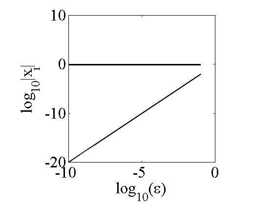
a)                                            b)

Figure 1: Newton polygon and roots of the polynomial $x^{3}+\epsilon x^{2}-x+\epsilon^{2}$. a) The Newton polygon edges are indicated by thick lines and the limiting monomials all satisfy the sign condition. The slopes of the edges are $0$ and $-2$ corresponding to leading terms in the Newton-Puiseux series of orders $\epsilon^{0}$ or $\epsilon^{2}$, respectively. b) The absolute values of the polynomial’s roots are represented vs. $\epsilon$, in logarithmic scale; the slopes are the roots valuations.

Fast variables of chemical reactions networks with multiple timescales satisfy quasi-stationarity equations. These are multivariate polynomial equations of the type

$$P(x_{1},x_{2},\ldots,x_{n},\epsilon)=\sum_{j}k_{j}\epsilon^{\gamma_{j}}x_{1}^{(\alpha_{j})_{1}}x_{2}^{(\alpha_{j})_{2}}\ldots x_{n}^{(\alpha_{j})_{n}}=0,$$ (3.6)

where $\gamma_{j}$ are integers and $(\alpha_{j})_{k}$ are positive integers. Let us note that $P(x)\in K[x_{1},x_{2},\ldots,x_{n}]$. Like in the case of the univariate equation (3.2), the tropical equilibrations provide lowest order approximations of the solutions of (3.6). We want to represent solutions of (3.6) by series, in other words we want to lift the tropical solutions to Newton-Puiseux series. In the univariate case, this is always possible by the Puiseux theorem. In the multivariate case, the lifting as Newton-Puiseux series of any tropical solution is ensured by a theorem of Kapranov [4]. In order to formulate this result let us introduce the valuation function $Val(x)$ defined as the lowest power of $\epsilon$ occurring in some Newton-Puiseux series $x(\epsilon)$. When applied to species concentrations $x_{i}$, kinetic parameters $k_{i}$ and monomials $k_{i}x^{\alpha_{i}}$ the valuation gives the orders $a_{i}$, $\gamma_{i}$ and $\mu_{i}$, respectively. As it can be easily checked

$$Val(x(\epsilon))=\lim_{\epsilon\to 0}\log_{\epsilon}|x(\epsilon)|$$

Suppose that the tropical equilibration condition defined in the introduction (Eq.(2.7)) is satisfied. By the same method as in the univariate case it can be shown that (2.7) is a necessary condition to have real Newton-Puiseux solutions. The Kapranov theorem [4] states that (2.7) is also a sufficient condition for having Newton-Puiseux solutions with prescribed lowest orders $(a_{1},a_{2},\ldots,a_{n})$. More precisely, there are $x_{i}(\epsilon)\in K$ such that $Val(x_{i})=a_{i}$ and such that $P(x_{1}(\epsilon),x_{2}(\epsilon),\ldots,x_{n}(\epsilon),\epsilon)=0$.

There is no analogue of Kapranov theorem working for systems of equations. In this case, the condition (2.7) though necessary, is not sufficient for guaranteeing the existence of Newton-Puiseux solutions.

In general, in order to obtain tropical equilibrations that can be lifted to Newton-Puiseux series we need to find a so-called tropical basis [1]. Let us consider that we want to find approximate solutions of $n$ equations of the form (3.6), namely

$$P_{1}(\mathbold{x},\epsilon)=0,\,P_{2}(\mathbold{x},\epsilon)=0,\,\ldots,P_{n}(\mathbold{x},\epsilon)=0$$ (3.7)

We first look for vectors $(a_{1},a_{2},\ldots,a_{n})\in{\mathbb{R}}^{n}$ satisfying the tropical equilibration condition (2.7) for each polynomial $P_{k}$, $k\in[1,n]$. This set is included in the tropical prevariety. Contrary to the case of one equation, it is not longer guaranteed that there are solutions $x_{1}(\epsilon),x_{2}(\epsilon),\ldots,x_{n}(\epsilon)$ of (3.7) such that

$$Val(x_{1},x_{2},\dots,x_{n})=(a_{1},a_{2},\dots,a_{n}),$$ (3.8)

where $Val$ means here application of the valuation componentwise. Solutions of (3.7) that satisfy (3.8) can be found if we solve a more complex problem. Let us supplement the system (3.7) with sums of products of the polynomials $P_{1},P_{2},\ldots,P_{n}$ by arbitrary polynomials and solve the tropical equilibration problem for the augmented system. In other words, let us look for solutions in the tropical variety of the ideal $I$ generated by $P_{1},P_{2},\ldots,P_{n}$. By a result of [27] in this case there are Newton-Puiseux solutions that satisfy the property (3.8). Although the ideal has an infinite number of elements, it can be shown that it is enough to solve the tropical problem for a finite set of polynomials in the ideal. A finite set of polynomials $f_{1},f_{2},\ldots,f_{t}$ generating the ideal $I$ and such that $T(f_{1})\cap T(f_{2})\cap\ldots\cap T(f_{t})=T(I)$ is called tropical basis. An algorithm for computing a tropical basis can be found in [1]. However, the complexity of this algorithm can be double-exponential in the size of the system, both in time and in space. In the remaining of this section we state a simple method for finding tropical solutions that can be lifted to Newton-Puiseux series.

Generically, a system of $n$ tropical equations in $n$ variables has a finite number of solutions. Indeed, the equality of two $n$-variate monomials corresponds to a $(n-1)$-dimensional hyperplane in the space of coordinates $\log(x_{i})$, or, equivalently, in the orders $a_{i}$. The intersection of $n$ hyperplanes of dimension $(n-1)$ in a $n$-dimensional space is generically a point. Because the combinations of monomials that can be equilibrated are finite, the total number of solutions is finite. However, chemical reactions systems often have infinite branches of tropical equilibrations. For instance, a reversible reaction can equilibrate both reactants and reaction products. In quasi-equilibrium conditions, the forward and reverse rate monomials of this reaction are dominant, have equal orders and occur in equilibration equations of several variables. Therefore, some of the hyperplanes resulting from different tropical equations coincide. In these cases, there are infinite sets of tropical equilibrations.

As an example, we can consider the following system of equations:

$$y-x-\epsilon x^{4}=0$$

$$x-y+\epsilon y^{2}=0$$ (3.9)

The valuations $a_{1}=Val(x(\epsilon))$ and $a_{2}=Val(y(\epsilon))$ of solutions of (3.9) satisfy the tropical equations $\min(a_{1},1+4a_{1})=\min(a_{1},1+2a_{2})=a_{2}$. The condition $\min(a_{1},1+4a_{1})=a_{1}$, leads to the infinite branch of solutions $a_{1}=a_{2}\geq-1/3$. The condition $\min(a_{1},1+4a_{1})=1+4a_{1}$ leads to $\min(a_{1},1+2a_{2})=\min(a_{1},3+8a_{1})=3+8a_{1}=1+4a_{1}$, therefore $a_{1}=-1/2$, $a_{2}=-1$, or to $\min(a_{1},3+8a_{1})=a_{1}=1+4a_{1}$, hence $a_{1}=a_{2}=-1/3$ solution already found. Thus the system (3.9) has an infinite branch of tropical equilbrations $a_{1}=a_{2}\geq-1/3$ and a isolated solution $a_{1}=-1/2$, $a_{2}=-1$.

However, only two of these solutions lead to Newton-Puiseux solutions of (3.9). Indeed, the system (3.9) has $7$ complex solutions, namely $(0,0)$, $(x,\pm x^{2})$, where $x$ is a solution of $\epsilon x^{3}\mp x+1=0$. Using the Newton polygon construction we find that the possible valuations of $x$ are $0$ or $-1/2$. It follows that valuations of real Newton-Puiseux solutions of Eq. (3.9) are $(0,0)$, or $(-1/2,-1)$. The only tropical solutions leading to Newton-Puiseux series is $(0,0)$, a point on the continuous, infinite branch of tropical solutions and $(-1/2,-1)$, the isolated solution.

We conjecture that all the isolated tropical equilibrations can be extended to Newton-Puiseux series. Therefore, if by supplementing the original system with sums or products of the original equations with arbitrary polynomials (i.e. considering the ideal generated by these equations) we find a system with only isolated tropical equilibrations, we believe that all of them can be lifted to Newton-Puiseux series. For instance, in the above example, let us consider together to the equations (3.9) also their sum $\epsilon(y^{2}-x^{4})=0$ and solve the resulting extended tropical system $\min(a_{1},1+4a_{1})=\min(a_{1},1+2a_{2})=a_{2},\quad a_{1}=a_{2}/2$. This system has only two solutions, $(0,0)$ and $(-1/2,-1)$. These two solutions are isolated. We have already shown that they can be lifted to Newton-Puiseux series. An ansatz for finding linear combinations of equations leading to isolated tropical equilibrations is to consider conservations laws of the fast subsystem. This ansatz will be used in the Sections 4,5.

4 Model reduction of biochemical reaction newtworks with fast cycles.

In this section we introduce our model reduction method. We also state and prove our main result on the existence of invariant manifolds for networks with fast species and fast cycles.

Let us call tropically truncated system associated to the tropical equilibration $(a_{1},a_{2},\ldots,a_{n})$, the system obtained by pruning all the dominated monomials of (2.1) revealed by the rescaling (2.4), i.e.

$$\frac{\mathrm{d}x_{i}}{\mathrm{d}t}=\sum_{j\in J(i)}k_{j}S_{ij}{{\mathbold{x}}}^{\mathbold{\alpha_{j}}},\quad i\in[1,n]$$ (4.1)

where $J(i)=\underset{j}{\operatorname*{\arg\!\min}}(\mu_{j},S_{ij}\neq 0)$ is the set of dominating reaction rates of reactions acting on species $i$ and $\mu_{j}$ are defined by (2.5).

Like in the introduction, we introduce the orders $\nu_{i}=\mu_{J(i)}-a_{i}$, with $\mu_{J(i)}=\min(\mu_{j},S_{ij}\neq 0)$. The rescaled truncated system reads

$$\frac{\mathrm{d}\bar{x}_{i}}{\mathrm{d}t}=\varepsilon^{\nu_{i}}\sum_{j\in J(i)}\bar{k}_{j}S_{ij}{\bar{\mathbold{x}}}^{\mathbold{\alpha_{j}}},\quad i\in[1,n].$$ (4.2)

Variables $x_{i}$ with smaller orders $\nu_{i}$ are faster. After reordering the variables we can consider that $\nu_{1}\leq\nu_{2}\leq\ldots\leq\nu_{n}$. Let us assume that the following gap condition is fulfilled:

$$\text{there is }f<n\text{ such that }\nu_{f+1}-\nu_{f}>0,$$ (4.3)

meaning that two groups of variables have separated timescales. The variables $\mathbold{x}_{f}=(x_{1},x_{2},\ldots,x_{f})$ are fast (change significantly on timescales of order of magnitude $\epsilon^{-\nu_{f}}$ or shorter). The remaining variables $\mathbold{x}_{s}=(x_{f+1},x_{f+2},\ldots,x_{n})$ are slow (have little variation on timescales of order of magnitude $\epsilon^{-\nu_{f}}$).

We call linear conservation law of a system of differential equations, a linear form $c(\mathbold{x})=<\mathbold{c},\mathbold{x}>=c_{1}x_{1}+c_{2}x_{2}+\ldots+c_{n}x_{n}$ that is identically constant on trajectories of the system. It can be easily checked that vectors in the left kernel $Ker^{l}(S)$ of the stoichiometric matrix $\mathbold{S}$ provide linear conservation laws of the system (2.1). Indeed, system (2.1) reads $\frac{\mathrm{d}\mathbold{x}}{\mathrm{d}t}=\mathbold{S}\mathbold{R}(\mathbold{x})$, where the components of the vector $\mathbold{R}$ are $R_{j}(\mathbold{x})=k_{j}x^{\alpha_{j}}$. If $\mathbold{c}^{T}\mathbold{S}=0$, then $\frac{\mathrm{d}<\mathbold{c},\mathbold{x}>}{\mathrm{d}t}=\mathbold{c}^{T}\mathbold{S}\mathbold{R}(\mathbold{x})=0$, where $\mathbold{c}^{T}=(c_{1},c_{2},\ldots,c_{n})$.

Let us assume that the truncated system (4.1), restricted to the fast variables has a number of independent, linear conservation laws, defined by the vectors $\mathbold{c}_{1},\mathbold{c}_{2},\ldots,\mathbold{c}_{r}$, where $\mathbold{c}_{k}=(c_{k1},c_{k2},\ldots,c_{kn})$. These conservation laws can be calculated by recasting the truncated system as the product of a new stoichiometric matrix and a vector of monomial rate functions and further computing left kernel vectors of the new stoichiometric matrix. We further assume that the truncated system and the full system (4.1) have no conservation laws in common.

We now define the new variables $y_{k}=\sum_{l}c_{kl}x_{l}$, where $k\in[1,r]$. These new variables satisfy the equations

$$\frac{\mathrm{d}y_{k}}{\mathrm{d}t}=\sum_{j}\sum_{l}c_{kl}S_{lj}\mathbold{x}^{\mathbold{\alpha_{j}}}.$$ (4.4)

Let $(a_{1},a_{2},\ldots,a_{n})$ be a solution of the tropical equilibration problem for the augmented system obtained by putting together (2.1) and (4.4). We define $b_{k}=\min(a_{l},c_{kl}\neq 0)$ and $\rho_{k}=\mu_{J_{c}(k)}-b_{k}$ where $\mu_{J_{c}(k)}=\min(\mu_{j},c_{kl}\neq 0,S_{lj}\neq 0)$, $J_{c}(k)=\underset{j}{\operatorname*{\arg\!\min}}(\mu_{j},c_{kl}\neq 0,S_{lj}\neq 0)$. In rescaled variables $y_{k}=\bar{y}_{k}\epsilon^{b_{k}}$ we have the following truncated rescaled system

$$\frac{\mathrm{d}\bar{y}_{k}}{\mathrm{d}t}=\epsilon^{\rho_{k}}\sum_{j\in J_{c}(k)}\sum_{l}c_{kl}S_{lj}\bar{\mathbold{x}}^{\mathbold{\alpha_{j}}}.$$ (4.5)

We assume that $\nu_{f}<\rho_{k}$, meaning that the variables $y_{k},k\in[1,r]$ are slower than the variables $x_{i},i\in[1,r]$.

Since we have $r$ conservation laws, we can eliminate $r$ fast variables from the truncated system. One can suppose that these fast variables are $x_{f-r+1},...,x_{f}$ can be expressed via the remaining variables $x_{i}$, $i\in[1,f-r]$ and $y_{k}$, $k\in[1,r]$. Let us introduce vectors

$$\mathbold{X}_{r}=(\bar{x}_{1},\bar{x}_{2},\ldots,\bar{x}_{f-r}),\quad\mathbold{X}_{s}=(\bar{x}_{f+1},\bar{x}_{f+2},\ldots,\bar{x}_{n}),\quad\bar{\mathbold{y}}=(\bar{y}_{1},\bar{y}_{2},\ldots,\bar{y}_{r}).$$

Then any function of $\bar{\mathbold{x}}$ can be expressed via $\mathbold{X}_{r},\mathbold{X}_{s}$ and $\bar{\mathbold{y}}$. As a result, we obtain the following decomposition

$$\frac{\mathrm{d}\bar{x}_{i}}{\mathrm{d}t}=\varepsilon^{\nu_{i}}F_{i}(\mathbold{X}_{r},\bar{\mathbold{y}},\mathbold{X}_{s},\epsilon)\ \quad i\in[1,f-r],$$ (4.6)

where

$$F_{i}(\mathbold{X}_{r},\bar{\mathbold{y}},\mathbold{X}_{s},\epsilon)=\sum_{j\in J(i)}\bar{k}_{j}S_{ij}{\bar{\mathbold{x}}}^{\mathbold{\alpha_{j}}},$$

$$\frac{\mathrm{d}\bar{x}_{i}}{\mathrm{d}t}=\varepsilon^{\nu_{i}}S_{i}(\mathbold{X}_{r},\bar{\mathbold{y}},\mathbold{X}_{s},\epsilon),\quad i\in[f+1,n],$$ (4.7)

$$S_{i}(\mathbold{X}_{r},\bar{\mathbold{y}},\mathbold{X}_{s},\epsilon)=\sum_{j\in J(i)}\bar{k}_{j}S_{ij}{\bar{\mathbold{x}}}^{\mathbold{\alpha_{j}}},$$

$$\frac{\mathrm{d}\bar{y}_{k}}{\mathrm{d}t}=\epsilon^{\rho_{k}}Y_{k}(\mathbold{X}_{r},\bar{\mathbold{y}},\mathbold{X}_{s},\epsilon),\quad k\in[1,r],$$ (4.8)

$$Y_{k}(\mathbold{X}_{r},\bar{\mathbold{y}},\mathbold{X}_{s},\epsilon)=\sum_{j\in J_{c}(k)}\sum_{l}c_{kl}S_{lj}\bar{\mathbold{x}}^{\mathbold{\alpha_{j}}},$$

where $\mathbold{Y}$, $\mathbold{S}$ and $\mathbold{F}$ are analytic functions.

The system (4.6) describes the evolution of fast modes. Because it was obtained from the truncated versions of the first $f-r$ equations of (2.1), let us call it the fast truncated subsystem. As a matter of fact, the system (4.6) coincides with the first $f-r$ equations of (4.2).

Let us recall some notions of the dynamical systems theory. Let $d\mathbold{x}/dt=\mathbold{F}(\mathbold{x})$ be a system of ordinary differential equations defined on an open domain $\Omega$ of an Euclidean space with smooth boundary. Here $\mathbold{F}$ is a smooth function, for example, $\mathbold{F}\in C^{r}$, where $r>1$. Let us consider an equilibrium (steady state) $\mathbold{\phi}$ (i.e., the relation $\mathbold{F}(\mathbold{\phi})=0$ holds) of this system. Let $A$ be a linear operator that gives a linearization of r.h.s. of this system at $\mathbold{\phi}$:

$$\mathbold{F}(\mathbold{x})=A(\mathbold{x}-\mathbold{\phi})+O((\mathbold{x}-\mathbold{\phi})^{2}).$$

We say that this equilibrium is hyperbolic [22], if the distance $d$ between the spectrum $Spec_{A}$ of $A$ and the imaginary axis $I=\{z\in{\mathbb{C}}:Re\ z=0\}$ is not zero:

$$d=dist(SpecA,\ I)\neq 0.$$ (4.9)

If the spectrum lies in the left-half plane $\{z\in{\mathbb{C}}:Re\ z<0\}$, then this equilibrium is stable and locally attracting. In our case all systems depend on the parameter $\epsilon>0$, therefore, $d$ in (4.9) can depend on $\epsilon$.

We can now formulate our main result.

Theorem 4.1

Assume the gap condition (4.3) holds and that $\nu_{f}<\rho_{k}$, $k\in[1,r]$. Assume that for all values $\bar{\mathbold{y}}$ and $\mathbold{X_{s}}$ the fast truncated system (4.6) has a stable hyperbolic steady state

$$\bar{x}_{i}=\phi_{i}(\bar{\mathbold{y}},\mathbold{X_{s}})+\text{higher order terms},\quad i\in[1,f-r],$$

such that the distance $d(\epsilon)$ admits the estimate

$$d>C_{0}\epsilon^{\kappa}$$

where $\kappa\geq 0$ is small enough and $C_{0}$ is independent on $\epsilon$. Then for sufficiently small $\epsilon>0$ system (4.1) has a locally attracting and locally invariant normally hyperbolic $C^{p}$ ($p>1$) smooth manifold defined by

$$\bar{x}_{i}=\phi_{i}(\bar{\mathbold{y}},\mathbold{X_{s}},\epsilon)+\text{higher order terms},\quad i\in[1,f-r],$$ (4.10)

and the dynamics of the slow variables $\bar{\mathbold{y}},\bar{x}_{f+1},\bar{x}_{f+2},\ldots,\bar{x}_{n}$ for large times takes the form

$$\frac{\mathrm{d}\bar{x}_{i}}{\mathrm{d}t}=\epsilon^{\nu_{i}}\sum_{j\in J(f+1)}k_{j}S_{ij}{{\bar{\mathbold{x}}}_{s}}^{\mathbold{\alpha_{j}}}+\text{higher order terms},\quad i\in[f+1,n]$$

$$\frac{\mathrm{d}\bar{y}_{k}}{\mathrm{d}t}=\epsilon^{\rho_{k}}\sum_{j\in J_{c}(k)}\sum_{l}c_{kl}S_{lj}\bar{\mathbold{x}}_{s}^{\mathbold{\alpha_{j}}}+\text{higher order terms},\quad k\in[1,r]$$ (4.11)

where $\bar{\mathbold{x}}_{s}^{\mathbold{\alpha_{j}}}=\phi_{1}^{\alpha_{1}^{j}}\phi_{2}^{\alpha_{2}^{j}}\ldots\phi_{f}^{\alpha_{f}^{j}}\bar{x}_{f+1}^{\alpha_{f+1}^{j}}\bar{x}_{f+2}^{\alpha_{f+2}^{j}}\ldots\bar{x}_{n}^{\alpha_{n}^{j}}$.

Remark: “higher order terms” means some smooth functions of $\bar{\mathbold{y}},\mathbold{X_{s}},\epsilon$ having higher orders in $\epsilon$ with respect to principal terms.

Proof. We use the standard result, which follows from the theory of normally hyperbolic invariant manifolds [11]. Consider the system of differential equations

$$d\mathbold{u}/d\tau=Au+\lambda\mathbold{F}(\mathbold{u},\mathbold{v},\lambda)+\mathbold{H}(\mathbold{u},\mathbold{v},\lambda),$$ (4.12)

$$d\mathbold{v}/d\tau=\lambda^{\mu}\mathbold{S}(\mathbold{u},\mathbold{v},\lambda),\quad\mu>0,$$ (4.13)

where $u\in{\mathbb{R}}^{n}$, $v\in{\mathbb{R}}^{m}$, $A$ is a linear operator such that the spectrum of $A$ satisfies (4.9) and lies in the left-half plane, $F,G$ and $H$ are smooth functions uniformly bounded in $C^{k}$-norm on ${\mathbb{R}}^{n}\times{\mathbb{R}}^{m}\times[0,1]$ for some $k>1$. Moreover, $H=O(|\mathbold{u}|^{2})$ as $\mathbold{u}\to 0$.

It is clear that this system becomes slow/fast for small $\lambda>0$, where $u$ are fast and $v$ are slow. For any $p<k$ and sufficiently small $\lambda$ there exists a normally hyperbolic smooth locally attracting invariant manifold close to $0$: $u=\lambda U(v,\lambda)$, where $U$ is bounded in $C^{p}$ -norm.

To apply this result, we reduce our system (2.1) to the form (4.12), (4.13). We introduce $u=\mathbold{X_{r}}-\mathbold{\phi}$ and makes a time change $\tau=\epsilon^{\kappa}t$. We introduce the variables $v$ by $v=(\mathbold{X}_{s},\bar{\mathbold{y}})$. Then, if $\kappa>0$ is small enough we obtain that system (4.6), (4.7), (4.8) can be rewritten in the form (4.12), (4.13) with $\lambda=\epsilon^{\rho}$ for some $\rho>0$. This completes the proof. $\blacksquare$

5 A simple nonlinear cycle example.

Let us consider the following example of a cycle of reactions that includes a complex formation reaction:

$$A_{1}\overset{k_{1}}{\longrightarrow}A_{2}\overset{k_{2}}{\longrightarrow}A_{3}\overset{k_{3}}{\longrightarrow}A_{1},\quad A_{1}+A_{2}\underset{k_{5}}{\overset{k_{4}}{\rightleftharpoons}}A_{3}$$

The mass action chemical kinetic equations for this cycle read:

$$\frac{\mathrm{d}x_{1}}{\mathrm{d}t} = -k_{1}x_{1}+k_{3}x_{3}-k_{4}x_{1}x_{2}+k_{5}x_{3}$$ (5.1)

$$\frac{\mathrm{d}x_{2}}{\mathrm{d}t} = k_{1}x_{1}-k_{2}x_{2}-k_{4}x_{1}x_{2}+k_{5}x_{3}$$ (5.2)

$$\frac{\mathrm{d}x_{3}}{\mathrm{d}t} = -k_{3}x_{3}+k_{2}x_{2}+k_{4}x_{1}x_{2}-k_{5}x_{3}$$ (5.3)

Consider kinetic constants that scale like $k_{i}\sim\epsilon^{\gamma_{i}}$. For instance if $\epsilon=1/10$ and $k_{1}=1,k_{2}=0.1,k_{3}=0.01,k_{4}=0.01,k_{5}=0.001$ we get

$$\gamma_{1}=0,\gamma_{2}=1,\gamma_{3}=\gamma_{4}=2,\gamma_{5}=3.$$ (5.4)

The tropical equilibrations for this model are the solutions of the following min-plus equations

$$\min(\gamma_{1}+a_{1},\gamma_{4}+a_{1}+a_{2})=\min(\gamma_{3},\gamma_{5})+a_{3}=\min(\gamma_{2}+a_{2},\gamma_{4}+a_{1}+a_{2})=\min(\gamma_{1}+a_{1},\gamma_{5}+a_{3}),$$ (5.5)

where the first, second and third equality of (5.5) follow from (5.1), (5.2), (5.3), respectively. Because $\gamma_{3}<\gamma_{5}$ we have $\min(\gamma_{3},\gamma_{5})=\gamma_{3}$. From (5.5) it follows that $\gamma_{3}+a_{3}=\min(\gamma_{1}+a_{1},\gamma_{5}+a_{3})$. Furthermore $\min(\gamma_{1}+a_{1},\gamma_{5}+a_{3})=\gamma_{1}+a_{1}$ (because $\gamma_{5}+a_{3}>\gamma_{3}+a_{3}$). Hence, in this case, the system of min-plus equations can be simplified to

$$\min(\gamma_{1}+a_{1},\gamma_{4}+a_{1}+a_{2})=\gamma_{3}+a_{3}=\min(\gamma_{2}+a_{2},\gamma_{4}+a_{1}+a_{2})=\gamma_{1}+a_{1}$$ (5.6)

Only one of the possible outputs of the first $\min$ operation (5.6) has to be considered, namely $\min(\gamma_{1}+a_{1},\gamma_{4}+a_{1}+a_{2})=\gamma_{1}+a_{1}$, whereas the second $\min$ leads to two situations. It follows that there are thus two branches of tropical solutions, namely:

$$a_{1}\geq\gamma_{2}-\gamma_{4},\quad a_{2} =a_{1}+\gamma_{1}-\gamma_{2},\quad a_{3}=a_{1}+\gamma_{1}-\gamma_{3}$$ (5.7)

$$a_{1}\leq\gamma_{2}-\gamma_{4},\quad a_{2} =\gamma_{1}-\gamma_{4},\quad a_{3}=a_{1}+\gamma_{1}-\gamma_{3}$$ (5.8)

The tropical equilibration solutions vary continuously on each of the branch and are non-isolated. It is thus possible that some tropical solutions or an entire branch can not be lifted to Newton-Puiseux series. In order to find solutions that can be lifted we will consider equations in the ideal of (5.1), (5.2), (5.3), starting with the conservation laws of the fast subsystem. It will come out that this is enough, as adding these conservation laws leads to isolated tropical equilibrations.

Let us first consider the branch (5.7). By keeping dominating monomials of lowest order in $\epsilon$ and pruning all the others we get the following truncated system:

$$(T)\left\{\begin{array}[]{lll}\frac{\mathrm{d}\bar{x}_{1}}{\mathrm{d}t}&=&\epsilon^{\gamma_{1}}(-\bar{k}_{1}\bar{x}_{1}+\bar{k}_{3}\bar{x}_{3})\\ \frac{\mathrm{d}\bar{x}_{2}}{\mathrm{d}t}&=&\epsilon^{\gamma_{2}}(\bar{k}_{1}\bar{x}_{1}-\bar{k}_{2}\bar{x}_{2})\\ \frac{\mathrm{d}\bar{x}_{3}}{\mathrm{d}t}&=&\epsilon^{\gamma_{3}}(-\bar{k}_{3}\bar{x}_{3}+\bar{k}_{2}\bar{x}_{2}),\end{array}\right.$$ (5.9)

The truncated system (5.9) have the linear first integral (conservation law)

$$y=x_{1}+x_{2}+x_{3}.$$ (5.10)

The variable $y$ is not a first integral of the full system, which implies that the truncated system $(T)$ can not be a good approximation at large times. The exact dynamics of $y$ is obtained by summing the equations (5.1),(5.2),(5.3):

$$\frac{\mathrm{d}y}{\mathrm{d}t}=-k_{4}x_{1}x_{2}+k_{5}x_{3}.$$ (5.11)

We consider that $y\sim\epsilon^{a_{y}}$ and further equilibrate the equations (5.10),(5.11). We therefore get two more min-plus equations:

$$a_{y}=\min(a_{1},a_{2},a_{3})$$ (5.12)

$$\gamma_{4}+a_{1}+a_{2}=\gamma_{5}+a_{3}$$ (5.13)

Assume the particular choice (5.4) of parameter orders. Then, for the tropical solution (5.7), it follows $a_{1}=0$, $a_{2}=-1$, $a_{y}=a_{3}=-2$, $\nu_{1}=0$, $\nu_{2}=1$, $\nu_{3}=2$, $\nu_{y}=3$ which means that $y$ is slower than $x_{i},1\leq i\leq 3$. The resulting tropical equilibration is in fact unique and thus isolated. Indeed, considering the second branch of tropical equilibrations for the variables $x_{1},x_{2},x_{3}$ (5.8) we find that $y$ can not be equilibrated because (5.13) and (5.8) imply $\gamma_{5}=\gamma_{3}$ which is not satisfied. The polynomial defining the dynamics of $y$ being in the ideal of polynomials defining the dynamics of $x_{1},x_{2},x_{3}$, it follows that the branch (5.8) is not in the tropical variety and can be discarded.

We will now use this isolated tropical equilibration to obtain reduced models. We will discuss three reduced models: the truncated model $(T)$ in (5.9) that describes the relaxation dynamics towards the attractive invariant manifold, the reduced model (4.11) given by Theorem 4.1 and describing dynamics on the invariant manifold, and a third reduced model combining these two.

The truncated system (5.9) copes only with the fast relaxation onto the invariant manifold. The tropical approximation of the invariant manifold is obtained by setting the l.h.s of (5.9) to zero, i.e. computing the steady states of the truncated system. This approximation is the half-line $x_{2}=k_{1}k_{2}^{-1}x_{1},x_{3}=k_{1}k_{3}^{-1}x_{1},x_{1}<k_{2}k_{4}^{-1}$. By using the new tropically truncated equation:

$$y=x_{3},$$ (5.14)

we compute $x_{1}$, $x_{2}$, $x_{3}$ from $y$ and obtain the reduced model:

$$(R)\left\{\begin{array}[]{ll}\frac{\mathrm{d}y}{\mathrm{d}t}&=-k_{1}^{-1}k_{2}^{-1}k_{3}^{2}k_{4}y^{2}+k_{5}y\\ x_{1}&=k_{1}^{-1}k_{3}y,\,x_{2}=k_{2}^{-1}k_{3}y,\,x_{3}=y\end{array}\right.$$ (5.17)

The reduced model $(R)$ (5.17) copes with the slow dynamics on the invariant manifold.

In this particular example the two approximations $(T)$ and $(R)$ are composable, i.e. they can be merged in a model with broader validity. By replacing $y$ with $x_{3}$ in (5.17) and combining the resulting equations with the truncated system $(T)$ we get the following model:

$$(M)\left\{\begin{array}[]{lll}\frac{\mathrm{d}x_{1}}{\mathrm{d}t}&=&-k_{1}x_{1}+k_{3}x_{3}\\ \frac{\mathrm{d}x_{2}}{\mathrm{d}t}&=&k_{1}x_{1}-k_{2}x_{2}\\ \frac{\mathrm{d}x_{3}}{\mathrm{d}t}&=&-k_{3}x_{3}+k_{2}x_{2}-k_{1}^{-1}k_{2}^{-1}k_{3}^{2}k_{4}x_{3}^{2}+k_{5}x_{3}\end{array}\right.$$ (5.21)

The model $(M)$ is a multiscale reduction as it gives accurate approximations of both fast and slow parts of the trajectories.

The comparison of different approximations is shown in Figure 2. The validity of the multiscale reduction could depend on the initial data. We have determined numerically the domain of initial data leading to accurate reductions. Starting from the same initial data we have integrated the full model (5.1),(5.2),(5.3) and the reduced model (5.21) and obtained the trajectories $x(t)$ and $xr(t)$, respectively. We have computed the error such as Hausdorff-Pompeiu distance between the sets $\{(log_{10}(t),log_{10}(x_{1}(t)),log_{10}(x_{2}(t)),log_{10}(x_{3}(t))),\text{variable}\,t\}$ and $\{(log_{10}(t),log_{10}(xr_{1}(t)),log_{10}(xr_{2}(t)),log_{10}(xr_{3}(t))),\text{variable}\,t\}$. We notice in Figure 3a) that we can change the initial data on $7$ decades and still keep the trajectories of the reduced model (5.21) close to the trajectories of the full model (5.1),(5.2),(5.3).

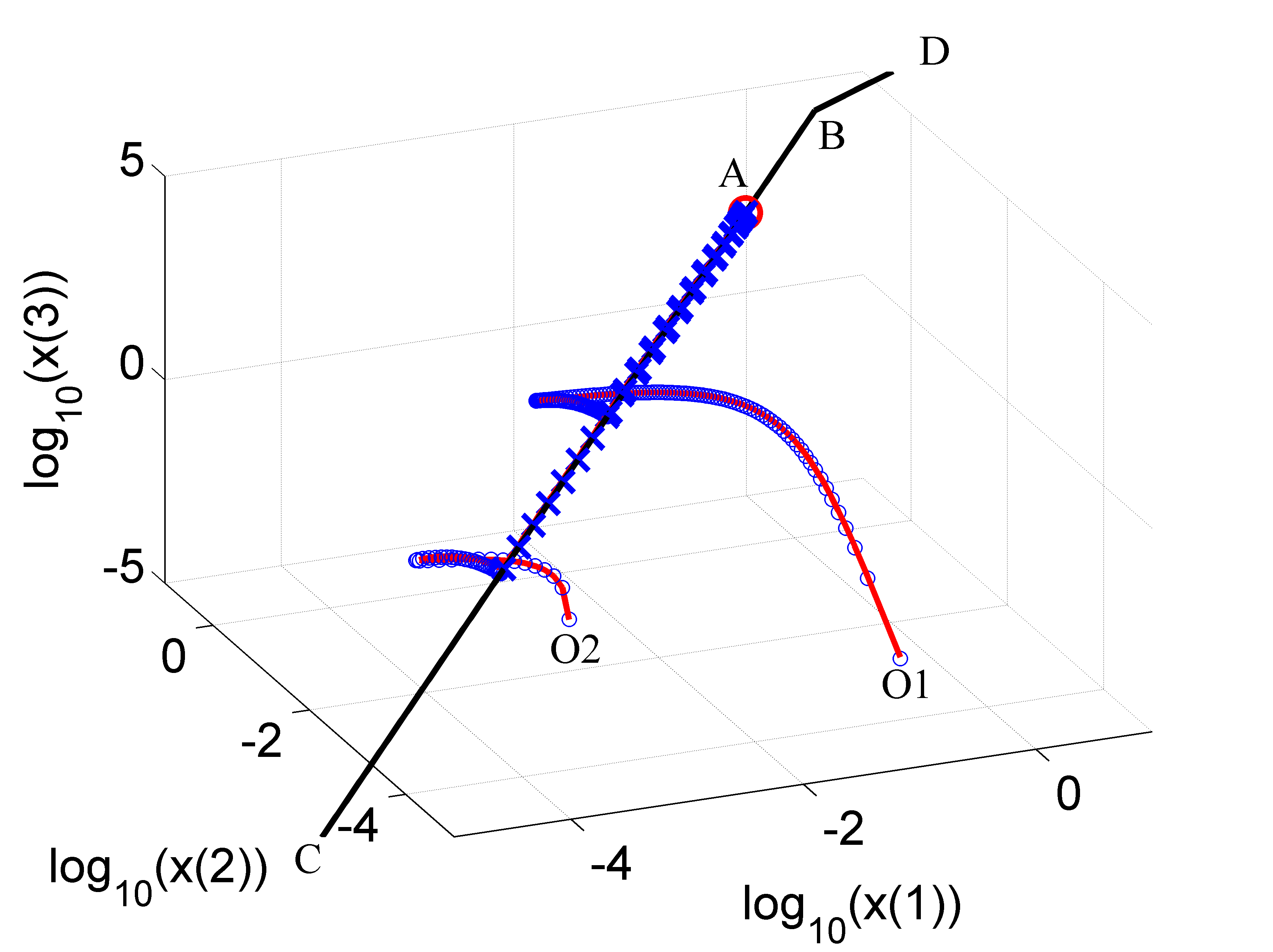
Figure 2: Two trajectories of the nonlinear cycle model defined by Eqs.(5.1),(5.2),(5.3) starting from $O_{1}$ and $O_{2}$ are represented in red solid line. The blue circles are the trajectories starting from $O_{1}$ and $O_{2}$ computed with the tropical truncated model $(T)$ defined by Eqs.(5.9). The blue crosses are the trajectories computed with the reduced model defined by Eqs.(5.17). $A$ is the stable steady state of the model. The half-lines $BC$ and $BD$ belong to parts of tropical variety corresponding to the tropical solutions $a_{1}\geq-1,\quad a_{2}=a_{1}-1,\quad a_{3}=a_{1}-2$ and $a_{1}\leq-1,\quad a_{2}=-2,\quad a_{3}=a_{1}-2$, respectivelly.

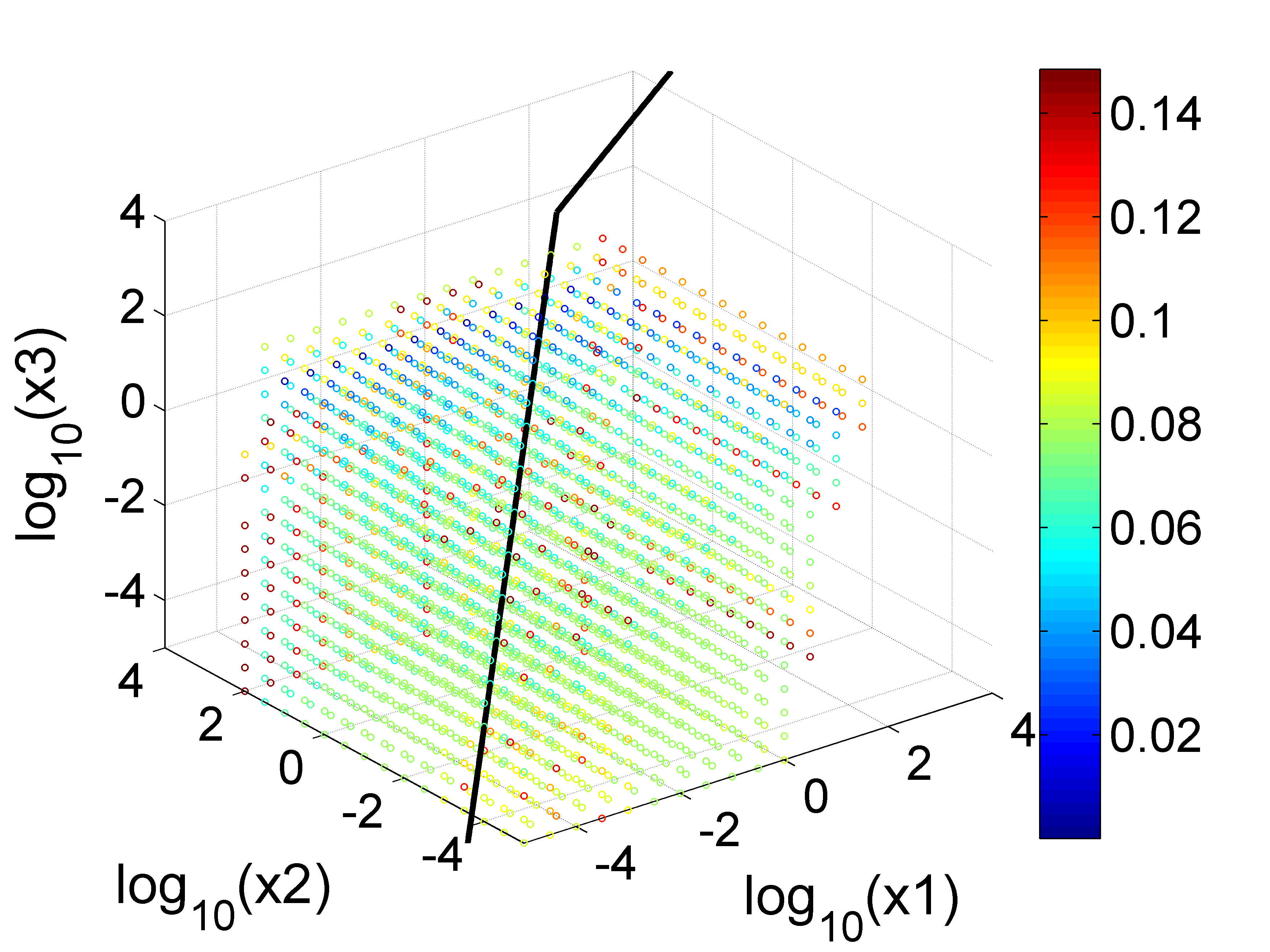
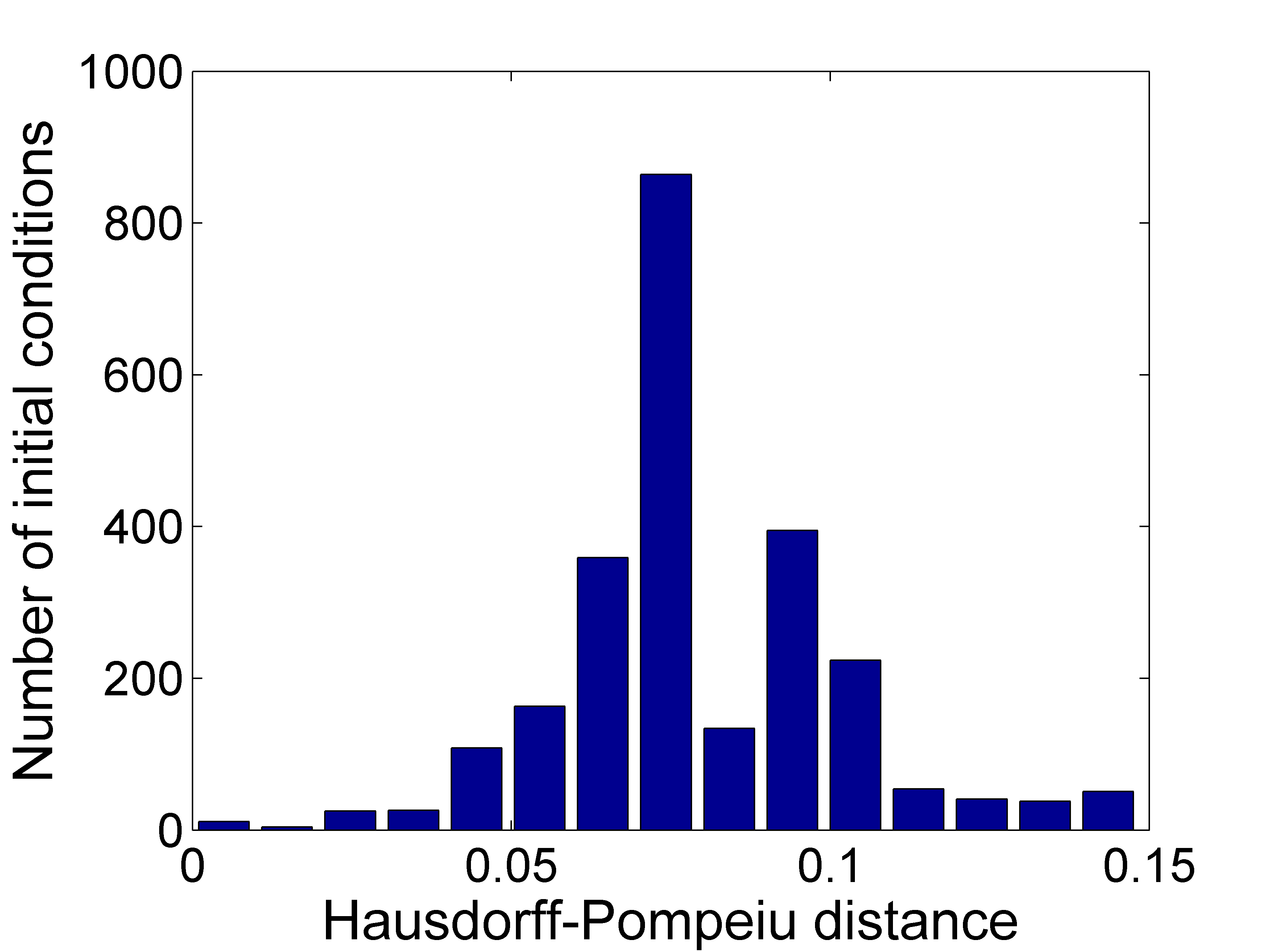
a)                                            b)

Figure 3: Trajectories of full (Eqs.(5.1),(5.2),(5.3)) and multiscale reduced model (Eqs.(5.21)) were computed starting from the same initial conditions and the Hausdorff-Pompeiu distance between the corresponding sets $\{(log_{10}(t),log_{10}(x_{1}),log_{10}(x_{2}),log_{10}(x_{3})),\text{variable}\,t\}$ were calculated. The initial conditions where chosen from an uniform grid in logarithmic scale $-5\leq log_{10}(x_{1})\leq 4$, $-5\leq log_{10}(x_{2})\leq 2$, $-5\leq log_{10}(x_{3})\leq 4$. a) The positions of the initial data leading to Hausdorff-Pompeiu distance less than $0.15$ are shown by circles with color coded values of this distance. The lines indicates the same parts of tropical variety as in Fig.2. Initial data can vary on $7$ decades with global relative errors less than $1-10^{0.15}\approx 0.4$ which for $\epsilon=1/10$ and stiff trajectories is remarkably robust. b) The distribution of Hausdorff-Pompeiu distances is shown for the set of initial data.

6 Conclusion

We have shown how to relate the tropical equilibration problem to the slow-fast decomposition and model reduction of biochemical reactions networks. In the case of biochemical networks with mass action kinetics, we use tropical equilibration solutions to find which species are fast and which are slow. We have proposed elsewhere two methods for solving the tropical equilibration problem, a first one by reformulating it as a constraint satisfaction problem [26] and a second one based on the Newton polyhedron [23].

Under rather general conditions, existence of small dimensional attractive invariant manifolds for reactions networks with fast cycles and species is shown.

Our model reduction recipe consists in calculating tropical equilibration solutions at least twice. At the first step we solve the tropical equilibration problem for the initial system of differential equations. This allows us to identify the fast species, that constitute the fast subsystem of the model. The fast truncated system, obtained by pruning dominated monomials in the equations of fast species, copes with relaxation towards the attracting invariant manifold. The tropical equilibrations calculated at this step belong to the tropical prevariety, but not all of them lead to a reduced model. In order to filter tropical solutions we solve the tropical equilibration problem a second time. If the fast truncated subsystem has conservation laws different from the ones of the full system, we use them to define new slow variables. At the second step, we solve the tropical equilibration problem for the augmented system that is obtained by adding to the initial system the differential equations satisfied by the conservation laws of the fast truncated subsystem. These new equations are linear combinations of the initial ones. We conjecture that if the resulting solutions are isolated, then they belong to the tropical variety. Also, they lead to reduced models obtained by expressing fast variables in terms of the slow variables. The resulting reduced model copes with the dynamics on the invariant manifold. If after the second step one still has truncated systems with conservation laws and continuous branches of tropical equilibrations, the first two steps can be reiterated until there are no conservation laws different from the ones of the full model and all tropical equilibrations are isolated.

Our method can be used as recipe for formal model reduction in computational biology. Some steps of the recipe are already automated, such as the calculation of tropical equilibrations. The computation of conservation laws can be performed by methods from [25], but we don’t exclude the existence of difficult cases when conservation laws are not enough for grasping the tropical variety. In these difficult cases, calculation of tropical basis can use methods from [1]. Another challenging step is the elimination of fast variables as solutions of systems of polynomial equations. When the polynomials of the fast truncated system contain only two monomials, we can apply rapid methods for toric systems [16, 10]. In general, fast truncated systems are fewnomials (have a small number of monomials) and can be approached by the methods for sparse polynomial systems [10]. However, even with fewnomials, there could be models for which the elimination of fast variables is difficult. Numerical methods can be used, as a last resort, to solve problematic cases.

For a simple example, we suggested, without providing a general recipe, how to combine one-scale approximations to obtain a multiscale approximation that is valid on both fast and slow time scales. A general method for obtaining multiscale approximations was given in [8] for networks of monomolecular reactions (in these networks each reaction has at most one reactant and at most one product and the reaction rates are given by the mass action law) with separated kinetic constants. Multiscale approximations of nonlinear networks are much more difficult and will be discussed elsewhere.

References

- [1] T. Bogart, A.N. Jensen, D. Speyer, B. Sturmfels, R.R. Thomas. Computing tropical varieties. Journal of Symbolic Computation, 42 (1) (2007), 54–73.
- [2] B.L. Clarke. General method for simplifying chemical networks while preserving overall stoichiometry in reduced mechanisms. J. Phys. Chem., 97 (1992), 4066–4071.
- [3] E.M. Clarke, R. Enders, T. Filkorn, S. Jha. Exploiting symmetry in temporal logic model checking. Formal Methods in System Design, 9 (1-2) (1996), 77–104.
- [4] M. Einsiedler, M. Kapranov, D. Lind. Non-archimedean amoebas and tropical varieties. Journal für die reine und angewandte Mathematik (Crelles Journal), (601) (2006), 139–157.
- [5] D. Eisenbud. Commutative Algebra with a View Toward Algebraic Geometry. Springer-Verlag, 1995.
- [6] J. Feret, V. Danos, J. Krivine, R. Harmer, W. Fontana. Internal coarse-graining of molecular systems. Proceedings of the National Academy of Sciences, 106 (16) (2009), 6453–6458.
- [7] A.N. Gorban, I.V. Karlin. Invariant manifolds for physical and chemical kinetics, Lect. Notes Phys. 660. Springer, Berlin Heidelberg, 2005.
- [8] A.N. Gorban, O. Radulescu. Dynamic and static limitation in reaction networks, revisited. In: D.W. Guy, B. Marin, G.S. Yablonsky, editors. Advances in Chemical Engineering – Mathematics in Chemical Kinetics and Engineering. vol. 34 of Advances in Chemical Engineering. Elsevier, 2008, 103–173.
- [9] A.N. Gorban, O. Radulescu, A. Zinovyev. Asymptotology of chemical reaction networks. Chemical Engineering Science, 65 (7) (2010), 2310–2324.
- [10] D. Grigoriev, A. Weber. Complexity of solving systems with few independent monomials and applications to mass-action kinetics. In: V. P. Gerdt, W. Koepf, E.W. Mayr, E.V. Vorozhtsov, editors. Computer Algebra in Scientific Computing, vol. 7442 of Lecture Notes in Computer Science. Springer, Berlin Heidelberg, 2012, 143–154.
- [11] A. Katok, B. Hasselblatt. Introduction to the Modern Theory of Dynamical Systems. Cambridge University Press, 1996.
- [12] E.L. King, C.A. Altman. A schematic method of deriving the rate laws for enzyme-catalyzed reactions. J. Phys. Chem., 60 (1956), 1375–1378.
- [13] S.H. Lam, D.A. Goussis. The CSP method for simplifying kinetics. International Journal of Chemical Kinetics, 26 (4) (1994), 461–486.
- [14] U. Maas, S.B. Pope. Simplifying chemical kinetics: intrinsic low-dimensional manifolds in composition space. Combustion and Flame, 88 (3) (1992), 239–264.
- [15] D. Maclagan, B. Sturmfels. Introduction to tropical geometry. Graduate Studies in Mathematics, vol. 161, 2009.
- [16] M.P. Millán, A. Dickenstein, A. Shiu, C. Conradi. Chemical reaction systems with toric steady states. Bulletin of mathematical biology, 74 (5) (2012), 1027–1065.
- [17] V. Noel, D. Grigoriev, S. Vakulenko, O. Radulescu. Tropical geometries and dynamics of biochemical networks application to hybrid cell cycle models. In: Jérôme Feret and Andre Levchenko, editors, Proceedings of the 2nd International Workshop on Static Analysis and Systems Biology (SASB 2011), vol. 284 of Electronic Notes in Theoretical Computer Science. Elsevier, 2012, 75–91.
- [18] V. Noel, D. Grigoriev, S. Vakulenko, O. Radulescu. Tropicalization and tropical equilibration of chemical reactions. In: G. Litvinov and S. Sergeev, editors, Tropical and Idempotent Mathematics and Applications, vol. 616 of Contemporary Mathematics. American Mathematical Soc., 2014, 261–277.
- [19] O. Radulescu, A.N. Gorban, A. Zinovyev, A. Lilienbaum. Robust simplifications of multiscale biochemical networks. BMC systems biology, 2(1) (2008), 86.
- [20] O. Radulescu, A.N. Gorban, A. Zinovyev, V. Noel. Reduction of dynamical biochemical reactions networks in computational biology. Frontiers in Genetics, 3 (2012), 131.
- [21] S. Rao, A. van der Schaft, B. Jayawardhana. A graph-theoretical approach for the analysis and model reduction of complex-balanced chemical reaction networks. Journal of Mathematical Chemistry, 51 (9) (2013), 2401–2422.
- [22] C. Robinson. Dynamical systems: stability, symbolic dynamics and chaos. CRC Press, 1999.
- [23] S.S. Samal, O. Radulescu, D. Grigoriev, H. Fröhlich, A. Weber. A Tropical Method based on Newton Polygon Approach for Algebraic Analysis of Biochemical Reaction Networks. In: Proceedings of the 9th European Conference on Mathematical and Theoretical Biology, 2014.
- [24] M.A. Savageau, E.O. Voit. Recasting nonlinear differential equations as S-systems: a canonical nonlinear form. Mathematical biosciences, 87 (1) (1987), 83–115.
- [25] S. Soliman. Invariants and other structural properties of biochemical models as a constraint satisfaction problem. Algorithms for Molecular Biology, 7 (1) (2012), 15.
- [26] S. Soliman, F. Fages, O. Radulescu. A constraint solving approach to model reduction by tropical equilibration. Algorithms for Molecular Biology, 9 (1) (2014), 24.
- [27] D. Speyer, B. Sturmfels. The tropical grassmannian. Advances in Geometry, 4 (3) (2004), 389–411.
- [28] M.I. Temkin. Graphical method for the derivation of the rate laws of complex reactions. Dokl. Akad. Nauk SSSR, 165 (1965), 615–618.