Auxiliary density functionals: a new class of methods for efficient, stable density functional theory calculations

Abstract

A new class of methods is introduced for solving the Kohn-Sham equations of density functional theory, based on constructing a mapping dynamically between the Kohn-Sham system and an auxiliary system. The resulting auxiliary density functional equation is solved implicitly for the density response, eliminating the instabilities that arise in conventional techniques for simulations of large, metallic or inhomogeneous systems. The auxiliary system is not required to be fermionic, and an example bosonic auxiliary density functional is presented which captures the key aspects of the fermionic Kohn-Sham behaviour. This bosonic auxiliary scheme is shown to provide good performance for a range of bulk materials, and a substantial improvement in the scaling of the calculation with system size for a variety of simulation systems.

Density functional theory (DFT)Hohenberg-Kohn has been used successfully to study a vast range of chemicals and materials, predicting everything from crystal structures and bulk moduli, to XANES and NMR spectraCastep-spectroscopy . Its widespread success across the physical sciences has led to the creation of entire computational sub-disciplines in fields as diverse as chemistry, physics, materials science, engineering and Earth sciencesDFT-success , as well as increasing application to the biological sciences. Furthermore, DFT simulations have become an essential tool for many experimental chemical and materials studies, where they are used to facilitate the interpretation of experimental data and guide experimental design.

In order for a materials simulation to have predictive power, it must take into account the quantum mechanical nature of the materials’ constituents, in particular those of the valence electrons whose behaviour governs the mechanical, electronic and chemical properties of matter. In principle the electronic states could be computed by solving the Schrödinger equation to find the many-body wavefunction for the electrons, but the computational complexity of this approach renders it impractical for realistic systems. DFT provides a solution to this problem by showing that only the electronic density is necessary to compute a system’s groundstate properties, not the full many-body wavefunction of a system.

DFT is an exact reformulation of quantum mechanics, founded on the Hohenberg-Kohn theorem which states that the groundstate energy of a quantum system is a unique functional of the groundstate densityHohenberg-Kohn Levy . Thus in principle the groundstate energy and density of any system may be computed by minimizing the energy with respect to the density, without the need to determine the many-body wavefunction. Unfortunately the form of the density functional is not known at present.

Kohn and Sham introduced a practical DFT frameworkKohn-Sham by mapping the ground state of the interacting $N$-body fermionic system onto that of an auxiliary non-interacting fermionic system. This mapping transforms the groundstate solution of the original $N$-body Schrödinger equation into the $N$ lowest energy solutions of a single-particle Schrödinger equation (the Kohn-Sham equation), for which the kinetic, Coulomb and external potential functionals have a known, simple form. The Hohenberg-Kohn theorem guarantees that the groundstate properties of this auxiliary system will match those of the original many-body system, provided they have the same groundstate density; in order for this to be the case, an additional functional is included in the auxiliary Kohn-Sham Hamiltonian, referred to as the exchange-correlation functional. The exact form of this exchange-correlation functional is not known, but as its contribution to the total energy is small, even relatively crude approximations can yield useful results. In this work we extend the mapping of Kohn and Sham to a broader class of auxiliary systems, and show how this may be used to improve the performance and stability of Kohn-Sham DFT simulations.

Central to any conventional DFT simulation is the solution of the single-particle Kohn-Sham equation. The construction of the charge density is time-consuming and so it is common to solve the Kohn-Sham equation for a given input density $n_{\mathrm{in}}(\mathbf{r})$:

$$\left(-\frac{1}{2}\nabla^{2}+\hat{V}_{\mathrm{Hxc}}[n_{\mathrm{in}}]+\hat{V}_{\mathrm{ext}}\right)\psi_{i}(\mathbf{r})=\epsilon_{i}\psi_{i}(\mathbf{r})$$ (1)

where $V_{\mathrm{Hxc}}[n]$ is the Hartree-exchange-correlation potential, $V_{\mathrm{ext}}$ is the external potential and $\psi_{i}(\mathbf{r})$ is the wavefunction of the $i$th eigenstate (particle) at position $\mathbf{r}$. Clearly in general $n_{\mathrm{in}}(\mathbf{r})$ is not the same as the density computed from the wavefunctions, $n_{\mathrm{out}}(\mathbf{r})$, defined as:

$$n_{\mathrm{out}}(\mathbf{r})=\sum_{j}f_{j}\left|\psi_{j}(\mathbf{r})\right|^{2},$$ (2)

where $\{f_{j}\}$ are the eigenstate occupation numbers. A separate algorithm is employed to evolve $n_{\mathrm{in}}(\mathbf{r})$ towards the groundstate density, and it is this algorithm which is the focus of this work. Regardless of the method used, once $n_{\mathrm{in}}(\mathbf{r})$ has reached the groundstate it must satisfy the so-called self-consistency condition

$$n_{\mathrm{in}}(\mathbf{r})=n_{\mathrm{out}}(\mathbf{r})\Rightarrow\hat{V}_{\mathrm{Hxc}}[n_{\mathrm{in}}]=\hat{V}_{\mathrm{Hxc}}[n_{\mathrm{out}}];$$ (3)

for this reason, these methods are known generally as self-consistent field (SCF) methods. Whenever $n_{\mathrm{in}}(\mathbf{r})$ is updated, Equation 1 must be solved to generate the new $\{\psi_{i}(\mathbf{r})\}$, and hence $n_{\mathrm{out}}(\mathbf{r})$. It is convenient to measure the error in self-consistency at iteration $k$ by the density residual $R^{(k)}$, defined as

$$R^{(k)}\left(\mathbf{r}\right)=\left(n^{(k)}_{\mathrm{out}}\left(\mathbf{r}\right)-n^{(k)}_{\mathrm{in}}\left(\mathbf{r}\right)\right).$$ (4)

When Equations 1 and 3 are satisfied simultaneously then $R^{(k)}\left(\mathbf{r}\right)=0$ and the system has reached the ground state.

The ability of this method to solve the Kohn-Sham equations depends critically on the algorithm used to generate $n^{(k)}_{\mathrm{in}}(\mathbf{r})$, the new input density for iteration $k$, from $n^{(k-1)}_{\mathrm{in}}(\mathbf{r})$ and $R^{(k-1)}(\mathbf{r})$. In fact all the common approaches, known as density mixing methods, are based on a linear combination of many previous density residuals,

$$n^{(k)}_{\mathrm{in}}\left(\mathbf{r}\right)=n^{(k-1)}_{\mathrm{in}}\left(\mathbf{r}\right)+\sum_{m<k}\alpha_{m}R^{(m)}\left(\mathbf{r}\right),$$ (5)

where $\{\alpha_{m}\}$ are real coefficients in the interval [0,1].

The popular density mixing methods of PulayPulay and BroydenBroyden work by linearising the response of the Kohn-Sham system, assuming that

$$n^{(k)}_{\mathrm{out}}(\mathbf{r})=\hat{M}n^{(k)}_{\mathrm{in}}(\mathbf{r})$$ (6)

where $\hat{M}$ is a linear operator (though not necessarily Hermitian). In general an approximation to $\hat{M}$ is constructed successively by a low-rank update at each iteration, e.g.

$$\hat{M}^{(k)}=\sum_{i<k}\sum_{j<k}\left|\left.n_{\mathrm{out}}^{(i)}\right.\right\rangle\mathrm{M}^{-1}_{ij}\left\langle\left.n_{\mathrm{in}}^{(j)}\right.\right|,$$ (7)

where $\mathrm{M}$ is a $k\times k$ subspace matrix defined as

$$\mathrm{M}_{ij}=\left\langle\left.n_{\mathrm{in}}^{(i)}\right.\right|\left.n_{\mathrm{in}}^{(j)}\right\rangle.$$ (8)

Thus these methods build up an improved approximation to $\hat{M}$ using the information obtained from each iteration. If $\hat{M}$ is a good representation of the true Kohn-Sham response, then the eigendensity of $\hat{M}$ (as defined by Equation 6) is a good approximation to the self-consistent density of the Kohn-Sham system.

As the size of simulation system is increased, the convergence of simple density mixing schemes becomes poorer and these algorithms often diverge for large simulation systems. It is well-knownHIJ that the root cause of this divergence is the behaviour of the Hartree potential $V_{\mathrm{H}}$, which in reciprocal space may be expressed as

$$V_{\mathrm{H}}\left(\mathbf{G}\right)=\frac{4\pi\tilde{n}_{\mathrm{in}}\left(\mathbf{G}\right)}{\Omega\left|\mathbf{G}\right|^{2}},$$ (9)

where $\tilde{n}_{\mathrm{in}}$ is the Fourier transform of ${n}_{\mathrm{in}}$, $\mathbf{G}$ is a reciprocal lattice vector and $\Omega$ is the volume of the simulation cell. As the size of simulation cell is increased, the size of the smallest $\mathbf{G}$-vector decreases and a small error in $n_{\mathrm{in}}$ can lead to a large error $V_{\mathrm{H}}[n_{\mathrm{in}}]$; this in turn leads to a large error in $n_{\mathrm{out}}$ and the iterative scheme will diverge. This instability with respect to small changes in $n$ is often referred to as a ‘sloshing instability’.

A simple preconditioner was introduced by KerkerKerker in an attempt to correct for this ill-behaviour, based on the iterative scheme proposed for jellium by Manninen et al.Manninen , and this can be incorporated into the density mixing schemes:

$$\tilde{n}^{(k)}_{\mathrm{in}}(\mathbf{G})=\tilde{n}^{(k-1)}_{\mathrm{in}}(\mathbf{G})+\sum_{m<k}\alpha_{m}\left(\frac{\left|\mathbf{G}\right|^{2}}{|\mathbf{G}|^{2}+G_{0}^{2}}\right)\tilde{R}^{(m)}(\mathbf{G})$$ (10)

where $G_{0}$ is a characteristic reciprocal length. The residual components with $\left|\mathbf{G}\right|<<G_{0}$ are multiplied by $\left|\mathbf{G}\right|^{2}$, approximately correcting for the $\frac{1}{\left|\mathbf{G}\right|^{2}}$ divergence in $V_{\mathrm{H}}$, whereas the components of large wavevectors are unchanged.

By combining this preconditioner with a density mixing method, reasonable convergence can be attained for many moderately sized simulation cells. The characteristic reciprocal length $G_{0}$ is a parameter of the scheme, but it is usually found that $G_{0}=1.5\AA^{-1}$ is an acceptable approximation for bulk systemsKresse .

Preconditioned density mixing methods converge reasonably well for many bulk systems, but often struggle with large, metallic or anisotropic simulation systems. There are three main reasons for this: firstly, the Kerker preconditioner is isotropic, with a scalar characteristic reciprocal length $G_{0}$; secondly the Kerker preconditioner ignores other contributions to the response, in particular that due to the exchange-correlation functional; finally the linearisation of the charge density response is only valid near the groundstate, so the methods require a good initial input density.

In principle the exact dielectric response could be calculated from the Kohn-Sham states, at least within the linear regime. More practically, the response tensor could be computed for the subset containing the smallest $\mathbf{G}$-vectors, a method advocated by Ho et al.HIJ . Unfortunately this method is unstable when the non-linear response is significant, and furthermore the computational cost of the dielectric tensor becomes prohibitive as the simulation size increases. This latter issue has been addressed recently by Krotscheck and LiebrechtKrotscheck , who use linear-response perturbation theory to account for the dielectric response.

The key to making all such schemes tractable is in realising that only a single eigendensity is required, and so Equation 6 may be solved efficiently using iterative methods. Such methods do not require the explicit construction of the response tensor, only the application of it to successive trial eigendensitiesKrotscheck . In this spirit, Raczkowski et al.TF-mixing proposed replacing the Kerker preconditioner with one based on the Thomas-Fermi-von Weizsäcker (TFW) functional. In this latter scheme the dielectric response is approximated by a modified TFW system, and the eigendensity computed using an iterative scheme. This eigendensity is then used as the input to a conventional Pulay mixing method.

Whilst this TFW-based scheme avoids the explicit construction of the dielectric tensor, it suffers from two major drawbacks: firstly by implementing the method merely as a preconditioner, much of the advantages of the response calculation are lost by the subsequent Pulay or Broyden mixing scheme; secondly the iterative preconditioner they proposed is not itself stable, and suffers from unphysical run-away solutions. Nevertheless the central concept of using an auxiliary functional to model the response is sound.

In this work a new class of SCF methods is introduced, based on the use of auxiliary density functionals, which do not require either density-mixing or an explicit dielectric tensor. A unified framework for constructing such auxiliary functionals is proposed which avoids the separation of the preconditioner and the general dielectic-modelling method and, crucially, includes the full non-linear response due to $V_{\mathrm{Hxc}}$.

In this approach, the Kohn-Sham system is itself modelled using an auxiliary system, with a corresponding auxiliary density functional, $\hat{H}_{0}\left[n\right]$. This mapping from the Kohn-Sham system to the auxiliary system is exactly analogous to that between the Kohn-Sham system and the original many-body interacting system; indeed the existence of an exact auxiliary mapping is guaranteed by the Hohenberg-Kohn theorem.

In keeping with conventional SCF methods, the Kohn-Sham wavefunctions are relaxed for a given input density, $n_{\mathrm{in}}$. Once the ground state has been obtained for this input density, the Kohn-Sham wavefunctions are used to generate a new density, the output density $n_{\mathrm{out}}$. The goal of the SCF method is to find the input charge density which is invariant under this process, i.e. to find $n_{\mathrm{in}}$ such that $n_{\mathrm{out}}=n_{\mathrm{in}}$ (Equation 3). As with the Pulay and Broyden schemes, the Kohn-Sham response is modelled to provide a good input density $n_{\mathrm{in}}$ for the next iteration, but rather than linearising the full response and using matrix methods, in this approach the Kohn-Sham system is modelled using an auxiliary system, with an auxiliary density functional, $\hat{H}_{0}$, which crucially includes the full, non-linear $V_{\mathrm{Hxc}}$. This mapping from the Kohn-Sham system to the auxiliary system is exactly analogous to that between the Kohn-Sham system and the original many-body interacting system; indeed the existence of an exact auxiliary mapping is guaranteed by the Hohenberg-Kohn theorem.

There are many possible choices for the model functional, each corresponding to a different auxiliary system. As an exemplar, we here introduce one of the simplest such choices: a mapping of the fermionic Kohn-Sham system onto an auxiliary system of bosons. This bosonic mapping leads to the simple Kohn-Sham-like functional for the auxiliary system

$$\hat{H}_{0}\left[n\right]=\left(-\frac{1}{2}\nabla^{2}+\hat{V}_{\mathrm{Hxc}}\left[n\right]+\hat{V}_{\mathrm{ext}}\right).$$ (11)

A key feature of this auxiliary density functional is that it has the correct behaviour with respect to $V_{\mathrm{Hxc}}$ and the local $V_{\mathrm{ext}}$, which is required to suppress sloshing instabilities. The kinetic and any non-local $V_{\mathrm{ext}}$ contributions are approximations to those of the Kohn-Sham system, but are correct in the limit of a simulation system with a single state (the single-orbital approximation of Hodgson et al.Hodgson ); in order for the auxiliary bosonic system to model the Kohn-Sham system accurately it is necessary to improve this kinetic-non-local approximation dynamically over the course of a simulation.

Each iteration $k$ of the Kohn-Sham solver (Equation 1) generates a new $n^{(k)}_{\mathrm{in}}$ and $n^{(k)}_{\mathrm{out}}$ pair, which yield information on the non-self-consistent response of the fermionic Kohn-Sham system. In order to generate an accurate mapping between the Kohn-Sham and auxiliary systems, the auxiliary bosonic system must yield the same density response as the Kohn-Sham system when the input density is fixed; since in general this will not be the case, a correction operator $\hat{P}$ is added to the auxiliary Hamiltonian such that at iteration $k$

$$\left(\hat{H}_{0}\left[n_{\mathrm{in}}^{(k)}\right]+\hat{P}\right)\sqrt{n^{(k)}_{\mathrm{out}}}=E_{F}^{(k)}\sqrt{n^{(k)}_{\mathrm{out}}}.$$ (12)

where $E_{F}$ is the Fermi energy. In order for Equation 12 to be satisfied,

$$\hat{P}\sqrt{n^{(k)}_{\mathrm{out}}}=\left(E_{F}^{(k)}-\hat{H}_{0}\left[n_{\mathrm{in}}^{(k)}\right]\right)\sqrt{n^{(k)}_{\mathrm{out}}}.$$ (13)

In general $\hat{P}=\hat{P}\left[n\right]$, with a corresponding energy correction $E_{P}\left[n\right]$. This functional is unknown, but a Taylor expansion of $E_{P}$ shows that the first-order variation with $n$ may be captured by a fixed operator $\hat{P}$. In contrast to density-mixing methods, this linearisation applies only to the correction energy; in particular the non-linear exchange-correlation response is modelled exactly.

There is considerable freedom in the choice of $\hat{P}$, but the success of the Pulay and Broyden schemes suggests a low-rank approximation may be productive, for example the Hermitian form

$$\hat{P}^{(k)}=\frac{\left|\left.q_{k}\right.\right\rangle\left\langle\left.q_{k}\right.\right|}{\left\langle\left.q_{k}\right.\right|\left.p_{k}\right\rangle},$$ (14)

where

$$p_{k} = \sqrt{n^{(k)}_{\mathrm{out}}}$$ (15)

$$q_{k} = \left(E_{F}^{(k)}-\hat{H}_{0}\left[n_{\mathrm{in}}^{(k)}\right]\right)\sqrt{n^{(k)}_{\mathrm{out}}}.$$ (16)

This form for $\hat{P}^{(k)}$ is well-defined provided $\left\langle\left.q_{k}\right.\right|\left.p_{k}\right\rangle\neq 0$ is real (which follows naturally from the definitions in equations 13, 15 and 16) and non-zero; in the case $\left\langle\left.q_{k}\right.\right|\left.p_{k}\right\rangle=0$, Equation 13 is satisfied by $\hat{P}=0$.

Once a suitable auxiliary system has been chosen and the correction operator $\hat{P}$ determined, the Kohn-Sham system is modelled using the Schrödinger-like equation for the square-root of the density

$$\left(\hat{H}_{0}\left[n\right]+\hat{P}^{(k)}\right)\sqrt{n}=E_{F}^{(k)}\sqrt{n},$$ (17)

The (self-consistent) solution to Equation 17 is the ground state density for the auxiliary system, $n_{\mathrm{aux}}$, and an estimate of the ground state density of the Kohn-Sham system. This density is thus used as the new input density for the Kohn-Sham solver (Equation 1), i.e. $n_{\mathrm{in}}^{(k+1)}=n_{\mathrm{aux}}$.

As the bosons may all occupy the same state simultaneously, there is no need to compute and orthonormalise large numbers of states for the auxiliary system; $n\left(\mathbf{r}\right)$ is the charge density of the entire auxiliary system, with no need for a further summation over bands or Brillouin zone sampling points. With an appropriate preconditionerprecon the computational effort to solve Equation 17 scales approximately linearly with system size, and for large simulation systems its solution time is insignificant compared to solving Equation 1, despite the similarity between the two.

This auxiliary density functional theory (ADFT) scheme has been implemented in a development version of the CASTEP plane-wave pseudopotential computer programCASTEP . The charge density is set initially to a superposition of pseudoatomic charge densities, and the present scheme compared to the existing Kerker, Pulay and Broyden density mixing methods, the latter two methods using a Kerker preconditioner. To illustrate the power of the ADFT method, results for a memory-less approximation to $\hat{P}$ are reported, whereby $\hat{P}^{(k)}$ is determined using only information from iteration $k$; in contrast the Pulay and Broyden calculations reported here use information from all previous iterations.

The initial tests consisted of applying the bosonic ADFT method to a variety of simple materials with different electronic properties, spanning the range from metals to wide band-gap insulators and with s-, p- and d-states. Performance was measured by comparing the number of iterations required for convergence with that of a conventional Pulay density mixing method; in each case the calculation was deemed to have converged when the energy was less than 2 $\mu$eV/atom from the (precomputed) groundstate energy. For all of these tests the Pulay and bosonic ADFT methods showed comparable performance (see Table 1); since existing density mixing methods are known to perform well for small, isotropic systems such as these the benefit of the ADFT scheme is expected to be for larger, anisotropic simulations such as the surface, interface and defect calculations that characterize much of nanomaterials, surface science and atomic growth research.

	Material
Method	K	Al	Au	Si	MgO	GaN	graphite
Pulay	6	5	6	6	7	8	6
ADFT	5	5	6	5	5	6	5

Table 1: A comparison of the number of SCF iterations required to converge to the ground state for a Pulay mixing scheme and the bosonic auxiliary DFT scheme for a variety of simple bulk materials.

Magnesium oxide (MgO) is a wide-band-gap insulator with potential applications in future CMOS devices. It has been widely studied with ab initio methods, including recent studies of electron tunnellingKeith_MgO , layer-by-layer film growthMgO_PRL , and its use as an interlayer in stabilising heterostructuresMgO_interlayer . MgO is also a prototypical polar oxide, and forms an ideal testing ground for the application of the ADFT scheme to ionically bonded systems.

Bulk MgO has a rocksalt structure and conventional density mixing algorithms perform well (see Table 1). In order to simulate thin films the bulk crystal was cleaved along (001) and the resulting slabs separated from their periodic image by a vacuum region. The convergence behaviour of the ADFT and density mixing methods was then studied as a function of the vacuum separation (Figure 1).

The strength of the ADFT scheme is apparent as the vacuum gap is increased: the performance of the density mixing schemes degrades considerably, with the number of iterations growing approximately linearly with system size, whereas the ADFT performs equally well for all system sizes. The consistent ADFT performance is because the response of the Kohn-Sham system is dominated by the Hartree-exchange-correlation and local external potential contributions, and these contributions are captured exactly by the auxiliary bosonic system.

Graphene has a wide variety of potential applicationsGraphene , from flexible display technologies to transistors. It is comprised of a single 2D sheet of carbon hexagons and many of its possible applications arise from its unusual bandstructure: graphene is a semi-metal, with a Dirac cone at the Fermi level. For this reason the electronic structure of graphene and graphene-derivatives are of immense interest, but the computational time required by DFT algorithms has led to researchers using quicker tight-binding models for larger geometriesYvette1 Yvette2 .

To simulate graphene a primitive cell was constructed and the convergence behaviour of the various methods was studied as the inter-layer separation was increased from 3Å (comparable to the layer separation in graphite) to 13Å by which point each layer is decoupled from its periodic images. As the system size increases the iterations required for conventional density mixing method grows linearly, whereas the ADFT scheme performs consistently well (Figure 2).

Gold nanoparticles have a wide variety of medical applications as well as an increasing array of applications in electron microscopy and nanomaterials research. Recent DFT simulations have focused on their high catalytic activity, in particular for oxidation of carbon monoxideKeith_Au .

To simulate a simple gold nanoparticle a primitive cell was constructed containing a gold tetramer, and the inter-particle separation was increased from 7Å to 20Å at which size each particle is decoupled from its periodic images. The convergence behaviour of the various methods can be seen in Figure 3. As before, the performance of the ADFT method is consistent across the range of cell sizes whereas that of the conventional density mixing methods degrades as the vacuum separation is increased, with a linear increase in the number of iterations with system size.

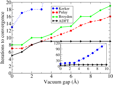
Figure 1: (Color online) Convergence of the bosonic ADFT scheme compared to the Pulay, Broyden and Kerker (inset) density mixing methods for a 2D slab of MgO as the vacuum gap between periodic slab images is varied.

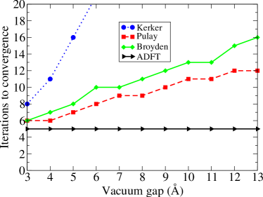
Figure 2: (Color online) Performance of the bosonic ADFT scheme for graphene, as a function of the spacing between periodic images in the perpendicular direction. The number of iterations taken to converge is approximately constant, whereas the iteration count for conventional density mixing methods grows.

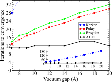
Figure 3: (Color online) Performance of the bosonic ADFT scheme compared to the Pulay, Broyden and Kerker (inset) density mixing methods for a gold nanoparticle, as a function of the spacing between periodic images.

In conclusion, an auxiliary density functional theory framework is introduced that maps the fermionic Kohn-Sham system onto an auxiliary system, which is not constrained to be fermionic. This mapping is constructed dynamically during an ordinary Kohn-Sham DFT calculation, and can be used to accelerate the convergence of SCF calculations considerably. The power of this ADFT framework is illustrated using a bosonic auxiliary system and the performance shown to be invariant with the size of the simulation cell, eliminating the ‘sloshing’ instabilities common in other techniques and removing the linear scaling of iteration count with system size. The method has been implemented in a development version of the CASTEP computer program, and demonstrates significantly superior performance to existing methods for a variety of systems from a wide-band-gap polar oxide thin film, to a 2D Dirac semi-metal and an isolated nanocluster.

The authors would like to thank M. J. Verstraete, M. Stankovski, H. Ness, J. D. Ramsden, M. J. P. Hodgson, K. Burke, M. Levy and especially R. W. Godby for many useful discussions. Financial support from the EPSRC and the United Kingdom Car-Parrinello Consortium is acknowledged with gratitude.

References

- (1) P. Hohenberg and W. Kohn, Phys. Rev. 136 864B (1964)
- (2) V. Milman, K. Refson, S.J. Clark, C.J. Pickard, J.R. Yates, S.P. Gao, P.J. Hasnip, M.I.J. Probert, A. Perlov and M.D. Segall, Journal of Molecular Structure: THEOCHEM 954 (1-3) 22-35 (2010).
- (3) P.J. Hasnip, K. Refson, M.I.J. Probert, J.R. Yates, S.J. Clark, C.J. Pickard, Phil. Trans. R. Soc. A 20130270 (2014)
- (4) M. Levy, Proceedings of the National Academy of Sciences 76 (12): 6062–6065 (1979)
- (5) W. Kohn and L.J. Sham, Phys. Rev. 140 1133A (1965)
- (6) P. Pulay, Chem. Phys. Lett. 73 393-398 (1980)
- (7) C.G. Broyden, Math. Comput. 19 577 (1965)
- (8) K.-M. Ho, J. Ihm and J.D. Joannopoulos, Phys. Rev. B 25 (6) 4260 (1982)
- (9) G.P. Kerker, Phys. Rev. B 23 3082 (1981)
- (10) M. Manninen, R. Nieminen and P. Hautojävri, Phys. Rev. B 12 4012 (1975)
- (11) G. Kresse and J. Furthmüller, Phys. Rev. B 54 11169 (1996)
- (12) E. Krotscheck and M. Liebrecht, J. Chem. Phys. 138 164114 (2013)
- (13) D. Raczkowski, A. Canning, and L. W. Wang, Phys. Rev. B 64 121101 (2001)
- (14) M.J.P. Hodgson, J.D. Ramsden, T.R. Durrant and R.W. Godby, Phys. Rev. B90 241107 (2014)
- (15) P.J. Hasnip and C.J. Pickard, Comp. Phys. Comm.174 pp. 24-29 (2006)
- (16) S.J. Clark, M.D. Segall, C.J. Pickard, P.J. Hasnip, M.J. Probert, K. Refson and M.C. Payne, Z. Kristallogr. 220(5-6) pp. 567-570 (2005)
- (17) K. P. McKenna and J. Blumberger, Phys. Rev. B 86 245110 (2012)
- (18) Vlado K. Lazarov, Zhuhua Cai, Kenta Yoshida, K. Honglian L. Zhang, M. Weinert, Katherine S. Ziemer and Philip J. Hasnip, Phys. Rev. Lett. 107 056101 (2011)
- (19) V.K. Lazarov, P.J. Hasnip, Z. Cai, K. Yoshida and K.S. Ziemer, J. Appl. Phys. 111 07A515 (2012)
- (20) Y. Hancock, J. Phys. D: Appl. Phys. 44 473001 (2011)
- (21) Y. Hancock, A. Uppstu, K. Saloriutta, A. Harju and M.J. Puska, Physical Review B 81 245402 (2010)
- (22) K. Saloriutta, Y. Hancock, A. Kärkkäinen, L. Kärkkäinen, M.J. Puska and A.-P. Jauho, Physical Review B 83 205125 (2011)
- (23) T. Fujita, P. Guan, K. P. McKenna, X. Lang, A. Hirata, L. Zhang, T. Tokunaga, S. Arai, Y. Yamamoto, N. Tanaka, Y. Ishikawa, N. Asao, Y. Yamamoto, J. Erlebacher and M. Chen Nature Materials 11 775-780 (2012)