Algorithms and Models for Turbulence Not at Statistical Equilibrium

Abstract

Standard eddy viscosity models, while robust, cannot represent backscatter and have severe difficulties with complex turbulence not at statistical equilibrium. This report gives a new derivation of eddy viscosity models from an equation for the evolution of variance in a turbulent flow. The new derivation also shows how to correct eddy viscosity models. The report proves the corrected models preserve important features of the true Reynolds stresses. It gives algorithms for their discretization including a minimally invasive modular step to adapt an eddy viscosity code to the extended models. A numerical test is given with the usual and over diffusive Smagorinsky model. The correction (scaled by $10^{-8}$ ) does successfully exhibit intermittent backscatter.

1 Introduction

Eddy viscosity models are the workhorses of practical turbulent flow simulations, [6]. Due to the wide experience with them, their limitations are also well recognized. They cannot represent backscatter (intermittent energy flow from turbulent fluctuations back to the mean velocity) without ad hoc fixes (called ”absurdities” in [23]) like negative viscosities. This report shows how to correct eddy viscosity models systematically to include backscatter based on a new and fundamental derivation of eddy viscosity models.

To begin, given an ensemble of initial conditions

$$u(x,0;\omega_{j})=u_{0}(x;\omega_{j}),j=1,\cdot\cdot\cdot,J,\text{ }x\in\Omega,$$

let $u(x,t;\omega_{j}),p(x,t;\omega_{j})$ be associated solutions to the Navier-Stokes equations (NSE)

$$u_{t}+u\cdot\nabla u-\nu\triangle u+\nabla p = f(x,t)\text{, and }\nabla\cdot u=0\text{, in }\Omega,$$ (1)

$$u = 0\text{ on }\partial\Omega\text{.}$$

Let $\left\langle\cdot\right\rangle$ denote ensemble averaging

$$\left\langle u\right\rangle(x,t):=\frac{1}{J}\sum_{j=1}^{J}u(x,t;\omega_{j})\text{ and }u^{\prime}(x,t;\omega_{j})=u(x,t;\omega_{j})-\left\langle u\right\rangle(x,t).$$

Ensemble averaging the NSE yields the non-closed system: $\nabla\cdot\left\langle u\right\rangle=0$ and

$$\left\langle u\right\rangle_{t}+\left\langle u\right\rangle\cdot\nabla\left\langle u\right\rangle-\nu\triangle\left\langle u\right\rangle-\nabla\cdot R(u,u)+\nabla\left\langle p\right\rangle=f(x,t)\text{,}$$ (2)

where the Reynolds stress $R(u,u)$ is

$$R(u,u):=\left\langle u\right\rangle\otimes\left\langle u\right\rangle-\left\langle u\otimes u\right\rangle=-\left\langle u^{\prime}\otimes u^{\prime}\right\rangle,$$

e.g., [2], [6], [23]. Statistical models of turbulence begin with ensemble averaging and replace $R(u,u)$ by an enhanced viscous term depending only on the mean velocity. We show in Section 2 that these eddy viscosity models are based on three steps.

1. The Boussinesq assumption (from [4], [26], proven in [18]) that turbulent fluctuations (the action of $\nabla\cdot R(u,u)$ in (2)) are dissipative on average in (2). This is followed by assuming that space and time averaged dissipativity holds pointwise in time and space.

2. The eddy viscosity hypothesis that this dissipativity aligns with the gradient or deformation tensor and thus can be represented by a viscous term with a turbulent viscosity coefficient $\nu_{T}(\left\langle u\right\rangle)$, [25].

3. Model parametrization/calibration is done by fitting the turbulent viscosity coefficient $\nu_{T}(\left\langle u\right\rangle)$ to flow data. Calibration is equivalent to specifying a fluctuation model for $\nabla u^{\prime}$ in terms of $\nabla\left\langle u\right\rangle$.

The resulting eddy viscosity model (whose solution $w(x,t)$, $q(x,t)$ is intended to be an approximation of the true flow averages $\left\langle u\right\rangle,\left\langle p\right\rangle$) results: $\nabla\cdot w=0$ and

$$w_{t}+w\cdot\nabla w-\nabla\cdot\left(\left[\nu+\nu_{T}(w)\right]\nabla w\right)+\nabla q=f(x,t)\text{, in }\Omega,$$ (EV)

$$w=0\text{ on }\partial\Omega\text{\ and }w(x,0)=\left\langle u_{0}\right\rangle\text{ in }\Omega\text{.}$$

Eddy viscosity models, with increasingly complex equations determining $\nu_{T}(w)$, are the models of choice for most industrial turbulent flows, [6], and many parameterizations of eddy viscosity models are known, e.g., [3], [5] [12], [13], [19], [20], [22], [31]. They have well recognized limitations in not modeling complex turbulence, backscatter or turbulence not at statistical equilibrium, e.g., [8], [21], [27], [30]. (The second assumption that the dissipativity of the Reynolds stress term aligns with $\nabla\left\langle u\right\rangle$ also fails for some flows, [21], but is not the issue addressed herein.)

The correction required for eddy viscosity models to represent backscatter in non-statistically stationary turbulence, the case when the action of the fluctuations is intermittently non-dissipative, is derived and analyzed herein. Given the eddy viscosity parameterization $\nu_{T}(w),$ choose a re-scaling parameter $\beta>0$ and define

$$a(w):=\sqrt{\nu^{-1}\nu_{T}(w)}.$$

The corrected EV model (derived in Section 2) is then $\nabla\cdot w=0$ and

$$w_{t}+\beta^{2}a(w)\frac{\partial}{\partial t}\left(a(w)w\right)+w\cdot\nabla w$$ (Corrected EV)

$$-\nabla\cdot\left(\left[\nu+\nu_{T}(w)\right]\nabla w\right)+\nabla q=f(x,t)\text{.}$$

In Section 3 time averaged dissipativity, an important feature of the true Reynolds stresses, is proven to be preserved in (Corrected EV).

The (Corrected EV) differs from (EV) by the extra term $\beta^{2}a(w)\frac{\partial}{\partial t}\left(a(w)w\right)$. This term means time discretization introduces new issues, especially in adapting legacy codes from (EV) to (Corrected EV). Section 4 shows how time discretization can be done and preserve these important model properties, including the important case of modular adaptation of a legacy code available for (EV). Phenomenology is used to obtain some insight into calibration of the re-scaling parameter $\beta$ in Section 5. Section 6 tests correction of the over-diffused Smagorinsky model. Even with a very small rescaling of the correction, $\beta^{2}\simeq O(10^{-8})$, the numerical test shows that the corrected model does exhibit backscatter.

2 Derivation of Corrected EV Models

Beginning with two results from [18], this section shows that eddy viscosity models are based on three assumptions and that they are only consistent in a time averaged sense. Next we show how to take a given eddy viscosity model and extend it to be energy consistent with the NSE pointwise in time.

The ensemble averaged Navier Stokes equations, (2) above, involve the non-closed Reynolds stress $R(u,u)=-\left\langle u^{\prime}\otimes u^{\prime}\right\rangle$. This term, which must be modelled, accounts for the effects of the fluctuations on the mean flow, e.g., [5], [6], [22], [25], [28]. Let $||\cdot||,(\cdot,\cdot)$ denote the usual $L^{2}(\Omega)$ norm and inner product. Taking the inner product of (2) with $\left\langle u\right\rangle$ and performing the usual steps gives the equation for the kinetic energy evolution of $\left\langle u\right\rangle$:

$$\frac{d}{dt}\frac{1}{2}||\left\langle u\right\rangle||^{2}+\nu||\nabla\left\langle u\right\rangle||^{2}+\int_{\Omega}R(u,u):\nabla\left\langle u\right\rangle dx=(f,\left\langle u\right\rangle).$$

Thus, the effect of fluctuations on the mean flow is determined by the sign of

$$RS(t):=\int_{\Omega}R(u,u):\nabla\left\langle u\right\rangle dx.$$

When $RS(t)>0$, the effect of $R(u,u)$ is dissipative while when $RS(t)<0$, (volume averaged) backscatter occurs and fluctuations increase the energy in the mean flow. In [18], [15], two key properties of this Reynolds stress term were proven: time averaged dissipativity and an equation for the evolution of variance of fluctuations:

$$LIM_{T\rightarrow\infty}\frac{1}{T}\int_{0}^{T}RS(t)dt=LIM_{T\rightarrow\infty}\frac{1}{T}\int_{0}^{T}\int_{\Omega}\nu\left\langle|\nabla u^{\prime}|^{2}\right\rangle dxdt\geq 0,$$ (3)

$$\int_{\Omega}R(u,u):\nabla\left\langle u\right\rangle dx=\frac{1}{2}\frac{d}{dt}\int\left\langle u^{\prime}\cdot u^{\prime}\right\rangle dx+\nu\int\left\langle\nabla u^{\prime}:\nabla u^{\prime}\right\rangle dx.$$ (4)

Eddy viscosity models then follow from three assumptions. First, the statistical equilibrium assumption that dissipativity holds approximately at every instant in time

$$\int_{\Omega}R(u,u):\nabla\left\langle u\right\rangle dx\simeq\int_{\Omega}\nu\left\langle|\nabla u^{\prime}|^{2}\right\rangle dx.$$ (5)

The second is that $\nabla u^{\prime}$ aligns with $\nabla\left\langle u\right\rangle$. Third, calibration provides a model of the fluctuations in terms of the mean flow

$$action(\nabla u^{\prime})\simeq a(\left\langle u\right\rangle)\nabla\left\langle u\right\rangle.$$ (6)

Thus,

$$\int_{\Omega}R(u,u):\nabla\left\langle u\right\rangle dx\simeq\int_{\Omega}\nu a(\left\langle u\right\rangle)^{2}\nabla\left\langle u\right\rangle:\nabla\left\langle u\right\rangle dx$$

$$=\int_{\Omega}-\nabla\cdot\left(\nu a(\left\langle u\right\rangle)^{2}\nabla\left\langle u\right\rangle\right)\cdot vdx\text{ evaluated at }v=\left\langle u\right\rangle.$$

Letting $\nu_{T}(\left\langle u\right\rangle)=\nu a(\left\langle u\right\rangle)^{2}$, this yields the eddy  viscosity closure

$$-\nabla\cdot R(u,u)\text{ }\Leftarrow\text{ }-\nabla\cdot\left(\nu_{T}(\left\langle u\right\rangle)\nabla\left\langle u\right\rangle\right)+\text{ terms incorporated in }\nabla p\text{.}$$

Far from equilibrium, step (5) omits $\frac{1}{2}\frac{d}{dt}\int\left\langle u_{j}^{\prime}\cdot u_{j}^{\prime}\right\rangle dx$ in (4). This is the term that accounts for backscatter and other non-equilibrium effects. To model this term, $u^{\prime}$ must be expressed in terms of $\left\langle u\right\rangle$. For this, the simplest (explored herein) is to rescale (by $\beta$, Section 4) the fluctuation model (6), yielding

$$action(u^{\prime})\simeq\beta a(\left\langle u\right\rangle)\left\langle u\right\rangle$$

This assumption yields

$$\int R(u,u):\nabla\left\langle u\right\rangle dx\simeq\frac{1}{2}\frac{d}{dt}\int\beta^{2}a(\left\langle u\right\rangle)^{2}|\left\langle u\right\rangle(x,t)|^{2}dx+\int\nu a(\left\langle u\right\rangle)^{2}|\nabla\left\langle u\right\rangle(x,t)|^{2}dx,$$

arising from an anisotropic time derivative $\beta^{2}a(\left\langle u\right\rangle)\frac{\partial}{\partial t}\left(a\left\langle u\right\rangle)\left\langle u\right\rangle\right)$ and an eddy viscosity term $-\nabla\cdot\left(\nu_{T}(\left\langle u\right\rangle)\nabla\left\langle u\right\rangle\right)$ where $\nu_{T}(\left\langle u\right\rangle)=\nu a(\left\langle u\right\rangle)^{2}.$ This gives the closure model

$$-\nabla\cdot R(u,u)\simeq\beta^{2}a(\left\langle u\right\rangle)\frac{\partial}{\partial t}\left(a(\left\langle u\right\rangle)\left\langle u\right\rangle\right)-\nabla\cdot\left(\nu_{T}\left\langle u\right\rangle)\nabla\left\langle u\right\rangle\right)$$

and thus we have the corrected model: $\nabla\cdot w=0$ and

$$\ w_{t}+\beta^{2}a(w)\frac{\partial}{\partial t}\left(a(w)w\right)+w\cdot\nabla w+\nabla p-\nabla\cdot\left([\nu+\nu_{T}(w)]\nabla w\right)=f\text{ }.$$ (7)

3 Analysis of The Corrected Smagorinsky Model

The classic example of an over-diffused model is the standard Smagorinsky model for which

$$\nu_{T}(w)=\left(C_{s}\delta\right)^{2}|\nabla w|,\text{ \ where \ }C_{s}\simeq 0.1,\delta=\triangle x.$$

(Other numerical values of $C_{s}$ are also used, [29] Table 1.) Various fixes for it include van Driest damping (reducing near wall model dissipation) and Germano’s dynamic selection of $\mu=C_{s}^{2}(x,t)$. These are often successful but the latter leads to negative values of $\mu$ that model backscatter but can induce instabilities. Often these are clipped ($\mu\Leftarrow\max\{\mu,0\}$) eliminating backscatter being represented in the model.

In this section we prove that the corrected Smagorinsky model preserves the property of the true turbulent fluctuations that on long time average they are dissipative, Theorem 3.2. For the Smagorinsky model we have

$$\nu_{T}(w)=\left(C_{s}\delta\right)^{2}|\nabla w|,\text{ and thus }a(w)=\nu^{-1/2}C_{s}\delta\sqrt{|\nabla w|}.$$

Let $\beta>0$, $a(w)=\nu^{-1/2}C_{s}\delta\sqrt{|\nabla w|}$ and consider

$$\left.\begin{array}[]{c}\ w_{t}+\beta^{2}a(w)\frac{\partial}{\partial t}\left(a(w)w\right)+w\cdot\nabla w+\nabla p-\nabla\cdot\left([\nu+\nu_{T}(w)]\nabla w\right)=f,\\ \text{ }\nabla\cdot w=0\text{ in }\Omega\times(0,\infty),\\ w=0\text{ on }\partial\Omega,w(x,0)=w_{0}(x),\text{ in }\Omega.\end{array}\right\}$$ (8)

The model dissipation function for the effect of the model of the Reynolds stresses on the kinetic energy in the mean flow will be denoted by

$$MD(t):=\int_{\Omega}\beta^{2}a(w)\frac{\partial}{\partial t}\left(a(w)w\right)\cdot w+\nu_{T}(w)|\nabla w|^{2}dx.$$

The numerical tests in Section 6 establish (Figure 6.2) that, even for very small $\beta$, the extra term does allow the sign of the model dissipation $MD(t)$ to fluctuate. We prove the time average of $MD(t)$ is non-negative.

We assume

$$f(x,t)\in L^{\infty}(0,\infty;L^{2}(\Omega)),w_{0}(x)\in L^{2}(\Omega),$$

$$w\text{ is a strong solution of (3.1).}$$

Lemma 1.

For $a(w)=\nu^{-\frac{1}{2}}C_{s}\delta\sqrt{|\nabla w|}$ we have for all $w\in\mathring{W}^{1,3}(\Omega)$

$$||a(w)w||^{2}\leq C(\Omega)\nu^{-1}\left(C_{s}\delta\right)^{2}||\nabla w||_{L^{3}}^{3}.$$

Proof.

By Hölder’s inequality and the Poincaré-Friedrichs inequality

$$||a(w)w||^{2}=\nu^{-1}\left(C_{s}\delta\right)^{2}\int_{\Omega}|\nabla w||w|^{2}dx$$

$$\leq\nu^{-1}\left(C_{s}\delta\right)^{2}||w||_{L^{3}}^{2}||\nabla w||_{L^{3}}\leq C(\Omega)\nu^{-1}\left(C_{s}\delta\right)^{2}||\nabla w||_{L^{3}}^{3}.$$

   

We prove next that $MD(t)$ dissipates energy in the time average sense.

Theorem 2.

Let $C_{s}>0,\delta>0,\beta>0$ and $w$ be a strong solution of (8). Then

$$w\text{ , }a(w)w \in L^{\infty}(0,\infty;L^{2}(\Omega)),$$ (9)

$$\frac{1}{T}\int_{0}^{T}\left(\int_{\Omega}\left[\nu+\nu_{T}(w\right])\nabla w:\nabla wdx\right)dt \leq C<\infty,\text{ }C\text{ independent of }T\text{.}$$ (10)

The model also satisfies long term balance between energy input and dissipation: for any generalized limit $LIM$

$$\ LIM_{T\rightarrow\infty}\frac{1}{T}\int_{0}^{T}\left(\int_{\Omega}\left[\nu+\nu_{T}(w\right])|\nabla w|^{2}dx\right)dt=LIM_{T\rightarrow\infty}\frac{1}{T}\int_{0}^{T}(f,w)dt.$$

Further

$$0\leq\lim_{T\rightarrow\infty}\inf\frac{1}{T}\int_{0}^{T}MD(t)dt\leq\lim_{T\rightarrow\infty}\sup\frac{1}{T}\int_{0}^{T}MD(t)dt<\infty.$$

Proof.

Take the inner product of the corrected Smagorinsky model with $w$. This yields

$$\ \frac{1}{2}\frac{d}{dt}\left[||w||^{2}+\beta^{2}||a(w)w||^{2}\right]+\int_{\Omega}\left[\nu+\nu_{T}(w)\right]|\nabla w|^{2}dx=(f,w).$$ (11)

Let

$$F:=\frac{1}{2\nu}||f||_{L^{\infty}(0,\infty;L^{2}(\Omega))}\text{ \ and \ }y(t):=\ \frac{1}{2}\left[||w||^{2}+\beta^{2}||a(w)w||^{2}\right].$$

By Lemma 3.1,

$$2y(t) = ||w||^{2}+\beta^{2}||a(w)w||^{2}\leq C\left(\int_{\Omega}\left[\nu+\nu_{T}(w)\right]|\nabla w|^{2}dx\right)$$

$$\leq C\left(\nu||\nabla w||^{2}+\left(C_{s}\delta\right)^{2}||\nabla w||_{L^{3}}^{3}\right).$$

Since $(f,w)\leq\frac{\nu}{2}||\nabla w||^{2}+\frac{1}{2\nu}||f||_{-1}^{2}$, $y(t)$ thus satisfies

$$y^{\prime}(t)+\alpha y(t)\leq F(<\infty)\text{ for some }\alpha>0.$$

This implies $y(t)\in\ L^{\infty}(0,\infty)$ which is the first claimed á priori bound. This bound now implies that $(f,w)(t)\in L^{\infty}(0,\infty).$ Integrating (11) over $[0,T]$ and dividing by $T$ gives

$$\ \frac{1}{2T}\left[||w||^{2}+\beta^{2}||a(w)w||^{2}\right](T)+\frac{1}{T}\int_{0}^{T}\left(\int_{\Omega}\left[\nu+\nu_{T}(w\right])|\nabla w|^{2}dx\right)dt$$ (12)

$$=\frac{1}{2T}\left[||w_{0}||^{2}+\beta^{2}||a(w_{0})w_{0}||^{2}\right]+\frac{1}{T}\int_{0}^{T}(f,w)dt.$$

Since $(f,w)\in L^{\infty}(0,\infty)$ this implies (10) holds which implies as $T\rightarrow\infty$  limit inferiors and superiors exist. The á priori estimates (9), (10) imply that (12) takes the form

$$\ \mathcal{O}(\frac{1}{T})+\frac{1}{T}\int_{0}^{T}\left(\int_{\Omega}\left[\nu+\nu_{T}(w\right])|\nabla w|^{2}dx\right)dt=\mathcal{O}(\frac{1}{T})+\frac{1}{T}\int_{0}^{T}(f,w)dt.$$ (13)

Letting $T\rightarrow\infty$ implies long term balance between energy input and dissipation.

Consider now the time average of $MD(t)$. We have

$$\frac{1}{T}\int_{0}^{T}MD(t)dt = \frac{1}{T}\int_{0}^{T}\int_{\Omega}\left[\beta^{2}\frac{\partial}{\partial t}\left(a(w)w\right)\cdot(a(w)w)+\nu_{T}(w)|\nabla w|^{2}\right]dxdt$$

$$= \frac{1}{T}\int_{0}^{T}\left[\frac{\beta^{2}}{2}\frac{d}{dt}||a(w)w||^{2}+\left(C_{s}\delta\right)^{2}||\nabla w||_{L^{3}}^{3}\right]dt$$

$$= \frac{\beta^{2}}{2T}\left(||a(w(T))w(T)||^{2}-||a(w(0))w(0)||^{2}\right)+\frac{1}{T}\int_{0}^{T}\left(C_{s}\delta\right)^{2}||\nabla w||_{L^{3}}^{3}dt.$$

From (12), the right hand side equals

$$\frac{1}{T}\int_{0}^{T}MD(t)dt=\frac{1}{T}\int_{0}^{T}(f,w)dt-\frac{1}{T}\int_{0}^{T}\nu||\nabla w||^{2}dt-\frac{1}{2T}\left[||w||^{2}(T)-||w_{0}||^{2}\right],$$

while from (13) we have

$$\frac{1}{T}\int_{0}^{T}MD(t)dt = \frac{1}{T}\int_{0}^{T}(f,w)dt-\frac{1}{T}\int_{0}^{T}\nu||\nabla w||^{2}dt$$

$$= \ \mathcal{O}(\frac{1}{T})-\mathcal{O}(\frac{1}{T})+\frac{1}{T}\int_{0}^{T}\left(C_{s}\delta\right)^{2}||\nabla w||_{L^{3}}^{3}dt.$$

Thus the limit inferior of the time average of $MD(t)$ exists and is non-negative.    

4 Time Discretization of Corrected Eddy Viscosity Models

This section presents three unconditionally stable, linearly implicit time discretizations of (Corrected EV). Method 1 and the modular Method 2 are first order accurate. Method 3 is second order accurate. All three preserve the essential feature of time averaged dissipativity, Proposition 4.3. The second method shows how a legacy code for solving (EV) can be adapted to solve (Corrected EV). We suppress the spacial discretization to reduce notation and focus on essential points. Let the timestep and associated quantities be denoted as usual by

$$\text{timestep}=k,\text{ \ \ }t_{n}=nk,\text{ \ \ }f^{n}(x):=f(x,t_{n}),$$

$$w^{n}(x)=\text{ approximation to }w(x,t_{n}),\text{ and }a^{n}:=a(w^{n}),\text{ \ \ }\nu_{T}^{n}:=\nu_{T}(w^{n}),n\geq 0,$$

and set $a^{-1}=a^{0}=a(w^{0})$. We consider time discretization of  (Corrected EV) under no-slip boundary conditions. The first method is: given $w^{0},$ find $w^{n}$ satisfying

$$\frac{w^{n+1}-w^{n}}{k}+\beta^{2}a^{n}\frac{a^{n}w^{n+1}-a^{n-1}w^{n}}{k}$$

$$+w^{n}\cdot\nabla w^{n+1}-\nabla\cdot\left(\left[\nu+\nu_{T}^{n}\right]\nabla w^{n+1}\right)+\nabla q^{n+1}=f^{n+1}(x)\text{ in }\Omega,$$ (Method 1)

$$\nabla\cdot w^{n+1}=0\text{ in }\Omega,\text{ and }w^{n+1}=0\text{ on }\partial\Omega\text{ .}$$

This method is linearly implicit. We shall prove in Theorem 4.1 that it is unconditionally, nonlinearly stable. In linearly implicit methods (considered herein) nonlinearities are lagged to previous time levels (or extrapolated), so there is no difficulty if $\nu_{T}$ is determined by solving other nonlinear equations, such as in the $k-\varepsilon$ model, [5], [22].

Comparing the model, this method and the ensemble averaged NSE, we see that

1. True effect of fluctuations on means: $RS(t)=$ $\int_{\Omega}R(u,u):\nabla\left\langle u\right\rangle dx.$

2. Model: $MD(t)=$ $\int_{\Omega}\beta^{2}a(w)\frac{\partial}{\partial t}\left(a(w)w\right)\cdot w+\nu_{T}(w)|\nabla w|^{2}dx,$

3. Discrete version: $MD^{n+1}=$ $\int_{\Omega}\beta^{2}a^{n}\frac{a^{n}w^{n+1}-a^{n-1}w^{n}}{k}\cdot w^{n+1}+\nu_{T}^{n}|\nabla w^{n+1}|^{2}dx$.

Theorem 3.

(Method 1) is unconditionally, nonlinearly energy stable. For any $N\geq 1$

$$\left(\frac{1}{2}||w^{N}||^{2}+\frac{1}{2}\beta^{2}||a^{N-1}w^{N}||^{2}\right)$$

$$+\sum_{n=0}^{N-1}\frac{1}{2}\left(||w^{n+1}-w^{n}||^{2}+\beta^{2}||a^{n}w^{n+1}-a^{n-1}w^{n}||^{2}\right)$$

$$+k\sum_{n=0}^{N-1}\int_{\Omega}\left[\nu+\nu_{T}^{n}\right]|\nabla w^{n+1}|^{2}dx$$

$$=\left(\frac{1}{2}||w^{0}||^{2}+\frac{1}{2}\beta^{2}||a^{-1}w^{0}||^{2}\right)+k\sum_{n=0}^{N-1}(f^{n+1},w^{n+1}).$$

Proof.

Multiply through by $k$, take the $L^{2}$ inner product of (Method 1) with $w^{n+1}$ and use $(w^{n}\cdot\nabla w^{n+1},w^{n+1})=0$. This gives

$$||w^{n+1}||^{2}-(w^{n+1},w^{n})+\beta^{2}||a^{n}w^{n+1}||^{2}-\beta^{2}(a^{n-1}w^{n},a^{n}w^{n+1})$$

$$+k\int_{\Omega}\left[\nu+\nu_{T}^{n}\right]|\nabla w^{n+1}|^{2}dx=k\int_{\Omega}f^{n+1}\cdot w^{n+1}dx.$$

The second and fourth terms are treated by the polarization identity

$$(w^{n+1},w^{n}) = \frac{1}{2}||w^{n+1}||^{2}+\frac{1}{2}||w^{n}||^{2}-\frac{1}{2}||w^{n+1}-w^{n}||^{2},$$

$$(a^{n-1}w^{n},a^{n}w^{n+1}) = \frac{1}{2}||a^{n}w^{n+1}||^{2}+\frac{1}{2}||a^{n-1}w^{n}||^{2}-\frac{1}{2}||a^{n}w^{n+1}-a^{n-1}w^{n}||^{2}.$$

Collecting terms and summing from $n=0$ to $N-1$ finishes the proof.    

Since Theorem 4.1 is an energy equality we can identify various effects:

• Model kinetic energy = $\frac{1}{2}||w^{N}||^{2}+\frac{1}{2}\beta^{2}||a^{N-1}w^{N}||^{2}$

• model dissipation = $\int_{\Omega}\nu_{T}^{n}|\nabla w^{n+1}|^{2}dx$

• numerical diffusion = $\frac{1}{2}\left(||w^{n+1}-w^{n}||^{2}+\beta^{2}||a^{n}w^{n+1}-a^{n-1}w^{n}||^{2}\right).$

Rewriting the energy equality in an equivalent form gives

$$\frac{1}{2k}\left(||w^{n+1}||^{2}-||w^{n}||^{2}\right)+\frac{1}{2k}||w^{n+1}-w^{n}||^{2}+\nu||\nabla w^{n+1}||^{2}+$$

$$\left\{\frac{\beta^{2}}{2k}\left(||a^{n}w^{n+1}||^{2}-||a^{n-1}w^{n}||^{2}\right)+\frac{\beta^{2}}{2k}||a^{n}w^{n+1}-a^{n-1}w^{n}||^{2}+\int_{\Omega}\nu_{T}^{n}|\nabla w^{n+1}|^{2}dx\right\}$$

$$=(f^{n+1},w^{n+1}).$$

The first and last line arise from the terms in the usual backward Euler discretization of the NSE. The second line (bracketed) is an equivalent form of $MD^{n+1}.$

Lemma 4.

For (Method 1) we have

$$MD^{n+1}=\frac{\beta^{2}}{2k}\left(||a^{n}w^{n+1}||^{2}-||a^{n-1}w^{n}||^{2}\right)$$

$$+\frac{\beta^{2}}{2k}||a^{n}w^{n+1}-a^{n-1}w^{n}||^{2}+\int_{\Omega}\nu_{T}^{n}|\nabla w^{n+1}|^{2}dx.$$

Dissipativity on time average holds for all three methods with the same manipulations of their discrete energy equality. We record it here for (Method 1).

Proposition 5 (Time Averaged Dissipativity).

Suppose $\sup_{0<n<\infty}||f(t^{n})||<\infty$. Then, for $T_{N}=N\triangle t,$

$$\lim\inf_{T_{N}\rightarrow\infty}\frac{1}{T_{N}}\left(\triangle t\sum_{n=0}^{N}MD^{n+1}\right)\geq 0.$$

Proof.

The proof is a discrete analog of the continuous case and will be omitted.    

4.1 Modular Correction of EV Models

Given a code that computes an approximation to the EV model

$$w_{t}+w\cdot\nabla w-\nabla\cdot\left(\left[\nu+\nu_{T}(w)\right]\nabla w\right)+\nabla q=f(x,t)\text{.}$$ (14)

Algorithm 4.2 presents a minimally intrusive, modular, postprocessor to solve:

$$w_{t}+\beta^{2}a(w)\frac{\partial}{\partial t}\left(a(w)w\right)+w\cdot\nabla w-\nabla\cdot\left(\left[\nu+\nu_{T}(w)\right]\nabla w\right)+\nabla q=f(x,t)\text{.}$$ (15)

Precise stability analysis requires a specific choice of the algorithm used to solve (14). For this we select the simple, linearly implicit, backward Euler method.

Derivation and Consistency Error. To derive the modular postprocessor, rewrite (14) and (15) as, respectively,

$$y^{\prime}(t)=f(t,y)\text{ \ and \ }y^{\prime}(t)+\beta^{2}a(y)\frac{d}{dt}(a(y)y)=f(t,y).$$

The postprocessing given in Step 2 below suffices.

Algorithm 6 (Method 2).

Given  $y^{n},y^{n-1},$

Step 1: Calculate $y_{temp}^{n+1}$ by:   $\frac{y_{temp}^{n+1}-y^{n}}{k}=f(t_{n+1},y_{temp}^{n+1}),$

Step 2 : Postprocess to obtain $y^{n+1}$ from $y_{temp}^{n+1}$ by:

$\left[1+\beta^{2}a(y^{n})^{2}\right]y^{n+1}=y_{temp}^{n+1}+\beta^{2}a(y^{n})a(y^{n-1})y^{n}$ .

Eliminating $y_{temp}^{n+1}$ from Step 2 shows that $y^{n+1}$ satisfies (with $a^{n}=a(y^{n})$)

$$\frac{y^{n+1}-y^{n}}{k}+\beta^{2}a^{n}\frac{a^{n}y^{n+1}-a^{n-1}y^{n}}{k}=f(t_{n+1},y_{temp}^{n+1}).$$

Although this is close to Method 1, $y_{temp}^{n+1}$ not $y^{n+1}$ occurs in the RHS. The LHS is clearly a first order approximation to $y^{\prime}(t)+\beta a(y)(a(y)y)^{\prime}$. The RHS, $f(t_{n+1},y_{temp}^{n+1})$, is a first order approximation to $f(t,y)$ provided $y_{temp}^{n+1}-y^{n+1}=O(k)$. Rearranging Step 2 gives

$$y_{temp}^{n+1}-y^{n+1} = k\left\{\beta^{2}a(y^{n})\frac{a(y^{n})y^{n+1}-a(y^{n-1})y^{n}}{k}\right\}$$

$$= k\left(\beta^{2}a(y)\frac{d}{dt}(a(y)y)\right)+O(k^{2})=O(k).$$

Thus, Algorithm 4.4 is first order accurate approximation of $y^{\prime}(t)+\beta^{2}a(y)(a(y)y)^{\prime}$ = $f(t,y)$.

Unconditional Stability of the Modular Algorithm. The utility of Algorithm 4.4 thus depends on its stability. This is now analyzed for its application to the corrected EV model. Algorithm 4.4 for (15) reads as follows.

Algorithm 7.

For $n\geq 0,$ given $w^{n}$

Step 1: Find $w_{temp}^{n+1}$ satisfying

$$\frac{w_{temp}^{n+1}-w^{n}}{k}+w^{n}\cdot\nabla w_{temp}^{n+1}$$

$$-\nabla\cdot\left(\left[\nu+\nu_{T}^{n}\right]\nabla w_{temp}^{n+1}\right)+\nabla q_{temp}^{n+1}=f^{n+1}(x)\text{ in }\Omega,$$

$$\nabla\cdot w_{temp}^{n+1}=0\text{ in }\Omega,\text{ and }w_{temp}^{n+1}=0\text{ on }\partial\Omega\text{ .}$$

Step 2: Given $w_{temp}^{n+1},q_{temp}^{n+1}$ find $w^{n+1},q^{n+1}$ satisfying

$$[1+\beta^{2}\left(a^{n}\right)^{2}]w^{n+1}+\nabla q^{n+1}=w_{temp}^{n+1}+\beta^{2}a^{n}a^{n-1}w^{n}\text{ in }\Omega$$ (16)

$$\nabla\cdot w^{n+1}=0\text{ in }\Omega,\text{ and }w^{n+1}=0\text{ on }\partial\Omega\text{ .}$$

We prove Algorithm 4.5 is unconditionally stable.

Theorem 8.

Algorithm 4.5 is unconditionally, nonlinearly energy stable. For any $N\geq 1$

$$\left(\frac{1}{2}||w^{N}||^{2}+\frac{1}{2}\beta^{2}||a^{N-1}w^{N}||^{2}\right)$$

$$+\sum_{n=0}^{N-1}\frac{1}{2}\left(||w^{n+1}-w_{temp}^{n+1}||^{2}+||w_{temp}^{n+1}-w^{n}||^{2}\right)$$

$$+k\sum_{n=0}^{N-1}\left(\int_{\Omega}\left[\nu+\nu_{T}^{n}\right]|\nabla w_{temp}^{n+1}|^{2}dx\right)$$

$$=\left(\frac{1}{2}||w^{0}||^{2}+\frac{1}{2}\beta^{2}||a^{-1}w^{0}||^{2}\right)+k\sum_{n=0}^{N-1}(f^{n+1},w_{temp}^{n+1}).$$

Proof.

Take the $L^{2}$ inner product of Step 1 with $w_{temp}^{n+1}$ and follow the proof of Theorem 1. This gives

$$\frac{1}{2}||w_{temp}^{n+1}||^{2}-\frac{1}{2}||w^{n}||^{2}+\frac{1}{2}||w_{temp}^{n+1}-w^{n}||^{2}$$ (Step 1 Energy)

$$+k\int_{\Omega}\left[\nu+\nu_{T}^{n}\right]|\nabla w_{temp}^{n+1}|^{2}dx=k(f^{n+1},w_{temp}^{n+1}).$$

Consider Step 2. Taking the $L^{2}$ inner product with $w^{n+1}$ gives

$$||w^{n+1}||^{2}+\beta^{2}||a^{n}w^{n+1}||^{2}=(w_{temp}^{n+1},w^{n+1})+\beta^{2}(a^{n-1}w^{n},a^{n}w^{n+1}).$$

The two terms on the RHS are treated with the polarization identity

$$(w_{temp}^{n+1},w^{n+1}) = \frac{1}{2}||w_{temp}^{n+1}||^{2}+\frac{1}{2}||w^{n+1}||^{2}-\frac{1}{2}||w_{temp}^{n+1}-w^{n+1}||^{2},$$

$$(a^{n-1}w^{n},a^{n}w^{n+1}) = \frac{1}{2}||a^{n}w^{n+1}||^{2}+\frac{1}{2}||a^{n-1}w^{n}||^{2}-\frac{1}{2}||a^{n}w^{n+1}-a^{n-1}w^{n}||,$$

giving

$$\frac{1}{2}||w^{n+1}||^{2}+\frac{1}{2}\beta^{2}||a^{n}w^{n+1}||^{2}-\frac{\beta^{2}}{2}||a^{n-1}w^{n}||^{2}+\frac{1}{2}||w_{temp}^{n+1}-w^{n+1}||^{2}$$

$$+\frac{\beta^{2}}{2}||a^{n}w^{n+1}-a^{n-1}w^{n}||=\frac{1}{2}||w_{temp}^{n+1}||^{2}.$$

Insert the LHS for $\frac{1}{2}||w_{temp}^{n+1}||^{2}$ in (Step 1 Energy). This gives

$$\frac{1}{2}||w^{n+1}||^{2}-\frac{1}{2}||w^{n}||^{2}+\frac{1}{2}\beta^{2}||a^{n}w^{n+1}||^{2}-\frac{1}{2}\beta^{2}||a^{n-1}w^{n}||^{2}$$

$$+\frac{1}{2}||w_{temp}^{n+1}-w^{n}||^{2}+\frac{1}{2}||w_{temp}^{n+1}-w^{n+1}||^{2}+\frac{\beta^{2}}{2}||a^{n}w^{n+1}-a^{n-1}w^{n}||^{2}$$

$$+k\int_{\Omega}\left[\nu+\nu_{T}^{n}\right]|\nabla w_{temp}^{n+1}|^{2}dx=k\int_{\Omega}f^{n+1}\cdot w_{temp}^{n+1}dx.$$

The result now follows by summing over $n$.    

A Second Order Time Discretization. We present a second order method comprised of an IMEX combination of BDF2 and AB2 adapted to the new kinetic energy term. It shortens the notation considerably to denote the linear extrapolation of a variable $\phi$ to $t^{n+1}$ by $\phi^{\ast n+1}:$

$$\phi^{\ast n+1}:=2\phi^{n}-\phi^{n-1},\text{ for }\phi=w,a,\nu_{T}.$$

The method is: given $w^{0}$, $w^{1}$, $w^{2}$ and $w^{3}$ (found by another method) find $w^{n+1}$  for $n\geq 3$ satisfying

$$\frac{3w^{n+1}-4w^{n}+w^{n-1}}{2k}$$ (Method 3)

$$+\beta^{2}a^{\ast n+1}\frac{3a^{\ast n+1}w^{n+1}-4a^{\ast n}w^{n}+a^{\ast n-1}w^{n-1}}{2k}$$

$$+w^{\ast n+1}\cdot\nabla w^{n+1}-\nabla\cdot\left(\left[\nu+\nu_{T}^{\ast n+1}\right]\nabla w^{n+1}\right)+\nabla q^{n+1}=f^{n+1}(x)\quad\text{in }\Omega,$$

$$\nabla\cdot w^{n+1}=0\text{ in }\Omega,\text{ and }w^{n+1}=0\text{ on }\partial\Omega\text{ .}$$

Theorem 9.

The method (Method 3) is unconditionally, nonlinearly, long time stable. For any $N\geq 3$

$$\frac{1}{4}\big{(}\|w^{N}\|^{2}+\|w^{\ast N+1}\|^{2}\big{)}$$

$$+\frac{1}{4}\Big{(}\beta^{2}\|a^{\ast N}w^{N}\|^{2}+\beta^{2}\|2a^{\ast N}w^{N}-a^{\ast N-1}w^{N-1}\|^{2}\Big{)}$$

$$+\sum_{n=3}^{N-1}\Big{\{}\frac{1}{4}\beta^{2}\|a^{\ast n+1}w^{n+1}-2a^{\ast n}w^{n}+a^{\ast n-1}w^{n-1}\|^{2}$$

$$+\frac{1}{4}\|w^{n+1}-2w^{n}+w^{n-1}\|^{2}+k\int_{\Omega}\left[\nu+\nu_{T}^{\ast n+1}\right]|\nabla w^{n+1}|^{2}dx\Big{\}}$$

$$=\sum_{n=3}^{N-1}k(f^{n+1},w^{n+1})+\frac{1}{4}\big{(}\|w^{3}\|^{2}+\|2w^{3}-w^{2}\|^{2}\big{)}$$

$$+\frac{1}{4}\Big{(}\beta^{2}\|a^{\ast 3}w^{3}\|^{2}+\beta^{2}\|2a^{\ast 3}w^{3}-a^{\ast 2}w^{2}\|^{2}\Big{)}.$$

Proof.

Take the $L^{2}$ inner product of (Method 3) with $w^{n+1}$ and multiply through by $k$. This gives

$$\frac{1}{4}\big{(}\|w^{n+1}\|^{2}+\|w^{\ast n+2}\|^{2}\big{)}-\frac{1}{4}\left(\|w^{n}\|^{2}+\|w^{\ast n+1}\|^{2}\right)$$

$$+\frac{1}{4}\Big{(}\beta^{2}\|a^{\ast n+1}w^{n+1}\|^{2}+\beta^{2}\|2a^{\ast n+1}w^{n+1}-a^{\ast n}w^{n}\|^{2}\Big{)}$$

$$-\frac{1}{4}\Big{(}\beta^{2}\|a^{\ast n}w^{n}\|^{2}+\beta^{2}\|2a^{\ast n}w^{n}-a^{\ast n-1}w^{n-1}\|^{2}\Big{)}$$

$$+\frac{1}{4}\beta^{2}\|a^{\ast n+1}w^{n+1}-2a^{\ast n}w^{n}+a^{\ast n-1}w^{n-1}\|^{2}$$

$$+\frac{1}{4}\|w^{n+1}-2w^{n}+w^{n-1}\|^{2}+k\int_{\Omega}\left[\nu+\nu_{T}^{\ast n+1}\right]|\nabla w^{n+1}|^{2}dx=k(f^{n+1},w^{n+1}).$$

Summing up above equality from $n=3$ to $n=N-1$ completes the proof.    

5 The Re-scaling Parameter $\beta$

If $\nu_{T}(w)$ is well calibrated, then with $a(w)$ $=\sqrt{\nu_{T}(w)/\nu}$, we begin with the fluctuation model

$$action(\nabla u^{\prime})\simeq a(\left\langle u\right\rangle)\nabla\left\langle u\right\rangle.$$ (17)

A fluctuation model relating $action(u^{\prime})$ to $\left\langle u\right\rangle$ is also needed. It is plausible but incorrect to begin with $action(u^{\prime})\simeq a(\left\langle u\right\rangle)\left\langle u\right\rangle$. For reasons developed next, this relation must be rescaled (by a factor $\beta<<1$) yielding

$$\text{\ }action(u^{\prime})\simeq\beta\cdot a(\left\langle u\right\rangle)\left\langle u\right\rangle.$$ (18)

Definition 10.

Let $u$ denote an ensemble of realizations of the NSE with perturbed initial data. The associated turbulent intensities of $u$ and $\nabla u$ are, respectively,

$$I(u):=\frac{\left\langle||u^{\prime}||^{2}\right\rangle}{||\left\langle u\right\rangle||^{2}}\text{ \ and \ }I(\nabla u):=\frac{\left\langle||\nabla u^{\prime}||^{2}\right\rangle}{||\nabla\left\langle u\right\rangle||^{2}}.$$

The development of analytic insight into the scaling parameter $\beta$ is based on phenomenology associating statistical means and fluctuations respectively with large and small spacial scales. Recall that, e.g., [1], [9], [23], [24], for fully developed turbulence, kinetic energy is concentrated in the large scales ($\left\langle||u^{\prime}||^{2}\right\rangle<<||\left\langle u\right\rangle||^{2}$) while energy dissipation is concentrated in the small scales ($\left\langle||\nabla u^{\prime}||^{2}\right\rangle>>||\nabla\left\langle u\right\rangle||^{2}$), [6], [9], [24]. On the scales where one is significant, the other is negligible. This implies that for fully developed turbulence

$$I(u)<<1<<I(\nabla u).$$

Beginning with the fluctuation models (17), (18) we thus have

$$\beta^{2}\frac{||a(\left\langle u\right\rangle)\left\langle u\right\rangle||^{2}}{||\left\langle u\right\rangle||^{2}}\simeq\frac{\left\langle||u^{\prime}||^{2}\right\rangle}{||\left\langle u\right\rangle||^{2}}<<1<<\frac{\left\langle||\nabla u^{\prime}||^{2}\right\rangle}{||\nabla\left\langle u\right\rangle||^{2}}\simeq\frac{||a(\left\langle u\right\rangle)\nabla\left\langle u\right\rangle||^{2}}{||\nabla\left\langle u\right\rangle||^{2}}.$$

The quantities

$$\frac{||a(\left\langle u\right\rangle)\left\langle u\right\rangle||^{2}}{||\left\langle u\right\rangle||^{2}}\text{ \ \& }\frac{||a(\left\langle u\right\rangle)\nabla\left\langle u\right\rangle||^{2}}{||\nabla\left\langle u\right\rangle||^{2}}$$

both represent (squares of) weighted averages of $a(\left\langle u\right\rangle)$. If (as expected) these are of comparable magnitude, $\beta<<1$ (as expected) and we obtain the estimate

$$\beta^{2}\simeq\frac{I(u)}{I(\nabla u)}<<1.$$ (19)

Predictions of Phenomenology. In $3d$, for fully developed, homogeneous, isotropic turbulence an estimate of this quotient (and thus $\beta$) can be calculated from the K41 theory and its predicted, time-averaged, energy density distribution $E(k)\simeq\alpha\varepsilon^{2/3}k^{-5/3}$, [24]. Associate means with a length scale (typically the given mesh-width) $\delta$. The well resolved scales and unresolved scales are then, respectively, $\pi/L<k<\pi/\delta$ and $\pi/\delta<k<\pi/\eta.$ $\eta=\mathop{\mathrm{R}e}^{-3/4}L$ is the Kolmogorov micro-scale. We then calculate

$$I(u)\simeq\frac{\int_{\pi/\delta}^{\pi/\eta}E(k)dk}{\int_{\pi/L}^{\pi/\delta}E(k)dk}=\frac{\left(\frac{\pi}{\eta}\right)^{-2/3}-\left(\frac{\pi}{\delta}\right)^{-2/3}}{\left(\frac{\pi}{\delta}\right)^{-2/3}-\left(\frac{\pi}{L}\right)^{-2/3}}.$$

In the limit Re $\rightarrow\infty,\eta\rightarrow 0$ and $\delta<<L$

$$I(u)\rightarrow\frac{\left(\frac{\delta}{L}\right)^{2/3}}{1-\left(\frac{\delta}{L}\right)^{2/3}}=\left(\frac{\delta}{L}\right)^{2/3}+H.O.T.s.$$

Similarly, we calculate for $\delta>>\eta$

$$I(\nabla u)\simeq\frac{\int_{\pi/\delta}^{\pi/\eta}k^{2}E(k)dk}{\int_{\pi/L}^{\pi/\delta}k^{2}E(k)dk}=\left(\frac{\delta}{\eta}\right)^{4/3}+H.O.T.s.$$

In particular, dropping higher order terms, $I(u)\simeq\left(\delta/L\right)^{2/3}<<$ $1<<$ $\ I(\nabla u)\simeq\left(\delta/\eta\right)^{4/3}.$ Thus, to leading order, in $3d$

$$\beta\simeq\sqrt{\frac{I(u)}{I(\nabla u)}}\simeq Re^{-1/2}\left(\frac{\delta}{L}\right)^{-2/3}.$$

Remark 11 (The 2d Case).

Phenomenology of two dimensional turbulence is more complicated. The simplest case for forced turbulence is when the model incorporates some extra mechanism to extract energy from the largest scales, energy is injected in an intermediate scale and $\delta/L$ is smaller than the injection scale but much larger than the micro-scale. Adapting the above spectral calculation to $2d$ gives

$$\beta\simeq\frac{\delta}{L}(\ln\frac{\delta}{\eta})^{-1/2}.$$

Mesh Dependence. Apparently one option is to calculate the turbulent intensities on a given mesh and use these to find the re-scaling parameter $\beta$. Unfortunately, the result is severely limited by the chosen mesh as we now develop. Suppose spacial discretization is performed by a standard, conforming finite element method based on a mesh of elements $e$ with element diameter (the local mesh width) denoted  $h_{e}$. For meshes satisfying an angle condition eliminating nearly degenerate elements and piecewise polynomial finite element velocities $u_{h}$, the inverse property

$$||\nabla u_{h}||_{L^{2}(e)}\leq C_{INV}h_{e}^{-1}||u_{h}||_{L^{2}(e)}$$ (20)

holds, where the constant depends only on local polynomial degree and mesh geometry (element angles). This implies that

$$||\nabla u_{h}||\leq C_{INV}h^{-1}||u_{h}||\text{ \ where \ }h:=min_{e}h_{e}.$$

Let $u_{h}$ denote an ensemble of discrete velocities computed on the same, fixed mesh as described above.  Define the characteristic length-scale $L$ of the ensemble mean velocity  (expected but not guaranteed to be large) by

$$L^{-1}:=\frac{||\nabla\left\langle u\right\rangle||}{||\left\langle u\right\rangle||}.$$

Proposition 12.

Suppose (20) holds. Then

$$\beta_{h}:=\sqrt{\frac{I(u_{h})}{I(\nabla u_{h})}}$$

satisfies

$$C_{INV}\frac{h}{L}\leq\beta_{h}\leq C_{PF}\frac{1}{L}.$$

Proof.

We have, by rearranging,

$$\frac{I(u_{h})}{I(\nabla u_{h})}=\frac{\left\langle||u_{h}^{\prime}||^{2}\right\rangle}{\left\langle||\nabla u_{h}^{{}^{\prime}}||^{2}\right\rangle}\frac{\left\langle||\nabla\left\langle u_{h}\right\rangle||^{2}\right\rangle}{||\left\langle u_{h}\right\rangle||^{2}}=\frac{\left\langle||u_{h}^{\prime}||^{2}\right\rangle}{\left\langle||\nabla u_{h}^{{}^{\prime}}||^{2}\right\rangle}L^{-2}.$$

From the inverse estimate and the Poincaré-Friedrichs inequality (noting that $C_{PF}^{2}$ $\ =O($diameter of $\Omega)$) we have

$$C_{PF}^{-1}||u_{h}^{\prime}||\leq||\nabla u_{h}^{\prime}||\leq C_{INV}h^{-1}||u_{h}^{\prime}||.$$

Thus,

$$C_{PF}^{-2}\frac{\left\langle||u_{h}^{\prime}||^{2}\right\rangle}{\left\langle||\nabla u_{h}^{{}^{\prime}}||^{2}\right\rangle}\leq 1\leq C_{INV}^{2}h^{-2}\frac{\left\langle||u_{h}^{\prime}||^{2}\right\rangle}{\left\langle||\nabla u_{h}^{{}^{\prime}}||^{2}\right\rangle}.$$

Rearranging, it follows from the definition of $L$ that, as claimed,

$$C_{INV}^{-2}h^{2}L^{-2}\leq\frac{I(u_{h})}{I(\nabla u_{h})}=\frac{\left\langle||u_{h}^{\prime}||^{2}\right\rangle}{\left\langle||\nabla u_{h}^{{}^{\prime}}||^{2}\right\rangle}L^{-2}\leq C_{PF}^{2}L^{-2}.$$

   

Remark 13.

Phenomenology (19) suggests that the true value of $\beta$ is small, $\beta<<1$. On an under refined mesh, a reasonable default choice of $\beta$ seems to be

$$\beta(x)=h_{e}(x)^{2}\text{ or }\beta=\left(min_{e}h_{e}\right)^{2}.$$

6 Numerical Explorations

The corrected model and its time discretizations give a closure that is dissipative on time average. The remaining question is whether the correction incorporates backscatter, i.e., whether $MD(t)$ changes sign while being nonnegative on time average. To test the theory, we consider the Smagorinsky model (rather than models which perform better in practical calculations). This is because the Smagorinsky model is over-diffused and among models in use likely the one for which backscatter would be most difficult to introduce. Next, since it is believed that an inverse cascade and backscatter are much more common in the physics of $2d$ flow at high $Re$ than for $3d$ flows, we have selected a $2d$ test problem. (It is also one for which we have done a number of detailed simulation of the evolution of velocity ensembles in [14], [15], [16], [17]. While not directly relevant herein, this experience with velocity ensembles for this flow was useful in validation.)

Fig. 1: Shown above is the mesh used for the flow between two offest circles.

Test Problem: 2D Flow Between Offset Circles. Pick

$$\Omega=\{(x,y):x^{2}+y^{2}\leq r_{1}^{2}\text{ and }(x-c_{1})^{2}+(y-c_{2})^{2}\geq r_{2}^{2}\},$$

$$r_{1}=1,r_{2}=0.1,c=(c_{1},c_{2})=(\frac{1}{2},0),$$

$$f(x,y,t)=(-4y(1-x^{2}-y^{2}),4x(1-x^{2}-y^{2}))^{T},$$

with no-slip boundary conditions on both circles. The flow (inspired by the extensive work on variants of Couette flow, [7]), driven by a counterclockwise force (with $f\equiv 0$ at the outer circle), rotates about $(0,0)$ and interacts with the immersed circle. This induces a von Kármán vortex street which re-interacts with the immersed circle creating more complex structures. This flow also exhibits near wall turbulent streaks and a central polar vortex that pulsates. We discretize in space using the usual finite element method with Taylor-Hood elements, [10], using the code FreeFEM++, [11] and in time using (Method 1). For the Smagorinsky model to simplify notations we have previously used the full gradient in $\nu_{T}$. In the implementation, we have used $\tilde{S}_{ij}$, the stain rate or deformation tensor,

$$\nu_{T}=(0.1\Delta x)^{2}|\tilde{S}|.$$

The choice $C_{s}=0.1$ is common though not universal, see Table 1 in [29]. Here $|\tilde{S}|=\sqrt{2\tilde{S}_{ij}\tilde{S}_{ij}}$. All the theory of the previous sections applies to choosing $S$ instead of $\nabla w$. We take $\Delta x$ to be the length of the shortest edge of all triangles. We also take

$$a(\cdot)=\sqrt{\frac{\nu_{T}}{\nu}},\beta=8\ast 10^{-5},\nu=10^{-4},\triangle t=0.01,T=10.$$

Here $T$ is the simulation time. The numerical solutions are computed on an under-resolved, Delaunay-generated triangular mesh with $80$ mesh points on the outer circle and $60$ mesh points on the inner circle, providing $18,638$ total degrees of freedom, refined near the inner circle (see Figure 6.1). For this mesh the shortest edge of all triangles is $min_{e}h_{e}=0.0110964$ and the longest edge $max_{e}h_{e}=0.108046$.

We compute the following quantities.

$$MD=\int_{\Omega}\beta^{2}a(t^{n})\left(\frac{a(t^{n})w(t^{n+1})-a(t^{n-1})w(t^{n})}{\triangle t}\right)\cdot w(t^{n+1})dx$$

$$\qquad\qquad\qquad+\nu_{T}\|\nabla w^{n+1}\|^{2},$$

$$TMD=\int_{\Omega}\beta^{2}a(t^{n})\left(\frac{a(t^{n})w(t^{n+1})-a(t^{n-1})w(t^{n})}{\triangle t}\right)\cdot w(t^{n+1})dx,$$

$$EVD=\int_{\Omega}\nu_{T}^{n}|\nabla w^{n+1}|^{2}dx,$$

$$VD=\nu\|\nabla w^{n+1}\|^{2}.$$

Note that if $\beta=0$ (i.e., if we were solving the usual Smagorinsky model) we would have $MD=EVD>0$. Observe in the first plot of Figure 6.2 that with $\beta=8\ast 10^{-5}$, $MD(t)$ is on time average positive (consistent with theoretical predictions) but there are times when $MD$ becomes negative and indicates backscatter. Thus the corrections to the eddy viscosity models do have built into them the possibility of representing backscatter. Various other statistics are also plotted in Figures 6.2 including TMD which represents the effect of the new term, the eddy viscosity dissipation term EVD and the viscous dissipation term VD.

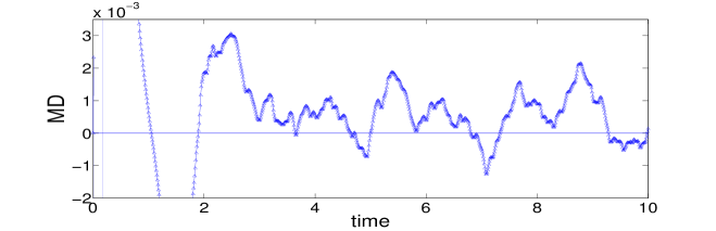
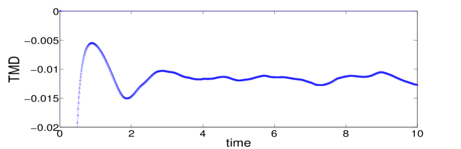
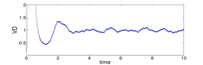
Fig. 2: $\nu=1/10000$, $\Delta t=0.01$, $m=80$, $n=60$, $\beta=8\ast 10^{-5}$.

7 Conclusions

We have shown that eddy viscosity models can be quite easily adapted to non-equilibrium turbulence and incorporate backscatter without using negative turbulent viscosities. The modified eddy viscosity model has been tested successfully for the Smagorinsky model, chosen because it is over dissipative. Some preliminary and formal calculations were given for the scaling parameter $\beta$. It may also happen that for accuracy a different fluctuation model may be needed for the viscous dissipation term and the kinetic energy term. This is an open question. Strong solutions of the new models have been proven to share the property of the true Reynolds stresses of being dissipative on time average. We have also given three methods for time discretization preserving this property, including a modular correction for an eddy viscosity code. There are many important open questions including accuracy tests, existence of weak solutions to the new models, model calibration and extension to and testing for better EV models.

References

• [1] G.K. Batchelor, The Theory of Homogeneous Turbulence, Cambridge Science Classics, 1995.
• [2] L.C. Berselli and F. Flandoli, On a stochastics approach to eddy viscosity models for turbulent flows, Adv. Math. Fluid Mech., (2010), 55-81.
• [3] L.C. Berselli, T. Iliescu and W. Layton, Mathematics of Large Eddy Simulation of Turbulent Flows, Springer, Berlin, 2006.
• [4] J. Boussinesq, Essai sur la théorie des eaux courantes, Mémoires présentés par divers savants à l’Académie des Sciences, 23 (1877): 1-680
• [5] T. Chacon-Rebollo and R. Lewandowski, Mathematical and Numerical Foundations of Turbulence Models and Applications, Springer, New-York, 2014.
• [6] P.A. Durbin and B.A. Pettersson Reif, Statistical Theory and Modeling for Turbulent Flows, Second Edition, Wiley, Chichester, 2011.
• [7] C. Egbers and G. Pfister, Physics of Rotating Fluids, Springer L.N. Physics, vol. 549, Springer, Berlin, 2000.
• [8] H. Frahnert and U. Ch. Dallman, Examination of the eddy viscosity concept regarding its physical justification, p. 255-262 in: Notes on Numerical Fluid Mechanics, vol. 77, 2002.
• [9] U. Frisch, Turbulence, Cambridge Univ. Press, Cambridge, 1995.
• [10] M.D. Gunzburger, Finite Element Methods for Viscous Incompressible Flows - A Guide to Theory, Practices, and Algorithms, Academic Press, 1989.
• [11] F. Hecht, New development in FreeFem++, J. Numer. Math. 20 (2012), 251-265.
• [12] T. Hughes, L. Mazzei and K. Jansen, Large eddy simulation and the variational multiscale method, Computing and Visualization in Science, 3 (1/2)(2000), 47-59.
• [13] T. Iliescu and W. Layton, Approximating the larger eddies in fluid motion III: The Boussinesq model for turbulent fluctuations, Analele Stinfice ale Universitatii “Al. I. Cuza” Iasi, XLIV (1998), 245-261.
• [14] N. Jiang, A higher order ensemble simulation algorithm for fluid flows, to appear: Journal of Scientific Computing, 2015, DOI: 10.1007/s10915-014-9932-z.
• [15] N. Jiang, S. Kaya Merdan and W. Layton, Analysis of model variance for ensemble based turbulence modeling, to appear in: Computational Methods in Applied Mathematics, 2015.
• [16] N. Jiang and W. Layton, An algorithm for fast calculation of flow ensembles, IJUQ, 4 (2014), 273-301.
• [17] N. Jiang and W. Layton, Numerical analysis of two ensemble eddy viscosity numerical regularizations of fluid motion, to appear in: Numerical Methods for Partial Differential Equations, 2015, DOI: 10.1002/num.21908.
• [18] W. Layton, The 1877 Boussinesq conjecture: Turbulent fluctuations are dissipative on the mean flow, 2014, available at www.mathematics.pitt.edu/research/technical-reports.
• [19] W. Layton and R. Lewandowski, Analysis of an eddy viscosity model for large eddy simulation of turbulent flows, J. Math. Fluid Mechanics, 2 (2002), 374-399.
• [20] W. Layton, L.G. Rebholz and C. Trenchea, Modular nonlinear filter stabilization of methods for higher Reynolds numbers flow, Journal of Mathematical Fluid Mechanics, 14 (2012), 325-354.
• [21] T.S. Lund and E.A. Novikov, Parametrization of subgrid-scale stress by the velocity gradient tensor, Annual Research Briefs, CTR, (1992), 27-43.
• [22] B. Mohammadi and O. Pironneau, Analysis of the k-epsilon Turbulence Model, Masson, Paris, 1994.
• [23] A.S. Monin and A.M. Yaglom, Statistical Fluid Mechanics, Mechanics of Turbulence, vol. 1, Dover publications, Mineola, 2007.
• [24] S. Pope, Turbulent Flows, Cambridge Univ. Press, Cambridge, 2000.
• [25] R.S. Rivlin, The relation between the flow of non-Newtonian fluids and turbulent Newtonian fluids, Quarterly of Appl. Math, 15 (1957), 1941-1944.
• [26] A.J.C. Saint-Venant (Barré), Note à joindre au Mémoire sur la dynamique des fluides, CRAS, 17 (1843), 1240-1243.
• [27] F.G. Schmitt, About Boussinesq’s turbulent viscosity hypothesis: historical remarks and a direct evaluation of its validity, Comptes Rendus Mécanique, 335 (2007), 617-627.
• [28] P. Sagaut, Large Eddy Simulation for Incompressible Flows, Springer, Berlin, 2001.
• [29] J. Smagorinsky, Some historical remarks on the use of nonlinear viscosities, pp. 3-36 in: Large Eddy Simulation of Complex Engineering and Geophysical Flows, B. Galperin and S.A. Orszag (editors), Cambridge U. Press, Cambridge, 1993.
• [30] V.P. Starr, Physics of Negative Viscosity Phenomena, McGraw Hill, NY, 1968.
• [31] A.W. Vreman, An eddy-viscosity subgrid-scale model for turbulent shear flow: algebraic theory and applications, Phys. Fluids, 16 (2004), 3670-3681.