Time Averaged Consensus in a Direct Coupled Distributed Coherent Quantum Observer

Abstract

This paper considers the problem of constructing a distributed direct coupling quantum observer for a closed linear quantum system. The proposed distributed observer consists of a network of quantum harmonic oscillators and it is shown that the distributed observer converges to a consensus in a time averaged sense in which each component of the observer estimates the specified output of the quantum plant. An example and simulations are included to illustrate the properties of the distributed observer.

I Introduction

In recent years, there has been significant interest in controlling networks of multi-agent systems to achieve a consensus among the agents; e.g., see [1, 2, 3, 4, 5]. In particular, some authors have looked at the problem of consensus in distributed estimation problems; e.g., see [6, 7]. Furthermore, issues of consensus have been considered in networked quantum systems; see [8, 9, 10, 11, 12]. This work is motivated by the fact that it is becoming increasingly possible for quantum control experiments to involve the networked interconnection of many quantum elements and these quantum networks will have important applications in problems such as quantum communication and quantum information processing. Also, many macroscopic systems can be regarded as consisting of a large quantum network.

In this paper, we build on the papers [13, 14] which considered the problem of constructing a direct coupling quantum observer for a given quantum system. The problem of constructing an observer for a linear quantum system has been considered in a number of recent papers; e.g, see [15, 16]. The control of linear quantum systems has been of considerable interest in recent years; e.g., see [17, 18, 19]. Such linear quantum systems commonly arise in the area of quantum optics; e.g., see [20, 21]. For such system models, an important class of control problems are coherent quantum feedback control problems; e.g., see [17, 18, 22, 23, 24, 25, 26, 27]. In these control problems, both the plant and the controller are quantum systems and the controller is designed to optimize some performance index. The coherent quantum observer problem can be regarded as a special case of the coherent quantum feedback control problem in which the objective of the observer is to estimate the system variables of the quantum plant. The papers [13, 14] considered a direct coupling coherent observer problem in which the observer is directly coupled to the plant and not coupled via a field as in previous papers. This leads the papers [13, 14] to consider a notion of time-averaged convergence for the observers.

In this paper, we extend the results of [13] to consider a direct coupled distributed quantum observer which is constructed via the direct connection of many quantum harmonic oscillators. We show that this quantum network can be constructed so that each output of the direct coupled distributed quantum observer converges to the plant output of interest in a time averaged sense. This is a form of time averaged quantum consensus for the quantum networks under consideration.

II Quantum Systems

In the distributed quantum observer problem under consideration, both the quantum plant and the distributed quantum observer are linear quantum systems; see also [17, 28, 24]. We will restrict attention to closed linear quantum systems which do not interact with an external environment. The quantum mechanical behavior of a linear quantum system is described in terms of the system observables which are self-adjoint operators on an underlying infinite dimensional complex Hilbert space $\mathfrak{H}$. The commutator of two scalar operators $x$ and $y$ on ${\mathfrak{H}}$ is defined as $[x,y]=xy-yx$. Also, for a vector of operators $x$ on ${\mathfrak{H}}$, the commutator of ${x}$ and a scalar operator $y$ on ${\mathfrak{H}}$ is the vector of operators $[{x},y]={x}y-y{x}$, and the commutator of ${x}$ and its adjoint ${x}^{\dagger}$ is the matrix of operators

$$[{x},{x}^{\dagger}]\triangleq{x}{x}^{\dagger}-({x}^{\#}{x}^{T})^{T},$$

where ${x}^{\#}\triangleq(x_{1}^{\ast}\;x_{2}^{\ast}\;\cdots\;x_{n}^{\ast})^{T}$ and ^∗ denotes the operator adjoint.

The dynamics of the closed linear quantum systems under consideration are described by non-commutative differential equations of the form

$$\dot{x}(t) = Ax(t);\quad x(0)=x_{0}$$ (1)

where $A$ is a real matrix in $\mathbb{R}^{n\times n}$, and $x(t)=[\begin{array}[]{ccc}x_{1}(t)&\ldots&x_{n}(t)\end{array}]^{T}$ is a vector of system observables; e.g., see [17]. Here $n$ is assumed to be an even number and $\frac{n}{2}$ is the number of modes in the quantum system.

The initial system variables $x(0)=x_{0}$ are assumed to satisfy the commutation relations

$$[x_{j}(0),x_{k}(0)]=2i\Theta_{jk},\ \ j,k=1,\ldots,n,$$ (2)

where $\Theta$ is a real skew-symmetric matrix with components $\Theta_{jk}$. In the case of a single quantum harmonic oscillator, we will choose $x=(x_{1},x_{2})^{T}$ where $x_{1}=q$ is the position operator, and $x_{2}=p$ is the momentum operator. The commutation relations are $[q,p]=2i$. In general, the matrix $\Theta$ is assumed to be of the form

$$\Theta={\rm diag}(J,J,\ldots,J)$$ (3)

where $J$ denotes the real skew-symmetric $2\times 2$ matrix

$$J=\left[\begin{array}[]{cc}0&1\\ -1&0\end{array}\right].$$

The system dynamics (1) are determined by the system Hamiltonian which is a which is a self-adjoint operator on the underlying Hilbert space $\mathfrak{H}$. For the linear quantum systems under consideration, the system Hamiltonian will be a quadratic form $\mathcal{H}=\frac{1}{2}x(0)^{T}Rx(0)$, where $R$ is a real symmetric matrix. Then, the corresponding matrix $A$ in (1) is given by

$$A=2\Theta R.$$ (4)

where $\Theta$ is defined as in (3). e.g., see [17]. In this case, the system variables $x(t)$ will satisfy the commutation relations at all times:

$$[x(t),x(t)^{T}]=2{\boldsymbol{i}}\Theta\ \mbox{for all }t\geq 0.$$ (5)

That is, the system will be physically realizable; e.g., see [17].

Remark 1

Note that that the Hamiltonian $\mathcal{H}$ is preserved in time for the system (1). Indeed, $\mathcal{\dot{H}}=\frac{1}{2}\dot{x}^{T}Rx+\frac{1}{2}x^{T}R\dot{x}=-x^{T}R\Theta Rx+x^{T}R\Theta Rx=0$ since $R$ is symmetric and $\Theta$ is skew-symmetric.

III Direct Coupling Distributed Coherent Quantum Observers

In our proposed direct coupling coherent quantum observer, the quantum plant is a single quantum harmonic oscillator which is a linear quantum system of the form (1) described by the non-commutative differential equation

$$\dot{x}_{p}(t) = A_{p}x_{p}(t);\quad x_{p}(0)=x_{0p};$$

$$z_{p}(t) = C_{p}x_{p}(t)$$ (6)

where $z_{p}(t)$ denotes the vector of system variables to be estimated by the observer and $A_{p}\in\mathbb{R}^{2\times 2}$, $C_{p}\in\mathbb{R}^{1\times 2}$. It is assumed that this quantum plant corresponds to a plant Hamiltonian $\mathcal{H}_{p}=\frac{1}{2}x_{p}(0)^{T}R_{p}x_{p}(0)$. Here $x_{p}=\left[\begin{array}[]{l}q_{p}\\ p_{p}\end{array}\right]$ where $q_{p}$ is the plant position operator and $p_{p}$ is the plant momentum operator.

We now describe the linear quantum system of the form (1) which will correspond to the distributed quantum observer; see also [17, 28, 24]. This system is described by a non-commutative differential equation of the form

$$\dot{x}_{o}(t) = A_{o}x_{o}(t);\quad x_{o}(0)=x_{0o};$$

$$z_{o}(t) = C_{o}x_{o}(t)$$ (7)

where the observer output $z_{o}(t)$ is the distributed observer estimate vector and $A_{p}\in\mathbb{R}^{n_{o}\times n_{o}}$, $C_{o}\in\mathbb{R}^{\frac{n_{o}}{2}\times n_{o}}$. Also, $x_{o}(t)$ is a vector of self-adjoint non-commutative system variables; e.g., see [17]. We assume the distributed observer order $n_{o}$ is an even number with $N=\frac{n_{o}}{2}$ being the number of elements in the distributed quantum observer. We also assume that the plant variables commute with the observer variables. The system dynamics (7) are determined by the observer system Hamiltonian which is a which is a self-adjoint operator on the underlying Hilbert space for the observer. For the distributed quantum observer under consideration, this Hamiltonian is given by a quadratic form: $\mathcal{H}_{o}=\frac{1}{2}x_{o}(0)^{T}R_{o}x_{o}(0)$, where $R_{o}$ is a real symmetric matrix. Then, the corresponding matrix $A_{o}$ in (7) is given by

$$A_{o}=2\Theta R_{o}$$ (8)

where $\Theta$ is defined as in (3). Furthermore, we will assume that the distributed quantum observer has a chain structure and is coupled to the quantum plant as shown in Figure 1.

Figure 1: Distributed Quantum Observer.

This corresponds to an observer Hamiltonian of the form

$$\mathcal{H}_{o} = \frac{1}{2}x_{o}(0)^{T}R_{o}x_{o}(0)$$

$$= \frac{1}{2}\sum_{i=1}^{N}x_{oi}(0)^{T}R_{oi}x_{oi}(0)$$

$$+\sum_{i=1}^{N-1}x_{oi}(0)^{T}R_{c(i+1)}x_{o(i+1)}(0)$$

where the vector of observer system variables $x_{o}$ is partitioned according to each element of the distributed quantum observer as follows

$$x_{o}=\left[\begin{array}[]{l}x_{o1}\\ x_{o2}\\ \vdots\\ x_{oN}\end{array}\right].$$

We assume that the variables for each element of the distributed quantum observer commute with the variables of all other elements of the distributed quantum observer; i.e.,

$$[x_{oi},x_{oj}^{T}]=0~{}~{}\forall~{}~{}i\neq j.$$

Here, $x_{oi}=\left[\begin{array}[]{l}q_{oi}\\ p_{oi}\end{array}\right]$ for $i=1,2,\ldots,N$ where $q_{oi}$ is the position operator for the $i$th observer element and $p_{oi}$ is the momentum operator for the $i$th observer element.

In addition, we define a coupling Hamiltonian which defines the coupling between the quantum plant and the first element of the distributed quantum observer:

$$\mathcal{H}_{c}=x_{p}(0)^{T}R_{c1}x_{o1}(0).$$

Furthermore, we write

$$z_{o}=\left[\begin{array}[]{l}z_{o1}\\ z_{o2}\\ \vdots\\ z_{oN}\end{array}\right]$$

where

$$z_{oi}=C_{oi}x_{oi}\mbox{ for }i=1,2,\ldots,N.$$

Note that $R_{oi}\in\mathbb{R}^{2\times 2}$, $R_{ci}\in\mathbb{R}^{2\times 2}$, $C_{oi}\in\mathbb{R}^{1\times 2}$, and each matrix $R_{oi}$ is symmetric for $i=1,2,\ldots,N$.

The augmented quantum linear system consisting of the quantum plant and the distributed quantum observer is then a quantum system of the form (1) described by the total Hamiltonian

$$\mathcal{H}_{a} = \mathcal{H}_{p}+\mathcal{H}_{c}+\mathcal{H}_{o}$$ (9)

$$= \frac{1}{2}x_{a}(0)^{T}R_{a}x_{a}(0)$$

where

$$x_{a}=\left[\begin{array}[]{l}x_{p}\\ x_{o1}\\ x_{o2}\\ \vdots\\ x_{oN}\end{array}\right],~{}~{}R_{a}=\left[\begin{array}[]{lllll}R_{p}&R_{c1}&&&\\ R_{c1}^{T}&R_{o1}&R_{c2}&&0\\ &R_{c2}^{T}&R_{o2}&\ddots&\\ 0&&\ddots&\ddots&R_{cN}\\ &&&R_{cN}^{T}&R_{oN}\end{array}\right].$$ (10)

Then, using (4), it follows that the augmented quantum linear system is described by the equations

$$\left[\begin{array}[]{l}\dot{x}_{p}(t)\\ \dot{x}_{o1}(t)\\ \dot{x}_{o2}(t)\\ \vdots\\ \dot{x}_{oN}(t)\end{array}\right] = A_{a}\left[\begin{array}[]{l}x_{p}(t)\\ x_{o1}(t)\\ x_{o2}(t)\\ \vdots\\ x_{oN}(t)\end{array}\right];$$ (21)

$$z_{p}(t) = C_{p}x_{p}(t);$$

$$z_{o}(t) = C_{o}x_{o}(t)$$ (22)

where $A_{a}=2\Theta R_{a}$ and

$$C_{o}=\left[\begin{array}[]{llll}C_{o1}&&&\\ &C_{o2}&0&\\ &0&\ddots&\\ &&&C_{oN}\end{array}\right].$$

We now formally define the notion of a direct coupled linear quantum observer.

Definition 1

The matrices $R_{o1}$, $R_{o2}$, $\ldots$, $R_{oN}$, $R_{c1}$, $R_{c2}$, $\ldots$, $R_{cN}$, $C_{o1}$, $C_{o2}$, $\ldots$, $C_{oN}$ define a distributed linear quantum observer achieving time-averaged consensus convergence for the quantum linear plant (6) if the corresponding augmented linear quantum system (22) is such that

$$\lim_{T\rightarrow\infty}\frac{1}{T}\int_{0}^{T}(\left[\begin{array}[]{l}1\\ 1\\ \vdots\\ 1\end{array}\right]z_{p}(t)-z_{o}(t))dt=0.$$ (23)

Remark 2

Note that the above definition requires that the time average of each observer element output $z_{oi}(t)$ converges to the time average of the plant output $z_{p}(t)$. That is, an averaged consensus is reached by the observer element outputs.

IV Constructing a Direct Coupling Distributed Coherent Quantum Observer

We now describe the construction of a distributed linear quantum observer. In this section, we assume that $A_{p}=0$ in (6). This corresponds to $R_{p}=0$ in the plant Hamiltonian. It follows from (6) that the plant system variables $x_{p}(t)$ will remain fixed if the plant is not coupled to the observer. However, when the plant is coupled to the quantum observer this will no longer be the case. We will show that if the distributed quantum observer is suitably designed, the plant quantity to be estimated $z_{p}(t)$ will remain fixed and the condition (23) will be satisfied.

We assume that the matrices $R_{ci}$, $R_{oi}$ are of the form

$$R_{ci}=\alpha_{i}\beta_{i}^{T},~{}~{}R_{oi}=\omega_{i}I$$ (24)

where $\alpha_{i}\in\mathbb{R}^{2}$, $\beta_{i}\in\mathbb{R}^{2}$ and $\omega_{i}>0$ for $i=1,2,\ldots,N$. Also, we assume that $\alpha_{1}=C_{p}^{T}$.

We will show that these assumptions imply that the quantity $z_{p}(t)=C_{p}x_{p}(t)$ will be constant for the augmented quantum system (22). Indeed, it follows from (22), (10), (3) that

$$\dot{x}_{p}(t)=2JR_{c1}x_{o1}(t)=2J\alpha_{1}\beta_{1}^{T}x_{o1}(t).$$

Hence,

$$\dot{z}_{p}(t)=2C_{p}J\alpha_{1}\beta_{1}^{T}x_{o1}(t)=2\alpha_{1}^{T}J\alpha_{1}\beta_{1}^{T}x_{o1}(t)=0$$

since $J$ skew-symmetric implies $\alpha_{1}^{T}J\alpha_{1}=0$. Therefore,

$$z_{p}(t)=z_{p}(0)=z_{p}$$ (25)

for all $t\geq 0$.

It now follows from (22) that we can write

$$\left[\begin{array}[]{l}\dot{x}_{o1}(t)\\ \dot{x}_{o2}(t)\\ \vdots\\ \dot{x}_{oN}(t)\end{array}\right] = A_{o}\left[\begin{array}[]{l}x_{o1}(t)\\ x_{o2}(t)\\ \vdots\\ x_{oN}(t)\end{array}\right]+2\left[\begin{array}[]{l}J\beta_{1}\alpha_{1}^{T}\\ 0\\ \vdots\\ 0\end{array}\right]x_{p}(t);$$

$$= A_{o}\left[\begin{array}[]{l}x_{o1}(t)\\ x_{o2}(t)\\ \vdots\\ x_{oN}(t)\end{array}\right]+B_{o}z_{p}$$

where

$$A_{o}=2\left[\begin{array}[]{lllll}\omega_{1}J&J\alpha_{2}\beta_{2}^{T}&&&\\ J\beta_{2}\alpha_{2}^{T}&\omega_{2}J&J\alpha_{3}\beta_{3}^{T}&&0\\ &J\beta_{3}\alpha_{3}^{T}&\omega_{3}J&\ddots&\\ 0&&\ddots&\ddots&J\alpha_{N}\beta_{N}^{T}\\ &&&J\beta_{N}\alpha_{N}^{T}&\omega_{N}J\end{array}\right]$$

and

$$B_{o}=\left[\begin{array}[]{l}2J\beta_{1}\\ 0\\ \vdots\\ 0\end{array}\right].$$

To construct a suitable distributed quantum observer, we will further assume that

$$\alpha_{i}=\alpha=C_{p}^{T},~{}~{}\beta_{i}=-\mu_{i}\alpha\mbox{ and }C_{oi}=C_{p}=\alpha^{T}$$ (28)

for all $i=1,2,\ldots,N$ where each $\mu_{i}>0$. In order to construct suitable values for the quantities $\mu_{i}$ and $\omega_{i}$, we require that

$$A_{o}\left[\begin{array}[]{l}\alpha\\ \alpha\\ \vdots\\ \alpha\end{array}\right]+B_{o}\|\alpha\|^{2}=0.$$ (29)

This will ensure that the quantity

$$\tilde{x}_{o}=x_{o}-\frac{1}{\|\alpha\|^{2}}\left[\begin{array}[]{l}\alpha\\ \alpha\\ \vdots\\ \alpha\end{array}\right]z_{p}$$ (30)

will satisfy the non-commutative differential equation

$$\dot{\tilde{x}}_{o}=A_{o}\tilde{x}_{o}.$$ (31)

This, combined with the fact that

$$C_{o}\frac{1}{\|\alpha\|^{2}}\left[\begin{array}[]{l}\alpha\\ \alpha\\ \vdots\\ \alpha\end{array}\right]z_{p}$$ (36)

$$= \frac{1}{\|\alpha\|^{2}}\left[\begin{array}[]{llll}\alpha^{T}&&&\\ &\alpha^{T}&0&\\ &0&\ddots&\\ &&&\alpha^{T}\end{array}\right]\left[\begin{array}[]{l}\alpha\\ \alpha\\ \vdots\\ \alpha\end{array}\right]z_{p}$$ (45)

$$= \left[\begin{array}[]{l}1\\ 1\\ \vdots\\ 1\end{array}\right]z_{p}$$ (50)

will be used in establishing the condition (23) for the distributed quantum observer.

Now we require

$$A_{o}\left[\begin{array}[]{l}\alpha\\ \alpha\\ \vdots\\ \alpha\end{array}\right]+B_{o}\|\alpha\|^{2}$$

$$= 2\left[\begin{array}[]{c}\omega_{1}J\alpha-\mu_{2}J\alpha\|\alpha\|^{2}-\mu_{1}J\alpha\|\alpha\|^{2}\\ -\mu_{2}J\alpha\|\alpha\|^{2}+\omega_{2}J\alpha-\mu_{3}J\alpha\|\alpha\|^{2}\\ -\mu_{3}J\alpha\|\alpha\|^{2}+\omega_{3}J\alpha-\mu_{4}J\alpha\|\alpha\|^{2}\\ \vdots\\ -\mu_{N}J\alpha\|\alpha\|^{2}+\omega_{N}J\alpha\end{array}\right]$$

$$= 0.$$

This will be satisfied if and only if

$$\left[\begin{array}[]{c}\omega_{1}-\mu_{2}\|\alpha\|^{2}-\mu_{1}\|\alpha\|^{2}\\ -\mu_{2}\|\alpha\|^{2}+\omega_{2}-\mu_{3}\|\alpha\|^{2}\\ -\mu_{3}\|\alpha\|^{2}+\omega_{3}-\mu_{4}\|\alpha\|^{2}\\ \vdots\\ -\mu_{N}\|\alpha\|^{2}+\omega_{N}\end{array}\right]=0.$$

That is, we require that

$$\omega_{i}=(\mu_{i}+\mu_{i+1})\|\alpha\|^{2}$$ (53)

for $i=1,2,\ldots,N-1$ and

$$\omega_{N}=\mu_{N}\|\alpha\|^{2}.$$ (54)

To show that the above candidate distributed quantum observer leads to the satisfaction of the condition (23), we first note that $\tilde{x}_{o}$ defined in (30) will satisfy (31). If we can show that

$$\lim_{T\rightarrow\infty}\frac{1}{T}\int_{0}^{T}\tilde{x}_{o}(t)dt=0$$ (55)

then it will follow from (36) and (29) that (23) is satisfied. In order to establish (55), we first note that we can write

$$A_{o}=2\Theta R_{o}$$

where

$$R_{o}=$$

$$\left[\begin{array}[]{rrrrr}\omega_{1}I&-\mu_{2}\alpha\alpha^{T}&&&\\ -\mu_{2}\alpha\alpha^{T}&\omega_{2}I&-\mu_{3}\alpha\alpha^{T}&&0\\ &-\mu_{3}\alpha\alpha^{T}&\omega_{3}I&\ddots&\\ 0&&\ddots&\ddots&-\mu_{N}\alpha\alpha^{T}\\ &&&-\mu_{N}\alpha\alpha^{T}&\omega_{N}I\end{array}\right].$$

We will now show that the symmetric matrix $R_{o}$ is positive-definite.

Lemma 1

The matrix $R_{o}$ is positive definite.

Proof:

In order to establish this lemma, let

$$x_{o}=\left[\begin{array}[]{l}x_{o1}\\ x_{o2}\\ \vdots\\ x_{oN}\end{array}\right]$$

be a non-zero real vector. Then

$$x_{o}^{T}R_{o}x_{o} = \omega_{1}\|x_{o1}\|^{2}-2\mu_{2}x_{o1}^{T}\alpha x_{o2}^{T}\alpha+\omega_{2}\|x_{o2}\|^{2}$$

$$-2\mu_{3}x_{o2}^{T}\alpha x_{o3}^{T}\alpha+\omega_{3}\|x_{o3}\|^{2}$$

$$\vdots$$

$$-2\mu_{N}x_{oN-1}^{T}\alpha x_{oN}^{T}\alpha+\omega_{N}\|x_{oN}\|^{2}$$

$$\geq \omega_{1}\|x_{o1}\|^{2}-2\mu_{2}\|x_{o1}\|\|x_{o2}\|\|\alpha\|^{2}+\omega_{2}\|x_{o2}\|^{2}$$

$$-2\mu_{3}\|x_{o2}|\|x_{o3}\|\|\alpha\|^{2}+\omega_{3}\|x_{o3}\|^{2}$$

$$\vdots$$

$$-2\mu_{N}\|x_{oN-1}\|\|x_{oN}\|\|\alpha\|^{2}+\omega_{N}\|x_{oN}\|^{2}$$

using the Cauchy-Schwarz inequality. Hence,

$$x_{o}^{T}R_{o}x_{o} \geq \omega_{1}\|x_{o1}\|^{2}-2\tilde{\mu}_{2}\|x_{o1}\|\|x_{o2}\|+\omega_{2}\|x_{o2}\|^{2}$$ (57)

$$-2\tilde{\mu}_{3}\|x_{o2}|\|x_{o3}\|+\omega_{3}\|x_{o3}\|^{2}$$

$$\vdots$$

$$-2\tilde{\mu}_{N}\|x_{oN-1}\|\|x_{oN}\|+\omega_{N}\|x_{oN}\|^{2}$$

where

$$\tilde{\mu}_{i}=\mu_{i}\|\alpha\|^{2}$$ (58)

for $i=1,2,\ldots,N$. Thus, (57) implies

$$x_{o}^{T}R_{o}x_{o}\geq\check{x}_{o}^{T}\tilde{R}_{o}\check{x}_{o}$$

where

$$\check{x}_{o}=\left[\begin{array}[]{c}\|x_{o1}\|\\ \|x_{o2}\|\\ \vdots\\ \|x_{oN}\|\end{array}\right]$$

and

$$\tilde{R}_{o}=\left[\begin{array}[]{rrrrr}\omega_{1}&-\tilde{\mu}_{2}&&&\\ -\tilde{\mu}_{2}&\omega_{2}&-\tilde{\mu}_{3}&&0\\ &-\tilde{\mu}_{3}&\omega_{3}&\ddots&\\ 0&&\ddots&\ddots&-\tilde{\mu}_{N}\\ &&&-\tilde{\mu}_{N}&\omega_{N}\end{array}\right].$$

Now the vector $\check{x}_{o}$ will be non-zero if and only if the vector $x_{o}$ is non-zero. Hence, the matrix $R_{o}$ will be positive-definite if we can show that the matrix $\tilde{R}_{o}$ is positive-definite. In order to establish this fact, we first note that (53), (54) and (58) imply that

$$\omega_{i}=\tilde{\mu}_{i}+\tilde{\mu}_{i+1}$$

for $i=1,2,\ldots,N-1$ and

$$\omega_{N}=\tilde{\mu}_{N}.$$

Hence, we can write

$$\tilde{R}_{o} = \left[\begin{array}[]{rrrrr}\tilde{\mu}_{1}+\tilde{\mu}_{2}&-\tilde{\mu}_{2}&&&\\ -\tilde{\mu}_{2}&\tilde{\mu}_{2}+\tilde{\mu}_{3}&-\tilde{\mu}_{3}&&0\\ &-\tilde{\mu}_{3}&\tilde{\mu}_{3}+\tilde{\mu}_{4}&\ddots&\\ 0&&\ddots&\ddots&-\tilde{\mu}_{N}\\ &&&-\tilde{\mu}_{N}&\tilde{\mu}_{N}\end{array}\right]$$

$$= \tilde{R}_{o1}+\tilde{R}_{o2}$$

where

$$\tilde{R}_{o1}=\left[\begin{array}[]{rrrr}\tilde{\mu}_{1}&0&\ldots&0\\ 0&0&\ldots&0\\ \vdots&&&\vdots\\ 0&0&\ldots&0\end{array}\right]\geq 0$$

and

$$\tilde{R}_{o2}=\left[\begin{array}[]{rrrrr}\tilde{\mu}_{2}&-\tilde{\mu}_{2}&&&\\ -\tilde{\mu}_{2}&\tilde{\mu}_{2}+\tilde{\mu}_{3}&-\tilde{\mu}_{3}&&0\\ &-\tilde{\mu}_{3}&\tilde{\mu}_{3}+\tilde{\mu}_{4}&\ddots&\\ 0&&\ddots&\ddots&-\tilde{\mu}_{N}\\ &&&-\tilde{\mu}_{N}&\tilde{\mu}_{N}\end{array}\right].$$

Now the matrix $\tilde{R}_{o2}$ is the Laplacian matrix for the weighted graph shown in Figure 2.

Figure 2: Underlying weighted graph for distributed quantum observer. This corresponds to the observer structure shown in Figure 1.

Since this graph is a connected graph, it follows that the matrix $\tilde{R}_{o2}$ is positive-semidefinite with null space equal to

$$\mathcal{N}(\tilde{R}_{o2})=\mbox{span}\{\left[\begin{array}[]{l}1\\ 1\\ \vdots\\ 1\end{array}\right]\}.$$

The fact that $\tilde{R}_{o1}\geq 0$ and $\tilde{R}_{o2}\geq 0$ implies that $\tilde{R}_{o}\geq 0$. In order to show that $\tilde{R}_{o}>0$, suppose that $x$ is a non-zero vector in $\mathcal{N}(\tilde{R}_{o})$. It follows that

$$x^{T}\tilde{R}_{o}x=x^{T}\tilde{R}_{o1}x+x^{T}\tilde{R}_{o2}x=0.$$

Since $\tilde{R}_{o1}\geq 0$ and $\tilde{R}_{o2}\geq 0$, $x$ must be contained in the null space of $\tilde{R}_{o1}$ and the null space of $\tilde{R}_{o2}$. Therefore $x$ must be of the form

$$x=\gamma\left[\begin{array}[]{l}1\\ 1\\ \vdots\\ 1\end{array}\right]$$

where $\gamma\neq 0$. However, then

$$x^{T}\tilde{R}_{o1}x=\gamma^{2}\tilde{\mu}_{1}\neq 0$$

and hence $x$ cannot be in the null space of $\tilde{R}_{o1}$. Thus, we can conclude that the matrix $\tilde{R}_{o}$ is positive definite and hence, the matrix $R_{o}$ is positive definite. This completes the proof of the lemma. ∎

We now verify that the condition (23) is satisfied for the distributed quantum observer under consideration. We recall from Remark 1 that the quantity $\frac{1}{2}\tilde{x}_{o}(t)^{T}R_{o}\tilde{x}_{o}(t)$ remains constant in time for the linear system:

$$\dot{\tilde{x}}_{o}=A_{o}\tilde{x}_{o}=2\Theta R_{o}\tilde{x}_{o}.$$

That is

$$\frac{1}{2}\tilde{x}_{o}(t)^{T}R_{o}\tilde{x}_{o}(t)=\frac{1}{2}\tilde{x}_{o}(0)^{T}R_{o}\tilde{x}_{o}(0)\quad\forall t\geq 0.$$ (60)

However, $\tilde{x}_{o}(t)=e^{2\Theta R_{o}t}\tilde{x}_{o}(0)$ and $R_{o}>0$. Therefore, it follows from (60) that

$$\sqrt{\lambda_{min}(R_{o})}\|e^{2\Theta R_{o}t}\tilde{x}_{o}(0)\|\leq\sqrt{\lambda_{max}(R_{o})}\|\tilde{x}_{o}(0)\|$$

for all $\tilde{x}_{o}(0)$ and $t\geq 0$. Hence,

$$\|e^{2\Theta R_{o}t}\|\leq\sqrt{\frac{\lambda_{max}(R_{o})}{\lambda_{min}(R_{o})}}$$ (61)

for all $t\geq 0$.

Now since $\Theta$ and $R_{o}$ are non-singular,

$$\int_{0}^{T}e^{2\Theta R_{o}t}dt=\frac{1}{2}e^{2\Theta R_{o}T}R_{o}^{-1}\Theta^{-1}-\frac{1}{2}R_{o}^{-1}\Theta^{-1}$$

and therefore, it follows from (61) that

$$\frac{1}{T}\|\int_{0}^{T}e^{2\Theta R_{o}t}dt\|$$

$$= \frac{1}{T}\|\frac{1}{2}e^{2\Theta R_{o}T}R_{o}^{-1}\Theta^{-1}-\frac{1}{2}R_{o}^{-1}\Theta^{-1}\|$$

$$\leq \frac{1}{2T}\|e^{2\Theta R_{o}T}\|\|R_{o}^{-1}\Theta^{-1}\|$$

$$+\frac{1}{2T}\|R_{o}^{-1}\Theta^{-1}\|$$

$$\leq \frac{1}{2T}\sqrt{\frac{\lambda_{max}(R_{o})}{\lambda_{min}(R_{o})}}\|R_{o}^{-1}\Theta^{-1}\|$$

$$+\frac{1}{2T}\|R_{o}^{-1}\Theta^{-1}\|$$

$$\rightarrow 0$$

as $T\rightarrow\infty$. Hence,

$$\lim_{T\rightarrow\infty}\frac{1}{T}\|\int_{0}^{T}\tilde{x}_{o}(t)dt\|$$

$$= \lim_{T\rightarrow\infty}\frac{1}{T}\|\int_{0}^{T}e^{2\Theta R_{o}t}\tilde{x}_{o}(0)dt\|$$

$$\leq \lim_{T\rightarrow\infty}\frac{1}{T}\|\int_{0}^{T}e^{2\Theta R_{o}t}dt\|\|\tilde{x}_{o}(0)\|$$

$$= 0.$$

This implies

$$\lim_{T\rightarrow\infty}\frac{1}{T}\int_{0}^{T}\tilde{x}_{o}(t)dt=0$$

and hence, it follows from (30) and (36) that

$$\lim_{T\rightarrow\infty}\frac{1}{T}\int_{0}^{T}z_{o}(t)dt=\left[\begin{array}[]{l}1\\ 1\\ \vdots\\ 1\end{array}\right]z_{p}.$$

Also, (25) implies

$$\lim_{T\rightarrow\infty}\frac{1}{T}\int_{0}^{T}z_{p}(t)dt=\left[\begin{array}[]{l}1\\ 1\\ \vdots\\ 1\end{array}\right]z_{p}.$$

Therefore, condition (23) is satisfied. Thus, we have established the following theorem.

Theorem 1

Consider a quantum plant of the form (6) where $A_{p}=0$. Then the matrices $R_{oi}>0$, $R_{ci}$, $C_{oi}$, $i=1,2,...N$ given as in (24), (28), (53), (54) will define a distributed direct coupled quantum observer achieving time-averaged consensus convergence for this quantum plant.

Remark 3

The distributed quantum observer constructed above is determined by choice of the positive parameters $\tilde{\mu}_{1},\tilde{\mu}_{2},\ldots,\tilde{\mu}_{N}$. A number of possible choices for these parameters could be considered. One choice is to choose all of these parameters to be the same as $\tilde{\mu}_{i}=\omega_{0}$ for $i=1,2,\ldots,N$ where $\omega_{0}>0$ is a frequency parameter. This choice will mean that all of the oscillator frequencies in the distributed observer, except for the last one, will be the same, $\omega_{i}=2\omega_{0}$ for $i=1,2,\ldots,N-1$ and $\omega_{N}=\omega_{0}$. In order to have distinct oscillator frequencies in the distributed observer, we can choose $\tilde{\mu}_{i}=i\omega_{0}$ for $i=1,2,\ldots,N$. This would yield $\omega_{i}=(2i+1)\omega_{0}$ for $i=1,2,\ldots,N-1$ and $\omega_{N}=N\omega_{0}$. This means that only odd harmonics of the fundamental frequency $\omega_{0}$ are used. Alternatively, in order to obtain both odd and even harmonics of the fundamental frequency $\omega_{0}$, for the case in which $N$ is even, we can choose

$$\tilde{\mu}_{2i}=\tilde{\mu}_{2i-1}=\omega_{0}(\frac{N}{2}+1-i)>0$$ (62)

for $i=1,2,\ldots,\frac{N}{2}$. This leads to

$$\omega_{i}=\omega_{0}(N+1-i)$$ (63)

for $i=1,2,\ldots,N$. A similar choice can be derived for the case in which $N$ is odd.

Another possible approach is to choose the parameters $\tilde{\mu}_{1},\tilde{\mu}_{2},\ldots,\tilde{\mu}_{N}$ randomly with a uniform distribution on $[0,\omega_{0}N]$.

Remark 4

The proof of the above theorem relies an a graph theoretic argument used in the proof of Lemma 1. This motivates a possible extension of the result in which the distributed direct coupled observer corresponding to the weighted graph in Figure 2 is replaced by a more general distributed direct coupled observer corresponding to a more general weighted graph.

V Illustrative Example

We now present some numerical simulations to illustrate the direct coupled distributed quantum observer described in the previous section. We choose the quantum plant to have $A_{p}=0$ and $C_{p}=[1~{}~{}0]$. That is, the variable to be estimated by the quantum observer is the position operator of the quantum plant; i.e., $z_{p}(t)=q_{p}(t)$ where $x_{p}(t)=\left[\begin{array}[]{l}q_{p}(t)\\ p_{p}(t)\end{array}\right]$. For the distributed quantum observer, we choose $N=5$ so that the distributed quantum observer has five elements. Also, as discussed in Remark 3, we choose the parameters $\tilde{\mu}_{1},\tilde{\mu}_{2},\ldots,\tilde{\mu}_{N}$ so that $\tilde{\mu}_{i}=i\omega_{0}$ for $i=1,2,\ldots,N$ where $\omega_{0}=1$. Then the corresponding distributed quantum observer is defined by equations (24), (28), (53), (54).

The augmented plant-observer system is described by the equations (22), (10). Then, we can write

$$x_{a}(t)=\Phi(t)x_{a}(0)$$

where

$$\Phi(t)=e^{A_{a}t}.$$

Thus, the plant variable to be estimated $z_{p}(t)$ is given by

$$z_{p}(t) = e_{1}C_{a}\Phi(t)x_{a}(0)$$

$$= \sum_{i=1}^{2N+2}e_{1}C_{a}\Phi_{i}(t)x_{ai}(0)$$

where

$$C_{a}=\left[\begin{array}[]{ll}C_{p}&0\\ 0&C_{o}\end{array}\right],$$

$e_{1}$ is the first unit vector in the standard basis for $\mathbb{R}^{N+1}$, $\Phi_{i}(t)$ is the $i$th column of the matrix $\Phi(t)$ and $x_{ai}(0)$ is the $i$th component of the vector $x_{a}(0)$. We plot each of the quantities $e_{1}C_{a}\Phi_{1}(t),e_{1}C_{a}\Phi_{2}(t),\ldots,e_{1}C_{a}\Phi_{2N+2}(t)$ in Figure 3(a).

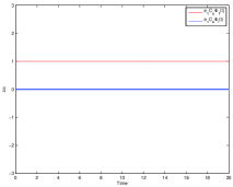
(a)

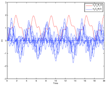
(b)

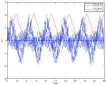
(c)

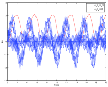
(d)

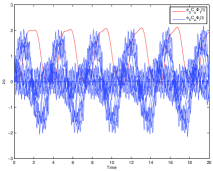
(e)

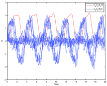
(f)

Figure 3: Coefficients defining (a) $z_{p}(t)$, (b) $z_{o1}(t)$, (c) $z_{o2}(t)$, (d) $z_{o3}(t)$, (e) $z_{o4}(t)$, and (f) $z_{o5}(t)$.

From this figure, we can see that $e_{1}C_{a}\Phi_{1}(t)\equiv 1$ and $e_{1}C_{a}\Phi_{2}(t)\equiv 0$, $e_{1}C_{a}\Phi_{2}(t)\equiv 0$, $\ldots$, $e_{1}C_{a}\Phi_{2N+2}(t)\equiv 0$, and $z_{p}(t)$ will remain constant at $z_{p}(0)$ for all $t\geq 0$.

We now consider the output variables of the distributed quantum observer $z_{oi}(t)$ for $i=1,2,\ldots,N$ which are given by

$$z_{oi}(t)=\sum_{j=1}^{2N+2}e_{i+1}C_{a}\Phi_{j}(t)x_{aj}(0)$$

where $e_{i+1}$ is the $(i+1)$th unit vector in the standard basis for $\mathbb{R}^{N+1}$. We plot each of the quantities $e_{i+1}C_{a}\Phi_{1}(t),e_{i+1}C_{a}\Phi_{2}(t),\ldots,e_{i+1}C_{a}\Phi_{2N+2}(t)$ in Figures 3(b) - 3(f).

Also, we can consider the spatial average obtained by averaging over each of the distributed observer outputs:

$$z_{os}(t)=\frac{1}{N}\sum_{i=1}^{N}z_{oi}(t)=\frac{1}{N}\sum_{i=1}^{N}\sum_{j=1}^{2N+2}e_{i+1}C_{a}\Phi_{j}(t)x_{aj}(0).$$

Then we plot each of the quantities $\frac{1}{N}\sum_{i=1}^{N}e_{i+1}C_{a}\Phi_{1}(t)$, $\frac{1}{N}\sum_{i=1}^{N}e_{i+1}C_{a}\Phi_{2}(t)$, $\ldots$ , $\frac{1}{N}\sum_{i=1}^{N}e_{i+1}C_{a}\Phi_{2N+2}(t)$ in Figure 4.

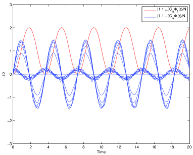
Figure 4: Coefficients defining $z_{os}(t)$.

To illustrate the time average convergence property of the quantum observer (23), we now plot the quantities $\frac{1}{T}\int_{0}^{T}e_{i+1}C_{a}\Phi_{1}(t)dt$, $\frac{1}{T}\int_{0}^{T}e_{i+1}C_{a}\Phi_{2}(t)dt$, $\ldots$, $\frac{1}{T}\int_{0}^{T}e_{i+1}C_{a}\Phi_{2N+2}(t)dt$ for $i=1,2,\ldots,N$ in Figures 5(a)-5(e). These quantities determine the averaged value of the $i$th observer output

$$z_{oi}^{ave}(T)=\frac{1}{T}\int_{0}^{T}\sum_{j=1}^{2N+2}e_{i+1}C_{a}\Phi_{j}(t)x_{aj}(0)dt$$

for $i=1,2,\ldots,N$.

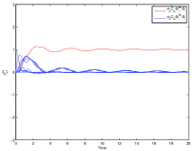
(a)

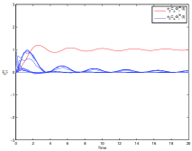
(b)

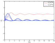
(c)

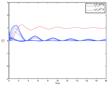
(d)

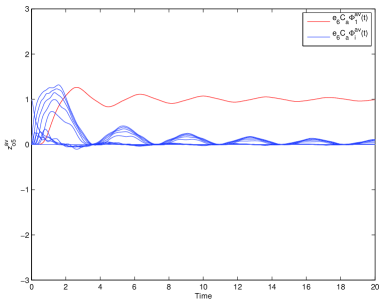
(e)

Figure 5: Coefficients defining the time average of (a) $z_{o1}(t)$, (b) $z_{o2}(t)$, (c) $z_{o3}(t)$, (d) $z_{o4}(t)$, and (e) $z_{o5}(t)$.

From these figures, we can see that for each $i=1,2,\ldots,N$, the time average of $z_{oi}(t)$ converges to $z_{p}(0)$ as $t\rightarrow\infty$. That is, the distributed quantum observer reaches a time averaged consensus corresponding to the output of the quantum plant which is to be estimated.

VI Conclusions

In this paper we have considered the construction of a distributed direct coupling observer for a closed quantum linear system in order to achieve a time averaged consensus convergence. We have also presented an illustrative example along with simulations to investigate the consensus behavior of the distributed direct coupling observer.

References

[1]
F. L. Lewis, H. Zhang, K. Hengser-Movric, and A. Das, Cooperative Control
of Multi-Agent Systems. London:
Springer, 2014.
[2]
G. Shi and K. H. Johansson, “Robust consusus for continuous-time multi-agent
dynamics,” SIAM Journal on Control and Optimization, vol. 51, no. 5,
pp. 3673–3691, 2013.
[3]
M. Mesbahi and M. Egerstedt, Graph Theoretic Methods in Multiagent
Networks. Princeton University Press,
2010.
[4]
L. Xiao and S. Boyd, “Fast linear iterations for distributed averaging,”
Systems and Control Letters, vol. 53, pp. 65–78, 2005.
[5]
A. Jadbabaie, J. Lin, and A. Morse, “Coordination of groups of mobile
autonomous agents using nearest neighbor rules,” IEEE Transactions on
Automatic Control, vol. 48, no. 6, pp. 988 – 1001, june 2003.
[6]
R. Olfati-Saber, “Distributed Kalman filter with embedded consensus
filters,” in Proceedings of the 44th IEEE Conference on Decision and
Control and the European Control Conference, Seville, Spain, December 2005,
pp. 8179–8184.
[7]
——, “Kalman-consensus filter: optimality, stability, and performance,” in
Proceedings of the 48th IEEE Conference on Decision and Control and
28th Chinese Control Conference, Shanghai, China, December 2009, pp.
7036–7042.
[8]
R. Sepulchre, A. Sarlette, and P. Rouchon, “Consensus in non-commutative
spaces,” in Proceedings of the 49th IEEE Conference on Decision and
Control, Atlanta, USA, December 2010, pp. 6596–6601.
[9]
L. Mazzarella, A. Sarlette, and F. Ticozzi, “Consensus for quantum networks:
from symmetry to gossip iterations,” IEEE Transactions on Automatic
Control, 2013, in press, preliminary version arXiv 1304.4077.
[10]
L. Mazzarella, F. Ticozzi, and A. Sarlette, “From consensus to robust
randomized algorithms: A symmetrization approach,” 2013, quant-ph, arXiv
1311.3364.
[11]
F. Ticozzi, L. Mazzarella, and A. Sarlette, “Symmetrization for quantum
networks: a continuous-time approach,” in Proceedings of the 21st
International Symposium on Mathematical Theory of Networks and Systems
(MTNS), Groningen, The Netherlands, July 2014, avaiable quant-ph, arXiv
1403.3582.
[12]
G. Shi, D. Dong, I. R. Petersen, and K. H. Johansson, “Consensus of quantum
networks with continuous-time markovian dynamics,” in Proceedings of
the 11th World Congress on Intelligent Control and Automation, 2014.
[13]
I. R. Petersen, “A direct coupling coherent quantum observer,” in
Proceedings of the 2014 IEEE Multi-conference on Systems and Control,
Antibes, France, October 2014, to appear, accepted 15 July 2014, also
available arXiv 1408.0399.
[14]
——, “A direct coupling coherent quantum observer for a single qubit finite
level quantum system,” in Proceedings of 2014 Australian Control
Conference, Canberra, Australia, November 2014, to appear, accepted 14 Aug
2014. Also arXiv 1409.2594.
[15]
Z. Miao and M. R. James, “Quantum observer for linear quantum stochastic
systems,” in Proceedings of the 51st IEEE Conference on Decision and
Control, Maui, December 2012.
[16]
I. Vladimirov and I. R. Petersen, “Coherent quantum filtering for physically
realizable linear quantum plants,” in Proceedings of the 2013 European
Control Conference, Zurich, Switzerland, July 2013, arXiv:1301.3154.
[17]
M. R. James, H. I. Nurdin, and I. R. Petersen, “ control of linear
quantum stochastic systems,” IEEE Transactions on Automatic Control,
vol. 53, no. 8, pp. 1787–1803, 2008, arXiv:quant-ph/0703150.
[18]
H. I. Nurdin, M. R. James, and I. R. Petersen, “Coherent quantum LQG
control,” Automatica, vol. 45, no. 8, pp. 1837–1846, 2009,
arXiv:0711.2551.
[19]
A. J. Shaiju and I. R. Petersen, “A frequency domain condition for the
physical realizability of linear quantum systems,” IEEE Transactions
on Automatic Control, vol. 57, no. 8, pp. 2033 – 2044, 2012.
[20]
C. Gardiner and P. Zoller, Quantum Noise. Berlin: Springer, 2000.
[21]
H. Bachor and T. Ralph, A Guide to Experiments in Quantum Optics,
2nd ed. Weinheim, Germany: Wiley-VCH,
2004.
[22]
A. I. Maalouf and I. R. Petersen, “Bounded real properties for a class of
linear complex quantum systems,” IEEE Transactions on Automatic
Control, vol. 56, no. 4, pp. 786 – 801, 2011.
[23]
H. Mabuchi, “Coherent-feedback quantum control with a dynamic compensator,”
Physical Review A, vol. 78, p. 032323, 2008.
[24]
G. Zhang and M. James, “Direct and indirect couplings in coherent feedback
control of linear quantum systems,” IEEE Transactions on Automatic
Control, vol. 56, no. 7, pp. 1535–1550, 2011.
[25]
I. G. Vladimirov and I. R. Petersen, “A quasi-separation principle and
Newton-like scheme for coherent quantum LQG control,” Systems &
Control Letters, vol. 62, no. 7, pp. 550–559, 2013, arXiv:1010.3125.
[26]
I. Vladimirov and I. R. Petersen, “A dynamic programming approach to
finite-horizon coherent quantum LQG control,” in Proceedings of the
2011 Australian Control Conference, Melbourne, November 2011,
arXiv:1105.1574.
[27]
R. Hamerly and H. Mabuchi, “Advantages of coherent feedback for cooling
quantum oscillators,” Physical Review Letters, vol. 109, p. 173602,
2012.
[28]
J. Gough and M. R. James, “The series product and its application to quantum
feedforward and feedback networks,” IEEE Transactions on Automatic
Control, vol. 54, no. 11, pp. 2530–2544, 2009.