Green function of the double fractional Fokker-Planck equation –
Path integral and stochastic differential equations

Abstract

The statistics of rare events, the so-called Black-Swan Events, is goverened by non-Gaussian distributions with heavy power-like tails. We calculate the Green functions of the associated Fokker-Planck equations and solve the related stochastic differential equations. We also discuss the subject in the framework of path integration.

I Introduction

Gaussian random walks prove to be a natural and rather universal starting point for many stochastic processes. In fact, the famous central-limit theorem shows that many independent random movements of finite variance $\sigma^{2}=\langle x^{2}\rangle$ always pile up to display a Gaussian distribution BP . In particular, Gaussian random walks constitute the basis of the most important tool in the theory of financial markets, the Black-Scholes option price theory BLS (Nobel Prize 1997), by which a portfolio of assets is hoped to remain steadily growing through hedging PIR2 .

However, since the last stock market crash and the still ongoing financial crisis it has become clear that distributions which describe realistically the behaviour of financial markets belong to a more general universality class, the so-called Lévy stable distribution PREIS ; MANST ; PODOB . They result from a sum of random movements of infinite variance remn , and account for the fact that rare events, the so-called Black-Swan Events TAL , which initiate crashes, are much more frequent than in Gaussian distributions. These are events in the so-called Lévy tails $\propto 1/|x|^{1+\lambda}$ of the distributions, whose description is based on a generalized Hamiltonian PIR :

$$H(p)={\rm const}\,(p^{2})^{\lambda/2}.$$ (1)

Such tail-events are present in many physical situations, e.g., in velocity distributions of many body systems with long-range forces RUFFO , in the self-similar distribution of matter in the universe EI ; VS ; DU , and in the distributions of windgusts PEINKE and earthquakes SEISM , with often catastrophic consequences.

Distributions with Lévy tails are a consequence of rather general maximal entropy assumptions GMTS . In the limit $\lambda\rightarrow 2$, the Lévy distributions reduce to Gaussian distributions.

The simplest Lévy-type random walk is described by the stochastic differetial equation of the Langevin type

$$\frac{d}{ds}x(s)\equiv\dot{x}(s)=\eta(s),$$ (2)

where $\eta(s)$ is a noise variable as a function of a pseudotime $s$ with zero expectation value and a probability distribution characterized by a parameter $\lambda$ REM2 :

$$\!\!\!\!P[\eta]\!\equiv\!e^{-\int ds\tilde{H}(\eta)}\!=\!\!\int{\cal D}p\exp\left\{\int ds\,\left[ip\eta-(p^{2})^{\lambda/2}\right]\right\}\!\!.$$ (3)

Using this we may solve the stochastic differential equation (2) in which the noise $\eta(s)$ has nonzero correlation functions for even $n=2,4,6,\dots\leavevmode\nobreak\$:

$$\langle\eta(s_{1})\dots\eta(s_{n})\rangle \equiv \int{\cal D}\eta\,\eta(s_{1})\dots\eta(s_{n})P[\eta].$$ (4)

For $\lambda=2$, the distribution is Gaussian and $\eta(s)$ is a standard white noise variable. If we solve (2) in $D$ dimensions with an initial condition ${\bf x}(0)={\bf 0}$, the variable ${\bf x}(s)$ has a distribution

$$P_{\rm G}({\bf x},s)={(4\pi s)^{-D/2}}e^{-{\bf x}^{2}/4s}.$$ (5)

This distribution is the Green function of the Fokker-Planck equation

$$(\partial_{s}+\hat{\bf p}^{2})P_{G}({\bf x},s)=\delta(s)\delta^{(D)}({\bf x}),$$ (6)

where $\hat{\bf p}\equiv i\partial_{\bf x}\equiv i\mbox{\boldmath$\nabla$}$. For $\lambda\neq 2$, the distribution is non-Gaussian and it solves the fractional Fokker-Planck equation

$$[\partial_{s}+(\hat{\bf p}^{2})^{\lambda/2}]P({\bf x},s)=\delta(s)\delta^{(D)}({\bf x}).$$ (7)

A solution of this equation that evolves from the $\delta$-function is

$$P({\bf x},s)=e^{-s(\hat{\bf p}^{2})^{\lambda/2}}\delta^{(D)}({\bf x}),$$ (8)

and for $s=1$ it coincides with the noise probability,

$$P({\bf x},1)|_{{\bf x}={\bm{\eta}}}=P({\bm{\eta}})=\int\frac{d^{D}p}{(2\pi)^{D}}e^{i{\bf p}{\bm{\eta}}-({\bf p}^{2})^{\lambda/2}}.$$ (9)

Applications of the fractional Fokker-Planck equation are numerous in non-Brownian diffusion processes. These are observed in chaotic systems and in the fluid dynamics of rheology and biology. See ShlZas ; PekSzn for an overview. The mathematics of Eq. (7) with variable diffusion coefficient is in Sro .

The fractional Fokker-Planck equation (7) can be generalized further to the double fractional Fokker-Planck equation

$$[\hat{p}_{4}^{1-\gamma}+D_{\lambda}(\hat{\bf p}^{2})^{\lambda/2}]P({\bf x},t)=\delta(t)\delta^{(D)}({\bf x}),$$ (10)

where $\hat{p}_{4}\equiv\partial_{t}$, $\hat{\bf p}\equiv i\partial_{\bf x}\equiv i\mbox{\boldmath$\nabla$}$ and a parameter has been allowed for that is the analogue of the diffusion constant $D$ in the ordinary diffusion process REMMK .

We should explain the physical origin of the fractional powers in the space and time derivatives of the above equation. Such powers occur naturally in many-particle systems if the interaction strength or the range becomes very large. As long as the interaction strength is small and the range is short, such systems are described by a second-quantized field theory with a free-particle action

$${\cal A}_{0}\!=\!\int\!\!dtd^{3}x\psi^{\dagger}({\bf x},t)(i\partial_{t}\!+\!\hbar^{2}\nabla^{2}/2m\!-\!V({\bf x}))\psi({\bf x},t),$$ (11)

and an interaction of the type

$${\cal A}_{\rm int}=\frac{g}{4!}\int dtd^{3}x(\psi^{\dagger}\psi)^{2}\ .$$ (12)

The partition function can be calculated from the functional integral

$$Z=\oint{\cal D}\psi{\cal D}\psi^{\dagger}e^{i({\cal A}_{0}+{\cal A}_{\rm int})/\hbar}.$$ (13)

A perturbation expansion leads to an effective action in the form of a power series of $g\Psi^{\dagger}\Psi$, where $\Psi=\langle\psi\rangle$ are the expectation values of the field. This series is divergent and must be resummed. For large interaction strength $g$, this produces anomalous power behaviors in the field strength as well as in the momenta KS ; HKN . The free-field part of the effective action leads to a field equation of the fractional Fokker-Planck or Schrödinger type, in which momentum and energy appear with powers different from $\lambda=2$ and $\gamma=0$, respectively.

In addition, equations of the type (10) are known to govern various different phenomena. In chaotic systems, for example, they describe anomalous diffusion processes with memory (time non-locality) MEER ; ZAS . In fact, the fractional time derivatives also arise as the infinitesimal generators of coarse grained time evolutions Hil , or they can be derived from a random walk model when the mean waiting time of the walker diverges BMK .

It is the purpose of this note to calculate the Green functions of general fractional Fokker-Planck equation (10) and specify the path integrals solved by them PI ; Feynman .

II Double fractional Fokker-Planck equation

A convenient definition of the fractional derivatives uses the same formula as in the dimensional continuation of Feynman diagrams METZ ; METZz ,

$$(\hat{\bf p}^{2})^{\lambda/2}=\Gamma[-\lambda/2]^{-1}\int d\sigma\sigma^{-\lambda/2-1}e^{\sigma\hat{\bf p}^{2}}.$$ (14)

The solution of (10) can be written formally as

$$P({\bf x},t)=[(\hat{p}_{4}+\epsilon)^{1-\gamma}+D_{\lambda}(\hat{\bf p}^{2})^{\lambda/2}]^{-1}\delta(t)\delta^{(D)}({\bf x}),$$ (15)

where infinitesimal $\epsilon>0$ ensures forward-in-time nature of the Green function, and its explicit appearance will be suppressed from now on. Using the representation $\delta(t)=\int_{-\infty}^{+\infty}\frac{dE}{2\pi}e^{-iEt}$, we arrive at

$$P({\bf x},t)=\int\frac{dE}{2\pi}\frac{e^{-iEt}}{(-iE)^{1-\gamma}+D_{\lambda}(\hat{\bf p}^{2})^{\lambda/2}}\delta^{(D)}({\bf x}).$$ (16)

Now we expand the fraction into a geometric series, and integrate term by term using the formula GRAD

$$\int_{-\infty}^{+\infty}\frac{dE}{2\pi}\frac{e^{-iEt}}{(-iE+\epsilon)^{(1-\gamma)(n+1)}}=\frac{\theta(t)t^{n(1-\gamma)-\gamma}}{\Gamma[(1-\gamma)(n+1)]},$$ (17)

where $\theta(t)$ is the Heaviside step function. The result can be cast as

$$P({\bf x},t)=\theta(t)t^{-\gamma}E_{1-\gamma,1-\gamma}[-t^{1-\gamma}D_{\lambda}(\hat{\bf p}^{2})^{\lambda/2}]\delta^{(D)}({\bf x}),$$ (18)

where $E_{\alpha,\beta}(z)=\sum_{n=0}^{\infty}\frac{z^{n}}{\Gamma(\alpha n+\beta)}$ is the Mittag-Leffler function Erdelyi ; Haubold . This can be interpreted by writing

$$P({\bf x},t)=\mathinner{\langle{\bf x}|}\hat{U}_{\gamma}(t)\mathinner{|{\bf 0}\rangle},$$ (19)

with the $\gamma$-deformed evolution $\hat{U}_{\gamma}$ defined by

$$\hat{U}_{\gamma}(t)=\theta(t)t^{-\gamma}E_{1-\gamma,1-\gamma}(-t^{1-\gamma}\hat{H}),$$ (20)

with $\hat{H}\equiv D_{\lambda}(\hat{\bf p}^{2})^{\lambda/2}$ REMHamiltonian (See Fig. 1.). The occurrence of the Mittag-Leffler function in solutions of the time-fractional Fokker-Planck equation has been noted previously, for example, in the review article REMMK .

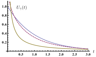
Figure 1: (Color online) The function $U_{\gamma}(t)$ for $\hat{H}=1$, and various values of $\gamma$. Dotted (blue) curve: $\gamma=0$, standard exponential function; Dashed (red) curve: $\gamma=0.1$; Solid (yellow) curve: $\gamma=0.5$.

For $\gamma=0$, the equation (10) reduces to a single (space) fractional Fokker-Planck equation

$$[\hat{p}_{4}+D_{\lambda}(\hat{\bf p}^{2})^{\lambda/2}]P({\bf x},t)=\delta^{(D)}({\bf x})\delta(t),$$ (21)

the Mittag-Leffler function reduces to $E_{1,1}(z)=\exp(z)$, and the evolution operator recovers its standard form $\hat{U}_{0}(t)=\theta(t)\exp(-t\hat{H})$. The solution, which we shall denote by $P_{X}({\bf x},t)$ for a more specific reference, is the multivariate Lévy stable distribution Nolan :

$$P_{X}({\bf x},t)=\int\frac{d^{D}p}{(2\pi)^{D}}e^{-tD_{\lambda}({\bf p}^{2})^{\lambda/2}}e^{-i{\bf p}{\bf x}}.$$ (22)

For $\lambda=2$, it reduces to the standard quantum mechanical Gaussian expression (5). For $\lambda=1$, the result is

$$\!\!\!\!P_{X}({\bf x},t)=\frac{[\Gamma(D/2+1/2)/\pi^{(D+1)/2}]D_{\lambda}t}{[(D_{\lambda}t)^{2}+|{\bf x}|^{2}]^{D/2+1/2}},$$ (23)

which is the Cauchy-Lorentz distribution function. In Fig. 2, we plot $P_{X}$ in $D=1$ dimension for $\lambda=1,1.5,2$.

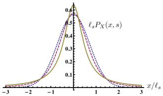
Figure 2: (Color online) Dotted (blue) curve: $\lambda=2$, standard Gaussian distribution; Dashed (red) curve: $\lambda=1.5$; Solid (yellow) curve: $\lambda=1$, Cauchy-Lorenz distribution. The length scale is $\ell_{s}=2(D_{\lambda}s)^{1/\lambda}$.

In the Appendix we provide various useful representations of $P_{X}({\bf x},t)$. At this place it is worth mentioning that this probability can be written as a superposition of Gaussian distributions $P_{\rm G}(\sigma,{\bf x})={(4\pi\sigma)^{-D/2}}e^{-{\bf x}^{2}/4\sigma}$ to be specified in Eq. (57).

II.1 Smeared-time representation, and relation between physical time $t$ and pseudotime $s$

If we use in (16) the Schwinger’s formula $1/A=\int_{0}^{\infty}\!\!ds\leavevmode\nobreak\ e^{-sA}$, we can express $P({\bf x},t)$ as an integral

$$P({\bf x},t)=\int_{0}^{\infty}\!\!\!dsP_{X}({\bf x},s)P_{T}(t,s),$$ (24)

where $P_{X}$ solves the space-fractional diffusion equation (21), with $t\equiv s$, and $P_{T}$ solves the time-fractional equation

$$[\partial_{s}+\hat{p}_{4}^{1-\gamma}]P_{T}(t,s)=\delta(t)\delta(s),$$ (25)

which encodes the relation between the pseudotime $s$ and the physical time $t$. The factorized ansatz (24) has been used previously in BarSil to solve the time-fractional Fokker-Planck equation.

For $\gamma=0$, $P_{T}(t,s)=\delta(t-s)$, and (24) reduces to $P({\bf x},t)=P_{X}({\bf x},t)$.

For $\gamma>0$, we obtain an asymmetric Lévy stable distribution REMstable

$$P_{T}(t,s)=\int_{-\infty}^{\infty}\frac{dE}{2\pi}e^{-s(-iE)^{1-\gamma}}e^{-iEt}.$$ (26)

An important feature is that $P_{T}(t,s)$ vanishes for $t<0$. This can be seen by placing the branch cut of a multivalued function $z^{1-\gamma}$ along the negative real axis, and calculating (26) as a complex integral with contour that follows the real axis, and closes in the upper half-plane. See Fig. 3 (a) where $P_{T}$ is plotted as a function of $t$ for the case $\gamma=0.03$, and various values of $s$.

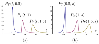
Figure 3: (Color online) (a) $P_{T}(t,s)$ as a distribution of $t$ with increasing values of the pseudotime $s=0.5,1,1.5$. (b) $P_{T}(t,s)$ as a distribution of $s$ with increasing values of the real time $t=0.5,1,1.5$. In both cases $\gamma=0.03$.

It is illustrative to view formula (24) as a smearing of the distribution $P_{X}({\bf x},s)$ around the time position $t$, defined by the probability density function $P_{T}(t,s)$. For this purpose we plot in Fig. 3 (b) $P_{T}(t,s)$ as a function of $s$, with parameter $t$ describing the position of the peak in the probability distribution.

The two plots in Fig. (3) are related through the formula

$$P_{T}(t,s)=(C/t)P_{T}(C,C^{1-\gamma}t^{\gamma-1}s),$$ (27)

which can be deduced from (26) by a simple change of the integration variable $E\rightarrow(C/t)E$. Here $C$ is an arbitrary constant. The function $P_{T}(t,s)$ as a function of two variables is shown in Figure (4).

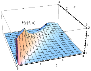
Figure 4: (Color online) $P_{T}(t,s)$ as a function of both $t$ and $s$. Here $\gamma=0.1$.

When $\gamma=0$, $P_{T}(t,s)=\delta(t-s)$ is concentrated at the point $t$, i.e., there is no smearing. For increasing $\gamma$ the peak around $t$ broadens, which can be accounted for by derivatives of the $\delta$-function. The action of $P_{T}$ on a test function $f(s)$ is

$$\int_{0}^{\infty}\!\!\!ds\leavevmode\nobreak\ P_{T}(t,s)f(s)=\sum_{n=0}^{\infty}\frac{f^{(n)}(t)}{n!}\int_{0}^{\infty}\!\!\!ds\leavevmode\nobreak\ P_{T}(t,s)(s-t)^{n}.$$ (28)

We represent $f^{(n)}(t)=(-1)^{n}\int d\tau\delta^{(n)}(\tau-t)f(\tau)$, and calculate

$$\int_{0}^{\infty}\!\!\!\!\!dsP_{T}(t,s)s^{k}\!=\!\!\int\!\frac{dE}{2\pi}\frac{e^{-iEt}k!}{(-iE)^{(1-\gamma)(k+1)}}\!=\!\frac{k!\theta(t)t^{(1-\gamma)k-\gamma}}{\Gamma[(1\!-\!\gamma)(k\!+\!1)]}$$ (29)

to find that

$$P_{T}(t,s)=\sum_{n=0}^{\infty}\frac{t^{n}}{n!}c_{n}(t)\delta^{(n)}(s-t),$$ (30)

where

$$c_{n}(t)=\sum_{k=0}^{n}{n\choose k}(-1)^{k}\frac{k!\theta(t)t^{-\gamma(k+1)}}{\Gamma[(1-\gamma)(k+1)]}.$$ (31)

In view of these relations, the equation (24) translates into

$$P({\bf x},t)=\sum_{n=0}^{\infty}\frac{(-t)^{n}}{n!}c_{n}(t)\partial_{t}^{n}P_{X}({\bf x},t).$$ (32)

One can easily verify that for $\gamma=0$, $c_{n}=\delta_{n0}$, and $P({\bf x},t)=P_{X}({\bf x},t)$.

II.2 Fox $H$-function representation of the Green function

Solution of the double fractional equation (10) has been obtained previously in terms of the Fox H-function DUAN . We derive the same result starting from formula (24), where we consider the representation (60) of $P_{X}({\bf x},s)$. Integration over the pseudotime $s$ can be performed, followed by the $E$ integration, that yields

$$P({\bf x},t)=\!\!\frac{t^{-\gamma}}{\pi^{D/2}|{\bf x}|^{D}}H^{2,1}_{2,3}\left(\!\left[\frac{|{\bf x}|}{\ell_{t}}\right]^{\lambda}\bigg{|}^{(1,1);(1-\gamma,1-\gamma)}_{(1,1),(D/2,\lambda/2);(1,\lambda/2)}\!\right)\!.$$ (33)

Here $\ell_{t}\equiv 2(D_{\lambda}t^{1-\gamma})^{1/\lambda}$ is a $t$-dependent length scale, and $H^{2,1}_{2,3}$ is the Fox $H$-function FH ; Mathai , defined by the contour integral

$$\frac{P({\bf x},t)|{\bf x}|^{D}}{t^{-\gamma}\pi^{-D/2}}\!=\!\!\!\int_{\cal C}\frac{dz}{2\pi i}\frac{\Gamma(1+z)\Gamma(\frac{D}{2}+\frac{\lambda}{2}z)\Gamma(-z)}{\Gamma(-\frac{\lambda}{2}z)\Gamma(1\!-\!\gamma+(1\!-\!\gamma)z)}\!\!\left[\frac{|{\bf x}|^{\lambda}}{\ell_{t}^{\lambda}}\right]^{-z}\!\!\!\!,$$ (34)

where the contour ${\cal C}$ runs from $-i\infty$ to $+i\infty$. In Fig. 5 we show how values of $\gamma>0$ modify the Gaussian distribution (for which $\lambda=2$, $\gamma=0$).

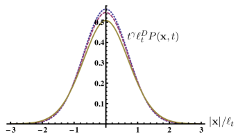
Figure 5: (Color online) In all cases $\lambda=2$. Dotted (blue) curve: $\gamma=0$, standard Gaussian distribution; Dashed (red) curve: $\gamma=0.03$; Solid (yellow) curve: $\gamma=0.1$.

The large-$|{\bf x}|$ asymptotics of (33) is governed by the pole of the integrand at $z=1$:

$$t^{\gamma}|{\bf x}|^{D}P({\bf x},t)\overset{|{\bf x}|\rightarrow\infty}{\approx}\frac{\ell_{t}^{\lambda}}{|{\bf x}|^{\lambda}}\frac{-\Gamma(\frac{D+\lambda}{2})}{\pi^{D/2}\Gamma(2-2\gamma)\Gamma(-\frac{\lambda}{2})}.$$ (35)

Analysis of the small-$|{\bf x}|$ behavior is more subtle due to a richer pole structure of the integrand in (34) (see Kilbas ). If we assume only simple poles, we can extract the leading behavior

$$t^{\gamma}P({\bf x},t)\overset{|{\bf x}|\rightarrow 0}{\approx}\left\{\begin{array}[]{ll}A(t)+B(t)|{\bf x}|^{2\lambda-D},&2\lambda-D<2\\ A(t)+{\cal O}[|{\bf x}|^{2}](t),&2\lambda-D>2\end{array}\right.,$$ (38)

with

$$\!\!\!\!\!\!\!\!\!A(t)\! = \!\frac{\pi^{1-D/2}\ell_{t}^{-D}2/\lambda}{\sin(\pi\frac{D}{\lambda})\Gamma(\frac{D}{2})\Gamma[\frac{(1-\gamma)(\lambda-D)}{\lambda}]},$$ (39)

$$\!\!\!\!\!\!\!\!\!B(t)\! = \!-\frac{\pi^{-D/2}\Gamma(\frac{D}{2}-\lambda)}{\Gamma(\lambda)\Gamma(\gamma-1)\ell_{t}^{2\lambda}}.$$ (40)

In particular, for $2\lambda<D$ the value of $P({\bf x},t)$ tends to either $+\infty$ or $-\infty$ as $|{\bf x}|\rightarrow 0$. See Fig. 6.

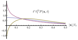
Figure 6: (Color online) Dotted (blue) curve: $\gamma=0,\lambda=1$, Cauchy-Lorentz distribution; Dashed (red) curve: $\gamma=0.1,\lambda=1$; Solid (yellow) curve: $\gamma=-0.1,\lambda=1$, assumes negative values. Here D=3.

III Path-integral formulation

We note that the probability (15) may be calculated from the doubly fractional canonical path integral over fluctuating orbits $t(s),{\bf x}(s)$ $p_{4}(s),{\bf p}(s)$ viewed as functions of some pseudotime $s$ REM1 :

$$\{{\bf x}_{b}t_{b}s_{b}|{\bf x}_{a}t_{s}s_{a}\}=\int{\cal D}{\bf x}{\cal D}t{\cal D}{\bf p}{\cal D}p_{4}e^{{\cal A}},$$ (41)

with ${\cal A}$ being the euclidean action of the paths $t(s),{\bf x}(s)$:

$${\cal A}=\int ds[i({\bf p}{\bf x}^{\prime}-ip_{4}t^{\prime})-{\cal H}({\bf p},p_{4})].$$ (42)

Here $t^{\prime}(s)\equiv dt(s)/ds$, ${\bf x}^{\prime}(s)\equiv d{\bf x}(s)/ds$, and ${\cal H}({\bf p},p_{4})=p_{4}^{1-\gamma}+D_{\lambda}(\hat{\bf p}^{2})^{\lambda/2}$. At each $s$, the integrals over the components of ${\bf p}(s)$ run from $-\infty$ to $\infty$, whereas those over $p_{4}(s)$ run from $-i\infty$ to $i\infty$. To obtain the distribution $P({\bf x},t)$, we finally form the integral

$$P({\bf x},t)=\int_{0}^{\infty}ds\{{\bf x}\,t\,s|{\bf 0}\,0\,0\}.$$ (43)

This is analogous to prescription (24) which links solutions of the space- and time-fractional diffusion equations (21) and (25).

If $\gamma=0$, the path integral over $p_{4}(s)$ yields the functional $\delta[t^{\prime}(s)-1]$, which ensures that $dt$ and $ds$ increments are equal. This brings (41) to the canonical path integral

$$({\bf x}_{b}t_{b}|{\bf x}_{a}t_{a})=\int{\cal D}{\bf x}{\cal D}{\bf p}e^{{\cal A}^{\prime}},$$ (44)

with

$${\cal A}^{\prime}=\int d\tau[i{\bf p}\dot{\bf x}-D_{\lambda}(\hat{\bf p}^{2})^{\lambda/2}].$$ (45)

Now $P({\bf x},t)=({\bf x}t|{\bf 0}\,0)$ satisfies the ordinary fractional Fokker-Planck equation

$$[\hat{p}_{4}+D_{\lambda}(\hat{\bf p}^{2})^{\lambda/2}]P({\bf x},t)=\delta(t)\delta^{(D)}({\bf x}),$$ (46)

which has been discussed at length in recent literature LASKIN .

IV Langevin equations and computer simulations

In the past, many nontrivial Schrödinger equations (for instance that of the $1/r$-potential) have been solved with path integral methods by re-formulating them on the pseudotime axis $s$, that is related to the time $t$ via a space-dependent differential equation $t^{\prime}(s)=f(x(t))$. This method was invented by Duru and Kleinert DK to solve the path integral of the hydrogen atom, and has recently been applied successfully to various Fokker-Planck equations DW ; TEMP . The stochastic differential equation (49), that connects pseudotime $s$ and the physical time $t$, may be seen as a stochastic version of the Duru-Kleinert transformation that promises to be a useful tool to study non-Markovian systems.

Certainly, the solutions of Eq. (46) can also be obtained from a stochastic differential equation

$$\dot{\bf x}=\mbox{\boldmath$\eta$},$$ (47)

whose noise is distributed with a fractional probability

$$P[\mbox{\boldmath$\eta$}]=\int\!{\cal D}^{D}\!pe^{\int\!dt(i{\bf p}\cdot\mbox{\scriptsize\boldmath$\eta$}-D_{\lambda}({\bf p}^{2})^{\lambda/2})}.$$ (48)

Simulating this stochastic differential equation on a computer, we confirm the analytic form (22) of $P_{X}({\bf x},s)=P({\bf x},t)$ for $\gamma=0$. See Fig. 7 (a).

Analogously, the solution of Eq. (25) can also be obtained from a SDE

$$t^{\prime}(s)=\eta_{T}(s),$$ (49)

with noise distribution

$$P[\eta_{T}]=\int\!{\cal D}\!p_{4}e^{\int\!ds(p_{4}\eta_{T}-(p_{4})^{1-\gamma})},$$ (50)

and compared with the result (26) for $P_{T}(t,s)$. See Fig. 7 (b).

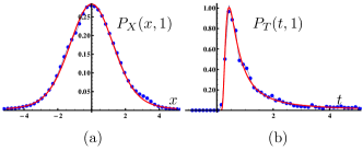
Figure 7: (Color online) Comparison of analytic (solid red curve) and numerical (blue circles) results for the distribution function $P_{X}(x,s\!\!=\!\!1)$ in $D=1$ dimension (a), and $P_{T}(t,s\!\!=\!\!1)$ for $\gamma=0.3$ (b). In each case an average has been taken over $5000$ representative trajectories of stochastic differential equations (47) and (49), with $10$ time steps $\Delta s=0.1$.

Solution of the double fractional Fokker-Planck equation (10) can be obtained, in view of the relation (43) (or (24)), by simulating (47) for $t\equiv s$ and (49), and letting the final value of the pseudotime $s$ be random. This yields a probability distribution $P({\bf x},t)$. In Fig. 8 we compare the results of a computer simulation with the analytic form (34) by plotting $P({\bf x},t)$ as a function of ${\bf x}$ for various values of time $t$. Since the distribution $P({\bf x},t)$ itself is not normalized, but rather

$$\int d^{D}xP({\bf x},t)=\int_{0}^{\infty}\!\!\!dsP_{T}(t,s)=\frac{\theta(t)t^{-\gamma}}{\Gamma(1-\gamma)},$$ (51)

we define a renormalized version $\overline{P}({\bf x},t)=P({\bf x},t)/\int d^{D}xP({\bf x},t)$.

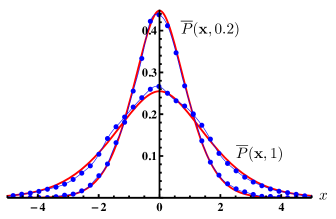
Figure 8: (Color online) Comparison of computer simulation and the renormalized exact solution $\overline{P}({\bf x},t)$ for t=0.2,1.

V Summary

Summarizing, we have seen that a many-body system with strong couplings between the constituents satisfies a more general form of the Schrödinger equation, in which the momentum and the energy appear with a power different from $\lambda=2$ and $\gamma=0$, respectively. We have calculated the associated Green functions and discussed their properties and their representations. We pointed out that these Green functions can be written as path integrals over fluctuating time and space orbits that are functions of some pseudotime $s$. This is a Markovian object, but non-Markovian in the physical time $t$. The non-Markovian character is caused by the fact that function $t(s)$ follows a stochastic differential equation of the Langevin type.

The particle distributions can also be obtained by solving a Langevin type of equation in which the noise has correlation functions whose probability distribution is specified by an equation like (48).

The Green functions whose theory was presented here will play an important role in the development of an interacting theory of fields whose worldlines contain non-Gaussian random walks displaying extremely large deviations from their avarages.

Acknowledgment: We are grateful to P. Jizba, and A. Pelster for useful comments. V.Z. received support from GAČR Grant No. P402/12/J077.

Appendix 1: Fractional differential operators that enter the general fractional Fokker-Planck equation (7) are defined through formula (14). Using $e^{-\sigma\hat{\bf p}^{2}}\delta({\bf x})=(4\pi\sigma)^{-D/2}e^{-{\bf x}^{2}/(4\sigma)}$, and $e^{-\sigma\hat{p}_{4}}\delta(t)=\delta(t-\sigma)$, we derive the following relations,

$$|{\bf x}|^{\lambda} = \frac{\pi^{D/2}\Gamma(\frac{\lambda+D}{2})}{2^{-\lambda-D}\Gamma(-\frac{\lambda}{2})}(\hat{\bf p}^{2})^{-(\lambda+D)/2}\delta^{(D)}({\bf x}),$$ (52)

$$\theta(t)t^{\alpha} = \Gamma(\alpha+1)(\hat{p}_{4})^{-\alpha-1}\delta(t),$$ (53)

which we can substitute into (33), (34) in order to verify that these satisfy the equation (10). We first obtain

$$P({\bf x},t)=\int_{\cal C}\frac{dz}{2\pi i}\Gamma(1+z)\Gamma(-z)D_{\lambda}^{z}(\hat{\bf p}^{2})^{\lambda z/2}$$

$$\times(\hat{p}_{4})^{(\gamma-1)(z+1)}\delta^{(D)}({\bf x})\delta(t),$$ (54)

which can be pole-expanded to yield

$$\sum_{n=0}^{\infty}(-D_{\lambda})^{n}(\hat{\bf p}^{2})^{\lambda n/2}(\hat{p}_{4})^{(\gamma-1)(n+1)}\delta^{(D)}({\bf x})\delta(t).$$ (55)

Summing up this geometric series, we arrive at

$$P({\bf x},t)=[\hat{p}_{4}^{1-\gamma}+D_{\lambda}(\hat{\bf p}^{2})^{\lambda/2}]^{-1}\delta^{(D)}({\bf x})\delta(t).$$ (56)

Appendix 2: We derive several expressions for the solution $P_{X}({\bf x},s)$ of (21), starting from the representation (22).

On expanding the exponential, and representing the powers as $({\bf p}^{2})^{\lambda n/2}=\Gamma[-\lambda n/2]^{-1}\int_{0}^{\infty}\frac{d\sigma}{\sigma}\sigma^{-\lambda n/2}e^{-\sigma{\bf p}^{2}}$, the momentum integration yields the superposition of Gaussian expression

$$P_{X}({\bf x},s)=\int_{0}^{\infty}\frac{d\sigma}{\sigma}f_{\lambda}(\sigma)P_{G}({\bf x},D_{\lambda}^{2/\lambda}s^{2/\lambda}\sigma),$$ (57)

with weight

$$f_{\lambda}(\sigma)=\sum_{n=0}^{\infty}\frac{(-1)^{n}\sigma^{-\lambda n/2}}{n!\Gamma(-\lambda n/2)}.$$ (58)

To prove this, we perform the $\sigma$-integration term by term, using the formula $\int_{0}^{\infty}\frac{d\sigma}{\sigma}\sigma^{-\nu}e^{-a/\sigma}=\Gamma(\nu)/a^{\nu}$, and obtain the large-$|{\bf x}|$ expansion

$$P_{X}({\bf x},s)=\frac{1}{\pi^{D/2}|{\bf x}|^{D}}\sum_{n=0}^{\infty}\frac{(-1)^{n}\Gamma(\frac{\lambda n+D}{2})}{n!\Gamma(-\lambda n/2)}\left[\frac{\ell_{s}^{\lambda}}{|{\bf x}|^{\lambda}}\right]^{n}\!\!\!,$$ (59)

where $\ell_{s}=2(D_{\lambda}s)^{1/\lambda}$. The series can also be viewed as a pole expansion of the contour integral, and hence

$$P_{X}({\bf x},s)=\frac{1}{\pi^{D/2}|{\bf x}|^{D}}\int_{\cal C}\frac{dz}{2\pi i}\frac{\Gamma(\frac{\lambda z+D}{2})\Gamma(-z)}{\Gamma(-\lambda z/2)}\left[\frac{|{\bf x}|^{\lambda}}{\ell_{s}^{\lambda}}\right]^{-z}\!\!\!,$$ (60)

with the contour ${\cal C}$ running from $-i\infty$ to $+i\infty$. From this, the expansion (59) arises by enclosing the right complex half-plane and calculating the residua of the integrand, using ${\rm Res}(\Gamma(az+b),-(n+b)/a)=(-1)^{n}/(n!a)$. A small-$|{\bf x}|$ expansion of (60) is obtained by closing the integration contour in the left half-plane, leading to

$$P_{X}({\bf x},s)=\sum_{n=0}^{\infty}\frac{(-1)^{n}2/\lambda}{\pi^{D/2}\ell_{s}^{D}}\frac{\Gamma(\frac{2n+D}{\lambda})}{n!\Gamma(\frac{D}{2}+n)}\!\left[\frac{|{\bf x}|^{2}}{\ell_{s}^{2}}\right]^{n}.$$ (61)

The series (59) and (61) are convergent, or asymptotic, or even trivially zero, depending on the parameter $\lambda$.

References

- (1) W. Feller An Introduction to Probability Theory and Its Applications vol. 2, Wiley, New York, 1991; J.-P. Bouchaud and M. Potters, Theory of Financial Risks, From Statistical Physics to Risk Management, Cambridge U. Press, 2000. See also Ch. 20 in PI .
- (2) F. Black and M. Scholes, J. Pol. Economy 81, 637 (1973).
- (3) The theory has been reviewed in many detailed publications, our notation follows the textbook PI .
- (4) H. Kleinert, Path Integrals in Quantum Mechanics, Statistics, Polymer Physics, and Financial Markets, World Scientific, Singapore, 2006.
- (5) T. Preis, Econophysics in a Nutshell, Science & Culture 76, 333-337 (2010)
- (6) R. N. Mantegna, H. E. Stanley, Introduction to Econophysics: Correlations and Complexity in Finance, Cambridge University Press (2000)
- (7) B. Podobnik, P. Ch. Ivanov, Y. Lee, A. Chessa and H. E. Stanley, Europhys. Lett. 50 711 (2000) (arXiv:cond-mat/9910433)
- (8) A travelling pedestrian salesman is a Gaussian random walker, as a jetsetter he becomes a Lévy random walker.
- (9) See http://en.wikipedia.org/wiki/Black_swan_theory
- (10) The concept of a Hamiltonian in the theory of statistical distributions was introduced in the textbook PI . It has its root in the path integral formulation of quantum mechanics and emphasizes the fact that in this formulation particles run along fluctuating world lines in spacetime, where they perform random walks with distributions that may be Gaussian or nongaussian depending on the form of the Hamiltonian as functions of the momentum . The distributions solve a Fokker-Planck equation of the type (7), driven by differential operator that is obtained by replacing the momentum in the Hamiltonian by the differential operator .
- (11) C. Nardini, S. Gupta, S. Ruffo, T. Dauxois, and F. Bouchet, J. Stat. Mech. (2012) L01002 (http://arxiv.org/pdf/1111.6833.pdf)
- (12) R. E. Angulo, V. Springel, S. D. M. White, A. Jenkins, C. M. Baugh, C. S. Frenk, Monthly Notices of the Royal Astronomical Society 426: 2046–2062 (2012) (arXiv:1203.3216).
- (13) Du Jiulin, 2004 Europhys. Lett. 67, 893 (2004), Phys. Lett. A 329, 262(2004).
- (14) J. Einasto, (arXiv:1109.5580).
- (15) F. Boettcher, C. Renner, H.P. Waldl, J. Peinke, Boundary-Layer Meteorology (2003) Volume 108, Issue 1, pp 163-173 (arXiv:physics/0112063).
- (16) P. Bhattacharyya, A. Chatterjee, B.K. Chakrabarti, Physica A 381, 377 (2007) (arXiv:physics/0510038) .
- (17) S. Umarov, C. Tsallis, M. Gell-Mann, and S. Steinberg, J. Math. Phys. 51, 033502 (2010) (http://arxiv.org/abs/cond-mat/0606040).
- (18) Note that the function is the functional Fourier transform of the Hamiltonian (1) that drives the Fokker-Planck equation (7). See Eq. (20.153) in Ref. PI .
- (19) M.F. Shlesinger, G.M. Zaslavsky, U. Frish (Eds.), Lévy Flights and Related Topics in Physics, LNP 450 (1995).
- (20) R. Kutner, A. Pekalski, K. Sznajd-Weron (Eds.), Anomalous Diffusion From Basics to Applications, LNP 519 (1999).
- (21) T. Srokowski, Phys. Rev. E 79, 040104(R) (2009).
- (22) Fokker-Planck equations in which only the time derivative has a fractional power have been studied in R. Metzler and J. Klafter, Physics Reports 339 1-77 (2000).
- (23) H. Kleinert and V. Schulte-FrohlindeV. Schulte-Frohlinde, Critical Phenomena in -Theory, World Scientific, Singapore, 2001 (http://klnrt.de/b8).
- (24) H. Kleinert, EPL 100, 10001 (2012) (http://klnrt.de/399/399-TAIPEH.pdf). H. Kleinert, (http://klnrt.de/403).
- (25) M. M. Meerschaert, A. Sikorskii, Stochastic Models for Fractional Calculus, Walter de Gruyter (2011).
- (26) G. M. Zaslavsky, Hamiltonian Chaos and Fractional Dynamics, OUP Oxford (2005).
- (27) R. Hilfer (Ed.), Applications of Fractional Calculus in Physics, World Scientific (2000).
- (28) E. Barkai, R. Metzler, and J. Klafter, Phys. Rev. E 61, 132–138 (2000).
- (29) R.P. Feynman, Phys. Rev. 80, 440 (1950); R. P. Feynman and A.R. Hibbs, Quantum Mechanics and Path Integrals (McGraw-Hill, New York, 1965).
- (30) For the so-called Riesz fractional derivative see R. Metzler, E. Barkai, J. Klafter, Phys. Rev. Lett. 82, 3564 (1999); B.J. West, P. Grigolini, R. Metzler, and T.F. Nonnenmacher, Phys.Rev. E 55, 99 (1997). For the so-called Weyl derivative. See R.K. Raina and C.L. Koul, Proc. Am. Math. Soc. 73, 188 (1979).
- (31) The relevant functional matrix is = , where and . If is close to an even integer, it needs a small positive shift and we can replace by , where . For we have with , so that we find .
- (32) I. S. Gradshteyn and I. M. Ryzhik, Table of Integrals, Series, and Products, Seventh Edition, Elsevier (2007), Formula
- (33) A. Erdélyi, W. Magnus, F. Oberhettinger, and F. Tricomi, Higher Transcendental Functions, Vol. 3, New York (1981), pp. 206-212.
- (34) H. J. Haubold, A. M. Mathai, and R. K. Saxena, J. Appl. Math. 298628 (2011).
- (35) More generally, can be a generic time-independent Hamiltonian. In particular, it may contain an additional potential term.
- (36) Nolan, J. P., Multivariate stable distributions: approximation, estimation, simulation and identification. In R. J. Adler, R. E. Feldman, and M. S. Taqqu (Eds.), A Practical Guide to Heavy Tails, pp. 509-526, Birkhauser, Boston (1998).
- (37) E. Barkai and R. J. Silbey, J. Phys. Chem. B, 104 (16), pp 3866–3874 (2000).
- (38) Lévy distributions are implemented in Wolfram Mathematica 8 under the command StableDistribution.
- (39) Jun-Sheng Duan, J. Math. Phys. 46, 013504 (2005).
- (40) C. Fox, Trans. Amer. Math. Soc. 98, 395 (1961).
- (41) A. M. Mathai, R. K. Saxena, H. J. Haubold, The H function: Theory and Applications, Springer, 2010.
- (42) A. A. Kilbas and M. Saigo, Journal of Applied Math. and Stoch. Anal., 12 2 191-204 (1999).
- (43) This technique is explained in Chapters 12 and 19 of Ref. PI . The pseudotime resembles the so-called Schwinger proper time used in relativistic physics.
- (44) N. Laskin, (arXiv/1009.5533); Phys.Lett. A 268, 298 (2000); Phys. Rev. E 62, 3135 (2000); (ibid.) E 66, 056108 (2002); Chaos 10, 780 (2000); Communications in Nonlinear Science and Numerical Simulation 12, 2 (2007).
- (45) I.H. Duru and H. Kleinert, Phys. Lett. B 84, 30 (1979) (klnrt.de/65/65.pdf); Fortschr. Phys. 30, 401 (1982) (klnrt.de/83/83.pdf). See also Chaps. 13 and 14 in PI .
- (46) A. Young and C. DeWitt-Morette, Ann. Phys. (N.Y.) 169, 140 (1984); H. Kleinert and A. Pelster, Phs. Rev. Lett. 78, 565 (1997).
- (47) L.Z.J. Liang, D. Lemmens, and J. Tempere, Phys. Rev. E 83, 056112 (2011) (arxiv:1101.3713).