New bounds on the Lebesgue constants of Leja sequences on the unit disc and on $\Re$-Leja sequences.

Abstract

In the papers [6, 7] we have established linear and quadratic bounds, in $k$, on the growth of the Lebesgue constants associated with the $k$-sections of Leja sequences on the unit disc ${\cal U}$ and $\Re$-Leja sequences obtained from the latter by projection into $[-1,1]$. In this paper, we improve these bounds and derive sub-linear and sub-quadratic bounds. The main novelty is the introduction of a “quadratic” Lebesgue function for Leja sequences on ${\cal U}$ which exploits perfectly the binary structure of such sequences and can be sharply bounded. This yields new bounds on the Lebesgue constants of such sequences, that are almost of order $\sqrt{k}$ when $k$ has a sparse binary expansion. It also yields an improvement on the Lebesgue constants associated with $\Re$-Leja sequences.

1 Introduction

The growth of the Lebesgue constant of Leja sequences on the unit disc and $\Re$-Leja sequences was first studied in [3, 4]. The main motivation was the study of the stability of Lagrange interpolation in multi-dimension based on intertwining of block unisolvent arrays. Such sequences, more particularly $\Re$-Leja sequences, were also considered in many other works in the framework of structured hierarchical interpolation in high dimension. Although not always referred to as such, they are typically considered in the framework of sparse grids for interpolation and quadrature [10, 11]. Indeed, the sections of length $2^{n}+1$ of $\Re$-Leja sequences coincide with the Clenshaw-Curtis abscissas $\cos(2^{-n}j\pi),j=0,\dots,2^{n}$ which are de facto used, thanks to the logarithmic growth of their Lebesgue constant.

Motivated by the development of cheap and stable non-intrusive methods for the treatment of parametric PDEs in high dimension, we have also used these sequences in [9, 5] with a highly sparse hierarchical polynomial interpolation procedure. The multi-variate interpolation process is based on the Smolyak formula and the sampling set is progressively enriched in a structured infinite grid $\otimes_{j=0}^{d}Z$ together with the polynomial space by only one element at a time. The Lebesgue constant that quantifies the stability of the interpolation process depends naturally on the sequence $Z$. We have shown in [7] that it has quadratic and cubic bounds in the number of points of interpolation when $Z$ is a Leja sequence on ${\cal U}$ or an $\Re$-Leja sequence, thanks to the linear and quadratic bounds on the growth of the Lebesugue constant of such sequences, also established in [6, 7]. We refer to the introduction and section $2$ in [7] for a concise description on the construction of the interpolation process and the study of its stability.

The present paper is also concerned with the growth of the Lebesgue constant of Leja and $\Re$-Leja sequences. We improve the linear and quadratic bounds obtained in [7]. In particular, we show that for $\Re$-Leja sequnences, the bound is logarithmic for many values of $k$ which may be useful for proposing cheap and stable interpolation scheme in the framework of sparse grids [11].

1.1 One dimensional hierarchical interpolation

Let $X$ be a compact domain in $\mathbb{C}$ or $\mathbb{R}$, typically the complex unit disc ${\cal U}:=\{|z|\leq 1\}$ or the unit interval $[-1,1]$, and $Z=(z_{j})_{j\geq 0}$ a sequence of mutually distinct points in $X$. We denote by $I_{Z_{k}}$ the univariate interpolation operator onto the polynomials space ${\mathbb{P}}_{k-1}$ associated with the section of length $k$, $Z_{k}:=(z_{0},\cdots,z_{k-1})$. The interpolation operator is given by Lagrange interpolation formula: for $f\in{\cal C}(X)$ and $z\in X$

$$I_{Z_{k}}f(z)=\sum_{j=0}^{k-1}f(z_{j})l_{j,k}(z),\quad\quad l_{j,k}(z):=\prod_{i=0\atop i\neq j}^{k-1}\frac{z-z_{j}}{z_{i}-z_{j}},\;\;j=0,\dots,k-1.$$ (1.1)

Since the sections $Z_{k}$ are nested, it is convenient to give the operator $I_{Z_{k}}$ using Newton interpolation formula which amounts essentially writing: $\Delta_{0}f:=I_{Z_{1}}f\equiv f(z_{0})$ and

$$I_{Z_{k+1}}=I_{Z_{k}}+\Delta_{k}=\sum_{l=0}^{k}\Delta_{l},\quad\mbox{where}\quad\Delta_{l}(Z):=I_{Z_{l+1}}-I_{Z_{l}},\;\;l\geq 1,$$ (1.2)

and computing the operators $\Delta_{l}$ using divided differences, see [12, Chapter 2] or equivalently the following formula which are differently normalized, see [7, 9],

$$\Delta_{l}f=\Bigl{(}f(z_{l})-I_{Z_{l}}f(z_{l})\Bigr{)}\prod_{j=0}^{l-1}\frac{(z-z_{j})}{(z_{l}-z_{j})},\quad l\geq 1,$$ (1.3)

The stability of the operator $I_{Z_{k}}$ depends on the positions of the elements of $Z_{k}$ on $X$, in particular through the Lebesgue constant associated with $Z_{k}$, defined by

$$\mathbb{L}_{Z_{k}}:=\max_{f\in C(X)-\{0\}}\frac{\|I_{Z_{k}}f\|_{L^{\infty}(X)}}{\|f\|_{L^{\infty}(X)}}=\max_{z\in X}\lambda_{Z_{k}}(z),$$ (1.4)

where $\lambda_{Z_{k}}$ is the so-called Lebesgue function associated with $Z_{k}$ defined by

$$\lambda_{Z_{k}}(z):=\sum_{i=0}^{k-1}|l_{i,k}(z)|,\quad\quad z\in X.$$ (1.5)

We also introduce the notation

$$\mathbb{D}_{k}(Z):=\max_{f\in C(X)-\{0\}}\frac{\|\Delta_{k}f\|_{L^{\infty}(X)}}{\|f\|_{L^{\infty}(X)}}.$$ (1.6)

In the case of the unit disk or the unit interval, it is known that $\mathbb{L}_{k}$ the Lebesgue constant associated with any set of $k$ mutually distinct points can not grow slower than $\frac{2\log(k)}{\pi}$ and it is well known that such growth is fulfilled by the set of $k$-roots of unity in the case $X={\cal U}$ and the Tchybeshev or Gauss-Lobatto abscissas in the case $X=[-1,1]$, see e.g. [2]. However such sets of points are not the sections of a fixed sequence $Z$.

In [3, 4], the authors considered for $Z$ Leja sequences on ${\cal U}$ initiated at the boundary $\partial{\cal U}$ and $\Re$-Leja sequences obtained by projection onto $[1,1]$ of the latter when initiated at $1$. They showed that the growth of $\mathbb{L}_{Z_{k}}$ is controlled by ${\cal O}(k\log(k))$ and ${\cal O}(k^{3}\log(k))$ respectively. In our previous works [6, 7], we have improved these bounds to $2k$ and $8\sqrt{2}k^{2}$ respectively. We have also established in [7] the bound ${\mathbb{D}}_{k}\leq(1+k)^{2}$ for the difference operator, which could not be obtained directly from ${\mathbb{D}}_{k}\leq\mathbb{L}_{Z_{k+1}}+\mathbb{L}_{Z_{k}}$ and which is essential to prove that the multivariate interpolation operator using $\Re$-Leja sequences has a cubic Lebesgue constant, see [7, formula 25].

1.2 Contributions of the paper

In this paper, we improve the bounds of the previous paper [3, 4, 6, 7]. Our techniques of proof share several points with those developed in [6, 7], yet they are shorter and relies notably on the binary pattern of Leja sequences on the unit disk. The novelty in the present paper is the introduction of the “quadractic” Lebesgue constant

$$\lambda_{Z_{k},2}(z):=\Bigl{(}\sum_{i=0}^{k-1}|l_{i,k}(z)|^{2}\Bigr{)}^{\frac{1}{2}},\quad z\in X,$$ (1.7)

where $l_{i,k}$ are the Lagrange polynomials as defined in (1.5). We study this function and its maximum

$$\mathbb{L}_{Z_{k},2}:=\max_{z\in X}\lambda_{Z_{k},2}(z).$$ (1.8)

We establish in §2 in the case where $Z$ is any Leja sequence on ${\cal U}$ initiated on the boundary $\partial{\cal U}$ the “sharp” inequality

$$\lambda_{Z_{k}}(z_{k})\leq\mathbb{L}_{Z_{k},2}\leq 3\lambda_{Z_{k}}(z_{k}),\quad{and}\quad\lambda_{Z_{k}}(z_{k}):=\sqrt{2^{\sigma_{1}(k)}-1},$$ (1.9)

where $\sigma_{1}(k)$ denote the number of ones in the binary expansion of $k$. Cauchy-schwatrz inequality applied to the Lebesgue function $\lambda_{Z_{k}}$ defined in (1.5) yields $\lambda_{Z_{k}}\leq\sqrt{k}~{}\lambda_{Z_{k},2}$. This shows that we also establish

$$\mathbb{L}_{Z_{k}}\leq 3\sqrt{k}~{}\sqrt{2^{\sigma_{1}(k)}-1},$$ (1.10)

for Leja sequences on ${\cal U}$, which improves considerably the linear bound $2k$ established in [6] when the binary expansion of $k$ is very sparse. For example, for $k=2^{n}+3$ with $n$ large, we get $\mathbb{L}_{Z_{k}}\leq 3\sqrt{7k}<<k$. Using the bound (1.9), we establish in §3 a new bound on the growth of Lebesgue constants of $\Re$-Leja sequences that implies

$$\mathbb{L}_{k}\leq 6\sqrt{5}~{}k~{}2^{\sigma_{1}(l)},\quad\mbox{where}\quad l=k-(2^{n}+1),$$ (1.11)

where $n$ is the integer such that $2^{n}+1\leq k<2^{n+1}+1$. Again, we remark that the previous bound improves the bound $8\sqrt{2}k^{2}$ established in [7] when $l$ is small compared to $2^{n}$ or very sparse in the sense of binary expansion. We actually prove a bound that is logarithmic for many values of $k$ other than the values $2^{n}+1$, see Theorem 3.2.

Finally, we provide in §4 new bounds on the growth of $\mathbb{D}_{k}$ the norm of the difference operators. We provide the bounds

$$\mathbb{D}_{k}\leq 1+\sqrt{k(2^{\sigma_{1}(k)}-1)},\quad\quad\mathbb{D}_{k}\leq 2^{\sigma_{1}(k)}2^{n},\quad k\geq 1.$$ (1.12)

in the case of Leja sequences on ${\cal U}$ and the case of $\Re$-Leja sequences respectively where for the latter $n$ is defined as above.

1.3 Notation

In the remainder of the paper, we work with the following notation. For an infinite sequence $Z:=(z_{j})_{j\geq 0}$ on $X$, we introduce the section $Z_{l,m}:=(z_{l},\cdots,z_{m-1})$ for any $l\leq m-1$. Given two finite sequences $A=(a_{0},\dots,a_{k-1})$ and $B=(b_{0},\dots,b_{l-1})$, we denote by $A\wedge B$ the concatenation of $A$ and $B$, i.e. $A\wedge B=(a_{0},\dots,a_{k-1},b_{0},\dots,b_{l-1})$. For any finite set $S=(s_{0},\cdots,s_{k-1})$ of complex numbers and $\rho\in\mathbb{C}$, we introduce the notation

$$\rho S:=(\rho s_{0},\cdots,\rho s_{k-1}),\quad\Re(S):=(\Re(s_{0}),\cdots,\Re(s_{k-1})),\quad\overline{S}:=(\overline{s_{0}},\cdots,\overline{s_{k-1}}).$$ (1.13)

Throughout this paper, to any finite set $S$ of numbers, we associate the polynomial

$$w_{S}(z):=\prod_{s\in S}(z-s),\quad\mbox{with the convention}\quad w_{\emptyset}(z):=1$$ (1.14)

Any integer $k\geq 1$ can be uniquely expanded according to

$$k=\sum_{j=0}^{n}a_{j}2^{j},\quad a_{j}\in\{0,1\}$$ (1.15)

We denote by $\sigma_{1}(k)$, $\sigma_{0}(k)$ the number of ones and zeros in the binary expansion of $k$ and by $p(k)$ the largest integer $p$ such that $2^{p}$ divide $k$. For $k=2^{n},\dots,2^{n+1}-1$ with binary expansion as above, one has

$$\sigma_{1}(k)=\sum_{j=0}^{n}a_{j}\quad\mbox{and}\quad\sigma_{0}(k)=\sum_{j=0}^{n}(1-a_{j})=n+1-\sigma_{1}(k).$$ (1.16)

We should finally note that, unless stated otherwise, we only work with complex numbers $z$ belonging to the unit circle $\partial{\cal U}$. This is because in the complex setting we investigate supremums of sub-harmonic functions, $\lambda_{Z_{k}}$ and $\lambda_{Z_{k},2}$, which is always attained on the boundary.

2 Leja sequences on the unit disk

Leja sequences $E=(e_{j})_{j\geq 0}$ on $\cal U$ considered in [3, 4, 6, 7] have all their initial value $e_{0}\in\partial\cal U$ the unit circle. They are defined inductively by picking $e_{0}\in\partial{\cal U}$ arbitrary and defining $e_{k}$ for $k\geq 1$ by

$$e_{k}={\rm argmax}_{z\in\cal U}|z-e_{k-1}|\dots|z-e_{0}|.$$ (2.1)

The maximum principle implies that $e_{j}\in\partial\cal U$ for any $j\geq 1$. Also, the previous ${\rm argmax}$ problem might admit many solutions and $e_{k}$ is one of them. We call a $k$-Leja section every finite sequence $(e_{0},\dots,e_{k-1})$ obtained by the same recursive procedure. In particular, when $E:=(e_{j})_{j\geq 1}$ is a Leja sequence then the section $E_{k}=(e_{0},\dots,e_{k-1})$ is $k$-Leja section.

In contrast to the interval $[-1,1]$ where Leja sequences cannot be computed explicitly, Leja sequences on $\partial\cal U$ are much easier to compute. For instance, if $e_{0}=1$ then we can immediately check that $e_{1}=-1$ and $e_{2}=\pm i$. Assuming that $e_{2}=i$ then $e_{3}$ maximizes $|z^{2}-1||z-i|$, so that $e_{3}=-i$ because $-i$ maximizes jointly $|z^{2}-1|$ and $|z-i|$. Then $e_{4}$ maximizes $|z^{4}-1|$, etc. We observe a “binary patten” on the distribution of the first elements of $E$.

By radial invariance, an arbitrary Leja sequence $E=(e_{0},e_{1},\dots)$ on ${\cal U}$ with $e_{0}\in\partial{\cal U}$ is merely the product by $e_{0}$ of a Leja sequence with initial value $1$. The latter are completely determined according to the following theorem, see [1, 3, 6].

Theorem 2.1

Let $n\geq 0$, $2^{n}<k\leq 2^{n+1}$ and $l=k-2^{n}$. The sequence $E_{k}=(e_{0},\dots,e_{k-1})$, with $e_{0}=1$, is a $k$-Leja section if and only if $E_{2^{n}}=(e_{0},\dots,e_{2^{n}-1})$ and $U_{l}=(e_{2^{n}},\dots,e_{k-1})$ are respectively $2^{n}$-Leja and $l$-Leja sections and $e_{2^{n}}$ is any $2^{n}$-root of $-1$.

In the light of the previous theorem, a natural construction of a Leja sequence $E:=(e_{j})_{j\geq 0}$ in ${\cal U}$ follows by the recursion

$$E_{1}:=(e_{0}=1)\quad{\rm and}\quad E_{2^{n+1}}:=E_{2^{n}}\wedge e^{\frac{i\pi}{2^{n}}}E_{2^{n}},\quad n\geq 0.$$ (2.2)

This recursive construction of the sequence $E$ yields an interesting distribution of its elements. Indeed, by an immediate induction, see [1], it can be shown that the elements $e_{k}$ are given by

$$e_{k}=\mathop{\rm exp}\Big{(}i\pi\sum_{j=0}^{n}a_{j}2^{-j}\Big{)}\quad{\rm for}\quad k=\sum_{j=0}^{n}a_{j}2^{j},\quad a_{j}\in\{0,1\}.$$ (2.3)

The construction yields then a low-discrepancy sequence on $\partial\cal U$ based on the bit-reversal Van der Corput enumeration.

As already mentioned above, Theorem 2.1 characterizes completely Leja sequences on the unit circle. It has also many implications that turn out to be very useful in the analysis of the growth of Lebesgue constants.

Theorem 2.2

Let $E:=(e_{j})_{j\geq 0}$ be a Leja sequence on $\cal U$ initiated at $e_{0}\in\partial{\cal U}$. We have:

• For any $n\geq 0$, $E_{2^{n}}=e_{0}{\cal U}_{2^{n}}$ in the set sense where ${\cal U}_{2^{n}}$ is the set of $2^{n}$-root of unity.

• For any $k\geq 1$, $|w_{E_{k}}(e_{k})|=\sup_{z\in\partial{\cal U}}|w_{E_{k}}(z)|=2^{\sigma_{1}(k)}$.

• For any $n\geq 0$, $E_{2^{n},2^{n+1}}:=(e_{2^{n}},\cdots,e_{2^{n+1}-1})$ is a $2^{n}$-Leja section.

• The sequence $E^{2}:=(e_{2j}^{2})_{j\geq 0}$ is a Leja sequence on $\partial{\cal U}$.

Such properties can be easily checked for the simple sequence defined in (2.3) and are given in [3, 6] for more general Leja sequences.

2.1 Analysis of the quadratic Lebesgue function

It is proved in [6] that given two $k$-Leja sections $E_{k}$ and $F_{k}$, one has $F_{k}=\rho E_{k}$ in the set sense for some $\rho\in\partial{\cal U}$. This means that the sequence $F_{k}$ can be obtained from $E_{k}$ by a permutation and the product by $\rho$. By inspection of the quadratic Lebesgue function (1.8), we have then that

$$\lambda_{F_{k},2}(z)=\lambda_{E_{k},2}(z/\rho),\;\;\;z\in{\cal U}\quad\Longrightarrow\quad\mathbb{L}_{F_{k},2}=\mathbb{L}_{E_{k},2}.$$ (2.4)

In order to compute the growth of $\mathbb{L}_{E_{k},2}$ for arbitrary Leja sequences $E$, it suffices then to consider $E$ to be the simple sequence given by (2.3). Unless stated otherwise, for the rest of this section, $E$ is exclusively used for this notation. Let us note that

$$E^{2}:=(e_{2j}^{2})_{j\geq 0}=E.$$ (2.5)

In order to study the functions $\lambda_{E_{k},2}$, we adopt the methodology that we introduced in [6]. Namely, we study the implication of $E$ being a Leja sequence in general, on the growth of $\lambda_{E_{k},2}$, then we use the implication of the particular binary distribution of $E$ to derive such growth.

Lemma 2.3

Let $Z$ be a Leja sequence on a real or complex compact $X$. For any $k\geq 1$ and any $z\in X$, it holds

$$\lambda_{Z_{k+1},2}(z)\leq\lambda_{Z_{k},2}(z)+\lambda_{Z_{k},2}(z_{k})+1.$$ (2.6)

Proof: We fix $k\geq 1$ and denote by $l_{0},\dots,l_{k-1}$ the Lagrange polynomials associated with the section $Z_{k}$ and by $L_{0},\dots,L_{k}$ the Lagrange polynomials associated with the section $Z_{k+1}$. By Lagrange interpolation formula, for $j=0,\dots,k-1$

$$l_{j}=\sum_{i=0}^{k}l_{j}(z_{i})L_{i}=L_{j}+l_{j}(z_{k})L_{k}\quad\Rightarrow\quad L_{j}=l_{j}-l_{j}(z_{k})L_{k}.$$

We have then for any $z\in X$

$$\Bigl{(}\sum_{j=0}^{k-1}|L_{j}(z)|^{2}\Bigr{)}^{1/2}\leq\Bigl{(}\sum_{j=0}^{k-1}|l_{j}(z)|^{2}\Bigr{)}^{1/2}+|L_{k}(z)|\Bigl{(}\sum_{j=0}^{k-1}|l_{j}(z_{k})|^{2}\Bigr{)}^{1/2}.$$

where we have merely applied triangular inequality with the euclidean norm in $\mathbb{C}^{k}$. This also writes

$$\Bigl{(}|\lambda_{Z_{k+1},2}(z)|^{2}-|L_{k}(z)|^{2}\Bigr{)}^{\frac{1}{2}}\leq\lambda_{Z_{k},2}(z)+|L_{k}(z)|\lambda_{Z_{k},2}(z_{k}).$$

We conclude the proof using $a\leq\sqrt{a^{2}-b^{2}}+b$ for $a\geq b\geq 0$, and the inequality

$$|L_{k}(z)|=\frac{|w_{Z_{k}}(z)|}{|w_{Z_{k}}(z_{k})|}\leq 1,$$

which follows from the Leja definition (2.1). $\blacksquare$

The previous result shows that given $Z$ a Leja sequence over $X$, the growth of $\mathbb{L}_{Z_{k},2}$ is monitored by the growth of $\lambda_{Z_{k},2}(z_{k})$. In particular, it is easily checked using induction on $k$ that

$$\lambda_{Z_{k},2}(z_{k})={\cal O}(\log(k))\quad\Longrightarrow\quad\mathbb{L}_{Z_{k},2}={\cal O}(k\log(k)),$$ (2.7)

and

$$\lambda_{Z_{k},2}(z_{k})={\cal O}(k^{\theta})\quad\Longrightarrow\quad\mathbb{L}_{Z_{k},2}={\cal O}(k^{\theta+1}).$$ (2.8)

In the following, we show basically that the previous implication holds with $\theta=1/2$ for Leja sequences on ${\cal U}$. However, we use the particular structure of such sequences in order to show that the exponent $\theta=1/2$ is not deteriorated and that it is also valid for $\mathbb{L}_{E_{k},2}$. We recall that we work with the simple sequence $E$ given in (2.3) for which $E^{2}=E$. The binary patten of the distribution of E on the unit disc yields the following result.

Lemma 2.4

Let $E$ be as in (2.3). For any $N\geq 1$, one has

$$\lambda_{E_{2N},2}(z)=\lambda_{E_{N},2}(z^{2}),\quad\quad z\in\partial{\cal U}.$$ (2.9)

Proof: Let $l_{0},\dots,l_{2N-1}$ be the Lagrange polynomials associated with $E_{2N}$ and $L_{0},\dots,L_{N-1}$ be the Lagrange polynomials associated with $E_{N}$. Since $e_{2j+1}=-e_{2j}$ for any $j\geq 0$, then in view of (2.5)

$$w_{E_{2N}}(z)=w_{E_{N}^{2}}(z^{2})=w_{E_{N}}(z^{2}).$$

Deriving with respect to $z$ and using $(e_{2j+1})^{2}=(e_{2j})^{2}=e_{j}$ for any $j\geq 0$, we deduce that

$$|w_{E_{2N}}^{\prime}(e_{2j+1})|=|w_{E_{2N}}^{\prime}(e_{2j})|=2|w_{E_{N}}^{\prime}(e_{2j}^{2})|=2|w_{E_{N}}^{\prime}(e_{j})|,\quad j\geq 0.$$ (2.10)

We have for any $j=0,\dots,N-1$

$$|l_{2j}(z)|=\frac{|w_{E_{2N}}(z)|}{|w_{E_{2N}}^{\prime}(e_{2j})||z-{e_{2j}}|},\quad\quad\quad|l_{2j+1}(z)|=\frac{|w_{E_{2N}}(z)|}{|w_{E_{2N}}^{\prime}(e_{2j+1})||z-{e_{2j+1}}|}.$$

Therefore in view of the previous equalities

$$|l_{2j}(z)|^{2}+|l_{2j+1}(z)|^{2}=\frac{|w_{E_{N}}(z^{2})|^{2}}{4|w_{E_{N}}^{\prime}(e_{j})|^{2}}\Big{[}\frac{1}{|z-e_{2j}|^{2}}+\frac{1}{|z+{e_{2j}}|^{2}}\Big{]}=\frac{|w_{E_{N}}(z^{2})|^{2}}{|w_{E_{N}}^{\prime}(e_{j})|^{2}|z^{2}-e_{j}|^{2}}=|L_{j}(z^{2})|^{2},$$ (2.11)

where we have used $|a-b|^{2}+|a+b|^{2}=4$ for $a,b\in\partial{\cal U}$ and $e_{2j}^{2}=e_{j}$. Summing the previous identities for the indices $j=0,\dots,N-1$, we get the result. $\blacksquare$

We note that the previous result combined with $E_{2^{n}}={\cal U}_{2^{n}}$ in the set sense implies that

$$\sum_{j=0}^{2^{n}-1}\Big{|}\frac{z^{2^{n}}-1}{2^{n}(z-e_{j})}\Big{|}^{2}=\lambda_{E_{2^{n}},2}(z)=\lambda_{E_{1},2}(z^{2^{n}})=1,$$ (2.12)

for any $z\in\partial{\cal U}$. We now turn to the growth of $\lambda_{E_{k},2}(e_{k})$, which as mentioned earlier monitor the growth of $\mathbb{L}_{E_{k},2}$.

Lemma 2.5

For the Leja sequence $E$ defined in (2.3), we have for any $k\geq 1$,

$$\lambda_{E_{k},2}(e_{k})=\sqrt{2^{\sigma_{1}(k)}-1}$$ (2.13)

Proof: First, by Lemma 2.9 and $e_{2N}^{2}=e_{N}$, one has

$$|\lambda_{E_{2N},2}(e_{2N})|^{2}=|\lambda_{E_{N},2}(e_{N})|^{2},\quad N\geq 1.$$ (2.14)

Let now $k$ be an odd number and we write $k=2N+1$ with $N\geq 1$. Let $l_{0},\dots,l_{2N}$ be the Lagrange polynomials associated with $E_{k}$ and $L_{0},\dots,L_{N-1}$ be the Lagrange polynomials associated with $E_{N}$. For any $m=0,\dots,2N$, one has

$$l_{m}(e_{k})=\frac{w_{E_{k}}(e_{k})}{(e_{k}-e_{m})w_{E_{k}}^{\prime}(e_{m})}=\frac{w^{\prime}_{E_{k+1}}(e_{k})}{w_{E_{k+1}}^{\prime}(e_{m})}\quad\Rightarrow\quad|l_{m}(e_{k})|=\frac{|w^{\prime}_{E_{N+1}}(e_{k}^{2})|}{|w_{E_{N+1}}^{\prime}(e_{m}^{2})|},$$

where we have used $k+1=2(N+1)$ and (2.10). Using $e_{k}^{2}=e_{N}$ and $(e_{2j+1})^{2}=(e_{2j})^{2}=e_{j}$ for any $j$, we get for $m=2j$ or $m=2j+1$ with $j=0,\dots,N-1$

$$|l_{m}(e_{k})|=\frac{|w^{\prime}_{E_{N+1}}(e_{N})|}{|w_{E_{N+1}}^{\prime}(e_{j})|}=|L_{j}(e_{N})|\quad\mbox{and also}\quad|l_{2N}(e_{k})|=\frac{|w^{\prime}_{E_{N+1}}(e_{N})|}{|w_{E_{N+1}}^{\prime}(e_{N})|}=1.$$

Summing the numbers $|l_{m}(e_{k})|^{2}$ over $m=0,\dots,2N$, we infer

$$|\lambda_{E_{2N+1},2}(e_{2N+1})|^{2}=2|\lambda_{E_{N},2}(e_{N})|^{2}+1.$$ (2.15)

In view of the above and $\lambda_{E_{1},2}(e_{1})$=1, the sequence $\alpha:=(\alpha_{k}:=|\lambda_{E_{k},2}(e_{k})|^{2})_{k\geq 1}$ satisfies:

$$\alpha_{1}=1\quad\mbox{and}\quad\alpha_{2N}=\alpha_{N},\quad\alpha_{2N+1}=2\alpha_{N}+1,\quad N\geq 1.$$

We have $\sigma_{1}(1)=1$ and $\sigma_{1}(2N)=\sigma_{1}(N)$, $\sigma_{1}(2N+1)=\sigma_{1}(N)+1$ for any $N\geq 1$. It is then easily checked that $(2^{\sigma_{1}(k)}-1)_{k\geq 1}$ satisfies the same recursion as $\alpha$. This shows that $\alpha_{k}=2^{\sigma_{1}(k)}-1$ for any $k\geq 1$ and finishes the proof. $\blacksquare$

We are now able to conclude the main result of this section, which states basically that for the sequence $E$ or more generally any Leja sequence on ${\cal U}$ initiated at the boundary $\partial{\cal U}$, the value of $\mathbb{L}_{E_{k},2}=\max_{z\in{\cal U}}\lambda_{E_{k},2}(z)$ is almost equal to $\lambda_{E_{k},2}(e_{k})$.

Theorem 2.6

For the Leja sequence $E$ defined in (2.3), we have for any $k\geq 1$

$$1\leq\frac{\mathbb{L}_{E_{k},2}}{\lambda_{E_{k},2}(e_{k})}=\frac{\mathbb{L}_{E_{k},2}}{\sqrt{2^{\sigma_{1}(k)}-1}}\leq 3$$ (2.16)

Proof: The first part of the inequality is immediate from the definition of $\mathbb{L}_{E_{k},2}$. Also in view Lemma 2.9 and formula (2.14), we only need to show (2.16) when $k$ is an odd number. Let $k=2N+1$ with $N\geq 1$. Using Lemma 2.6, Lemma 2.9 and formula (2.14), we have

$$\lambda_{E_{k},2}(z)\leq\lambda_{E_{2N},2}(z)+\lambda_{E_{2N},2}(e_{2N})+1=\lambda_{E_{N},2}(z^{2})+\lambda_{E_{N},2}(e_{N})+1.$$

If we assumes that $\lambda_{E_{N},2}(z^{2})\leq 3\lambda_{E_{N},2}(e_{N})$, we get

$$\lambda_{E_{k},2}(z)\leq 4\lambda_{E_{N},2}(e_{N})+1\leq 3\sqrt{2|\lambda_{E_{N},2}(e_{N})|^{2}+1},$$

where we have used the elementary inequality $4t+1\leq 3\sqrt{2t^{2}+1}$ for any $t\geq 0$. In view of (2.15), one then gets $\lambda_{E_{k},2}(z)\leq 3\lambda_{E_{k},2}(e_{k})$. The verification $\mathbb{L}_{E_{1},2}=\lambda_{E_{1},2}(e_{1})=1$ shows that the result follows using an induction on $k\geq 1$. $\blacksquare$

2.2 Implications on the Lebesgue constant

The methodology we have provided so far for bounding $\mathbb{L}_{E_{k},2}$ is not new, we have developed it in [6] in order to give linear estimate for $\mathbb{L}_{E_{k}}$, namely $\mathbb{L}_{E_{k}}\leq 2k$. Theorem (2.16) has also implications on the growth of the Lebesgue constant $\mathbb{L}_{E_{k}}$. Indeed, Cauchy Schwartz inequality applied to the Lebesgue function $\lambda_{E_{k}}$ implies $\lambda_{E_{k}}\leq~{}\sqrt{k}~{}\lambda_{E_{k},2}$, so that

$$\mathbb{L}_{E_{k}}\leq\sqrt{k}~{}\mathbb{L}_{E_{k},2}\leq 3\sqrt{k(2^{\sigma_{1}(k)}-1)}.$$ (2.17)

The Cauchy Schwartz formula $\lambda_{E_{k}}\leq\sqrt{k}~{}\lambda_{E_{k,2}}$ is possibly not very pessimistic. It has been recently proved that the Lagrange polynomials are uniformly bounded, see [14] We shall observe in particular, see Figure, that the binary pattern observed for the exact value of $\mathbb{L}_{E_{k}}$ is captured by the previous bound. Moreover, we are able to provide a lower bound for $\mathbb{L}_{E_{k}}$, that is comparable to the previous upper bound for values of $k$ with full binary expansion.

Proposition 2.7

For the Leja sequence $E$ defined in (2.3), we have for any $k\geq 1$

$$2^{\sigma_{1}(k)}-1\leq\lambda_{E_{k}}(e_{k})\leq\mathbb{L}_{E_{k}}.$$ (2.18)

Proof: We let $N\geq 1$ and we use the notation of the proof of Lemma 2.9. As for formula (2.11) and since $|a-b|+|a+b|\geq 2$ for any $a,b\in\partial{\cal U}$, one has

$$|l_{2j}(z)|+|l_{2j+1}(z)|=\frac{|w_{E_{N}}(z^{2})|}{2|w_{E_{N}}^{\prime}(e_{j})|}\frac{|z-e_{2j}|+|z+e_{2j}|}{|z-e_{j}|}\geq|L_{j}(z^{2})|.$$

This implies $\lambda_{E_{2N}}(z)\geq\lambda_{E_{N}}(z^{2})$ and more particularly $\lambda_{E_{2N}}(e_{2N})\geq\lambda_{E_{N}}(e_{N})$. As in the proof of Lemma 2.13, we have also $\lambda_{E_{2N+1}}(e_{2N+1})=2\lambda_{E_{N}}(e_{N})+1$. The sequence $(b_{k}:=\lambda_{E_{k}}(e_{k}))_{k\geq 1}$ satisfies:

$$b_{1}=1\quad\mbox{and}\quad b_{2N}\geq b_{N},\quad b_{2N+1}=2b_{N}+1,\quad N\geq 1.$$

The sequence $b$ then satisfies $b_{k}\geq 2^{\sigma_{1}(k)}-1$ for any $k\geq 1$. $\blacksquare$

The previous theorem combined with Theorem 2.16 and (2.17) implies

$$\frac{\sqrt{2^{\sigma_{1}(k)}-1}}{3}\mathbb{L}_{E_{k},2}\leq\mathbb{L}_{E_{k}}\leq\sqrt{k}~{}\mathbb{L}_{E_{k},2}.$$ (2.19)

Cauchy Schwartz inequality is then satisfactory when $k\simeq 2^{\sigma_{1}(k)}$, that is when $k$ has a full binary expansion.

Remark 2.8

For integers $k=2^{n},\dots,2^{n+1}-1$, if $k=2^{n+1}-1$ in which case $\sigma_{1}(k)=n+1$ is the largest possible, the bound (2.17) merely implies $\mathbb{L}_{E_{k}}\leq 3k$ which is worse than the bound $2k$ established [6] and the exact value $\mathbb{L}_{E_{k}}=k$ of this case, see [3]. However, since $\sigma_{1}(k)=n+1-\sigma_{0}(k)$ for any $k=2^{n},\dots 2^{n+1}-1$, then by (2.17)

$$\mathbb{L}_{E_{k}}\leq\sqrt{\frac{18}{2^{\sigma_{0}(k)}}}~{}\sqrt{2^{n}k}\leq\sqrt{\frac{18}{2^{\sigma_{0}(k)}}}~{}k.$$ (2.20)

This shows in particular that $\mathbb{L}_{E_{k}}\leq k$ whenever $\sigma_{0}(k)\geq 5$. This last result answers partly the conjecture raised in [3] and which states that $\mathbb{L}_{E_{k}}\leq k$ for any $k\geq 1$.

For the purpose of the next section, we improve the bound (2.17) in the case where $k$ is an even number. We recall that we have shown in [6, Theorem 2.8]

$$\mathbb{L}_{E_{2^{p}l}}\leq\mathbb{L}_{2^{p}}\mathbb{L}_{E_{l}},\quad\quad p\geq 0,\;\;l\geq 1,$$ (2.21)

where $\mathbb{L}_{2^{p}}$ is the Lebesgue constant associated with the set of $2^{p}$-roots of unity. The value $\mathbb{L}_{2^{p}}$ can be computed easily for small values of $p$ and it grows logarithmically in $2^{p}$, see e.g. [6, formula 2.25],

$$\mathbb{L}_{1}=1,\quad\mathbb{L}_{2}=\sqrt{2},\quad\mbox{and}\quad\mathbb{L}_{2^{p}}\leq\frac{2}{\pi}\Bigl{(}\log(2^{p})+9/4\Bigr{)},\quad p\geq 2.$$ (2.22)

Since $\sigma_{1}(k)=\sigma_{1}(k/2^{p(k)})$, we have then in view of (2.17) and (2.21) the following theorem

Theorem 2.9

Let $E$ be the Leja sequence defined in (2.3) or any Leja sequence on ${\cal U}$ initiated at $\partial{\cal U}$. We have

$$\mathbb{L}_{E_{k}}\leq 3\sqrt{\frac{k}{2^{p(k)}}(2^{\sigma_{1}(k)}-1)}~{}~{}\mathbb{L}_{2^{p(k)}},\quad k\geq 1.$$ (2.23)

We should mention that our primary interest in studying $\lambda_{E_{k},2}$ was the improvement of the results of [7] concerned with the Lebesgue constants of $\Re$-Leja sequences. This will be made clear in the proof of Theroem 3.2. For the sake of the same theorem, we need also to provide a growth property of Leja sequences on the unit disc.

We let $E=(e_{j})_{j\geq 0}$ be the simple Leja sequence defined by (2.3). For $m\geq 0$ and $1\leq l\leq 2^{m-1}$, we introduce the notation $K=2^{m}+l$ and $F_{m,l}=E_{2^{m},K}$ and define the quantity

$$\gamma_{m,l}=\frac{1}{4^{m}}\sum_{j=0}^{K-1}\frac{4}{|w_{F_{m,l}}(\overline{e_{j}})|^{2}}.$$ (2.24)

The quantity $\gamma_{m,l}$ is well defined. Indeed, by the particular structure of the sequence $E$, we have $E_{2^{m}+2^{m-1}}=E_{2^{m}}\wedge e^{\frac{i\pi}{2^{m}}}E_{2^{m-1}}$, so that $E_{2^{m}+2^{m-1}}={\cal U}_{2^{m}}\wedge e^{\frac{i\pi}{2^{m}}}~{}{\cal U}_{2^{m-1}}$ in the set sense. We have then for $j=0,\dots,2^{m}+l-1$, $\overline{e_{j}}$ is in ${\cal U}_{2^{m}}\wedge e^{\frac{-i\pi}{2^{m}}}~{}{\cal U}_{2^{m-1}}$ which does not intersect with $F_{m,l}\subset e^{\frac{i\pi}{2^{m}}}~{}{\cal U}_{2^{m-1}}$. We have the following growth for $\gamma_{m,l}$.

Lemma 2.10

For any $m\geq 1$ and any $1\leq l\leq 2^{m-1}$, we have

$$\gamma_{m,l}\leq\frac{5}{2^{\sigma_{1}(l)+p(l)+1}}$$ (2.25)

Proof: Since $(e_{0},e_{1},e_{2})=(1,-1,i)$, it can be checked that $\gamma_{1,1}=5/4$. We then fix $m\geq 2$. We define $\rho=e_{2^{m}}=e^{i\pi/2^{m}}$, so that $F_{m,1}=\{\rho\}$. We have

$$\gamma_{m,1}=\sum_{j=0}^{2^{m}}\frac{4}{(2^{m}|e_{j}-\overline{\rho}|)^{2}}=|\lambda_{E_{2^{m}},2}(\overline{\rho})|^{2}+\frac{4}{(2^{m}|\rho-\overline{\rho}|)^{2}}=1+\frac{1}{|2^{m}\sin(\pi/2^{m})|^{2}}$$

where we have used (2.12) and used that $\overline{\rho}$ is a $2^{m}$-root of $-1$. Since $2^{m}\sin(\pi/{2^{m}})\geq 2$ then $\gamma_{m,1}\leq 5/4$. For the other values of $l=2,\dots,2^{m-1}$, we have

• If $l=2N$, we have for any $j\geq 0$ that $w_{F_{m,l}}(\overline{e_{2j+1}})=w_{F_{m,l}}(\overline{e_{2j}})=w_{E_{2^{m-1},2^{m-1}+N}}(\overline{e_{j}})$. Pairing the indices in (2.24) as $2j$ and $2j+1$ with $j=0,\dots,2^{n-1}+N-1$, we deduce

  $$\gamma_{m,l}=\frac{\gamma_{m-1,N}}{2}.$$

• If $l=2N+1$ with $N\geq 1$, we may write

  $$\gamma_{m,l}=\frac{1}{4^{m-1}}\sum_{j=0}^{K-1}\frac{|e_{K}-\overline{e_{j}}|^{2}}{|w_{F_{m,l+1}}(\overline{e_{j}})|^{2}}\leq\frac{1}{4^{m-1}}\sum_{j=0}^{K}\frac{|e_{K}-\overline{e_{j}}|^{2}}{|w_{F_{m,l+1}}(\overline{e_{j}})|^{2}}=\gamma_{m-1,N+1},$$

  where we have again paired the indices by $2j$ and $2j+1$ for $j=0,\dots,2^{n}+(N+1)-1$ and used $e_{2j+1}=-e_{2j}$ and the identity $|a+b|^{2}+|a-b|^{2}=4$ for any $a,b\in\partial{\cal U}$.

Therefore

$$\gamma_{m,l}\leq\frac{~{}5~{}}{4}a_{m,l},\quad\quad 1\leq m,\;\;1\leq l\leq 2^{m-1},$$

where $(a_{m,l})_{1\leq m\atop 1\leq l\leq 2^{m-1}}$ is the sequence that saturates the previous inequalities and hence is defined by the following recursion:

$$a_{m,1}=1,\;\;m\geq 1\quad\mbox{and}\quad\left\{\begin{array}[]{l}a_{m,2N}\;\;\;=a_{m-1,N}{\big{/}}2\quad\quad n\geq 1,N=1,\dots,2^{m-2},\\ a_{m,2N+1}=a_{m-1,N+1}\quad\quad n\geq 1,N=1,\dots,2^{m-2}-1.\end{array}\right.$$

The sequence $(a_{m,l})$ has no dependance on $m$ and it is equal, in the sense $a_{m,l}=a_{l}$, to the sequence $(a_{l})_{l\geq 1}$ which satisfies the recursion: $a_{1}=1,\;a_{2N}=a_{N}/2,\;a_{2N+1}=a_{N+1}$. Since $\sigma_{1}(1)+p(1)=1$, $\sigma_{1}(2N)+p(2N)=\sigma_{1}(N)+p(N)+1$ and

$$\sigma_{1}(2N+1)+p(2N+1)=\sigma_{1}(2N+1)=\sigma_{1}(N)+1=\sigma_{1}(N+1)+p(N+1),$$

then an immediate induction shows that $a_{l}=2^{1-\sigma_{1}(l)-p(l)}$, which finishes the proof. $\blacksquare$

3 $\Re$-Leja sequences on $[-1,1]$

$\Re$-Leja sequences were introduced and studied in [4]. Such sequences are simply defined as the projection, element-wise but without repetition, into [-1,1] of Leja sequences on ${\cal U}$ initiated at $1$. More precisely, given $E=(e_{j})_{j\geq 0}$ a Leja sequence on ${\cal U}$ initiated at $1$, the $\Re$-Leja sequence $R=(r_{j})_{j\geq 0}$ associated with $E$ is obtained progressively by: $r_{0}=\Re(e_{0})=1$, $J(0)=0$ and

$$r_{k}=\Re(e_{J(k)})\quad\mbox{where}\quad J(k)=\min\{j>J(k-1):\Re(e_{j})\not\in R_{k}\},\quad k\geq 1.$$ (3.1)

This means one projects $e_{j}$ if and only if $e_{j}\neq\overline{e_{i}}$ for all $i<j$. The projection rule that prevents the repetition is provided in [4, Theorem 2.4]. One has

$$R=\Re(\Xi),\quad{\rm with}\quad\Xi:=(1,-1)\wedge\bigwedge_{j=1}^{\infty}E_{2^{j},2^{j}+2^{j-1}}.$$ (3.2)

Using a simple cardinality argument, see [4, Theorem 2.4] or [7, Formula 40], this implies that the function $J$ used in (3.1) is given by: $J(0)=0,~{}J(1)=1$ and

$$J(k)=2^{n}+k-1,\quad\quad n\geq 0,\;\;\;2^{n}+1\leq k<2^{n+1}+1.$$ (3.3)

In view of (3.2) and the properties of Leja sequences on ${\cal U}$, any $\Re$-Leja sequence $R$ satisfies $r_{0}=1,~{}r_{1}=-1,~{}r_{2}=0$ and $r_{2j-1}=-r_{2j}$ for any $j\geq 2$. An accessible example of an $\Re$-Leja sequence is the one associated with the simple Leja sequence given by the bit-reversal enumeration (2.3). We have shown in [6] that $R=(\cos(\phi_{j}))_{j\geq 0}$ where the sequence of angles $(\phi_{k})_{k\geq 0}$ is defined recursively by $\phi_{0}=0$, $\phi_{1}=\pi$, $\phi_{2}=\pi/2$ and

$$\phi_{2j-1}=\frac{\phi_{j}}{2},\quad\quad\phi_{2j}=\phi_{2j-1}+\pi,\;\;\;j\geq 2.$$ (3.4)

This recursion provides a simple process to compute an $\Re$-Leja sequence. We can also construct a Leja sequence by simply using the recursion $r_{0}=1$, $r_{1}=-1$, $r_{2}=0$ and

$$r_{2j-1}=\sqrt{\frac{r_{j}+1}{2}},\quad\quad r_{2j}=-r_{2j-1},\;\;\;j\geq 2.$$ (3.5)

One can check that the last sequence is obtained from the Leja sequence $F$ which is constructed recursively by $F_{1}=\{1\}$ and $F_{2^{n+1}}=F_{2^{n}}\wedge e^{\frac{i\pi}{2^{n}}}\overline{F_{2^{n}}}$. Both $\Re$-Leja sequences $R$ satisfies $2r_{0}^{2}-1=1$, $2r_{2}^{2}-1=-1$ and more generally $2r_{2j}^{2}-1=2r_{2j-1}^{2}-1=r_{j}$ for any $j\geq 2$, thanks to the trigonometric identity $2\cos^{2}(\theta/2)-1=\cos(\theta)$. This shows that in both cases $R$ satisfies the property

$$R^{2}=R\quad\mbox{where}\quad R^{2}:=(2r_{2j}^{2}-1)_{j\geq 0},$$ (3.6)

In general, given a Leja sequence $E$ in ${\cal U}$ initiated at $1$ and $R$ the associated $\Re$-Leja sequence, we have that $R^{2}$ is an $\Re$-Leja sequence and it is associated with $E^{2}$ which, in view of Theorem 2.2, is also a Leja sequence initiated at $1$. This result is given in [7, Lemma 3.4] and it has many useful implications that we have exploited in order to prove that $\mathbb{D}_{k}(R)$ grows at worse quadratically.

For all Leja sequences $E$ on ${\cal U}$ initiated at $1$, the section $E_{2^{n+1}}$ is equal in the set sense with the set of $2^{n+1}$-roots of unity, therefore for all $\Re$-Leja sequences $R$, the section $R_{2^{n}+1}$ is equal to the set of Gauss-Lobatto abscissas of order $2^{n}$, i.e.

$$R_{2^{n}+1}=\Big{\{}\cos(j\pi/2^{n}):j=0,\dots,2^{n}\Big{\}},$$ (3.7)

in the set sense. This set of abscissas is optimal as far as Lebesgue constant is concerned, in the sense $\mathbb{L}_{R_{2^{n}+1}}\simeq\frac{2\log(2^{n}+1)}{\pi}$. More precisely, we have the bound

$$\mathbb{L}_{R_{2^{n}+1}}\leq 1+\frac{2}{\pi}\log(2^{n}),$$ (3.8)

see [13, Formulas 5 and 13]. This suggests that the sequence $R$ might have a moderate growth of the Lebesgue constant of its section $R_{k}$.

In the paper [4], it has been proved that $\mathbb{L}_{R_{k}}={\cal O}(k^{3}\log(k))$. We have improved this bound in [6, 7] and showed that $\mathbb{L}_{R_{k}}\leq 8\sqrt{2}~{}k^{2}$ for any $k\geq 2$. Here we again exploit our approach of [7] which, using simple calculatory arguments, relate the analysis of the Lebesgue function associated with $R_{k}$ to that of the Lebesgue function associated with the smaller Leja section that yields $R_{k}$ by projection. This approach allows us to circumvent cumbersome real trigonometric functions which arise in the study $\lambda_{R_{k}}$, see [4, 6], and to take full benefit from the machinery developed for Leja sequence on ${\cal U}$.

Remark 3.1

Without loss of generality, we assume for the remainder of this section that $E$ is the simple Leja sequence in (2.3) and $R$ the associated $\Re$-Leja sequence. All our arguments hold in the more general case, the assumption is essentially for notational clearness. It allows us, in view of (2.5), to use $E$ instead for $E^{2}$ and more generally instead of $E^{2^{p}}$ which is defined by $E^{2^{p}}:=((e_{2^{p}j})^{2^{p}})_{j\geq 0}$.

The bound (3.8) is sharp and we are only interested in bounding $\mathbb{L}_{R_{k}}$ when $k-1$ is not a power of $2$. For the remainder of this section, we use the notation

$$\begin{array}[]{l}n\geq 0,\quad\quad 2^{n}<k-1<2^{n+1},\quad\quad 0<l:=k-(2^{n}+1)<2^{n}\\ \quad K:=2^{n+1}+l,\quad\quad\quad G_{k}:=E_{K},\quad\quad\quad F_{K}:=E_{2^{n+1},K}.\end{array}$$ (3.9)

We should note that in [7] we have used $k^{\prime}$ and $F_{k}$ to denote $l$ and $F_{K}$. In view of (3.3), we have $K=J(k)$, so that $E_{K}$ is the smallest section that yields $R_{k}$ by projection into $[-1,1]$. We denote by $L_{0},L_{1},L_{2},\cdots,L_{K-1}$ the Lagrange polynomials associated with $E_{K}$. The inspection of the the proof of [7, Lemma 6] shows that for $z\in\partial{\cal U}$ and $x=\Re(z)$,

$$\lambda_{R_{k}}(x)\leq\gamma_{K}(z)+\gamma_{K}(\overline{z}),\quad\quad\gamma_{K}(z):=|w_{F_{K}}(\overline{z})|\sum_{j=0}^{K-1}\frac{|L_{j}(z)|}{|w_{F_{K}}(\overline{e_{j}})|}.$$ (3.10)

In the proof of [7, Lemma 6], we have bounded the functions $|w_{F_{k}}|/{|w_{F_{k}}(\overline{e_{j}})|}$ in the previous sum by $2^{n+\frac{1}{2}-p(l)}$. This implied the result of [7, Theorem 5], namely $\mathbb{L}_{R_{k}}\leq 2^{n+\frac{3}{2}-p(l)}\mathbb{L}_{E_{K}}$. In view of the new bound (2.23) and the facts that $p(K)=p(l)$, $\sigma_{1}(K)=1+\sigma_{1}(l)$ and $K=2^{n}+k-1\leq 3\times 2^{n}$, the previous bound implies

$$\mathbb{L}_{R_{k}}\leq 12\sqrt{3}~{}2^{\frac{3n-3p(l)+\sigma_{1}(l)}{2}}~{}\mathbb{L}_{2^{p(l)}},\quad k\geq 1,$$ (3.11)

where $\mathbb{L}_{2^{p}}$ is bounded as in (2.22). We propose to improve slightly the previous inequality by applying rather Cauchy Schwartz inequality when bounding the function $\gamma_{K}$.

Theorem 3.2

Let $R$ be an $\Re$-Leja sequence and $n,~{}k$ and $l$ as in (3.9). We have

$$\mathbb{L}_{R_{k}}\leq 6\sqrt{5}~{}2^{n+\sigma_{1}(l)-p(l)}\mathbb{L}_{2^{p(l)}},$$ (3.12)

where $\mathbb{L}_{2^{p}}$ is bounded as in (2.22).

Proof: In order to lighten the notation, we use the shorthand $p$ in order to denote $p(l)$. We introduce $l^{\prime}$ and $K^{\prime}$ and $F_{K^{\prime}}$ defined by

$$l^{\prime}:=l/2^{p},\quad\quad K^{\prime}:=K/2^{p}=2^{n-p+1}+l^{\prime},\quad\quad F_{K^{\prime}}:=E_{2^{n-p+1},K^{\prime}}.$$

The sequence $E$ satisfies $E^{2}=E$ and one can check that $w_{F_{K}}(z)=w_{F_{K^{\prime}}}(z^{2^{p}})$. Also by $e_{2j}^{2}=e_{2j+1}^{2}=e_{j}$, one has $(e_{2^{p}j+q})^{2^{p}}=e_{j}$ for any $q=0,\dots,2^{p}-1$. Moreover, if $M_{1},\dots,M_{K^{\prime}-1}$ are the Lagrange polynomials associated with $E_{K^{\prime}}$, then

$$\sum_{q=0}^{2^{p}-1}|L_{2^{p}j+q}(z)|\leq\mathbb{L}_{2^{p}}M_{j}(z^{2^{p}}),\quad\quad j=0,\dots,K^{\prime}-1,$$

see the proof of [6, Theorem 2.8]. Therefore by pairing the indices in the sum giving $\gamma_{K}$ by $2^{p}j+q$ for $j=0,\dots,K^{\prime}-1$ and $q=0,\dots,2^{p}-1$, we infer

$$\gamma_{K}(z)\leq\Bigl{(}|w_{F_{K^{\prime}}}(\overline{\xi})|\sum_{j=0}^{K^{\prime}-1}\frac{|M_{j}(\xi)|}{|w_{F_{K^{\prime}}}(\overline{e_{j}})|}\Bigr{)}\mathbb{L}_{2^{p}}=\mathbb{L}_{2^{p}}\gamma_{K^{\prime}}(\xi),\quad\mbox{with}\quad\xi=z^{2^{p}}.$$

In view of (3.10), this implies that $\mathbb{L}_{R_{k}}\leq 2\mathbb{L}_{2^{p}}\sup_{\xi\in{\cal U}}\gamma_{K^{\prime}}(\xi)$. Applying Cauchy Schwatrz inequality to $\gamma_{K^{\prime}}$ and using that $F_{K^{\prime}}$ is an $l^{\prime}$-Leja sequence, we have for any $\xi\in{\cal U}$

$$\gamma_{K^{\prime}}(\xi)\leq 2^{\sigma_{1}(l^{\prime})}\Bigl{(}\sum_{j=0}^{K^{\prime}-1}\frac{1}{|w_{F_{K^{\prime}}}(\overline{e_{j}})|^{2}}\Bigr{)}^{1/2}\Bigl{(}\sum_{j=0}^{K^{\prime}-1}|M_{j}(\xi)|^{2}\Bigr{)}^{1/2}=2^{\sigma_{1}(l^{\prime})+n-p}\sqrt{\gamma_{n-p+1,l^{\prime}}}~{}\lambda_{E_{K^{\prime}},2}(\xi),$$

where $\gamma_{n-p+1,l^{\prime}}$ is defined as in (2.24) with $m=n-p+1$ and $\lambda_{E_{K^{\prime}},2}$ is the quadratic Lebesgue function associated with $E_{K^{\prime}}$. In view of the bounds we have for these quantities and in view of $\sigma_{1}(K^{\prime})=1+\sigma_{1}(l^{\prime})$ and $\sigma_{1}(l^{\prime})=\sigma_{1}(l)$, we get

$$\gamma_{K^{\prime}}(\xi)\leq 2^{\sigma_{1}(l)+n-p}\sqrt{\frac{5}{2^{\sigma_{1}(l^{\prime})+1}}}~{}3\sqrt{2^{1+\sigma_{1}(l^{\prime})}-1}\leq 3\sqrt{5}~{}2^{\sigma_{1}(l)+n-p}.$$

The proof is then complete. $\blacksquare$

The bound in (3.12) improves the bound in (3.11) by $2^{\frac{\sigma_{1}(l)+p(l)-n}{2}}$. The bound can also yield linear estimates for $\mathbb{L}_{R_{k}}$, for instance when $l$ is such that $2^{\sigma_{1}(l)-p(l)}\mathbb{L}_{2^{p(l)}}\leq 1$, which is the case if for example $p(l)\geq 2\sigma_{1}(l)$. However, if $0<l<2^{n}$ is the integer with the most number of ones in the binary expansion, i.e. $\sigma_{1}(l)=n$ or $l=2^{n}-1$ and $k=2^{n+1}$, we merely get the quadratic bound

$$\mathbb{L}_{R_{k}}\leq 6\sqrt{5}~{}2^{2n}=\frac{3\sqrt{5}}{2}k^{2}.$$ (3.13)

In [4], section 3.4, it is shown that for the values $k=2^{n}$, in other words $R_{k}$ is the set of Gauss-Lobatto abscissas (3.7) missing one abscissa, one has $\mathbb{L}_{R_{k}}\geq\lambda_{R_{k}}(r_{k})=k-1$. As a consequence, the growth of $\mathbb{L}_{R_{k}}$ for $k\geq 1$ can not be slower than $k$. However, for this case, we can prove $\mathbb{L}_{R_{k}}\leq 3k$, see (4.11), showing that (3.13) is rather pessimistic.

The estimate in (3.12) is logarithmic for many values of the integer $k$. For instance, if $k=(2^{n}+1)+2^{n-p}k^{\prime}$ for some $p=1,\dots,n$ and some $k^{\prime}=0,\dots,2^{p}-1$, then we have $l=2^{n-p}k^{\prime}$, so that $n-p\leq p(l)\leq n$ and $\sigma_{1}(l)=\sigma_{1}(k^{\prime})\leq p$ implying that

$$\mathbb{L}_{R_{k}}\leq 6\sqrt{5}~{}2^{2p}~{}\mathbb{L}_{2^{p(l)}}\leq 6\sqrt{5}~{}2^{2p}~{}\mathbb{L}_{2^{n}}\leq 6\sqrt{5}~{}2^{2p}\frac{2}{\pi}\Bigl{(}\log(2^{n})+9/4\Bigr{)}.$$ (3.14)

For a small value of $p$, the previous estimate is as good as the optimal logarithmic estimate $\frac{2\log(k)}{\pi}$ for large values of $n$. Given then $p$ fixed, one has $2^{p}$ intermediate values between $2^{n}+1$ and $2^{n+1}+1$, which are the numbers $k=(2^{n}+1)+2^{n-p}k^{\prime}$ for $k^{\prime}=0,\dots,2^{p}-1$, for which the Lebesgue constant is logarithmic. This observation can be used in order to modify the doubling rule with Clemshaw-Curtis abscissas in the framework of sparse grids, see [11].

4 Growth of the norms of the difference operators

In this section, we discuss the growth of the norms of the difference operators $\Delta_{0}=I_{Z_{1}}$ and $\Delta_{k}=I_{Z_{k+1}}-I_{Z_{k}}$ for $k\geq 1$, associated with interpolation on Leja or $\Re$-Leja sequences. We are interested in estimating their norms $\mathbb{D}_{k}$ defined in (1.6). Elementary arguments, see [7], show that

$$\mathbb{D}_{k}(Z)=\Big{(}1+\lambda_{Z_{k}}(z_{k})\Big{)}\sup_{z\in X}\frac{|w_{Z_{k}}(z)|}{|w_{Z_{k}}(z_{k})|},\quad k\geq 1.$$ (4.1)

In particular if $Z$ is a Leja sequence on the compact $X$, then

$$\mathbb{D}_{k}(Z)=1+\lambda_{Z_{k}}(z_{k}).$$ (4.2)

In [6], we have established that $\lambda_{E_{k}}(e_{k})\leq k$ if $E$ is a Leja sequence on ${\cal U}$ initiated at $\partial{\cal U}$, which implies $\mathbb{D}_{k}(E)\leq 1+k$. Here, we improve slightly this bound. As for the improvement of (2.17) into (2.23), we have

Theorem 4.1

Let $E$ be a Leja sequence on the unit disk initiated at $e_{0}\in\partial{\cal U}$, One has $\mathbb{D}_{0}(E)=1$ and

$$\mathbb{D}_{k}(E)\leq 1+\sqrt{\frac{k}{2^{p(k)}}(2^{\sigma_{1}(k)}-1)}~{}~{}\mathbb{L}_{2^{p(k)}}$$ (4.3)

For $\Re$-Leja sequences $R$ on $[-1,1]$, we have shown in [7] using a recursion argument based on the fact that $R^{2}$ defined as in (3.6) is also an $\Re$-Leja sequence, that

$$\mathbb{D}_{k}(R)\leq(1+k)^{2},\quad\quad k\geq 0.$$ (4.4)

In view of the new bounds obtained in this paper for Lebesgue constant of $\Re$-Leja sections, the previous bound is not sharp. Indeed, we have $\mathbb{D}_{k}\leq\mathbb{L}_{k}+\mathbb{L}_{k-1}\leq 12\sqrt{5}~{}k^{3/2}$, for $k$ such that $l=k-(2^{n}+1)\leq 2^{n/2}$. We give here a sharper bound for $\mathbb{D}_{k}(R)$. We recall that up to a rearrangement in the formula (4.1), see [7] for justification, we may write the quantities $\mathbb{D}_{k}(R)$ in a more convenient form for $\Re$-Leja sequences. We introduce the polynomial $W_{R_{k}}:=2^{k}w_{R_{k}}$, we have

$$\mathbb{D}_{k}(R)=2\beta_{k}(R)\sup_{x\in[-1,1]}|W_{R_{k}}(x)|,\;\;\;\;\beta_{k}(R):=\frac{1+\lambda_{R_{k}}(r_{k})}{2|W_{R_{k}}(r_{k})|},$$ (4.5)

We have already proved in [7, Lemma 7] that

$$\beta_{2^{n}}(R)=1/4\quad\mbox{and}\quad\beta_{k}(R)\leq 2^{\sigma_{0}(k)-p(k)-1},\quad\mbox{for}\quad k\neq 2^{n}.$$ (4.6)

Here we provide a sharper bound for $\mathbb{D}_{k}(R)$ by slightly improving the estimate $4^{\sigma_{1}(k)+p(k)-1}$ that we have established in [7] for $\sup_{x\in[-1,1]}|W_{R_{k}}(x)|$.

Lemma 4.2

Let $R$ be an $\Re$-Leja sequence in $[-1,1]$, $n\geq 1$, $2^{n}+1\leq k<2^{n+1}+1$ and $l=k-(2^{n}+1)$. One has $\sup_{x\in[-1,1]}|W_{R_{k}}(x)|\leq 2^{n+3}$ if $k=2^{n+1}$, else

$$\sup_{x\in[-1,1]}|W_{R_{k}}(x)|\leq 2^{2\sigma_{1}(k)+p(k)-1}.$$ (4.7)

Proof: We use the notation $K$, $G_{k}$ and $F_{K}$ as in (3.9) and introduce $G_{k+1}:=E_{K+1}$ and $F_{K+1}:=E_{2^{n+1},K+1}$. In view of [7, Lemma 5], one has for $z\in\partial{\cal U}$ and $x=\Re(z)$

$$|W_{R_{k}}(x)|=|z^{2}-1||w_{G_{k}}(z)||w_{F_{K}}(\overline{z})|=|z-\overline{z}||w_{G_{k}}(z)||w_{F_{K}}(\overline{z})|.$$

Also since $|z-\overline{z}|\leq|z-e_{K}|+|\overline{z}-e_{K}|$, then

$$|W_{R_{k}}(x)|\leq|w_{G_{k+1}}(z)||w_{F_{K}}(\overline{z})|+|w_{G_{k}}(z)||w_{F_{K+1}}(\overline{z})|.$$

In the two previous inequalities, one has $F_{K}=\emptyset$ and $w_{F_{K}}\equiv 1$ in the case $k=2^{n}+1$. We have that $G_{k}$, $G_{k+1}$, $F_{K}$ and $F_{K+1}$ are all Leja sections with length $K,~{}K+1,~{}l$ and $l+1$ respectively. Therefore, by the second property in Theorem 2.2

$$|W_{R_{k}}(x)|\leq\min\Bigl{(}2^{1+\sigma_{1}(K)+\sigma_{1}(l)},2^{\sigma_{1}(K+1)+\sigma_{1}(l)}+2^{\sigma_{1}(K)+\sigma_{1}(l+1)}\Bigr{)}=2^{2+\sigma_{1}(l)}\min(2^{\sigma_{1}(l)},2^{\sigma_{1}(l+1)}),$$

where we have used $\sigma_{1}(K)=1+\sigma_{1}(l)$ and $\sigma_{1}(K+1)=1+\sigma_{1}(l+1)$ since $K=2^{n+1}+l$ and $l<2^{n}$. If $k=2^{n+1}$, i.e. $l=2^{n}-1$, then $|W_{R_{k}}(x)|\leq 2^{3+n}$. Else by $k=2^{n}+(l+1)$ and $0\leq l<2^{n}-1$,

$$\sigma_{1}(k)-1=\sigma_{1}(l+1)\quad\mbox{and}\quad\sigma_{1}(k)-2+p(k)=\sigma_{1}(k-1)-1=\sigma_{1}(l).$$

Therefore

$$|W_{R_{k}}(x)|\leq 2^{2\sigma_{1}(k)+p(k)-1}\min(2^{-1+p(k)},1),$$

which completes the proof. $\blacksquare$

By injecting the estimate of the previous lemma and the estimate of (4.6) in formula (4.5) and by using the identity $\sigma_{0}(k)+\sigma_{1}(k)=n+1$ for $2^{n}\leq k<2^{n+1}$, we are able to conclude the following result.

Corollary 4.3

Let $R$ be an $\Re$-Leja sequence in $[-1,1]$. The norms of the difference operators satisfy, $\mathbb{D}_{0}(R)=1$ and for $2^{n}\leq k<2^{n+1}$

$$\mathbb{D}_{k}(R)\leq 2^{\sigma_{1}(k)}2^{n}$$ (4.8)

The previous estimates can be used in order to provide estimates for $\mathbb{L}_{R_{k}}$ that can be sharper than (3.12). We have $\Delta_{k}=I_{k}-I_{k-1}$, therefore

$$|\mathbb{L}_{R_{k+1}}-\mathbb{L}_{R_{k}}|\leq\mathbb{D}_{k}(R),\quad k\geq 1.$$ (4.9)

In particular, the estimate in the previous corollary combined with the sharp bound (3.8) implies that for the value $k=2^{n}$, we get

$$\mathbb{L}_{R_{k}}\leq 1+\frac{2}{\pi}\log(2^{n})+2^{n+1}\leq 3k$$ (4.10)

This shows that in the case $k=2^{n}$ which corresponds to $R_{k}$ being the set of Gauss-Lobatto abscissas (3.7) missing one abscissas and for which $\mathbb{L}_{R_{k}}\geq k$, the previous bound is satisfactory. This also confirm that the estimates (3.12) is indeed pessimistic in this case, see the inequality (3.13). This added to the observed growth of $\mathbb{L}_{R_{k}}$ for values $k\leq 128$, Figure 4.1, suggests that the bound

$$\mathbb{L}_{R_{k}}\leq 3k,\quad\quad k\geq 1,$$ (4.11)

might be valid for any $\Re$-Leja sequence $R$. We conjecture its validity.

In Figure 4.1, we also represent for the values $k\leq 128$, the growth of the Lebesgue constant $\mathbb{L}_{E_{k}}$ (in blue) and the estimate $\sqrt{k(2^{\sigma_{1}(k)}-1)}$ (in red) which multiplied by $3$ bounds $\mathbb{L}_{E_{k}}$, see (2.17). We observe that the regular patterns in the graph of $k\mapsto\mathbb{L}_{E_{k}}$, which reveals the particular role of divisibility by powers of 2 in $k$, is caught by the estimate. The worst values of $\mathbb{L}_{E_{k}}$ appear for the values $k=2^{n}-1$ for which it was proved in [3] that $\mathbb{L}_{E_{k}}=k$ and which is also equal to $\sqrt{k(2^{\sigma_{1}(k)}-1)}$ since $\sigma_{1}(k)=n$.

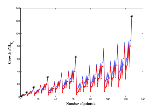
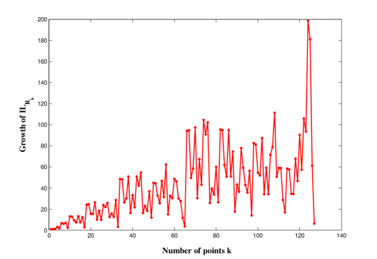
Figure 4.1: Exact Lebesgue constants associated to the $k$-sections of the Leja sequence $E$ and the assciated $\Re$-Leja sequence $R$ for $k=1,3,\dots,129$.

References

[1]L. Bialas-Ciez and J.P. Calvi,
Pseudo Leja sequences,
Ann. Mat. Pura Appl, (2012) 191, 53–75.
[2]S. Bernstein,
Sûr la limitation des valeurs d’un polynôme de
degré n sûr tout un segment par ses valeurs en points du
segment,
Isv. Akad. Nauk SSSR, 7 (1931), 1025–1050.
[3]J.P. Calvi and V.M. Phung,
On the Lebesgue constant of Leja sequences for the unit disk and its
applications to multivariate interpolation,
Journal of Approximation Theory 163-5, (2011), 608–622.
[4]J.P. Calvi and V.M. Phung,
Lagrange interpolation at real projections of Leja sequences for the unit disk,
Proceedings of the American Mathematical Society, 140(12): (2012), 4271–4284.
[5]A. Chkifa, A. Cohen, P.Y Passaggia and J PeterA comparative study between kriging and adaptive
sparse tensor-product methods for multi-dimensional
approximation problems in aerodynamics design
ESAIM: Proc. 48 (2015) 248–261.
[6]M.A. Chkifa,
On the Lebesgue constant of Leja sequences for
the complex unit disk and of their real projection,
Journal of Approximation Theory 166, (2013), 176–200.
[7]A. Cohen and M.A. Chkifa,
On the stability of polynomial interpolation using hierarchical sampling.
To appear in “Sampling theory, a renaissance” (2015), Birkhaeuser.
[8]M.A. Chkifa,
Méthodes polynomiales parcimonieuses en grande dimension.
Application aux EDP Paramétriques, PhD thesis, Laboratoire Jacques Louis Lions, (2014).
[9]A. Chkifa, A. Cohen and C. Schwab,
High-dimensional adaptive sparse polynomial interpolation
and applications to parametric PDEs,
Foundations of Computational Mathematic, (2013) 1–33.
[10]H.J. Bungartz and M. Griebel,
Sparse grids,
Acta Numerica13,(2004) 147–269.
[11]M.D. Gunzburger, C.G. Webster and Z. Guannan,
Stochastic finite element methods for partial
differential equations with random input data,
Acta Numerica23, (2014) 521–650
[12]Ph.J. Davis,
Interpolation and Approximation,
Blaisdell Publishing Company, (1963).
[13]V.K. Dzjadyk and V.V. Ivanov,
On asymptotics and estimates for the uniform norms of the
Lagrange interpolation polynomials corresponding to the Chebyshev
nodal points,
Analysis Mathematica, (1983) 9-11, 85–97.
[14]A. Irigoyen,
A uniform bound for the Lagrange polynomials
of Leja points for the unit disk
http://arxiv.org/pdf/1411.5527.pdf.
[15]R.A Devore and G.G Lorentz,
Constructive approximation,(1993), Springer.