Detection of Periodicity Based on Serial Dependence of Phase-Folded Data

Abstract

We introduce and test several novel approaches for periodicity detection in unevenly-spaced sparse datasets. Specifically, we examine five different kinds of periodicity metrics, which are based on non-parametric measures of serial dependence of the phase-folded data. We test the metrics through simulations in which we assess their performance in various situations, including various periodic signal shapes, different numbers of data points and different signal to noise ratios. One of the periodicity metrics we introduce seems to perform significantly better than the classical ones in some settings of interest to astronomers. We suggest that this periodicity metric – the Hoeffding-test periodicity metric – should be used in addition to the traditional methods, to increase periodicity detection probability.

1 Introduction

Detecting periodicity in an unevenly-sampled time series is a task one frequently faces in many fields of astronomy. Astronomers who study variable star light curves are probably the ones who face this challenge most often, but it is also common in the analysis of radial velocities (RV) of spectroscopic binary stars. The field of time-domain astronomy is becoming increasingly important. Large Time-domain surveys are already running (e.g. PTF (Law et al., 2009), CRTF (Drake et al., 2012), Pan-STARRS (Kaiser et al., 2010)) or planned (e.g. LSST (LSST Science Collaboration, 2009)), and some space-based astronomical missions are basically time-domain surveys (e.g. Kepler (Koch et al., 2010), CoRoT (Auvergne et al., 2009), Hipparcos (ESA, 1997), Gaia (Jordan, 2008)). The data analysis challenges that accompany the emerging huge databases emphasize the importance of periodicity detection in unevenly-sampled time series.

During the years many researchers proposed methods and algorithms to tackle the problem. A common approach is to calculate some kind of a periodicity metric function, which provides a periodicity score for each trial period. Period detection then consists of identifying a peak in the periodicity metric function that is significantly higher than all the other values. Depending on the specific kind of metric, one may sometimes look for a trough instead of a peak. In any case, the value of the periodicity score should be extreme at the correct value of the period, compared to its value at other periods.

An inherent difficulty in periodicity analysis of astronomical time series is the uneven time sampling. In classical time series analysis, Fourier techniques are available that decompose the original signal into a superposition of sinusoids. This approach is based on the orthogonality properties of evenly-sampled sinusoids. This cannot be done when the data are unevenly sampled, which is the common case in astronomy, since the sinusoids are no longer orthogonal.

Some methods devised for the unevenly-sampled case try to fit to the data some kind of a periodic function. The periodicity score is usually related in one way or another to the $\chi^{2}$ statistic of the fit. This is the ’least-squares’ group of techniques. The techniques in this group differ by the details of the periodic function and the exact calculation of the periodicity score. The most commonly used technique in this group is the Lomb–Scargle periodogram (Lomb, 1976; Scargle, 1982). Inspired by Fourier analysis, in Lomb–Scargle periodogram one fits a sinusoid to the time series. Another least-squares technique is the AoV method, which basically fits a periodic piecewise constant function (Schwarzenberg-Czerny, 1989). Other techniques exist that are based on the same general idea. Those methods are very powerful if the actual shape of the periodic signal is indeed close to the function the method assumes.

Another group of techniques is the ’string-length’ group. The classical methods in this group measure the sum of the squares of the differences between one data point and the next, after the points have been ordered in phase for a given trial period. Clarke (2002) provides an overview of the string-length techniques, focusing on the Lafler–Kinman method (Lafler & Kinman, 1965), and the methods of Renson (1978) and Dworetsky (1983). In all the string-length methods, one has to actually phase-fold the measurements for each trial period, and then quantify the serial dependence of the measurements, i.e., the dependence between consecutive measurements. The various string-length statistics used in those methods can all be traced back to the von-Neumann ratio statistic, also known as the Abbe value, or the Durbin–Watson statistic, which was used originally to detect autocorrelation in lag one in evenly-sampled time series (von Neumann et al., 1941; Durbin & Watson, 1950, 1951):

$$\eta=\frac{\sum(x_{i+1}-x_{i})^{2}}{\sum x_{i}^{2}}$$ (1)

The advantage of string-length techniques is obvious when we do not know in advance the shape of the periodic function we seek. The underlying assumption is that phase-folding the data at the correct period will produce a signal with some regularity, which will reflect as serial dependence of the data points.

In the current paper, we propose to take the string-length philosophy one step further and examine various non-parametric tests for serial dependence between consecutive phase-folded measurements. Although the term ’non-parametric’ is used extensively in statistics, its definition remains somewhat blurred. The basic idea is using as few assumptions as possible about the probability distribution of the quantity we study. A common feature to many non-parametric statistical techniques is the use of the order (or ’ranks’) of the data instead of their actual values (e.g. Lehmann, 1998). The use of ranks instead of the actual values can sometimes lead to surprisingly powerful results, in spite of the relative simplicity of the calculation and the obviously reduced information. Our hope is that this approach will be appropriate in cases where we are not sure of either the underlying periodic function or the statistical distribution of the noise.

We suggest to approach the problem of period detection through the notion of ’randomness tests’. When we do not phase-fold the data or phase-fold it in a wrong period, the data points are expected to behave randomly, whereas the correct phase-folding should reduce this randomness. Quantifying randomness is an important problem in the field of cryptography, which is concerned, among other things, with deterministically producing sequences that should exhibit randomness qualities. Thus, cryptography literature is rich in statistical tests, parametric and non-parametric, to test for randomness (e.g. Rukhin, 2001). Some of the tests we present here are also used in cryptography for this end.

Astronomical surveys have different characteristics, with respect to their noise distribution, sampling cadence, and size. In the current paper we compare the performance of the various techniques we introduce, when applying them to time series that contain a few dozen points, with an uneven sampling law. Basically, the performance tests we applied assume a survey with sampling characteristics that are very roughly similar to Hipparcos (ESA, 1997) or Gaia (Jordan, 2008), only in terms of their size and mean cadence. Since the data have to be phase-folded for every trial period, time series longer than a few thousand points, like the light curves of CoRoT (Auvergne et al., 2009) or Kepler (Koch et al., 2010), would probably require immense computing power and might lose their practicality.

It is important to mention that there have already been several attempts to apply the non-parametric approach to the problem of period detection in astronomical time series. However, the previous works use a somewhat different tool of non-parametric statistics – non-parametric regression. Those works attempt not only to estimate the period, but also the shape of the periodic function, under minimal assumptions, e.g. using Gaussian Kernels. Such are the works by Hall, Riemann & Rice (2000), Hall & Li (2006) and Wang, Khardon & Protopapas (2012). Recently, Sun, Hart & Genton (2012) proposed another non-parametric approach to period estimation, but it heavily relied on even sampling. Those studies emphasize the performance of their respective proposed methods in terms of estimated period accuracy. In our case, since we focus on sparsely sampled time series, we do not aim at the best achievable period accuracy, but at the ability to merely detect the periodicity with as few data points as possible. Such detection could trigger follow-up observations that would augment the sparse data to allow a more accurate period determination.

In the next section we introduce the non-parametric approaches that are the topic of this work. Later, in Section 3 we detail the suite of simulations and tests we used to perform the benchmark experiment. We discuss the results and offer some more insights in the last section.

2 Non-Parametric Measures of Serial Dependence

After a scan of the literature about non-parametric statistics, we chose five non-parametric methods to quantify the dependence between two variates. In fact the literature contains much more methods but we focused on five which we could tell were really independent.

Assuming there are $N$ data points, let us denote the phase-folded data by $x_{i}$ ($i=1,...,N$) where the index $i$ denotes the order after the phase folding. A serial dependence measure will test the dependence of the bivariate sample that consists of the pairs:

$$(x_{1},x_{2}),(x_{2},x_{3}),...,(x_{N-1},x_{N}),(x_{N},x_{1})\ .$$ (2)

Note the cyclic wraparound with the pair $(x_{N},x_{1})$. Some of the non-parametric methods use the rank statistics, where each value is replaced by its rank $R_{i}$, i.e., its place in the sorted sequence of values. For example, the sequence:

$$x_{i}=2.3,5.4,3.2,5.5,5.6,-3.2,0,19.4,1.2,40$$ (3)

will yield the rank sequence:

$$R_{i}=4,6,5,7,8,1,2,9,3,10$$ (4)

Other methods go further in reducing the information by replacing the value $x_{i}$ by a flag $F_{i}$ that signifies whether the actual value is above or below the median of the sample. In the example above, the flag sequence will read:

$$F_{i}=0,1,0,1,1,0,0,1,0,1$$ (5)

The literature suggests various special ways to deal with cases of ties or of odd sample size (where the median is actually one of the values). Furthermore, it should be emphasized that all the appearances in the literature of the tests we mention here are used originally as general dependence tests, not meant specifically for period detection. Thus, the original formulation of the tests uses no cyclic wraparound.

2.1 Bartels test

Robert Bartels introduced this test in 1982 as a rank version of the von Neumann’s ratio test (Bartels, 1982). In our case the expression for computing Bartels’ statistic is:

$$\beta=\sum_{i=1}^{N-1}(R_{i}-R_{i+1})^{2}+(R_{N}-R_{1})^{2}$$ (6)

One may say that this statistic is essentially a string-length statistic calculated for the ranks rather than for the actual values, and indeed this is the way Bartels described it.

In the same way that von Neumann’s ratio can be linearly related to the serial correlation coefficient, Bartels’ expression can be linearly related to the serial Spearman’s rank correlation coefficient (Spearman, 1904), and thus they are essentially equivalent. Note that in this current formulation, similarly to the von-Neumann ratio statistic, we expect a periodicity metric based on the Bartels statistic to exhibit a trough rather than a peak at the correct period.

2.2 Kendall’s tau ($\tau$)

Maurice Kendall introduced this test in 1938 (Kendall, 1938), as a measure of rank correlation. The calculation of Kendall’s $\tau$ is rather cumbersome. In order to calculate $\tau$ one goes over all $\frac{1}{2}N(N-1)$ pairs of ordered pairs of data points, i.e., pairs of the form $\left((x_{i},x_{i+1}),(x_{j},x_{j+1})\right)$. Of course, we assume that the ordered pairs include the pair $(x_{N},x_{1})$, in order to treat correctly the wraparound. A pair is said to be concordant if the ranks for both elements agree, i.e., if both $x_{i}>x_{i+1}$ and $x_{j}>x_{j+1}$, or if both $x_{i}<x_{i+1}$ and $x_{j}<x_{j+1}$. Otherwise it is said to be discordant. Denote by $N_{c}$ the number of concordant pairs and by $N_{d}$ the number of discordant pairs. Kendall’s $\tau$ is then defined by:

$$\tau=\frac{N_{c}-N_{d}}{\frac{1}{2}N(N-1)}\ .$$ (7)

Kendall’s $\tau$ is non-parametric in the sense that the actual values of the data are not relevant, only their order.

2.3 Runs test

The runs test procedure counts the number of runs of constant flags $F_{i}$, or equivalently, the number of times the flags change. Recall that the flag $F_{i}$ equals zero if the original value is below the median, and equals one otherwise. Thus, one may write an algebraic definition:

$$U=\sum_{i=1}^{N-1}|F_{i+1}-F_{i}|+|F_{1}-F_{N}|$$ (8)

Wald & Wolfowitz (1940) first introduced this test in a somewhat different context of testing whether two samples were drawn from the same population. In our case, obviously, runs are counted only for a single cycle. Note that at the correct period we expect the data points to get organized in as few runs as possible, so we expect the correct period to exhibit a trough in the periodicity metric plot rather than a peak (like in the Bartels-test or the von-Neumann-ratio cases).

2.4 Corner test

Olmstead & Tukey (1947) proposed the rather elaborate corner test for finding association between two variables, in situations where we suspect that information about association may concentrate in points on the periphery of the dataset. To effect the test, in the $xy$ scatter plot of the paired dataset, draw in the $x$ and $y$ median lines, and label the quadrants so formed $+$,$-$,$+$,$-$, serially from the top right-hand corner. Thus, in this new Cartesian coordinate system, the first and third quadrants are labeled positive, and the second and fourth negative. Then, starting at the top, move vertically down counting points with decreasing $y$ values until it is necessary to cross the $x$ median line, and attach to this count the sign of the quadrant in which the points lie. Proceed in similar fashion for the bottom, left- and right-hand sides of the dataset. The test statistic is then the sum of the four counts with their signs. Olmstead & Tukey (1947) provide an example for the calculation, together with a graphic visualization, and suggest a treatment for ties.

2.5 Hoeffding test

In 1948, Wassily Hoeffding proposed an even more elaborate statistic than the corner test (Hoeffding, 1948). Hoeffding’s statistic is based on the population measure of the deviation of the bivariate distribution from independence. This statistic is especially suitable for quantifying general kinds of dependence, not necessarily linear or even monotone. Adapted to our case including the wraparound points, Hoeffding’s statistic is computed as follows:

$$D=\frac{A-2(N-2)B+(N-2)(N-3)C}{N(N-1)(N-2)(N-3)(N-4)}$$ (9)

where

$$A=\sum_{i=1}^{N-1}(R_{i}-1)(R_{i}-2)(R_{i+1}-1)(R_{i+1}-2)+(R_{N}-1)(R_{N}-2)(R_{1}-1)(R_{1}-2)\ ,$$ (10)

$$B=\sum_{i=1}^{N-1}(R_{i}-2)(R_{i+1}-2)c_{i}+(R_{N}-2)(R_{1}-2)c_{N}\ ,$$ (11)

$$C=\sum_{i=1}^{N}c_{i}(c_{i}-1).$$ (12)

where $c_{i}$ (sometimes called the bivariate rank) is the number of pairs $(x_{j},x_{j+1})$ for which both $x_{j}<x_{i}$ and $x_{j+1}<x_{i+1}$.

3 Simulations

We present here a suite of simulations we have performed in order to assess the competitiveness of the tests introduced in the previous section against the traditional methods of least squares and string length.

3.1 Simulated signals

In all the simulations we present here, we randomly drew a sparse set of sampling times, from a total time baseline spanning $1000$ time units (for convenience, we henceforth denote our arbitrary time unit by ’days’, referring to the intended applications in astronomy). We then used those times to sample a periodic function (see below) and added white Gaussian noise, whose amplitude we determined based on a prescribed signal to noise ratio (SNR). The SNR here means the ratio between the standard deviation of the specific simulated data points without the noise, and the standard deviation of the Gaussian noise. In the simulations we present here we simulated a periodic function with a period of two days. We checked with a few simulations that the results did not change in any significant manner when we tried other periods.

The simulations are intended to be very generic. We wished to test the case of an unevenly sampled sparse dataset, i.e. with not many samples. We therefore used the most generic non-uniform sampling – random times drawn from a uniform distribution. We thus have not included any sampling biases one might encounter in astronomy. We also used the most generic form of noise – noise drawn from a Gaussian distribution. When the techniques we present here are implemented in specific astronomical cases, it will be important to test them in the specific context.

The different shapes of periodic functions we used, ranged from purely sinusoidal shape to extremely non-sinusoidal. The shapes and the formulae we used to produce them are detailed below, as a function of the phase ${\phi=\frac{t\mod{P}}{P}}$ :

A.

Pure sinusoidal function:

$$x=\cos(2\pi\phi)$$ (13)

B.

Mildly non-sinusoidal function (’almost sinusoidal’) :

$$x=\cos(2\pi\phi)+0.25\cos(4\pi\phi)$$ (14)

C.

Sawtooth wave:

$$x=\phi$$ (15)

D.

Pulse wave. In the simulations we have used a pulse wave with pulse duration of two thirds of the period:

$$x=\begin{cases}0&\text{if $\phi<1/3$},\\ 1&\text{otherwise}.\end{cases}$$ (16)

E.

Eclipsing binary light curve. We approximated the lightcurve of an eccentric eclipsing binary by subtracting two Gaussian functions from a constant baseline of $1$. The first Gaussian was centred around phase $0.0$, with a maximum value of $0.5$, and the second one centred around phase $0.4$, with a maximum value of $0.2$.

F.

Spectroscopic binary radial velocity (RV) curve. Using the well-known formulae for spectroscopic binary RV, we simulated a RV curve with an eccentricity of $0.97$ and an argument of periastron $\omega=\frac{\pi}{4}$.

The exact amplitudes and offset values of the above detailed functions do not matter for our purposes, only the SNR of the various cases we simulated. Fig. 1 portrays schematically the six shapes.

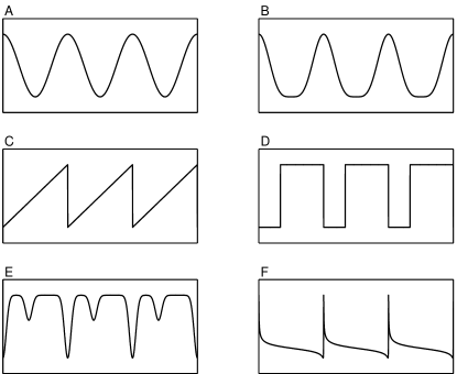
Figure 1: A Schematic illustration of the six periodic functions used in the simulations. A. Sinusoidal; B. Almost sinusoidal; C. Sawtooth; D. Pulse wave; E. Eclipsing binary light curve; F. Eccentric spectroscopic binary RV curve. For detailed descriptions of the various shapes see text.

3.2 Examples

Figs 2–7 show the results of applying all the methods on simulated periodic time series with $100$ data points, and SNR of $100$. This is a relatively easy task, and in almost all cases, the correct peak is retrieved, except for the case of the Lomb–Scargle periodogram applied to the eclipsing binary case. In this specific case, the Lomb–Scargle periodogram has a prominent peak in the second harmonic of the true frequency (at a frequency of $1\,\mathrm{d}^{-1}$), instead of the correct one. The peak in the correct period is much lower than this second harmonic. This is a well known feature of the Lomb–Scargle periodogram, and it usually does not constitute a problem, since the peak at the second harmonic already leads to a detection, and further scrutiny of the light curve reveals the correct period. One can also clearly see the appearance of sub-harmonic peaks at almost all periodicity metric plots, besides Lomb–Scargle periodogram. Judging subjectively only by these specific idealized examples, we can say that besides the case of the pulse-wave periodicity, the Hoeffding-test periodicity metric provides the ’cleanest’ detection: a clear peak at the correct period, with very low variability in other periods (potentially implying a very small chance of false detection), except for the subharmonics.

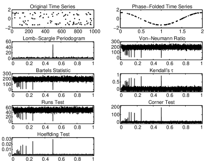
Figure 2: The results of applying all the examined periodicity detection methods to a simulated time-series, of the sinusoidal type, with $100$ simulated data points, and a SNR of $100$. The upper two panels show the time series and its phase-folded version, using the correct period. The other panels show the periodicity metrics calculated for this time series, with self explanatory titles.

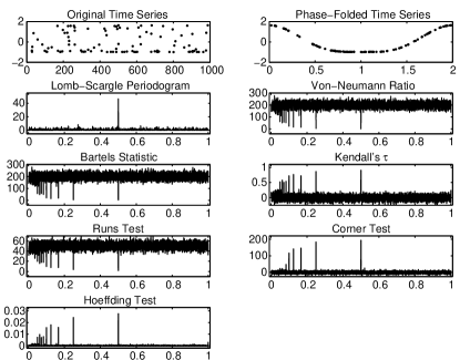
Figure 3: The results of applying all the examined periodicity detection methods to a simulated time-series, of the ’almost sinusoidal’ type, with $100$ simulated data points, and a SNR of $100$. The upper two panels show the time series and its phase-folded version, using the correct period. The other panels show the periodicity metrics calculated for this time series, with self explanatory titles.

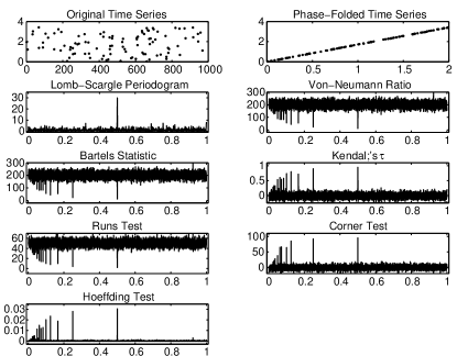
Figure 4: The results of applying all the examined periodicity detection methods to a simulated time-series, of the sawtooth type, with $100$ simulated data points, and a SNR of $100$. The upper two panels show the time series and its phase-folded version, using the correct period. The other panels show the periodicity metrics calculated for this time series, with self explanatory titles.

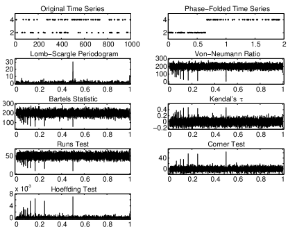
Figure 5: The results of applying all the examined periodicity detection methods to a simulated time-series, of the pulse wave type, with $100$ simulated data points, and a SNR of $100$. The upper two panels show the time series and its phase-folded version, using the correct period. The other panels show the periodicity metrics calculated for this time series, with self explanatory titles.

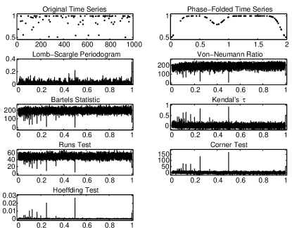
Figure 6: The results of applying all the examined periodicity detection methods to a simulated time-series, of the eclipsing binary lightcurve type, with $100$ simulated data points, and a SNR of $100$. The upper two panels show the time series and its phase-folded version, using the correct period. The other panels show the periodicity metrics calculated for this time series, with self explanatory titles.

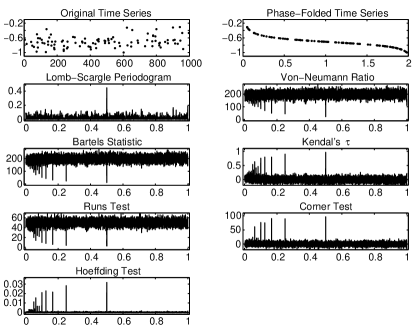
Figure 7: The results of applying all the examined periodicity detection methods to a simulated time-series, of the spectroscopic binary RV curve type, with $100$ simulated data points, and a SNR of $100$. The upper two panels show the time series and its phase-folded version, using the correct period. The other panels show the periodicity metrics calculated for this time series, with self explanatory titles.

Figs 8–13 present tougher cases – time series with $30$ data points, and SNR of $3$. This time, as one would expect, the results are not as impressive as in the cases with more points and higher SNR. In the sinusoidal and almost-sinusoidal cases it seems that all metrics still exhibit the correct peak, but it is much less prominent against the background of the other periods. The Hoeffding-test metric still competes very well with the Lomb–Scargle periodogram, and seems to be much more conclusive compared to the other methods. In the sawtooth and the spectroscopic binary case the superiority of the Hoeffding-test metric over all the others, including the Lomb–Scargle periodogram, is evident. In the pulse-wave and the eclipsing binary cases all methods perform poorly, with a minor preference for Lomb–Scargle over the Hoeffding test.

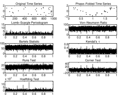
Figure 8: The results of applying all the examined periodicity detection methods to a simulated time-series, of the sinusoidal type, with $30$ simulated data points, and a SNR of $3$. The upper two panels show the time series and its phase-folded version, using the correct period. The other panels show the periodicity metrics calculated for this time series, with self explanatory titles.

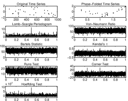
Figure 9: The results of applying all the examined periodicity detection methods to a simulated time-series, of the ’almost sinusoidal’ type, with $30$ simulated data points, and a SNR of $3$. The upper two panels show the time series and its phase-folded version, using the correct period. The other panels show the periodicity metrics calculated for this time series, with self explanatory titles.

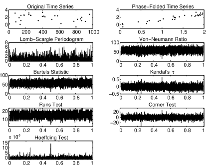
Figure 10: The results of applying all the examined periodicity detection methods to a simulated time-series, of the sawtooth type, with $30$ simulated data points, and a SNR of $3$. The upper two panels show the time series and its phase-folded version, using the correct period. The other panels show the periodicity metrics calculated for this time series, with self explanatory titles.

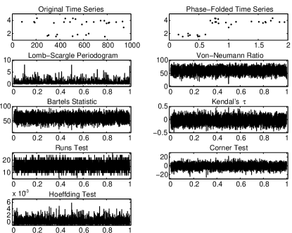
Figure 11: The results of applying all the examined periodicity detection methods to a simulated time-series, of the pulse wave type, with $30$ simulated data points, and a SNR of $3$. The upper two panels show the time series and its phase-folded version, using the correct period. The other panels show the periodicity metrics calculated for this time series, with self explanatory titles.

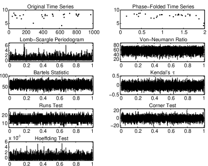
Figure 12: The results of applying all the examined periodicity detection methods to a simulated time-series, of the eclipsing binary light curve type, with $30$ simulated data points, and a SNR of $3$. The upper two panels show the time series and its phase-folded version, using the correct period. The other panels show the periodicity metrics calculated for this time series, with self explanatory titles.

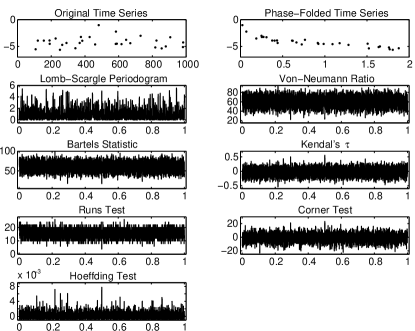
Figure 13: The results of applying all the examined periodicity detection methods to a simulated time-series, of the spectroscopic binary RV curve type, with $30$ simulated data points, and a SNR of $3$. The upper two panels show the time series and its phase-folded version, using the correct period. The other panels show the periodicity metrics calculated for this time series, with self explanatory titles.

3.3 Performance testing

For each simulated time series we calculated the five periodicity metric functions we introduced earlier. As a base for comparison we also calculated the classical Lomb–Scargle periodogram, and also the von-Neumann ratio periodicity metric, as representatives of the more traditional methods.

We calculated the periodicity metric functions for a grid of frequencies, ranging from $10^{-4}$ to $1\,\mathrm{d}^{-1}$, with steps of $10^{-4}\,\mathrm{d}^{-1}$. Thus, the simulated period of two days is located at the middle of the frequency range we used, at a frequency of $0.5\,\mathrm{d}^{-1}$.

Knowing the true period, we used as a performance metric for our benchmark experiment, the degree to which the periodicity score statistic at the correct period can be singled out compared to the values at other periods. This should be made cautiously, since the null-hypothesis distribution is different for each statistic. In order to overcome this hurdle we prepared for each statistic a reference sample of random datasets (pure noise, no signal) of the same number of points as the one being tested. The size of the reference sample was $10^{6}$. Each value in the tested method was converted using quantiles of this empirical reference distribution. In order to transform extreme values, that were not obtained in the random $10^{6}$ reference samples, we extrapolated the distribution using a maximum-likelihood fit of a generalized Pareto distribution that was applied to the $10^{-3}$ distribution tail (e.g. de Zea Bermudez & Kotz, 2010). Our experience showed that robustness required to exclude the $10$ most extreme values of the sample, while constraining the Pareto distribution shape parameter to be non-positive (de Zea Bermudez & Kotz, 2010). Generalized Pareto distribution was not suitable for the runs-test distribution tail, but a Gaussian approximation seemed to be a good-enough approximation (in the same way it is used as an approximation to the binomial distribution).

After the conversion based on the reference distribution, we measured the difference between the value at the correct period and the average value of the statistic , and normalized it by the standard deviation of the statistic on all periods. Following Kovács, Zucker & Mazeh (2002) and Alcock et al. (2000), we called this quantity SDE (Signal Detection Efficiency):

$$\mathrm{SDE}=\frac{S(f_{0})-\bar{S}}{\mathrm{SD}(S)}$$ (17)

where $S$ is the tested periodicity metric function, $f_{0}$ is the true frequency, and $\bar{S}$ and $\mathrm{SD}(S)$ are the mean and standard deviation of the function. Note that our SDE is a little different from the SDE in the papers by Kovács et al. (2002) and Alcock et al. (2000), where they use the peak value of the function, and not the value at the known period. Our version of the SDE tests specifically the ability of the tested method to single out the correct period, which is known in advance in a simulation context.

3.4 Performance trends

In Fig. 14 we present the results of performing $100$ time series simulations with $100$ points each, and varying SNRs, for each of the periodic functions. The values we plot in the figure are the SDE, computed as we described above, after the conversion using the reference distribution, averaged over the $100$ trials in every configuration. In almost all situations the Hoeffding-test method outperforms all other methods tested. The only situation where it seems that the Lomb–Scargle consistently outperforms the Hoeffding-test method is the case of the pulse-wave periodic function. This was evident already in the examples (Fig. 5). Probably the piecewise constant nature of the signal makes ranking information irrelevant, whereas ranking has no effect on the least-square fit. This also reflects in the fact that the performance of the non-parametric techniques hardly improves with increasing SNR for the pulse-wave case.

Based on the examples (Fig. 6), we can also understand how Lomb–Scargle performed so poorly in the eclipsing-binary cases. The correct period (the fundamental frequency) almost does not exhibit a peak in the periodogram, only the second harmonic does. The serial dependence of the phase-folded light curve still remains, which allows the non-parametric methods to perform the way they do in the other cases.

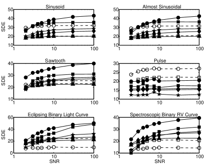
Figure 14: SDE as a function of SNR for $100$ points time series. The SDE is averaged over $100$ simulated light curves. Legend: empty circles, dashed line – Lomb–Scargle periodogram; empty squares, dashed line – von-Neumann Ratio; filled upward-pointing triangles, solid line – Bartels test; filled diamonds, solid line – Kendall’s tau; filled pentagrams, solid line – runs test; filled squares, solid line – corner test; filled circles, solid line – Hoeffding-test .

In Fig. 15 we present a more difficult case, where the number of data points is much smaller – $20$. This time the advantage of the traditional techniques in the pulse-wave case is even more pronounced. Some non-parametric techniques seem to be preferable over the classical ones in the higher SNRs, and the Hoeffding test maintains its superiority in most cases.

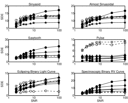
Figure 15: SDE as a function of SNR for $20$ points time series. The SDE is averaged over $100$ simulated light curves. Legend: empty circles, dashed line – Lomb–Scargle periodogram; empty squares, dashed line – von-Neumann Ratio; filled upward-pointing triangles, solid line – Bartels test; filled diamonds, solid line – Kendall’s tau; filled pentagrams, solid line – runs test; filled squares, solid line – corner test; filled circles, solid line – Hoeffding-test.

Fig. 16 examines the dependence of the SDE on the number of points in the time series. This time we held the SNR fixed at $100$ while we varied the number of data points. Again, the figure displays the averaged SDE over $100$ random realizations of the simulation. The superiority of the Hoeffding-test method is evident for all kinds of periodicities except for the pulse-wave, where the traditional methods keep on being superior .

Fig. 17 presents the same test for the case of SNR fixed at $3$. Again, the Hoeffding-test method is definitely superior for the sawtooth wave and the spectroscopic binary RV case, and it is competitive with the classical approaches in the other cases, except the pulse wave.

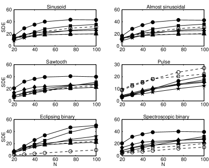
Figure 16: SDE as a function of the number of data points for time series with SNR of $100$. The SDE is averaged over $100$ simulated light curves. Legend: empty circles, dashed line – Lomb–Scargle periodogram; empty squares, dashed line – von-Neumann Ratio; filled upward-pointing triangles, solid line – Bartels test; filled diamonds, solid line – Kendall’s tau; filled pentagrams, solid line – runs test; filled squares, solid line – corner test; filled circles, solid line – Hoeffding-test.

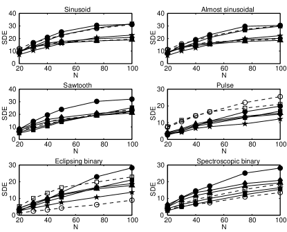
Figure 17: SDE as a function of the number of data points for time series with SNR of $3$. The SDE is averaged over $100$ simulated light curves. Legend: empty circles, dashed line – Lomb–Scargle periodogram; empty squares, dashed line – von-Neumann Ratio; filled upward-pointing triangles, solid line – Bartels test; filled diamonds, solid line – Kendall’s tau; filled pentagrams, solid line – runs test; filled squares, solid line – corner test; filled circles, solid line – Hoeffding-test.

We can summarize that unless there are significantly long constant intervals in the periodicity shape, the superiority of the Hoeffding-test method is most prominent in the extremely non-sinusoidal cases, which are obviously of interest in astronomy – the cases of the eclipsing binary light curve and the spectroscopic binary RV curve.

The SDE plots we presented above are of a statistical nature. One may still wonder whether those results have practical meaning. We therefore checked individually the spectroscopic binary RV simulations for the case of $30$ data points and SNR of $3$ to get an impression. According to Fig. 17, in this setting it seems there was a marked difference between the performance of the Hoeffding test and the classical methods. Indeed, it was quite easy to find cases where the Lomb–Scargle periodogram simply missed the detection while the Hoeffding-test method provided a clear detection (in fact, they were the majority). We present three such example in Figs 18–20. This is obviously not a statistical proof, just a demonstration of one aspect of the statistical study presented earlier.

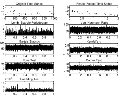
Figure 18: An example of the results of applying all the examined periodicity detection methods to a simulated time-series, of the spectroscopic binary RV curve type, with $30$ simulated data points, and a SNR of $3$. The upper two panels show the time series and its phase-folded version, using the correct period. The other panels show the periodicity metrics calculated for this time series, with self explanatory titles. Note the complete non-detection at the Lomb–Scargle periodogram and the von-Neumann ratio, and the very noticeable detection by the Hoeffding-test technique.

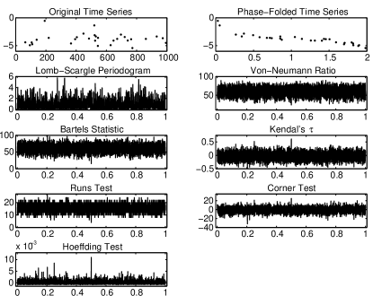
Figure 19: Another example of the results of applying all the examined periodicity detection methods to a simulated time-series, of the spectroscopic binary RV curve type, with $30$ simulated data points, and a SNR of $3$. The upper two panels show the time series and its phase-folded version, using the correct period. The other panels show the periodicity metrics calculated for this time series, with self explanatory titles. Note the complete non-detection at the Lomb–Scargle periodogram and the von-Neumann ratio, and the very noticeable detection by the Hoeffding-test technique.

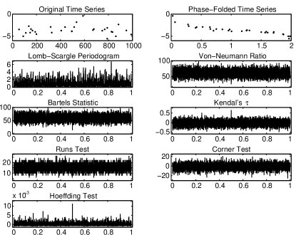
Figure 20: Another example of the results of applying all the examined periodicity detection methods to a simulated time-series, of the spectroscopic binary RV curve type, with $30$ simulated data points, and a SNR of $3$. The upper two panels show the time series and its phase-folded version, using the correct period. The other panels show the periodicity metrics calculated for this time series, with self explanatory titles. Note the complete non-detection at the Lomb–Scargle periodogram and the von-Neumann ratio, and the very noticeable detection by the Hoeffding-test technique.

4 Discussion

We have presented here several kinds of periodicity metric statistics based on non-parametric serial dependence measures, and assessed their performance. It turns out that one of those methods, the Hoeffding-test method, has the potential to be much more powerful than the traditional parametric approaches of Lomb–Scargle and string length for extremely non-sinusoidal periodicities.

The large time-domain surveys mentioned in the Introduction are bound to provide, besides the easily detectable periodicity shapes, also extreme cases with high harmonic content (non-sinusoidal). These may be either extreme cases of eclipsing binaries, or even periodicity shapes we are not aware of yet. In order to fully realize the exploratory potential of those surveys, it is important to increase the detection probability of the extreme cases. This is where the techniques presented here become essential.

There are several new directions for further research that are now open. Computationally, the calculation may be quite demanding, since it involves rearranging the data values all over again for each period (phase-folding). This operation, which is basically an operation of sorting, is of complexity $O(N\log N)$. Repeating this for every period may render the methods we introduced impractical for large datasets. This warrants some algorithmic research to look for fast techniques to perform the operation.

The very impressive results of the Hoeffding-test metric merit a closer look at its definition and the theory behind it. As a test of independence between two random variables, it is based on the measure of deviation from independence of the two variables. Let us denote by $G_{1}$ and $G_{2}$ the cumulative distribution functions of the two variables, and by $G_{12}$ their joint cumulative distribution function. Then, independence of the two variables would mean $G_{12}=G_{1}G_{2}$. Armed with this definition, and using Cramér–von Mises criterion for distance between distributions (Cramér, 1928; von Mises, 1928), Hoeffding defined $D$ by:

$$\int(G_{12}-G_{1}G_{2})^{2}\,dG_{12}\ ,$$

where we use the empirical distribution function, determined only by the observed values. This is somewhat reminiscent of the Kolmogorov–Smirnov philosophy, which is popular among astronomers (e.g. Babu & Feigelson, 2006). This formula eventually results in the formulae presented in Eqs 9–12.

It is now clear why Hoeffding test tests for any kind of dependence, not necessarily linear or even monotonous. Fig. 21 provides further insight. For each periodic signal shape We simulated $200$ light curves with $100$ points each, and with SNR $5$. We then plotted the dependence between each sample and its successor, after phase folding. In the simpler cases of sinusoidal and almost-sinusoidal (panels A,B), the dependence seems completely linear. This explains the satisfactory performance of von_Neumann ratio in these cases. In the other panels the departure from linearity may be quite significant, especially in the sawtooth and eccentric binary RV cases. A strong departure from linearity is also apparent in the pulse-shape periodicity, but one has to remember that the plot seems very similar when folding in the wrong period, which explains why the periodicity metric peak in those cases is not very prominent.

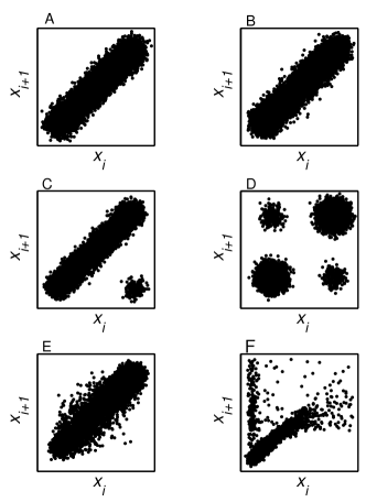
Figure 21: The dependence between consecutive phase-folded samples for each periodic-signal shape examined. The specific panels correspond to the panels in Fig. 1: A. Sinusoidal; B. Almost sinusoidal; C. Sawtooth; D. Pulse wave; E. Eclipsing binary light curve; F. Eccentric spectroscopic binary RV curve.

We also note here that we use the original expression that Hoeffding introduced. At a later stage, Blum, Kiefer & Rosenblatt (1961) proposed an approximation to the Hoeffding statistic that is much easier to compute, and in the context of periodicity detection it may open possibilities for further simplifications. Hoeffding did not provide any intuitive meaning to the various quantities used in the calculation – $A$, $B$, and $C$ (Eqs 10–12). The only one which seems to have an obvious meaning is $A$ (Eq. 10), which is a measure of the serial correlation of the squared ranks.

In terms of the statistic used, recall that our rationale is based on the rationale of the string-length methods. Besides pure serial dependence measures, several authors tried to incorporate into the string-length statistics also information related to the actual phase of the measurements, penalizing pairs of consecutive points with large phase difference (e.g. Burke, Rollland & Boy, 1970; Renson, 1978). This may be attempted also in any one of the techniques we surveyed here, and perhaps it may improve the performance even more.

In the simulations we present we use a completely random time sampling, representing completely uneven sampling. In real-life astronomical applications time sampling can have a quasi-periodic nature, especially related to day-night alternation, but also to lunar phase (monthly) and observability of the studied object (annual). This is also true in a more complicated way for the cases of Gaia and Hipparcos. This may somehow affect the simulation results, probably by introducing aliases. However, since this paper is only the first introduction of the new methods, we have not gone into the details of exploring the full range of astronomical contexts.

Another idealization we have made in this work is considering only white noise, with a prescribed SNR. Life is obviously more complex than that, and in real-life signals there are also trends and systematics (’red noise’). An obvious way to deal with those is by applying a preliminary stage of detrending. Nevertheless, it would be interesting to test the robustness of the non-parametric techniques against such phenomena. A similar problem is the problem of multi-periodic signals, which are also a problem for the conventional string-length methods. As real-life tests, one should also test the techniques on existing sparsely sampled databases, e.g., Hipparcos Epoch Photometry (ESA, 1997), and see whether we detect all the known periodicities, and maybe add some more unknown ones.

We focused here on tests of serial dependence of the phase-folded data. However, there are many other tests of non-parametric statistics, and there is potential for more innovative ways to turn them into periodicity metrics.

While we introduce here five new kinds of periodicity metrics, it seems that one of them – the serial Hoeffding-test statistic – emerges as a very promising new periodicity detection method, that may improve periodicity detection significantly. As part of its ’maturation’ process, it should be further studied, both in terms of the period detection efficiency and in terms of the estimation accuracy, in various configurations. To promote further research and testing of this periodicity metric we make it available online, in the form of a Matlab function.

References

- Alcock et al. (2000) Alcock C. et al. 2000, ApJ, 542, 257
- Auvergne et al. (2009) Auvergne M. et al. 2009, A&A, 506, 411
- Babu & Feigelson (2006) Babu G. J., Feigelson, E. D. 2006 in Gabriel C., Arviset, C., Ponz D., Enrique S., eds, ASP Conf. Ser. Vol. 351, Astronomical Data Analysis Software and Systems XV. Astron. Soc. Pac., San Francisco, p. 127
- Bartels (1982) Bartels R. 1982, J. Am. Stat. Assoc., 77, 40
- Blum et al. (1961) Blum J. R., Kiefer J., Rosenblatt M. 1961, Ann. Math. Stat., 32, 485
- Burke et al. (1970) Burke E. W., Rolland W. W., Boy W. R. 1970, J. Roy. Astron. Soc. Can., 64, 353
- Clarke (2002) Clarke D. 2002, A&A, 386, 763
- Cramér (1928) Cramér H. 1928, Scand. Actuar. J., 11, 13
- de Zea Bermudez & Kotz (2010) de Zea Bermudez P., Kotz S. 2010, J. Stat. Plan. Infer., 140, 1353
- Drake et al. (2012) Drake A. J. et al. 2012, in Griffin E., Hanisch R., Seaman R., eds, IAU Symp. 285, New Horizons in Time-Domain Astronomy. Cambridge Univ. Press, Cambridge, p. 306
- Durbin & Watson (1950) Durbin J., Watson G. S. 1950, Biometrika, 37, 409
- Durbin & Watson (1951) Durbin J., Watson G. S. 1951, Biometrika, 38, 159
- Dworetsky (1983) Dworetsky M. M. 1983, MNRAS, 203, 917
- ESA (1997) ESA 1997, The Hipparcos and Tycho Catalogues, ESA SP-1200
- Hall & Li (2006) Hall P., Li M. 2006, Biometrika, 93, 411
- Hall et al. (2000) Hall P., Riemann J., Rice J. 2000, Biometrika, 87, 545
- Hoeffding (1948) Hoeffding W. 1948, Ann. Math. Stat., 19, 293
- Jordan (2008) Jordan S. 2008, Astron. Nachr., 329, 875
- Kaiser et al. (2010) Kaiser, N. et al. 2010, Proc. SPIE, 7733, 77330E
- Kendall (1938) Kendall M. G. 1938, Biometrika, 30, 81
- Koch et al. (2010) Koch D. G. et al. 2010, ApJ, 713, L79
- Kovács et al. (2002) Kovács G., Zucker S., Mazeh T. 2002, A&A, 391, 369
- Lafler & Kinman (1965) Lafler J., & Kinman, T. D. 1965, ApJS, 11, 216
- Law et al. (2009) Law N. M. et al. 2009, PASP, 121, 1395
- Lehmann (1998) Lehmann E. L. 1998, Nonparametrics: Statistical Methods Based on Ranks. Prentice Hall, Upper Saddle River, NJ
- Lomb (1976) Lomb N. R. 1976, Ap&SS, 39, 447
- LSST Science Collaboration (2009) LSST Science Collaboration 2009, preprint (arXiv: 0912.0201)
- Olmstead & Tukey (1947) Olmstead P. S., Tukey J. W. 1947, Ann. Math. Stat., 18, 495
- Renson (1978) Renson P. 1978, A&A, 63, 125
- Rukhin (2001) Rukhin A. L. 2001, Theory Probab. Appl., 45, 111
- Scargle (1982) Scargle J. D. 1982, ApJ, 263, 835
- Schwarzenberg-Czerny (1989) Schwarzenberg-Czerny A. 1989, MNRAS, 241, 153
- Spearman (1904) Spearman C. 1904, Amer. J. Psycho., 15, 72
- Sun et al. (2012) Sun Y., Hart J. D., Genton M. G. 2002, Technometrics, 54, 83
- von Mises (1928) von Mises R. 1928, Wahrscheinlichkeit, Statistik und Wahrheit. Julius Springer, Vienna
- von Neumann et al. (1941) von Neumann J., Kent R. H., Bellinson H. R., Hart B. I. 1941, Ann. Math. Stat., 12, 153
- Wald & Wolfowitz (1940) Wald A., Wolfowitz J. 1940, Ann. Math. Stat., 11, 147
- Wang et al. (2012) Wang Y., Khardon R., Protopapas, P. 2012, ApJ, 756, 67