Min-Max Kernels

Abstract

The min-max kernel is a generalization of the popular resemblance kernel (which is designed for binary data). In this paper, we demonstrate, through an extensive classification study using kernel machines, that the min-max kernel often provides an effective measure of similarity for nonnegative data. As the min-max kernel is nonlinear and might be difficult to be used for industrial applications with massive data, we show that the min-max kernel can be linearized via hashing techniques. This allows practitioners to apply min-max kernel to large-scale applications using well matured linear algorithms such as linear SVM or logistic regression.

The previous remarkable work on consistent weighted sampling (CWS) produces samples in the form of ($i^{*},t^{*}$) where the $i^{*}$ records the location (and in fact also the weights) information analogous to the samples produced by classical minwise hashing on binary data. Because the $t^{*}$ is theoretically unbounded, it was not immediately clear how to effectively implement CWS for building large-scale linear classifiers. In this paper, we provide a simple solution by discarding $t^{*}$ (which we refer to as the “0-bit” scheme). Via an extensive empirical study, we show that this 0-bit scheme does not lose essential information. We then apply the “0-bit” CWS for building linear classifiers to approximate min-max kernel classifiers, as extensively validated on a wide range of publicly available classification datasets.

We expect this work will generate interests among data mining practitioners who would like to efficiently utilize the nonlinear information of non-binary and nonnegative data.

1 Introduction

Nonnegative data are common in practice and the existence of negative entries in a dataset is often due to shifting or normalization. In this paper we show that the min-max kernel can provide an effective measure of similarity for nonnegative data and should be useful for building effective large-scale data mining tools via hashing techniques.

Given two nonnegative data vectors, $u,v\in\mathbb{R}^{D}$, we define

$$\textbf{min-max}:\hskip 7.22743ptK_{MM}(u,v)=\frac{\sum_{i=1}^{D}\min\{u_{i},\ v_{i}\}}{\sum_{i=1}^{D}\max\{u_{i},\ v_{i}\}}$$ (1)

which is a generalization of the well-known resemblance:

$$\textbf{resemblance}:K_{R}(u,v)=\frac{\sum_{i=1}^{D}1\{u_{i}>0\text{ and }v_{i}>0\}}{\sum_{i=1}^{D}1\{u_{i}>0\text{ or }v_{i}>0\}}$$ (2)

The resemblance is a popular measure of similarity for binary data [4, 20]. The prior work [22] used the term “resemblance kernel” because the resemblance can be written as the (expectation) of an inner product (and hence it is a positive definite kernel). It will be soon clear that $K_{MM}$ (1) can also be written as the expectation of an inner product.

Readers (e.g., those from computer vision) probably have realized that the min-max kernel defined in (1) is related to the following so-called intersection kernel [23]:

$$\textbf{intersection}:\hskip 7.22743pt K_{I}(u,v)=\sum_{i=1}^{D}\min\{u_{i},\ v_{i}\},$$ (3)

$$\sum_{i=1}^{D}u_{i}=1,\ \ \ \sum_{i=1}^{D}v_{i}=1$$

In this paper, we will extensively compare the min-max kernel with the intersection kernel in the context of kernel machines for classification. Interestingly, for most datasets in our experimental study, the min-max kernel outperforms the intersection kernel, and in some cases significantly so. Of course, another advantage of the min-max kernel is the existence of hashing techniques [24, 14] to approximate this nonlinear kernel by linear kernel (at least conceptually).

The sum-to-one normalization in the definition of intersection kernel (3) appears natural, since the data vectors (e.g., $u$ and $v$) were treated as histograms when the intersection kernel was designed. For our curiosity, we also define, what we call, the “normalized min-max kernel” as follows:

$$\textbf{n-min-max}:\hskip 7.22743pt K_{NMM}(u,v)=\frac{\sum_{i=1}^{D}\min\{u_{i},\ v_{i}\}}{\sum_{i=1}^{D}\max\{u_{i},\ v_{i}\}}$$ (4)

$$\sum_{i=1}^{D}u_{i}=1,\ \ \ \sum_{i=1}^{D}v_{i}=1$$

Our experiments will show that, for most datasets, this normalization step only affects the classification accuracies very marginally, although there are also exceptions. In this paper, we often use “min-max kernels” to refer to both the min-max kernel and the n-min-max kernel. Note that the normalization step is conducted before applying hashing, which means that these two kernels are no different as far as the research on hashing is concerned.

It is worth mentioning that the above three kernels (min-max, intersection, and n-min-max) have no tuning parameters. Thus, it is often possible to further improve the performance by, for example, using multiple kernels or kernels combined in a special fashion (e.g., the CoRE kernels [19] by multiplying resemblance with correlation).

We will compare these three types of parameter-free kernels with the basic (tuning-free) kernel:

$$\textbf{linear}:\hskip 7.22743pt K_{\rho}(u,v)=\sum_{i=1}^{D}u_{i}v_{i},$$ (5)

$$\sum_{i=1}^{D}u_{i}^{2}=1,\ \ \ \sum_{i=1}^{D}v_{i}^{2}=1$$

For convenience, we enforce the normalization (to unit length) because in practice (e.g., when running linear SVM) the normalization step is typically recommended.

The min-max kernel was sparsely discussed in the literature [24, 14]. In contrast, the resemblance kernel (2) has been widely used in practice on binary (or binarized) data [4, 5, 28, 9, 26, 7, 6, 11, 8, 16, 13, 1]. For example, [22] demonstrated the use of $b$-bit minwise hashing [20] for training large-scale (resemblance kernel) SVM and logistic regression.

Summary of our contributions:      This paper aims at addressing several interesting and important issues regarding the use of min-max kernels for data mining applications:

1. Why using min-max kernels?    Table 1 and Figures 1 to 3 provide an extensive empirical study of kernel SVMs for classification on a sizable collection of public datasets, for comparing linear kernel, min-max kernel, n-min-max kernel, and intersection kernel. The results illustrate the advantages of the min-max kernels over the linear kernel as well as the intersection kernel.

2. The “0-bit” CWS hashing for min-max kernels.   
   The remarkable prior work on consistent weighted sampling (CWS) provides a recipe to sample min-max kernels (i.e., the collision probability of the samples is the min-max kernel), in the form of ($i^{*},t^{*})$. Because $t^{*}$ is theoretically unbounded, it was not immediately clear how to effectively implement a “$b$-bit” version of CWS which is needed in order to apply the method for large-scale industrial applications. We provide a (surprisingly) simple solution by completely discarding $t^{*}$ (after hashing), which we refer to as the “0-bit” scheme and is validated by a large set of experiments.

3. Large-scale learning with (modified) CWS hashing.    In light of our contributions 1 and 2, we apply the proposed 0-bit CWS hashing for efficiently building large-scale linear classifiers approximately in the space of min-max kernels, as verified by extensive experiments.

2 Kernel SVM Experiments

In this section, we present an experimental study for classification using kernel machines based on the four types of kernels we have introduced: the linear kernel, the min-max kernel, n-min-max kernel, and the intersection kernel. To simplify the experimental procedure, we use LIBSVM pre-computed kernel functionality and $l_{2}$-regularization. Table 1 summarizes the test classification accuracies.

While these kernels do not have tuning parameters, there is a regularization parameter $C$ for $l_{2}$-regularized SVM. To ensure repeatability, we report the test classification accuracies for a wide range of $C$ values from $10^{-2}$ to $10^{3}$ with a fine grid, in Figures 1 to 3. The accuracies reported in Table 1 are the (individually) highest points on the curves.

The results in Table 1 and Figures 1 to 3 confirm that using min-max kernels typically result in better classification performance compared to linear kernel as well as intersection kernel. This experimental study, to an extent, help justify the use of min-max kernels in learning applications.

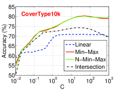
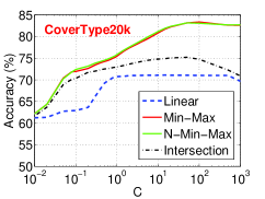
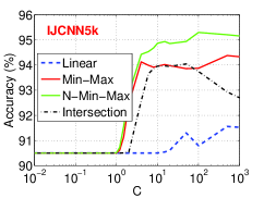
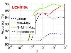
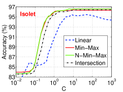
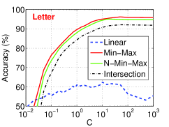
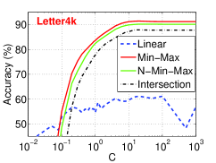
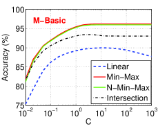
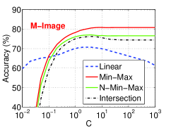
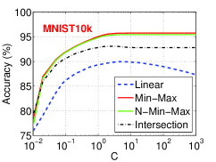
Figure 1: Test classification accuracies for four types of kernels using $l_{2}$-regularized SVM (with a tuning parameter $C$, i..e, the x-axis.). Each panel presents the results for one particular dataset (see more data information in Table 1). The two solid curves represent the min-max kernel (red, if color is available) and the n-min-max kernel (green, if color is available). The dashed curve (blue) and the dot dashed (black) curve represent, respectively, the linear kernel and the intersection kernel. See Figures 2 and 3 for the results on more datasets.

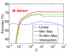
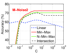
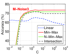
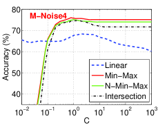
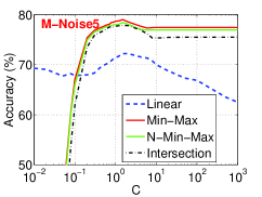
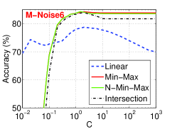
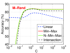
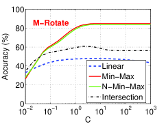
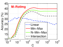
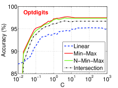
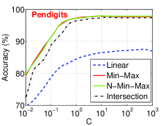
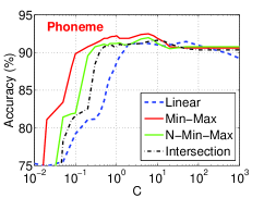
Figure 2: Test classification accuracies for four types of kernels using $l_{2}$-regularized SVM.

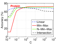
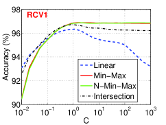
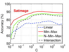
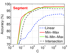
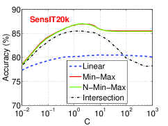
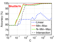
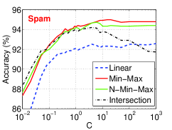
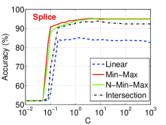
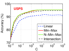
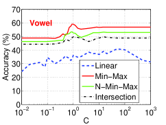
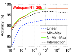
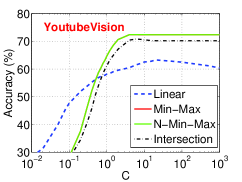
Figure 3: Test classification accuracies for four types of kernels using $l_{2}$-regularized SVM.

Table 1: Classification accuracies (in %) for using 4 different kernels. We use LIBSVM “pre-computed” kernels and $l_{2}$-regularized kernel SVM (which has a tuning parameter $C$). The reported test classification accuracies (i.e., the rightmost 4 columns) are the best accuracies from a wide range of $C$ values; see Figures 1 to 3 for more details. The datasets are all public (and mostly well-known), from various sources including the UCI repository, the LIBSVM web site, the book web site of [12], and the two papers [17, 18] which compared deep nets, boosting and trees, kernel SVMs, etc. (Also see http://hunch.net/?p=1467 for interesting discussions.) Whenever possible, we use the conventional partitions of training and testing sets. We have made efforts to ensure the repeatability of our experiments by using pre-computed kernels and reporting the results for a very wide range of $C$ values. However, this strategy also limits the scale of our experiments because most workstations do not have sufficient memory to store the kernel matrix for datasets of even moderate sizes (for example, a merely $60,000\times 60,000$ kernel matrix has $3.6\times 10^{9}$ entries). Therefore, for the sake of repeatability, for a few datasets we only use a subset of the samples. Please feel free to contact the author if more information is needed in order to reproduce the experiments. Several special notes about the datasets: (i) Whenever possible, we always use the data “as they are” from the sources. Although we agree it is a very important research task to study how to transform the data to favor certain type of similarities, it is not the focus of our paper (and may hurt the repeatability of the experiments if we try to alter the data). (ii) Several datasets downloaded from the LIBSVM site were already scaled to [-1, 1]. To make use of these datasets, we simply transform them by $(z+1)/2$, where $z$ is the original feature value.

Dataset	# train samples	# test samples	linear	min-max	n-min-max	intersection
Covertype10k	10,000	50,000	70.9	80.4	80.2	74.3
Covertype20k	20,000	50,000	71.1	83.3	83.1	75.2
IJCNN5k	5,000	91,701	91.6	94.4	95.3	94.0
IJCNN10k	10,000	91,701	91.6	95.7	96.0	94.5
Isolet	6,238	1,559	95.4	96.4	96.6	96.4
Letter	16,000	4,000	62.4	96.2	95.0	92.1
Letter4k	4,000	16,000	61.2	91.4	90.2	87.9
M-Basic	12,000	50,000	90.0	96.2	96.0	93.4
M-Image	12,000	50,000	70.7	80.8	77.0	76.2
MNIST10k	10,000	60,000	90.0	95.7	95.4	93.1
M-Noise1	10,000	4,000	60.3	71.4	68.5	68.2
M-Noise2	10,000	4,000	62.1	72.4	70.7	70.0
M-Noise3	10,000	4,000	65.2	73.6	71.9	71.6
M-Noise4	10,000	4,000	68.4	76.1	75.2	74.8
M-Noise5	10,000	4,000	72.3	79.0	78.4	77.9
M-Noise6	10,000	4,000	78.7	84.2	84.3	83.9
M-Rand	12,000	50,000	78.9	84.2	84.1	83.7
M-Rotate	12,000	50,000	48.0	84.8	83.9	60.8
M-RotImg	12,000	50,000	31.4	41.0	38.5	37.0
Optdigits	3,823	1,797	95.3	97.7	97.4	96.8
Pendigits	7,494	3,498	87.6	97.9	98.0	97.5
Phoneme	3,340	1,169	91.4	92.5	92.0	91.6
Protein	17,766	6,621	69.1	72.4	70.7	69.6
RCV1	20,242	60,000	96.3	96.9	96.9	96.7
Satimage	4,435	2,000	78.5	90.5	87.8	86.9
Segment	1,155	1,155	92.6	98.1	97.5	97.0
SensIT20k	20,000	19,705	80.5	86.9	87.0	85.5
Shuttle1k	1,000	14,500	90.9	99.7	99.6	99.6
Spam	3,065	1,536	92.6	95.0	94.7	94.2
Splice	1,000	2,175	85.1	95.2	94.9	93.8
USPS	7,291	2,007	91.7	95.3	95.3	94.8
Vowel	528	462	40.9	59.1	53.5	49.8
WebspamN1-20k (1-gram)	20,000	60,000	93.0	97.9	97.8	96.6
YoutubeVision	11,736	10,000	63.3	72.4	72.4	70.8

The purpose of this experimental study on kernel SVMs is not try to show that min-max kernels achieve the best classification accuracies. In fact, compared to trees or deep nets [17, 18], simply using min-max kernels usually does achieve the best accuracies, although the results are close. Since min-max kernels have no tuning parameters, we can expect to boost the performance by using additional parameters or by combining multiple the same (or different) types of kernels. For example, using the idea from CoRE kernels [19], we can multiply min-max kernel with chi-square kernels (which can be hashed by sign cauchy projections [21]).

For large-scale industrial applications, typically it is difficult to directly use (nonlinear) kernels. Fortunately, with CWS (consistent weighted sampling), we can linearize the min-max kernel. In other words, it is possible to achieve the good performance of min-max kernels at the cost of linear kernels. In this paper, we will show how to do CWS better.

3 Hashing Min-Max Kernel

The classification experiments reported in Table 1 and Figures 1 to 3 have demonstrated the effectiveness of min-max kernels in terms of prediction accuracies. However, in order to make min-max kernels practical for large-scale data mining tasks, we need to resort to hashing techniques to (approximately) transform nonlinear kernels into linear kernels.

It is well understood [3] that computing kernels are expensive and the kernel matrix, if fully materialized, does not fit in memory even for relatively small applications. In contrast, highly efficient linear algorithms, e.g., [15, 27, 2, 10], have been widely used in practice for truly large-scale applications such as click predictions in online advertising [25].

3.1 Consistent Weighted Sampling (CWS)

The prior efforts [24, 14] have lead to the method called “consistent weighted sampling (CWS)” for hashing min-max kernels. Here, we adopt the beautiful description of CWS in [14] as shown in Alg. 1.

Input: Data vector $u$ = ($u_{i}\geq 0$, $i=1$ to $D$)

Output: Consistent uniform sample ($i^{*}$, $t^{*}$)

For $i$ from 1 to $D$

$r_{i}\sim Gamma(2,1)$,   $c_{i}\sim Gamma(2,1)$, $\beta_{i}\sim Uniform(0,1)$

$t_{i}\leftarrow\lfloor\frac{\log u_{i}}{r_{i}}+\beta_{i}\rfloor$,  $y_{i}\leftarrow\exp(r_{i}(t_{i}-\beta_{i}))$,  $a_{i}\leftarrow c_{i}/(y_{i}\exp(r_{i}))$

End For

$i^{*}\leftarrow arg\min_{i}\ a_{i}$,         $t^{*}\leftarrow t_{i^{*}}$

Algorithm 1 Consistent Weighted Sampling (CWS)

Given a data vector $u\in\mathbb{R}^{D}$, Alg. 1 provides the procedure for generating one CWS sample $(i^{*},t^{*}$). In order to generate $k$ such samples, we have to repeat the procedure $k$ times using an independent set of random numbers $r_{i}$, $c_{i}$, $\beta_{i}$. For clarity, we denote the samples for data vectors $u$ and $v$ as

$$\left(i^{*}_{u,j},t^{*}_{u,j}\right)\ \text{ and }\ \left(i^{*}_{v,j},t^{*}_{v,j}\right),\ \ j=1,2,...,k$$ (6)

Basically we need to generate 3 matrices: $\{r\}$, $\{c\}$, and $\{\beta\}$, of size $D\times k$. All the data vectors will use the same 3 matrices. This is essentially the same cost as random projections (which however approximate linear kernels).

The basic theoretical result of CWS says the “collision probability” is exactly $K_{MM}$:

$$\mathbf{Pr}\left\{\left(i^{*}_{u,j},t^{*}_{u,j}\right)=\left(i^{*}_{v,j},t^{*}_{v,j}\right)\right\}=K_{MM}(u,v)$$ (7)

Thus, it is clear that, at least conceptually, we can express $K_{MM}(u,v)$ as the expectation of an inner product and hence $K_{MM}$ is positive definite, just like how [22] showed the resemblance is a type of positive definite kernel.

3.2 Drawback of CWS for Data Mining

Although the basic probability result (7) says conceptually we can use CWS for building linear classifiers (approximately in the space of min-max kernels), it is not immediately clear how it can be implemented efficiently.

[14] briefly mentioned that one can “uniformly map” the sample space $(i^{*},t^{*})$ to a space $b$ bits: $\{0,1,2,...,2^{b}-1\}$. This however can not be (easily) achieved. While $i^{*}$ is bounded by $D$, $t^{*}$ is actually unbounded (see Alg. 1). Also note that space of samples is very large. If we represent $i^{*}$ by $b_{i}$ bits and $t^{*}$ (approximately) by $b_{t}$ bits, the space will be $2^{b_{i}+b_{t}}$. Thus, we must find an efficient representation of CWS samples in order to use this nice method effectively for machine learning and data mining applications.

3.3 Our “0-bit” Proposal for CWS

It is now known how to use $b$-bit minwise hashing to approximate the resemblance kernel and use it for large-scale applications [20, 22]. Therefore, in this paper, we focus on representing $t^{*}$. Perhaps surprisingly, our proposal is simple: just ignore $t^{*}$ in the sample $(i^{*},t^{*}$), i.e., the “0-bit” scheme.

If we examine Alg. 1, we can see that $i^{*}$ has already encoded the information about the weights of the data. A rigorous proof however turns out to be a difficult probability problem, which is outside the scope of this paper. Here, we try to empirically demonstrate the following observation:

$$\mathbf{Pr}\left\{i^{*}_{u,j}=i^{*}_{v,j}\right\}\approx\mathbf{Pr}\left\{\left(i^{*}_{u,j},t^{*}_{u,j}\right)=\left(i^{*}_{v,j},t^{*}_{v,j}\right)\right\}$$ (8)

We call our proposal the “0-bit” scheme only to mean that we use 0 bit for coding $t^{*}$. We also call the original proposal as the “full” scheme since it stores all the bits needed for $t^{*}$.

3.4 An Experimental Study on “0-bit” CWS

Table 2: Information of the 13 pairs of English words. For example, “HONG” refers to the vector of occurrences of the word “HONG” in $2^{16}$ documents. $f_{1}$ and $f_{2}$ are the numbers of nonzeros in word 1 and word 2 respectively. For each pair, we include the numerical values for both the resemblance (“$R$”) and the min-max kernel ($MM$).

Word 1	Word 2	$f_{1}$	$f_{2}$	$R$	$MM$
A	THE	39063	42754	0.6444	0.3543
ADDICT	PRICELESS	77	77	0.0065	0.0052
AIR	DOCTOR	3159	860	0.0439	0.0248
CREDIT	CARD	2999	2697	0.2849	0.2091
GAMBIA	KIRIBATI	206	186	0.7118	0.6070
HONG	KONG	940	948	0.9246	0.8985
OF	AND	37339	36289	0.7711	0.6084
PAPER	REVIEW	1944	3197	0.0780	0.0502
PIPELINE	FLUSH	139	118	0.0158	0.0143
SAN	FRANCISCO	3194	1651	0.4758	0.2885
THIS	TODAY	27695	5775	0.1518	0.0658
TIME	JOB	37339	36289	0.1279	0.0794
UNITED	STATES	4079	3981	0.5913	0.5017

Table 2 lists 13 pairs of English words. Each word represents a vector of occurrences of that word in a total of $2^{16}$ documents. This is a typical example of heavy-tailed data in that the weights vary dramatically. In common machine learning applications, the weights often do not vary as much (at least at the point when we are prepared to compute distances/similarites from data). In that sense, we are actually testing our “0-bit” proposal in a more challenging setting.

We have experimented with many more pairs of words than these 13 pairs but the results look essentially the same, i.e., no practical difference between the 0-bit scheme and the full scheme, as can be shown in Figures 4 to 5.

In the experiment, we let $k$ vary from 1 to 1000 and estimate $K_{MM}$ from $k$ measurements $(i^{*}_{,j},t^{*}_{,j})$, $j=1$ to $k$. With the full scheme, we keep all the bits of $t^{*}$. With the 0-bit scheme, we completely discard $t^{*}$. For each $k$, we repeat the simulations $10,000$ times to reliably compute the empirical mean square error (MSE) and the bias for each pair.

The right columns of Figures 4 and 5 plot the empirical MSEs, together with the theoretical variance: $K_{MM}(1-K_{MM})/k$ (i.e., the variance of binomial). Because the curves for the 0-bit scheme and the full scheme overlap the theoretical variances, we can conclude, at least for these data, that our proposed 0-bit scheme is essentially unbiased and the variance matches the theoretical variance of the full scheme.

To avoid many “boring” figures, we let $k$ be as small as 1 (while typical simulations would use a much large number such as 10 to start with). Nevertheless, these MSE curves are still quite boring since all the curves essentially overlap.

To make the presentations somewhat more interesting, we also present the empirical biases in the left columns of the two figures. Now we can see some discrepancies between the two schemes typically on the order of $\ll 10^{-4}$ (in the stabilized zone, i.e., when $k$ is not too small). While such small biases (at the 4th or 5th decimal points) would not make any practical differences, they do serve the purpose to remind us that the 0-bit scheme is indeed an approximation.

To make the plots even more interesting, we add the curves for the “1-bit” scheme (i.e., by recording whether $t^{*}$ is even or odd). For “CREDIT-CARD”, “PIPELINE-FLUSH”, “SAN-FRANCISCO”, and “THIS-TODAY”, we can observe (very small) differences between the 0-bit scheme and the full-scheme. The differences vanish once we use the “1-bit” scheme.

From Table 2, we can see that binarizing the data usually lead to very different similarities (i.e., the last two columns, i.e., $R$ and $MM$, differ significantly). The 0-bit scheme, which only uses $i^{*}$, still very well approximates the original min-max kernel instead of the resemblance kernel. This confirm that, even though our samples (i.e., $i^{*}$) in the same format as samples from minwise hashing (for example, both are integers bounded by $D$), they are statistically very different samples. In other words, our 0-bit scheme is not the same as simply doing the original minwise hashing.

Finally, to entertain readers, we add Figure 6 to report the bias results by keeping all the bits of $t^{*}$ and only a few (0,1,2,4) bits of $i^{*}$. Clearly, only using $t^{*}$ or $t^{*}$ with a few bits of $i^{*}$ will not lead to good estimate of the min-max kernel.

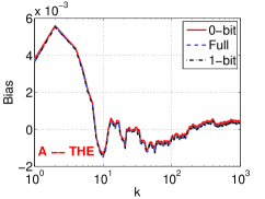
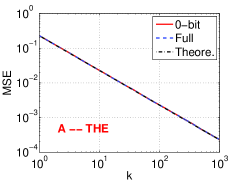
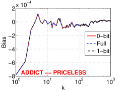
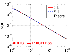
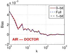
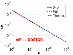
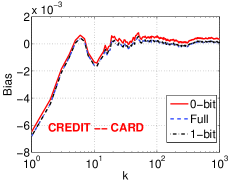
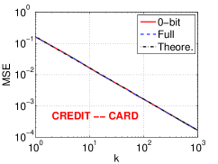
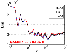
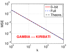
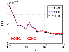
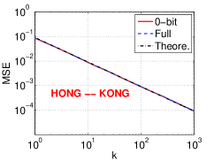
Figure 4: Results for estimating min-max kernels using the “full” scheme by recording all the bits of ($i^{*},t^{*}$) and the “0-bit” scheme by discarding $t^{*}$. For each word pair and $k$, we conducted simulations 10,000 times to compute the mean square errors (MSE) and the biases. The empirical MSE curves (right column) show that both the 0-bit and the full scheme match the theoretical variance. The empirical biases (left column) present a magnified view of errors. For a few pairs (also see Figure 5), the estimations by the 0-bit scheme have noticeable ($\ll 10^{-4}$) biases. By using the “1-bit” scheme (i.e., by recording whether $t^{*}$ is even or odd), these biases vanish.

4 Kernel SVM with Modified CWS

We conduct a set of experiments by using “0-bit” CWS for approximately training min-max kernel SVMs. Basically, for each dataset, we apply CWS hashing for $k$ up to 4096 and, after hashing, we discard $t^{*}$ only keep a matrix of $\{i^{*}\}$, which has the same of number of rows as the number of examples in the dataset and $k$ columns. We then use the popular LIBLINEAR package [10] for training a linear SVM on the data generated by $\{i^{*}\}$, following the scheme proposed by [22].

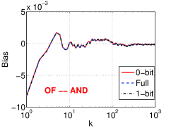
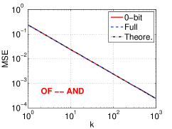
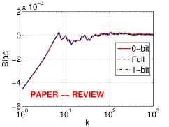
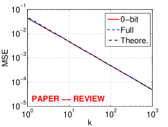
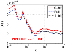
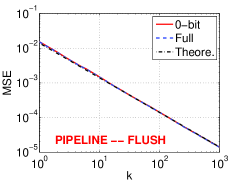
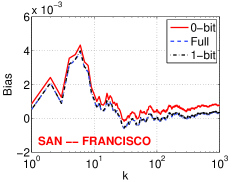
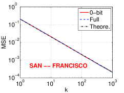
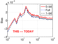
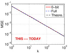
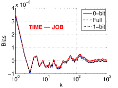
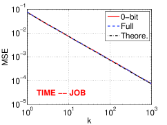
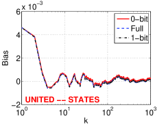
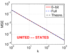
Figure 5: Simulations for estimating min-max kernels. See the caption of Figure 4 for more details.

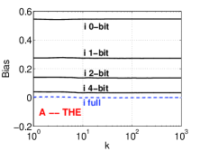
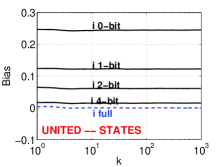
Figure 6: The biases by using full information of $t^{*}$ and only a few (0, 1, 2, or 4) bits of $i^{*}$.

There is one important detail. In practice, since the space $D$ is typically large, we often need to choose to store only a few (say $b_{i}$) bits of $i^{*}$. In other words, after we obtain sample $(i^{*},t^{*})$, we will use $b_{i}$ bits for storing $i^{*}$ and 0 bit for storing $t^{*}$. The effective data matrix will be $2^{b_{i}}\times k$ dimensions with exactly $k$ 1’s in each row. In our experimental study, we always use four choices of $b_{i}\in\{1,2,4,8\}$, corresponding to the four columns (from left to right) in Figures 7 and 8.

Figure 7 presents the linear SVM experiments on a variety of datasets. In each panel, the two dashed curves (red/top and blue/bottom) correspond to the original test accuracies for the min-max kernel and the linear kernel (respectively). In each panel, the solid curves are the results for feeding the 0-bit CWS hashed data to LIBLINEAR, for $k=32,64,128,256,512,1024,2048,4096$ (from bottom to top). For most of the datasets, we can see that the test accuracies approach the results of min-max kernels, when $k$ is large enough, especially if we use 8 bits to store each $i^{*}$.

Figure 8 presents an interesting study for comparing the 0-bit scheme (i.e., $b_{t}=0$ for $t^{*}$) with the 2-bit scheme (i.e., $b_{t}=2$ for $t^{*}$). We can see that once we use $\geq 4$ bits for $i^{*}$, it makes no essential difference whether we use 0-bit or 2-bit scheme for $t^{*}$, i.e., the solid and dashed curves overlap.

5 Discussion and Conclusion

We can view CWS as a tool for “feature engineering” in that it allows practitioners to generate data so that the inner products of the transformed data approximate the min-max kernel values of the original data. We can then utilize extremely efficient and scalable (batch or online) linear methods to equivalently train a nonlinear SVM. In other words, we pay the price of linear learning for nonlinear learning.

For certain applications, linear models based on the original data might be good enough. In that case, if there is a need for dimension reduction, we can use well-known random projection methods. For many datasets (e.g., Table 1), however, linear models are not sufficient and we often have to resort to nonlinear models and computationally intensive procedures. Interestingly, min-max kernels are suitable for many nonnegative datasets, and hence developing efficient ways for approximating min-max kernels becomes useful.

Our contributions consist of three parts. Firstly, we conduct an extensive empirical study of training nonlinear kernel SVMs using min-max kernels, on a wide variety of public datasets. This study answers why we should consider using min-max kernels instead of linear kernels. Secondly, we propose an efficient (and surprisingly simple) implementation of consistent weighted sample, called “0-bit” CWS, and we validate this proposal via an extensive simulation study using real text data. Finally, we show that the 0-bit CWS can be easily integrated into a linear learning system and we demonstrate, on a variety of datasets, that we can achieve the results of nonlinear SVMs by training linear SVMs.

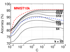
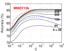
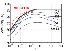
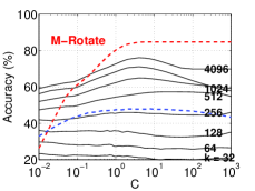
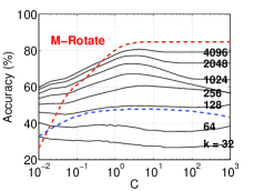
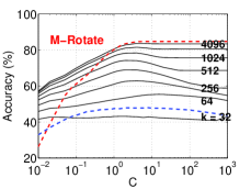
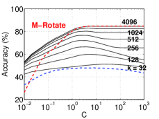
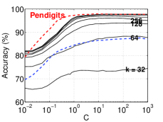
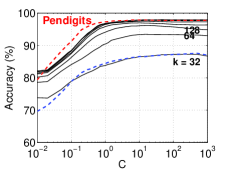
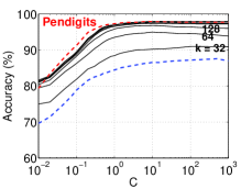
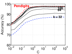
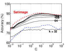
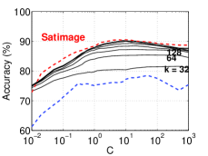
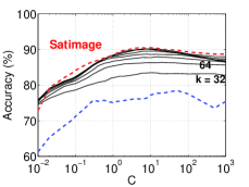
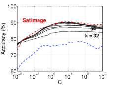
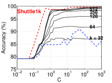
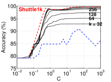
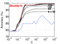
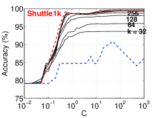
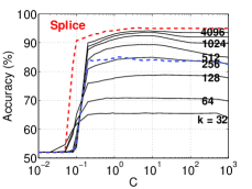
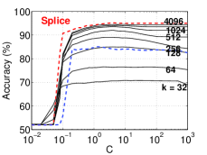
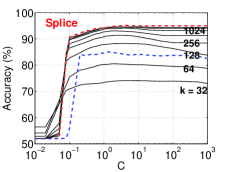
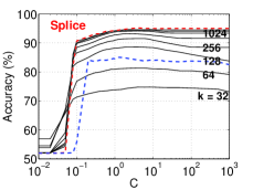
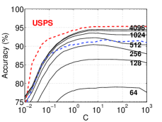
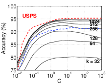
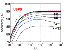
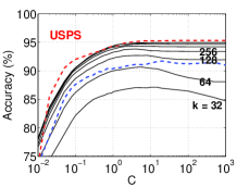
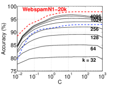
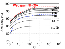
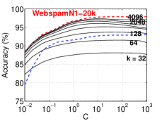
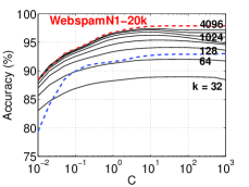
Figure 7: Classification accuracies by using 0-bit CWS hashing and linear SVM. The original CWS algorithm produces samples in the form of $(i^{*},t^{*})$. The 0-bit scheme discards $t^{*}$. From left to right, the four columns represents the results for coding $i^{*}$ using 1 bit, 2 bits, 4 bits, and 8 bits, respectively. In each panel, the two dashed curves represent the original classification results using min-max kernel (top and red) and linear kernel (bottom and blue). The solid curves are the results of linear SVM and 0-bit CWS with $k=32$, 64, 128, 256, 512, 1024, 2048, 4096 (from bottom to top).

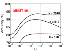
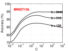
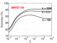
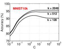
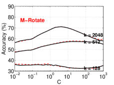
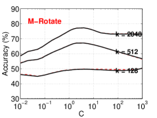
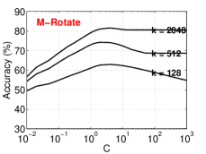
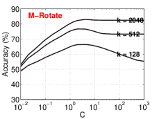
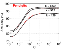
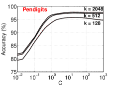
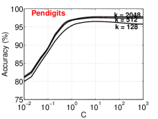
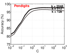
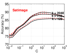
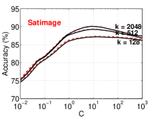
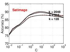
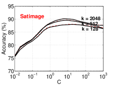
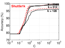
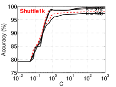
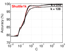
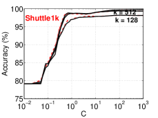
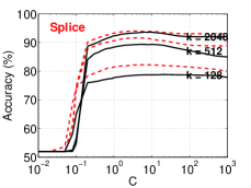
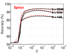
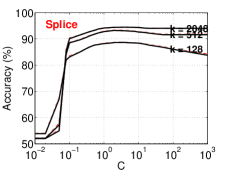
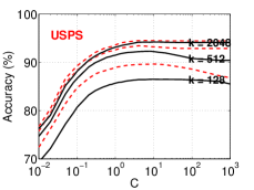
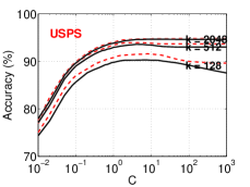
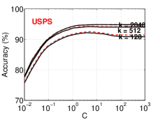
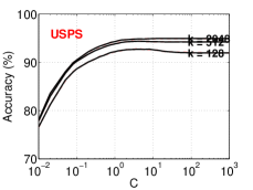
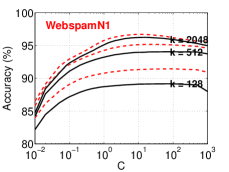
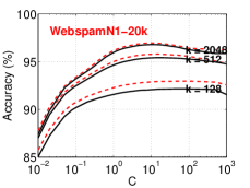
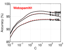
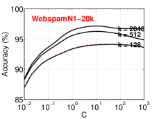
Figure 8: Classification accuracies by using linear SVM with 0-bit CWS (solid and black curves) and 2-bit CWS (dashed and red curves). The original CWS algorithm produces samples in the form of $(i^{*},t^{*})$. The 0-bit scheme discards $t^{*}$ while the 2-bit scheme keeps 2 bits for each $t^{*}$. From left to right, the four columns represent the results for coding $i^{*}$ using 1 bit, 2 bits, 4 bits, and 8 bits, respectively. In each panel, the 3 solid curves (0-bit scheme for $k=$128, 512, 2048) and the 3 dashed curves (2-bit scheme) essentially overlap especially when we use $\geq 4$ bits for coding $i^{*}$.

References

- [1] R. J. Bayardo, Y. Ma, and R. Srikant. Scaling up all pairs similarity search. In WWW, pages 131–140, 2007.
- [2] L. Bottou. http://leon.bottou.org/projects/sgd.
- [3] L. Bottou, O. Chapelle, D. DeCoste, and J. Weston, editors. Large-Scale Kernel Machines. The MIT Press, Cambridge, MA, 2007.
- [4] A. Z. Broder. On the resemblance and containment of documents. In the Compression and Complexity of Sequences, pages 21–29, Positano, Italy, 1997.
- [5] A. Z. Broder, S. C. Glassman, M. S. Manasse, and G. Zweig. Syntactic clustering of the web. In WWW, pages 1157 – 1166, Santa Clara, CA, 1997.
- [6] L. Cherkasova, K. Eshghi, C. B. M. III, J. Tucek, and A. C. Veitch. Applying syntactic similarity algorithms for enterprise information management. In KDD, pages 1087–1096, Paris, France, 2009.
- [7] F. Chierichetti, R. Kumar, S. Lattanzi, M. Mitzenmacher, A. Panconesi, and P. Raghavan. On compressing social networks. In KDD, pages 219–228, Paris, France, 2009.
- [8] G. Cormode and S. Muthukrishnan. Space efficient mining of multigraph streams. In Proceedings of the twenty-fourth ACM SIGMOD-SIGACT-SIGART symposium on Principles of database systems, pages 271–282. ACM, 2005.
- [9] A. S. Das, M. Datar, A. Garg, and S. Rajaram. Google news personalization: scalable online collaborative filtering. In Proceedings of the 16th international conference on World Wide Web, pages 271–280. ACM, 2007.
- [10] R.-E. Fan, K.-W. Chang, C.-J. Hsieh, X.-R. Wang, and C.-J. Lin. Liblinear: A library for large linear classification. Journal of Machine Learning Research, 9:1871–1874, 2008.
- [11] G. Forman, K. Eshghi, and J. Suermondt. Efficient detection of large-scale redundancy in enterprise file systems. SIGOPS Oper. Syst. Rev., 43(1):84–91, 2009.
- [12] T. J. Hastie, R. Tibshirani, and J. H. Friedman. The Elements of Statistical Learning:Data Mining, Inference, and Prediction. Springer, New York, NY, 2001.
- [13] M. R. Henzinger. Finding near-duplicate web pages: a large-scale evaluation of algorithms. In SIGIR, pages 284–291, 2006.
- [14] S. Ioffe. Improved consistent sampling, weighted minhash and L1 sketching. In ICDM, pages 246–255, Sydney, AU, 2010.
- [15] T. Joachims. Training linear svms in linear time. In KDD, pages 217–226, Pittsburgh, PA, 2006.
- [16] N. Koudas, S. Sarawagi, and D. Srivastava. Record linkage: similarity measures and algorithms. In Proceedings of the 2006 ACM SIGMOD international conference on Management of data, pages 802–803. ACM, 2006.
- [17] H. Larochelle, D. Erhan, A. C. Courville, J. Bergstra, and Y. Bengio. An empirical evaluation of deep architectures on problems with many factors of variation. In ICML, pages 473–480, Corvalis, Oregon, 2007.
- [18] P. Li. Robust logitboost and adaptive base class (abc) logitboost. In UAI, 2010.
- [19] P. Li. CoRE kernels. In UAI, Quebec City, CA, 2014.
- [20] P. Li and A. C. König. b-bit minwise hashing. In Proceedings of the 19th International Conference on World Wide Web, pages 671–680, Raleigh, NC, 2010.
- [21] P. Li, G. Samorodnitsky, and J. Hopcroft. Sign cauchy projections and chi-square kernel. In NIPS, Lake Tahoe, NV, 2013.
- [22] P. Li, A. Shrivastava, J. Moore, and A. C. König. Hashing algorithms for large-scale learning. In NIPS, Granada, Spain, 2011.
- [23] S. Maji, A. Berg, and J. Malik. Classification using intersection kernel support vector machines is efficient. In CVPR, pages 1–8, 2008.
- [24] M. Manasse, F. McSherry, and K. Talwar. Consistent weighted sampling. Technical Report MSR-TR-2010-73, Microsoft Research, 2010.
- [25] H. B. McMahan, G. Holt, D. Sculley, M. Young, D. Ebner, J. Grady, L. Nie, T. Phillips, E. Davydov, D. Golovin, S. Chikkerur, D. Liu, M. Wattenberg, A. M. Hrafnkelsson, T. Boulos, and J. Kubica. Ad click prediction: A view from the trenches. In KDD, pages 1222–1230, 2013.
- [26] S. Pandey, A. Broder, F. Chierichetti, V. Josifovski, R. Kumar, and S. Vassilvitskii. Nearest-neighbor caching for content-match applications. In WWW, pages 441–450, Madrid, Spain, 2009.
- [27] S. Shalev-Shwartz, Y. Singer, and N. Srebro. Pegasos: Primal estimated sub-gradient solver for svm. In ICML, pages 807–814, Corvalis, Oregon, 2007.
- [28] T. Urvoy, E. Chauveau, P. Filoche, and T. Lavergne. Tracking web spam with html style similarities. ACM Trans. Web, 2(1):1–28, 2008.