Optimisation of Quantum Hamiltonian Evolution:
From Two Projection Operators to Local Hamiltonians

Abstract

Given a quantum Hamiltonian and its evolution time, the corresponding unitary evolution operator can be constructed in many different ways, corresponding to different trajectories between the desired end-points and different series expansions. A choice among these possibilities can then be made to obtain the best computational complexity and control over errors. It is shown how a construction based on Grover’s algorithm scales linearly in time and logarithmically in the error bound, and is exponentially superior in error complexity to the scheme based on the straightforward application of the Lie-Trotter formula. The strategy is then extended first to simulation of any Hamiltonian that is a linear combination of two projection operators, and then to any local efficiently computable Hamiltonian. The key feature is to construct an evolution in terms of the largest possible steps instead of taking small time steps. Reflection operations and Chebyshev expansions are used to efficiently control the total error on the overall evolution, without worrying about discretisation errors for individual steps. We also use a digital implementation of quantum states that makes linear algebra operations rather simple to perform.

Keywords: Baker-Campbell-Hausdorff expansion; Digital representation; Grover’s algorithm; Hamiltonian evolution; Lie-Trotter formula; Projection and reflection operators; Chebyshev polynomials.

1 Introduction

Richard Feynman advocated development of quantum computers as efficient simulators of physical quantum systems [1]. Real physical systems are often replaced by simplified models in order to understand their dynamics. Even then, exact solutions are frequently not available, and it has become commonplace to study the models using elaborate computer simulations. Classical computer simulations of quantum models are not efficient—well-known examples range from the Hubbard model to lattice QCD—and Feynman argued that quantum simulations would do far better.

As a concrete realisation of Feynman’s argument, it is convenient to look at Hamiltonian evolution of a many-body quantum system. Quantum simulations can sum multiple evolutionary paths contributing to a quantum process in superposition at one go, while classical simulations need to evaluate these paths one by one. Formalisation of this advantage, in terms of computational complexity, has gradually improved over the years. Real physical systems are governed by local Hamiltonians, i.e. where each component interacts only with a limited number of its neighbours independent of the overall size of the system. Lloyd constructed a quantum evolution algorithm for such systems [2], based on the discrete time Lie-Trotter decomposition of the unitary evolution operator, and showed that it is efficient in the required time and space resources. Aharonov and Ta-Shma rephrased the problem as quantum state generation, treating the terms in the Hamiltonian as black box oracles, and extended the result to sparse Hamiltonians in graph theoretical language [3]. The time complexity of the algorithm was then improved [4, 5, 6], using Suzuki’s higher order generalisations of the Lie-Trotter formula [7] and clever decompositions of the Hamiltonian. Recently the error complexity of the evolution has been reduced from power-law to logarithmic in the inverse error, using the strategy of discrete time simulation of multi-query problems [8]. This is a significant jump in computational complexity improvement that needs elaboration and understanding. In this article, we explicitly construct efficient evolution algorithms first for Hamiltonians that are linear combinations of two projection operators, to expose the physical reasons behind the improvement, and then extend the strategy to any local efficiently computable Hamiltonian. Our constructive methods differ from the reductionist approach of Ref. [8], we improve upon earlier results, and clearly demonstrate how the algorithms work in practice.

Computational complexity of a problem is a measure of the resources needed to solve it. Conventionally, the computational complexity of a decision problem is specified in terms of the size of its input, noting that the size of its output is only one bit. This framework is extended to problems with different output requirements (e.g. find the optimal route for the travelling salesman problem or evaluate $\pi$ to a certain precision), by setting up successive verifiable bounds on the outputs. For example, the problem of evaluating $\pi$ can be implemented as first confirming that $\pi\in[3,4]$, and then narrowing down the interval by bisection, adding one bit of precision for every decision made. In such a scenario, the number of decision problems solved equals the number of output bits, and the complexity of the original problem is the sum of the complexities for the individual decision problems. It is therefore appropriate to specify the complexity of the original problem in terms of the size of its input as well as its output, especially for function evaluation problems. Generalizing the conventional classification, the computational algorithm can then be labeled efficient if the required resources are polynomial in terms of the size of both its input and its output. We label such algorithms as belonging to the class P:P, explicitly expressing their computational complexity with respect to their input as well as output sizes. Simultaneous consideration of both input and output dependence of complexity is natural for reversible computation. It is also necessary when extending finite precision analog computation to arbitrary precision digital computation. Note that our definition of P:P efficiency differs from the concept of “simulatable Hamiltonians” in Ref. [3].

The traditional computational complexity analysis (e.g. P vs. NP classification) does not discuss much how the complexity depends on the output precision, and the task is relegated to design of efficient methods for arbitrary precision numerical analysis [9]. We stress that both input and output size dependence of the computational complexity are equally important for practical function evaluation problems. Popular importance sampling methods are not efficient according to our criterion, because the number of iterations needed in the computational effort has a negative power-law dependence on the precision $\epsilon$ (i.e. $N_{\rm iter}\propto\epsilon^{-2}$ as per the central limit theorem). On the other hand, finding zeroes of a function by bisection is efficient (i.e. $N_{\rm iter}\propto\log\epsilon$), and finding them by Newton’s method is super-efficient (i.e. $N_{\rm iter}\propto\log\log\epsilon$).

We describe the Hamiltonian simulation problem in Section 2, along with the important ingredients required for its optimisation. In Section 3, we formulate the database search problem as Hamiltonian evolution. While the evolution results are well-known (see for instance Refs. [10, 11]), we focus on the error complexity which has not been optimised in the literature. Our analysis explicitly shows how Grover’s large time-step algorithm is exponentially superior to small time-step algorithms approximating continuous time evolution. It also demonstrates that the large time-step algorithm effectively simulates a very different Hamiltonian than the small time-step algorithm, but yields the same total evolution operator [12]. As an important ingredient, we introduce digital representation for quantum states that makes performing linear algebra operations with them straightforward. In Section 4, we construct a series expansion evolution algorithm for Hamiltonians that are linear combinations of two projection operators. We carry out a partial summation of the series, and demonstrate how evaluation of a truncated series of large-step reflection operators improves the error complexity exponentially compared to the small-step Lie-Trotter formula. Our analytic results are supported by numerical tests. Finally in Section 5, we combine the methods of Chebyshev series expansion and digital representation, to construct an efficient simulation algorithm for any local efficiently computable Hamiltonian. We conclude with an outlook for our methods, and some general results for projection operators are collected in an Appendix.

2 Quantum Hamiltonian Simulation

The Hamiltonian simulation problem is to evolve an initial quantum state $|\psi(0)\rangle$ to a final quantum state $|\psi(T)\rangle$, in presence of interactions specified by a Hamiltonian $H(t)$:

$$|\psi(T)\rangle=U(T)|\psi(0)\rangle~{},~{}~{}U(T)={\cal P}\Big{[}\exp\big{(}-i\int_{0}^{T}H(t)dt\big{)}\Big{]}~{}.$$ (1)

The initial state can often be prepared easily, while the final state is generally unknown. The path ordering of the unitary evolution operator $U(T)$, denoted by the symbol ${\cal P}$ in Eq.(1), is necessary when various terms in the Hamiltonian do not commute. The properties of the final state are subsequently obtained from expectation values of various observables:

$$\langle O_{a}\rangle=\langle\psi(T)|O_{a}|\psi(T)\rangle~{}.$$ (2)

In typical problems of quantum dynamics, both these parts—the final state and the expectation values—are determined probabilistically upto a specified tolerance level. They also require different techniques, and so it is convenient to deal with them separately. In this article, we focus only on the former part; the latter part has been addressed in Refs. [13, 14], and still needs exponential improvement in the dependence of computational complexity on the output precision to belong to the class P:P. For simplicity, we also restrict ourselves to problems where both the Hamiltonian $H$ and the observables $O_{a}$ are bounded.

It is also possible to define the Hamiltonian simulation problem as the determination of the evolution operator $U(T)$, and omit any mention of the initial and the final states. The accuracy of the simulation is then specified by the norm of the difference between simulated and exact evolution operators, say $||\widetilde{U}(T)-U(T)||<\epsilon$. In actual implementation, the simulated $\widetilde{U}(T)$ may not be exactly unitary, due to round-off and truncation errors, but the preceding measure for the accuracy of the simulation still suffices as long as $\epsilon$ is small enough.

We concern ourselves here only with Hamiltonians acting in finite $N$-dimensional Hilbert spaces. A general Hamiltonian would then be a dense $N\times N$ matrix, and there is no efficient way to simulate it. So we restrict the Hamiltonian according to the following features commonly present in physical problems:
(1) The Hilbert space is a tensor product of many small components, e.g. $N=2^{n}$ for a system of $n$ qubits.
(2) The components have only local interactions irrespective of the size of the system, e.g. only nearest neighbour couplings. That makes the Hamiltonian sparse, with $O(N)$ non-zero elements.
(3) The Hamiltonian is specified in terms of a finite number of efficiently computable functions, while the arguments of the functions can depend on the components, e.g. the interactions are translationally invariant.
These features follow the notion of Kolmogorov complexity, where the computational resources needed to describe an object are quantified in terms of the compactness of the description. With a compact description of the Hamiltonian, the resources needed to just write it down do not influence the simulation complexity.

Such sparse Hamiltonians can be mapped to graphs with bounded degree $d$, with the vertices representing the physical components of the system and the edges denoting the interactions between neighbouring components. Their simulations can be easily parallelised—on classical computers, Hamiltonians with these features allow SIMD simulations with domain decomposition.

We note that long range physical interactions do exist, but simulation of generic dense Hamiltonians is not efficient [15]. Only with some extra properties, dense Hamiltonians can lead to non-local evolution operators having compact descriptions. A useful example is FFT, which describes a dense but factorisable unitary transformation that can be efficiently implemented, but we do not consider such possibilities here.

With all these specifications, efficient Hamiltonian simulation algorithms in the class P:P use computational resources that are polynomial in $\log(N)$, $d$ and $\log(\epsilon)$.

2.1 Hamiltonian Decomposition

Efficient simulation strategy for Hamiltonian evolution has two major ingredients. In general, exponential of a sparse Hamiltonian is not sparse, which makes exact evaluation of $\exp(-iHt)$ difficult. So the first ingredient is to decompose the sparse Hamiltonian as a sum of non-commuting but block-diagonal Hermitian operators, i.e. $H=\sum_{i=1}^{l}H_{i}$. The motivation for such a decomposition is twofold:

(a) Functions of individual $H_{i}$, defined as power series, can be easily and exactly calculated for any time evolution $\tau$, and they retain the same block-diagonal structure.

(b) The blocks are decoupled and so can be evolved simultaneously, in parallel (classically) or in superposition (quantum mechanically).

Furthermore, the blocks can be reduced in size all the way to a mixture of $1\times 1$ and $2\times 2$ blocks. The $1\times 1$ blocks just produce phases upon exponentiation, while the $2\times 2$ blocks can be expressed as linear combinations of identity and projection or reflection operators (i.e. $(1+\hat{n}\cdot\vec{\sigma})/2$ or $\hat{n}\cdot\vec{\sigma}$ respectively, where $\hat{n}$ is a unit vector and $\sigma_{i}$ are the three Pauli matrices). There is no loss of generality in such a choice; it is just a convenient choice of basis that simplifies the subsequent algorithm. Projection or reflection operators with only two distinct eigenvalues can be interpreted as binary query oracles. Their large spectral gaps also help in rapid convergence of series expansions involving them.

In general, $H_{i}$ can be systematically identified by an edge-colouring algorithm for graphs [3], with distinct colours (labeled by the index $i$) for overlapping edges. As per Vizing’s theorem, any simple graph of degree $d$ can be efficiently coloured with $d+1$ colours. Physical models are often defined on bipartite graphs, for which the colouring algorithms are simpler than those for general graphs and need $d$ colours. Identification of $H_{i}$ also provides a compressed labeling scheme that can be used to address individual blocks.

Actual calculations do not need explicit construction of $U(T)$, rather only the effect of $U(T)$ on the quantum state $|\psi(0)\rangle$ has to be evaluated. That is accomplished by breaking down the calculation into steps, each of which consists of the product of a sparse matrix with a vector, e.g. $\exp(-iH_{i}\tau)|\psi\rangle$. The simulation complexity is then conveniently counted in units of such sparse matrix-vector products.

As a simple illustration, the discretised Laplacian for a one-dimensional lattice has the block-diagonal decomposition given by:

$$\left(\matrix{\cdots&\cdots&\cdots&\cdots&\cdots&\cdots&\cdots\cr\cdots&\hfill-1&\hfill 2&\hfill-1&\hfill 0&\hfill 0&\cdots\cr\cdots&\hfill 0&\hfill-1&\hfill 2&\hfill-1&\hfill 0&\cdots\cr\cdots&\hfill 0&\hfill 0&\hfill-1&\hfill 2&\hfill-1&\cdots\cr\cdots&\cdots&\cdots&\cdots&\cdots&\cdots&\cdots\cr}\right)$$ (3)

$$= \left(\matrix{\cdots&\cdots&\cdots&\cdots&\cdots&\cdots&\cdots\cr\cdots&\hfill-1&\hfill 1&\hfill 0&\hfill 0&\hfill 0&\cdots\cr\cdots&\hfill 0&\hfill 0&\hfill 1&\hfill-1&\hfill 0&\cdots\cr\cdots&\hfill 0&\hfill 0&\hfill-1&\hfill 1&\hfill 0&\cdots\cr\cdots&\cdots&\cdots&\cdots&\cdots&\cdots&\cdots\cr}\right)+\left(\matrix{\cdots&\cdots&\cdots&\cdots&\cdots&\cdots&\cdots\cr\cdots&\hfill 0&\hfill 1&\hfill-1&\hfill 0&\hfill 0&\cdots\cr\cdots&\hfill 0&\hfill-1&\hfill 1&\hfill 0&\hfill 0&\cdots\cr\cdots&\hfill 0&\hfill 0&\hfill 0&\hfill 1&\hfill-1&\cdots\cr\cdots&\cdots&\cdots&\cdots&\cdots&\cdots&\cdots\cr}\right).$$

This decomposition, $H=H_{o}+H_{e}$, has the projection operator structure following from $H_{o}^{2}=2H_{o}$ and $H_{e}^{2}=2H_{e}$. Graphically, the break-up can be represented as:

where $H_{o}$ and $H_{e}$ are identified by the last bit of the position label. Eigenvalues of $H$ are $4\sin^{2}(k/2)$ in terms of the lattice momentum $k$, while those of $H_{o}$ and $H_{e}$ are just $0$ and $2$.

2.2 Evolution Optimisation

Given that individual $H_{i}$ can be exponentiated exactly and efficiently, their sum $H$ can be approximately exponentiated using the discrete Lie-Trotter formula:

$$\exp\big{(}-iHT\big{)} = \exp\Big{(}-i\sum_{i}H_{i}T\Big{)}$$

$$\approx \Big{(}\prod_{i}\exp(-iH_{i}\Delta t)\Big{)}^{m}~{},~{}~{}m=T/\Delta t~{}.$$

This replacement maintains unitarity of the evolution exactly, but may not preserve other properties such as the energy. The accuracy of the approximation is commonly improved by making $\Delta t$ sufficiently small, sometimes accompanied by higher order discretisations. This approach has been used for classical parallel computer simulations of quantum evolution problems [16, 17].

In contrast, the second ingredient of efficient Hamiltonian simulation is to use as large $\Delta t$ as possible. When the exponent is proportional to a projection operator, the largest $\Delta t$ is the one that makes the exponential a reflection operator. In general, use of any fixed constant $\Delta t$ changes the leading scaling behaviour of the error complexity from a power-law dependence on $\epsilon$ to a logarithmic one. The extreme strategy of choosing the largest possible $\Delta t$ not only keeps the evolution accurate by reducing the round-off and the truncation errors, but also optimises the scaling proportionality constant. It is not at all obvious how such a result may arise, and so we demonstrate it first in Section 3 using the database search problem as an explicit example, and then in Section 4 for Hamiltonians that are a linear combination of two more general projection operators.

Our efficient Hamiltonian simulation algorithms, explicitly constructed using the two ingredients just described, have computational complexity

$$O\left(t\frac{\log(t/\epsilon)}{\log(\log(t/\epsilon))}{\cal C}\right)~{}.$$ (5)

Here ${\cal C}$ is the computational cost of a single time step, which only weakly depends on $t$ and $\epsilon$. It is ${\cal C}$ that characterises how computational complexity of classical implementation is improved in the quantum case, through conversion of independent parallel execution threads into quantum superposition. We point out that to keep the discretisation error under control, digital calculations need $b$-bit precision, with $b=\Omega(\log((t/\epsilon)\log(t/\epsilon)))$. For $l$-sparse Hamiltonians whose elements can be evaluated efficiently, the computational cost ${\cal C}$ is $O(lNb^{3})$ classically and $O(lnb^{3})$ quantum mechanically.

3 Quantum Database Search as Hamiltonian Evolution

The quantum database search algorithm works in an $N$-dimensional Hilbert space, whose basis vectors are identified with the individual items. It takes an initial state whose amplitudes are uniformly distributed over all the items, to the target state where all but one amplitudes vanish. Let $\{|i\rangle\}$ be the set of basis vectors, $|s\rangle$ be the initial uniform superposition state, and $|t\rangle$ be the target state corresponding to the desired item. Then

$$|\psi(0)\rangle=|s\rangle~{},~{}~{}|\psi(T)\rangle=|t\rangle~{},$$

$$|\langle i|s\rangle|=1/\sqrt{N}~{},~{}~{}\langle i|t\rangle=\delta_{it}~{}.$$ (6)

The simplest evolution schemes taking $|s\rangle$ to $|t\rangle$ are governed by time-independent Hamiltonians that depend only on $|s\rangle$ and $|t\rangle$. The unitary evolution is then a rotation in the two-dimensional subspace, formed by $|s\rangle$ and $|t\rangle$, of the whole Hilbert space. In this subspace, let

$$|t\rangle=\pmatrix{1}\\ 0~{},~{}~{}|t_{\perp}\rangle=\pmatrix{0}\\ 1~{},~{}~{}|s\rangle=\pmatrix{1}/\sqrt{N}\\ \sqrt{(N-1)/N}~{}.$$ (7)

On the Bloch sphere representing the density matrix, the states $|s\rangle\langle s|$ and $|t\rangle\langle t|$ are respectively given by the unit vectors $\hat{n}_{s}=\big{(}\frac{2\sqrt{N-1}}{N},0,\frac{2}{N}-1\big{)}$ and $\hat{n}_{t}=(0,0,1)$. The angle between them is $\cos^{-1}(\frac{2}{N}-1)$, which is twice the angle $\cos^{-1}(1/\sqrt{N})$ between $|s\rangle$ and $|t\rangle$ in the Hilbert space.

For a time-independent Hamiltonian, the time evolution of the state is a rotation at a fixed rate around a direction specified by the Hamiltonian:

$$U(t)=\exp(-iHt)=\exp(-i\hat{n}_{H}\cdot\vec{\sigma}~{}\omega t)~{}.$$ (8)

For the database search problem, $U(T)|s\rangle=|t\rangle$, upto a phase arising from a global additive constant in the Hamiltonian. There are many possible evolution routes from the initial to the target state, and we consider two particular cases in turn.

3.1 Farhi-Gutmann’s and Grover’s Algorithms

Grover based his algorithm on a physical intuition [18], where the potential energy term in the Hamiltonian attracts the wavefunction towards the target state and the kinetic energy term in the Hamiltonian diffuses the wavefunction over the whole Hilbert space. Both the potential energy $|t\rangle\langle t|$ and the kinetic energy $|s\rangle\langle s|$ terms are projection operators. The corresponding time-independent Hamiltonian is

$$H_{C}=|s\rangle\langle s|+|t\rangle\langle t| = \pmatrix{1+\frac{1}{N}&\frac{\sqrt{N-1}}{N}\cr\frac{\sqrt{N-1}}{N}&1-\frac{1}{N}}$$

$$= I+\frac{\sqrt{N-1}}{N}\sigma_{1}+\frac{1}{N}\sigma_{3}~{}.$$

That gives rise to the evolution operator (omitting the global phase)

$$U_{C}(t) = \exp\big{(}-i\hat{n}\cdot\vec{\sigma}~{}t/\sqrt{N}\big{)}$$ (10)

$$= \cos(t/\sqrt{N})-i\hat{n}\cdot\vec{\sigma}\sin(t/\sqrt{N})~{},$$

which is a rotation on the Bloch sphere by angle $2t/\sqrt{N}$ around the direction $\hat{n}=\big{(}\sqrt{(N-1)/N},0,1/\sqrt{N}\big{)}^{T}$.

The (unnormalised) eigenvectors of $H_{C}$ are $|s\rangle\pm|t\rangle$, which are the orthogonal states left invariant by the evolution operator $U_{C}(t)$. On the Bloch sphere, their density matrices point in the directions $\pm\hat{n}$, which bisect the initial and the target states, $|s\rangle\langle s|$ and $|t\rangle\langle t|$. Thus a rotation by angle $\pi$ around the direction $\hat{n}$ takes $|s\rangle\langle s|$ to $|t\rangle\langle t|$ on the Bloch sphere. In the Hilbert space, the rotation angle taking $|s\rangle$ to $|t\rangle$ is then $\pi/2$, and so the time required for the Hamiltonian search is $T=(\pi/2)\sqrt{N}$ [19].

Grover made an enlightened jump from this scenario, motivated by the Lie-Trotter formula. He exponentiated the projection operators in $H_{C}$ to reflection operators; $R=\exp(\pm i\pi P)=1-2P$ for any projection operator $P$. The optimal algorithm that Grover discovered iterates the discrete evolution operator [20],

$$U_{G} = -(1-2|s\rangle\langle s|)(1-2|t\rangle\langle t|)$$ (11)

$$= \pmatrix{1-\frac{2}{N}&2\frac{\sqrt{N-1}}{N}\cr-2\frac{\sqrt{N-1}}{N}&1-\frac{2}{N}}=(1-\frac{2}{N})I+2i\frac{\sqrt{N-1}}{N}\sigma_{2}~{}.$$

With $U_{G}=\exp(-iH_{G}\tau)$, it corresponds to the evolution Hamiltonian

$$H_{G} = \frac{i}{\sqrt{N}}\big{(}|t\rangle\langle s|-|s\rangle\langle t|\big{)}$$ (12)

$$= \pmatrix{0&i\frac{\sqrt{N-1}}{N}\cr-i\frac{\sqrt{N-1}}{N}&0}=-\frac{\sqrt{N-1}}{N}\sigma_{2}~{},$$

and the evolution step

$$\tau=\frac{N}{\sqrt{N-1}}\sin^{-1}\Big{(}2\frac{\sqrt{N-1}}{N}\Big{)}=\frac{2N}{\sqrt{N-1}}\sin^{-1}\Big{(}\frac{1}{\sqrt{N}}\Big{)}~{}.$$ (13)

It is an important non-trivial fact that $H_{G}$ is the commutator of the two projection operators in $H_{C}$:

$$H_{G}=i\big{[}|t\rangle\langle t|,|s\rangle\langle s|\big{]}~{}.$$ (14)

This commutator is the leading correction to the Lie-Trotter formula in the Baker-Campbell-Hausdorff (BCH) expansion [21], making Grover’s algorithm an ingenious summation of the BCH expansion for the evolution operator.

On the Bloch sphere, each $U_{G}$ step is a rotation by angle $2\tau\sqrt{N-1}/N=4\sin^{-1}(1/\sqrt{N})$ around the direction $\hat{n}_{G}=(0,1,0)^{T}$, taking the geodesic route from the initial to the final state. That makes the number of steps required for this discrete Hamiltonian search,

$$Q_{T} = \frac{1}{4}\cos^{-1}\Big{(}\frac{2}{N}-1\Big{)}\Big{/}\sin^{-1}\Big{(}\frac{1}{\sqrt{N}}\Big{)}$$ (15)

$$= \frac{\cos^{-1}(1/\sqrt{N})}{2\sin^{-1}(1/\sqrt{N})}\approx\frac{\pi}{4}\sqrt{N}~{}.$$

Figure 1: Evolution trajectories on the Bloch sphere for the quantum database search problem, going from $|s\rangle$ to $|t\rangle$. The Hamiltonians $H_{C}$ and $H_{G}$ generate rotations around the directions $\hat{n}$ and $\hat{n}_{G}$ respectively.

Note that $\hat{n}$ and $\hat{n}_{G}$ are orthogonal, so the evolution trajectories produced by rotations around them are completely different from each other, as illustrated in Fig.1. It is only after a specific evolution time, corresponding to the solution of the database search problem, that the two trajectories meet each other. The evolution operators in the two cases are:

$$U_{C}(T)=\exp\Big{(}-i\hat{n}\cdot\sigma\frac{\pi}{2}\Big{)}=-i\pmatrix{\frac{1}{\sqrt{N}}&\sqrt{\frac{N-1}{N}}\cr\sqrt{\frac{N-1}{N}}&-\frac{1}{\sqrt{N}}\cr}~{},$$ (16)

$$(U_{G})^{Q_{T}}=\exp\Big{(}i\cos^{-1}\Big{(}\frac{1}{\sqrt{N}}\Big{)}\sigma_{2}\Big{)}=\pmatrix{\frac{1}{\sqrt{N}}&\sqrt{\frac{N-1}{N}}\cr-\sqrt{\frac{N-1}{N}}&\frac{1}{\sqrt{N}}\cr}~{}.$$ (17)

The rates of different Hamiltonian evolutions can be compared only after finding a common convention to fix the magnitude and the ease of simulation of the Hamiltonians:

(1) Magnitude: A global additive shift of the Hamiltonian has no practical consequence. So possible comparison criteria can be the norm of the traceless part of the Hamiltonian or the spectral gap over the ground state. $||H_{C}||=1/\sqrt{N}$ and $||H_{G}||=\frac{\sqrt{N-1}}{N}$ are comparable, with the same limit as $N\rightarrow\infty$.

(2) Ease of simulation: The binary query oracle can be used to produce various functions of $|t\rangle\langle t|$.

(a) $H_{C}$ can be easily simulated by alternating small evolution steps governed by $|s\rangle\langle s|$ and $|t\rangle\langle t|$, according to the Lie-Trotter formula [22]. Each evolution step governed by $|t\rangle\langle t|$ needs two binary query oracles, as shown in Fig.2.

(b) $U_{G}$ is easily obtained using one binary query oracle per evolution step.

Figure 2: Quantum logic circuit for the fractional query oracle operator $O_{\phi}=\exp(i\phi|t\rangle\langle t|)$. The oracle flips the ancilla bit iff its input is the target state, and the standard binary query oracle operator corresponds to $\phi=\pi$.

3.2 Equivalent Hamiltonian Evolutions

When different evolution Hamiltonians exist, corresponding to different evolution routes from the initial to the final states, one can select an optimal one from them based on their computational complexity and stability property. This feature can be used to simplify the Hamiltonian evolution problem by replacing the given Hamiltonian by a simpler equivalent one. Two Hamiltonian evolutions are truly equivalent, when their corresponding unitary evolution operators are the same (for a fixed evolution time and upto a global phase). The intersection of the two evolution trajectories is then independent of the specific initial and final states.

For the database search problem, we observe that

$$U_{C}(T)=i(1-2|t\rangle\langle t|)~{}(U_{G})^{Q_{T}}~{}.$$ (18)

So with an additional binary query oracle, one evolution can be used as an alternative for the other, without worrying about the specific choices of $|s\rangle$ and $|t\rangle$. (The additional oracle is needed to make the two Hamiltonian evolutions match, although it is not required for the database search problem.)

For a more general evolution time $0<t<T$, we have the relation (analogous to Euler angle decomposition),

$$U_{C}(t)=\exp\big{(}i\beta\sigma_{3}\big{)}~{}(U_{G})^{Q_{t}}~{}\exp\Big{(}i\big{(}\frac{\pi}{2}+\beta\big{)}\sigma_{3}\Big{)}~{},$$ (19)

i.e. $U_{C}(t)$ can be generated as $Q_{t}$ iterations of the Grover operator $U_{G}$, preceded and followed by phase rotations. Since $\sigma_{3}=2|t\rangle\langle t|-1$, each phase rotation is a fractional query oracle and can be obtained using two oracle calls [22]. The parameters in Eq.(19) are given by

$$Q_{t} = \frac{\sin^{-1}\Big{(}\sqrt{\frac{N-1}{N}}\sin\frac{t}{\sqrt{N}}\Big{)}}{2\sin^{-1}(1/\sqrt{N})}\approx\frac{t}{2}~{},$$

$$\beta = -\frac{\pi}{4}-\frac{1}{2}\tan^{-1}\Big{(}\frac{1}{\sqrt{N}}\tan\frac{t}{\sqrt{N}}\Big{)}~{}.$$ (20)

They yield

$$(U_{G})^{Q_{t}}=\exp\Big{(}i\sin^{-1}\Big{(}\sqrt{\frac{N-1}{N}}\sin\frac{t}{\sqrt{N}}\Big{)}\sigma_{2}\Big{)}$$

$$= \pmatrix{\sqrt{\cos^{2}\frac{t}{\sqrt{N}}+\frac{1}{N}\sin^{2}\frac{t}{\sqrt{N}}}&\sqrt{\frac{N-1}{N}}\sin\frac{t}{\sqrt{N}}\cr-\sqrt{\frac{N-1}{N}}\sin\frac{t}{\sqrt{N}}&\sqrt{\cos^{2}\frac{t}{\sqrt{N}}+\frac{1}{N}\sin^{2}\frac{t}{\sqrt{N}}}\cr},$$

whose elements are the same as those of $U_{C}(t)$ upto phase factors.

Thus $H_{G}$ can be used to obtain the same evolution as $H_{C}$, even though the two Hamiltonians are entirely different in terms of their eigenvectors and eigenvalues—a rare physical coincidence indeed! A straightforward conversion scheme is to break up the duration of evolution for $H_{C}$ into units that individually solve a database search problem, simulate each integral unit according to Eq.(18), and the remaining fractional part according to Eq.(19).

3.3 Unequal Magnitude Evolution Operators

Now consider the generalisation of $H_{C}$ to the situation where the coefficients of $|s\rangle\langle s|$ and $|t\rangle\langle t|$ are unequal. In that case, the rotation axis for continuous time evolution is not the bisector of the initial and the target states, even though it remains in the $\sigma_{1}-\sigma_{3}$ plane. As a result, one cannot reach the target state exactly at any time. The database search succeeds only with probability less than one, although the rotation angle on the Bloch sphere for the closest approach to the target state remains $\pi$. The equal coefficient case is therefore the choice that maximises the database search success probability.

On the other hand, the results obtained using discrete time evolution for the Hamiltonian simulation problem are easily extended to the situation where the two projection operators have unequal coefficients. Without loss of generality, we can choose

$$H = a|s\rangle\langle s|+|t\rangle\langle t|$$

$$= \Big{(}\frac{1+a}{2}\Big{)}I+\frac{a\sqrt{N-1}}{N}\sigma_{1}+\Big{(}\frac{1-a}{2}+\frac{a}{N}\Big{)}\sigma_{3}~{},$$

with real $a\in[-1,1]$. It gives rise to the evolution operator (without the global phase)

$$U(t)=\pmatrix{\cos(At)-\frac{i}{A}\big{(}\frac{1-a}{2}+\frac{a}{N}\big{)}\sin(At)&-\frac{i}{A}\big{(}\frac{a\sqrt{N-1}}{N}\big{)}\sin(At)\cr-\frac{i}{A}\big{(}\frac{a\sqrt{N-1}}{N}\big{)}\sin(At)&\cos(At)+\frac{i}{A}\big{(}\frac{1-a}{2}+\frac{a}{N}\big{)}\sin(At)\cr}~{},$$ (23)

where

$$A^{2} = \Big{(}\frac{1-a}{2}\Big{)}^{2}+\frac{a}{N}$$

$$= \frac{1}{4}\Big{(}1-\frac{N-2}{N}a\Big{)}^{2}+\frac{(N-1)a^{2}}{N^{2}}\geq\Big{(}\frac{a\sqrt{N-1}}{N}\Big{)}^{2}~{}.$$

The rotation axis for this evolution is still in the $\sigma_{1}$-$\sigma_{3}$ plane, and the commutator of the two terms in the Hamiltonian is still proportional to $H_{G}$. As a consequence, $U(t)$ can still be expressed as $Q$ iterations of the Grover operator $U_{G}$, preceded and followed by phase rotations:

$$U(t)=\exp\big{(}i\beta\sigma_{3}\big{)}~{}(U_{G})^{Q}~{}\exp\Big{(}i\big{(}\frac{\pi}{2}+\beta\big{)}\sigma_{3}\Big{)}~{},$$ (25)

with the parameters given by

$$Q = \sin^{-1}\Big{(}\frac{a\sqrt{N-1}}{AN}\sin(At)\Big{)}\Big{/}\big{(}2\sin^{-1}\frac{1}{\sqrt{N}}\big{)}~{},$$

$$\beta = -\frac{\pi}{4}-\frac{1}{2}\tan^{-1}\Big{(}\big{(}\frac{1-a}{2}+\frac{a}{N}\big{)}\frac{1}{A}\tan(At)\Big{)}~{}.$$ (26)

Note that for $Q<0$, we need to iterate the operator $U_{G}^{-1}=-(1-2|t\rangle\langle t|)(1-2|s\rangle\langle s|)$.

3.4 Discretised Hamiltonian Evolution Complexity

In a digital implementation, all continuous variables are discretised. That allows fault-tolerant computation with control over bounded errors. But it also introduces discretisation errors that must be kept within specified tolerance level by suitable choices of discretisation intervals. When Hamiltonian evolution is discretised in time using the Lie-Trotter formula, the algorithmic error depends on $\Delta t$, which has to be chosen so as to satisfy the total error bound $\epsilon$ on $U(t)$. The overall computational complexity is then expressed as a function of $t$ and $\epsilon$.

For the simplest discretisation,

$$\exp\Big{(}-i\sum_{i=1}^{l}H_{i}\Delta t\Big{)} = \exp\big{(}-iH_{1}\Delta t\big{)}\ldots\exp\big{(}-iH_{l}\Delta t\big{)}$$

$$\times \exp\big{(}-iE^{(2)}(\Delta t)^{2}\big{)},$$

$$E^{(2)}=\frac{i}{2}\sum_{i<j}[H_{i},H_{j}]+O(\Delta t)~{}.$$ (28)

For the symmetric discretisation,

$$\exp\Big{(}-i\sum_{i=1}^{l}H_{i}\Delta t\Big{)} = \Big{(}\exp(-iH_{l}\Delta t/2)\ldots\exp(-iH_{1}\Delta t/2)\Big{)}$$

$$\times \Big{(}\exp(-iH_{1}\Delta t/2)\ldots\exp(-iH_{l}\Delta t/2)\Big{)}$$

$$\times \exp\big{(}-iE^{(3)}(\Delta t)^{3}\big{)}~{},$$

$$E^{(3)} = \frac{1}{24}\sum_{i<j}\big{(}2[H_{i},[H_{i},H_{j}]]+[H_{j},[H_{i},H_{j}]]\big{)}$$ (30)

$$+ \frac{1}{12}\sum_{i<j<k}\big{(}2[H_{i},[H_{j},H_{k}]]+[H_{j},[H_{i},H_{k}]]\big{)}+O(\Delta t)~{}.$$

Here $E^{(k)}$ quantify the size of the discretisation error. These discretisations maintain exact unitarity, but do not preserve the energy when $H$ and $E^{(k)}$ do not commute.

For any unitary operator $X$, the norm $||X||$ is equal to one (measured using either $Tr(X^{\dagger}X)$ or the magnitude of the largest eigenvalue). That makes, using Cauchy-Schwarz and triangle inequalities,

$$||X^{m}-Y^{m}|| = ||(X-Y)(X^{m-1}+\ldots+Y^{m-1})||$$ (31)

$$\leq m||X-Y||~{}.$$

So for the total evolution to remain within the error bound $\epsilon_{1}$, we need

$$m||\exp(-iE^{(k)}(\Delta t)^{k})-I|| \approx m||E^{(k)}||(\Delta t)^{k}$$

$$= m^{1-k}t^{k}||E^{(k)}||<\epsilon_{1}~{}.$$

The error probability can be rapidly reduced by repeating the evolution a multiple number of times, and then selecting the final result by the majority rule (not as average). This simple procedure produces an error bound similar to higher order discretisation formulae. With $R$ repetitions, the error probability becomes less than $2^{R-1}\epsilon_{1}^{\lceil R/2\rceil}$, which can be made smaller than any prescribed error bound $\epsilon$. With exact exponentiation of the individual terms $H_{i}$, the computational cost to evolve for a single time step $\Delta t$, i.e. $\cal C$, does not depend on $\Delta t$. Thus the complexity of the Hamiltonian evolution becomes

$$O(mR{\cal C})=O\Big{(}t^{k/(k-1)}\frac{||E^{(k)}||^{1/(k-1)}}{\epsilon^{1/((k-1)\lceil R/2\rceil)}}R{\cal C}\Big{)}~{}.$$ (33)

With superlinear scaling in $t$ and power-law scaling in $\epsilon$, this scheme based on small $\Delta t$ is not efficient. Note that for the Hamiltonian $H_{C}$, $l=2$ is fixed, and both $||E^{(2)}||$ and $||E^{(3)}||$ are $O(N^{-1/2})$. So for evolution time $T=\Theta(N^{1/2})$, the time complexity becomes linear, $O(T\epsilon^{-1/((k-1)\lceil R/2\rceil)}R{\cal C})$, while power-law scaling in $\epsilon$ remains unchanged.

Grover’s optimal algorithm uses a discretisation formula where $\exp(-iH_{i}\Delta t)$ are reflection operators. The corresponding time step is large, i.e. $\Delta t_{G}=\pi$ for Eq.(2.2) applied to Eq.(3.1). The large time step introduces another error because one may jump across the target state during evolution instead of reaching it exactly. $Q_{t}$ is not an integer as defined in Eq.(3.2), and needs to be replaced by its nearest integer approximation $\lfloor Q_{t}+\frac{1}{2}\rfloor$ in practice. For instance, the number of time steps needed to reach the target state in the database search problem is

$$Q=\Big{\lfloor}\frac{\pi}{2\alpha}\Big{\rfloor}\approx\frac{\pi}{4}\sqrt{N}~{}.$$ (34)

Since each time step provides a rotation by angle $\alpha=2\sin^{-1}(1/\sqrt{N})$ along the geodesic in the Hilbert space, and one may miss the target state by at most half a rotation step, the error probability of Grover’s algorithm is bounded by $\sin^{2}(\alpha/2)=1/N$. Since the preceding and following phase rotations in Eq.(19) are unitary operations, this error bound applies to $U_{C}(t)$ as well. Once again, reducing the error probability with $R$ repetitions of the evolution and the majority rule selection, we need $2^{R-1}/N^{\lceil R/2\rceil}<\epsilon$. The computational complexity of the evolution is thus

$$O(Q_{t}R{\cal C}_{G})=O\Big{(}\frac{t}{2}\Big{(}-\frac{2\log\epsilon}{\log N}\Big{)}{\cal C}_{G}\Big{)}=O\Big{(}-t\frac{\log\epsilon}{\log N}{\cal C}_{G}\Big{)}~{}.$$ (35)

With linear scaling in time and logarithmic scaling in $\epsilon$, this algorithm is efficient.

It is easy to see why the two algorithms scale rather differently as a function of $\epsilon$. The straightforward application of the Lie-Trotter formula makes the time step $\Delta t$ depend on $\epsilon$ as a power-law. The total error of the algorithm is proportional to the total number of time steps $m$, and the resultant computational complexity then has a power-law dependence on $\epsilon$. The power can be reduced by higher order discretisations or by multiple evolutionary runs and the majority rule selection, but it cannot be eliminated. On the other hand, with a large time step that does not depend on $\epsilon$, Grover’s algorithm has an error that is independent of the evolution time. This error is easily suppressed by multiple evolutionary runs and the majority rule selection. The overall computational complexity is proportional to the number of evolutionary runs, which depends only logarithmically on $\epsilon$.

3.5 Digital State Implementation

To estimate the computational cost ${\cal C}$, we need to specify quantum implementation of linear algebra operations involving the block-diagonal operators $H_{i}$. It is routine to represent a quantum state in an $N$-dimensional Hilbert space as

$$|x\rangle=\sum_{j=0}^{N-1}x_{j}|j\rangle~{},~{}~{}\sum_{j=0}^{N-1}|x_{j}|^{2}=1~{},$$ (36)

where $x_{j}$ are continuous complex variables. This analog representation is not convenient for high precision calculations, and so we use the digital representation instead, specified by the map

$$|x\rangle\rightarrow\frac{1}{\sqrt{N}}\sum_{j=0}^{N-1}|j\rangle|x_{j}\rangle_{b}~{}.$$ (37)

This is a quantum state in a $(2^{b}N)$-dimensional Hilbert space, where $|x_{j}\rangle_{b}$ are the basis vectors of a $b$-bit register representing the truncated value of $x_{j}$ (a complex number $x_{j}$ can be represented by a pair of real numbers, and $2^{b}x_{j}$ are truncated to integers). This representation is fully entangled between the component index state $|j\rangle$ and the register value state $|x_{j}\rangle_{b}$, with a unique non-vanishing $|x_{j}\rangle_{b}$ (out of $2^{b}$ possibilities) for every $|j\rangle$. It is important to observe that no constraint is necessary on the register values in this representation—the perfect entanglement ensures unitary evolution in the $(2^{b}N)$-dimensional space. This freedom allows simple implementation of linear algebra operations on $|x_{j}\rangle_{b}$, transforming them among the $2^{b}$ basis states using only C-not and Toffoli gates of classical reversible logic, with the index state $|j\rangle$ acting as control. For example,

$$c|x\rangle \rightarrow \frac{1}{\sqrt{N}}\sum_{j=0}^{N-1}|j\rangle|cx_{j}\rangle_{b}~{},$$ (38)

$$|x\rangle+|y\rangle \rightarrow \frac{1}{\sqrt{N}}\sum_{j=0}^{N-1}|j\rangle|x_{j}+y_{j}\rangle_{b}~{},$$ (39)

map non-unitary operations on the left to unitary operations on the right. The circuits described later in Section 4.2.1 and Section 5.3 combine such elementary operations to construct power series. Note that a crucial requirement for implementing linear algebra operations in the digital representation is that only a single index (“$j$” in the preceding formulae) controls the whole entangled state.

The freedom to choose a convenient representation for the quantum states is particularly useful due to the fact that the quantum states are never physically observed. All physically observed quantities are the expectation values of the form in Eq.(2). So to complete the digital representation, we need to construct for every observable $O_{a}$ in the $N$-dimensional Hilbert space a related observable $\tilde{O}_{a}$ in the $(2^{b}N)$-dimensional Hilbert space, such that

$$\langle x|O_{a}|x\rangle=\sum_{j,l=0}^{N-1}x_{j}^{*}x_{l}\langle j|O_{a}|l\rangle=\frac{1}{N}\sum_{j,l=0}^{N-1}{}_{b}\langle x_{j}|\langle j|\tilde{O}_{a}|l\rangle|x_{l}\rangle_{b}~{}.$$ (40)

For this equality to hold, it suffices to construct the operator $\tilde{O}_{a}=O_{a}\otimes O_{b}$, where the Hermitian operator $O_{b}$ in the $2^{b}$-dimensional Hilbert space satisfies

$$\langle x_{j}|O_{b}|x_{l}\rangle=Nx_{j}^{*}x_{l}~{}.$$ (41)

$O_{b}$ can be looked upon as a metric for the digital register space in the calculation of expectation values. For a single bit $x_{j}$, the solution is easily found to be the measurement operator $O_{b=1}=N\big{(}\frac{1-\sigma_{3}}{2}\big{)}$. More generally, we note that

$$\langle x_{j}|(1+\sigma_{1})^{\otimes b}|x_{l}\rangle=1~{},$$ (42)

and the place-value operator for a bit string,

$$V=\sum_{k=0}^{b-1}2^{-k}I^{\otimes k}\otimes\Big{(}\frac{1-\sigma_{3}}{2}\Big{)}\otimes I^{\otimes(b-k-1)}~{},$$ (43)

gives $V|x_{j}\rangle=x_{j}|x_{j}\rangle$. The solution to Eq.(41), therefore, has a bit-wise fully factorised form, independent of the quantum state and the observable,

$$O_{b}=NV^{\dagger}(1+\sigma_{1})^{\otimes b}V~{}.$$ (44)

The computational complexity of measurement of physical observables in the digital representation is thus $O(b^{2})$ times that in the analog representation. The advantages of arbitrary precision calculations and simple linear algebra, however, unambiguously favour the digital representation over the analog one.

To efficiently incorporate the digital representation in the Hamiltonian simulation algorithm, methods must be found to not only manipulate the register values $|x_{j}\rangle$ efficiently, but also to initialise and to observe them. At the start of the calculation, we need to assume that the initial values $x_{j}(0)$ can be efficiently computed from $j$. Then the initial state can be created easily using Hadamard and control operations, for $N=2^{n}$, as

$$|0\rangle|0\rangle_{b} ~{}\mathop{\longrightarrow}\limits^{H^{\otimes n}\otimes I}~{}\frac{1}{\sqrt{N}}\sum_{j=0}^{N-1}|j\rangle|0\rangle_{b}$$ (46)

$$~{}\mathop{\longrightarrow}\limits^{C_{x}}~{}\frac{1}{\sqrt{N}}\sum_{j=0}^{N-1}|j\rangle|x_{j}(0)\rangle_{b}~{}.$$

When $N$ is not a power of 2, some extra work is needed. A simple fix is to enlarge the $j$-register to the closest power of 2 and initialise the additional $x_{j}$ to zero. Thereafter, the linear algebra operations can be implemented such that the additional $x_{j}$ remain zero, and the overall normalisation (i.e. $1/\sqrt{N}$) can be corrected in the final result as a proportionality constant. At the end of the calculation, we need to assume that the final state observables, Eq.(2), are efficiently computable from $x_{j}(T)$. In such a case, the advantage of the digital representation is, as pointed out earlier, that the index $j$ can be handled in parallel (classically) or in superposition (quantum mechanically).

Digital computation with finite register size produces round-off errors, because real values are replaced by integer approximations. To complete the analysis, we point out the standard cost estimate to control these errors. With $b$-bit registers, the available precision is $\delta=2^{-b}$. Using simple-minded counting, elementary bit-level computational resources required for additions, multiplications and polynomial evaluations are $O(b)$, $O(b^{2})$ and $O(b^{3})$ respectively. (Overflow/underflow limit the degree of the polynomial to be at most $b$.) All efficiently computable functions can be approximated by accurate polynomials, so the effort needed to evaluate individual elements of $H_{i}$ is $O(b^{3})$.

The block-diagonal $H_{i}$ can be exponentiated exactly. (Depending on the available quantum logic hardware, Euler angle decomposition may be used to convert rotations about arbitrary axes to rotations about fixed axes.) With fixed block sizes, exponential of any block of any $H_{i}$ can therefore be obtained to $b$-bit precision with $O(b^{3})$ effort. The number of blocks is $O(N)$, and so the classical cost of multiplying exponential of $H_{i}$ with a state is proportional to $N$. With an efficient labeling scheme for the blocks, the index $j$ can be broken down into $O(n)$ tensor product factors (analogous to Eq.(46)), and then quantum superposition makes the cost of multiplying exponential of $H_{i}$ with a state proportional to $n$. Thus the computational cost of an efficiently encoded matrix-vector product reduces from its classical scaling $O(Nb^{3})$ to its quantum scaling $O(nb^{3})$.

For the database search problem, the number of exponentiations of $H_{i}$ needed for the Lie-Trotter formula is $m(k-1)l$, which reduces to $2Q_{t}$ for the Grover version. So with the choice $m(k-1)l\delta=O(\epsilon)$, i.e. $b=\Omega(\log(m/\epsilon))$, the round-off error can be always made negligible compared to the discretisation error. The computational cost of a single evolution step then scales as

$${\cal C}=O(\log N~{}(\log(t/\epsilon))^{3})={\cal C}_{G}~{},$$ (47)

and the overall evolution complexity of Eq.(35) becomes $O(-t~{}\log\epsilon~{}(\log(t/\epsilon))^{3})$.

4 From Database Search to More General Projections

The Hamiltonian $H_{C}$ for the database search problem is a sum of two one-dimensional projection operators with equal magnitude. We next construct an accurate large time step evolution algorithm for the case where the two projection operators making up the Hamiltonian are more than one-dimensional but block-diagonal, for example as in Eq.(3). Our strategy now relies on a rapidly converging series expansion, similar to the proposal of Ref. [23, 24], instead of an equivalent Hamiltonian evolution. We consider, in turn, series expansions in terms of projection operators and in terms of reflection operators.

4.1 Algorithm with Projection Operators

4.1.1 Series Expansion

Consider the Hamiltonian decomposition

$$H=H_{1}+H_{2}~{},~{}~{}H_{1}^{2}=H_{1}~{},~{}~{}H_{2}^{2}=H_{2}~{}.$$ (48)

Then standard Taylor series expansion around $t=0$ yields

$$\exp(-iHt)=I+\sum_{k=1}^{\infty}c_{k}(t)[(H_{1}H_{2}H_{1}\ldots)_{k}+(H_{2}H_{1}H_{2}\ldots)_{k}]~{},$$ (49)

with $c_{k}(t=0)=0$. Here $(H_{1}H_{2}H_{1}\ldots)_{k}$ denotes a product of $k$ alternating factors of $H_{i}$, starting with $H_{1}$. All other products of $H_{i}$ reduce to the two terms retained on r.h.s. in Eq.(49), due to the projection operator nature of $H_{i}$, and the two have the same coefficients $c_{k}(t)$ by symmetry. It is worthwhile to observe that the structure of Eq.(49) effectively sums up infinite series of terms—when truncated to order $p$, the series has $2p+1$ terms, compared to $2^{p+1}-1$ terms in the corresponding series of Ref. [24].

Differentiating Eq.(49), we obtain

$$-i(H_{1}+H_{2}) \times \Big{[}I+\sum_{k=1}^{\infty}c_{k}(t)\left[(H_{1}H_{2}H_{1}\ldots)_{k}+(H_{2}H_{1}H_{2}\ldots)_{k}\right]\Big{]}$$ (50)

$$= \sum_{k=1}^{\infty}\frac{dc_{k}(t)}{dt}\left[(H_{1}H_{2}H_{1}\ldots)_{k}+(H_{2}H_{1}H_{2}\ldots)_{k}\right]~{},$$

which provides the recurrence relation for the coefficients,

$$\frac{dc_{k}(t)}{dt}=-i(c_{k}(t)+c_{k-1}(t))~{},$$ (51)

with the initial condition $c_{0}=1$. Iterative solution gives

$$c_{k}(t) = (-i)^{k}e^{-it}\int_{0}^{t}dt_{k}\ldots\int_{0}^{t_{3}}dt_{2}\int_{0}^{t_{2}}dt_{1}~{}e^{it}$$ (52)

$$= (-1)^{k}e^{-it}\left[e^{it}-\sum_{j=0}^{k-1}\frac{(it)^{j}}{j!}\right]~{}.$$

Clearly $|c_{k}(t)|=O(t^{k}/k!)$, and we can get as accurate approximations to $e^{-iHt}$ as desired by truncating Eq.(49) at sufficiently high order. Also, the series in Eq.(49) can be efficiently summed using nested products, e.g.

$$\sum_{k=1}^{p}c_{k}(H_{1}H_{2}H_{1}\ldots)_{k}=H_{1}(c_{1}I+H_{2}(c_{2}I+H_{1}(c_{3}I+\ldots)))~{}.$$ (53)

The series in Eq.(49) can be converted to a form related to the BCH expansion as:

$$e^{-iHt}=e^{-iH_{1}t}e^{-iH_{2}t}\Big{[}I+\sum_{k=2}^{\infty}\left(c_{k}^{(1)}(t)(H_{1}H_{2}H_{1}\ldots)_{k}+c_{k}^{(2)}(t)(H_{2}H_{1}H_{2}\ldots)_{k}\right)\Big{]}~{}.$$ (54)

Noting that $\exp(iH_{i}t)=I+(e^{it}-1)H_{i}$, we can evaluate the coefficients $c_{k}^{(i)}$ as:

$$c_{k}^{(1)} = e^{it}(c_{k-1}+c_{k})-c_{k-1}~{},$$ (55)

$$c_{k}^{(2)} = (e^{it}-1)^{2}(c_{k-2}+c_{k-1})+c_{k}^{(1)}~{}.$$ (56)

Although the series in Eq.(54) starts with $k=2$, $c_{k}^{(i)}(t)$ do not converge any faster than $c_{k}(t)$ for larger $k$, and so there is no particular advantage in using it compared to the series in Eq.(49).

4.1.2 Complexity Analysis and Series Order Determination

The computational complexity of Hamiltonian evolution using the Lie-Trotter formula is $O(m{\cal C})$, as in Eq.(33), where $m=t/\Delta t$ and ${\cal C}$ represents the computational cost to evolve for a single time step. In order to keep the total evolution within the error bound $\epsilon$, $\Delta t$ has to scale as a power of $\epsilon$, which in turn makes the computational complexity inefficiently scale as a power of $\epsilon$. Instead, with a truncated series expansion of Eq.(49), we can choose $\Delta t=\Theta(1)$. The order of series truncation, $p$, is then determined by the error bound $\epsilon$. A single time step needs $2p$ nested linear algebra operations, with each operation consisting of a sparse matrix-vector product involving $H_{i}$, multiplication of a vector by a constant and addition of two vectors. So the computational complexity is $O(2mp{\cal C})$ with ${\cal C}$ denoting the computational cost of evaluating $H_{i}$ and performing the linear algebra operation. A simple quantum logic circuit to implement the linear algebra operation, using the digital representation of Section 3.5, is described later in Section 4.2.1.

The series truncation error for a single time step, with $||H_{i}||\leq 1$ for projection operators, is

$$\Delta[\exp(-iH\Delta t)]\leq 2\sum_{k=p+1}^{\infty}|c_{k}(\Delta t)|~{}.$$ (57)

It has to be bounded by $\epsilon/m$ according to the triangle inequality. From Eq.(52), we have

$$|c_{k}(\Delta t)|=\left|\sum_{j=k}^{\infty}\frac{(i\Delta t)^{j}}{j!}\right|\leq\frac{(\Delta t)^{k}}{k!}\left(1-\frac{\Delta t}{k+1}\right)^{-1}~{}.$$ (58)

The constraint deciding the order of series truncation is, therefore,

$$2m\frac{(\Delta t)^{p+1}}{(p+1)!}\left(1-\frac{\Delta t}{p+2}\right)^{-2}<\epsilon~{}.$$ (59)

With $\Delta t=\Theta(1)$, we have $m=\Theta(t)$, and the formal solution is $p=O(\log(t/\epsilon)/\log(\log(t/\epsilon)))$. The computational complexity of the evolution is then

$$O(2mp{\cal C})=O\left(t\frac{\log(t/\epsilon)}{\log(\log(t/\epsilon))}{\cal C}\right)~{},$$ (60)

which makes the series expansion algorithm efficient.

Finally, with block-diagonal $H_{i}$ and finite precision calculations using $b$-bit registers, the computational cost ${\cal C}$ is $O(nb^{3})$. Then the choice $mp\delta=O(\epsilon)$, i.e. $b=\Omega(\log(mp/\epsilon))=\Omega(\log((t/\epsilon)\log(t/\epsilon)))$, makes the round-off errors negligible compared to the truncation error.

4.1.3 Unequal Magnitude Operators

The series expansion algorithm is easily extended to the situation where the two projection operators appearing in the Hamiltonian have unequal coefficients. With $H=a_{1}H_{1}+a_{2}H_{2}$, the series expansion takes the form

$$\exp(-iHt)=I+\sum_{k=1}^{\infty}\Big{[}c_{k}(t)(H_{1}H_{2}H_{1}\ldots)_{k}+d_{k}(t)(H_{2}H_{1}H_{2}\ldots)_{k}\Big{]}~{},$$ (61)

where $c_{k}(t=0)=0=d_{k}(t=0)$, and $c_{k}(t)=d_{k}(t)$ for even $k$ by symmetry. Without loss of generality, one may choose $a_{1}\in[-1,1],a_{2}=1$ as in Eq.(3.3).

Differentiation of Eq.(61) leads to the recurrence relations,

$$\frac{dc_{k}(t)}{dt} = -ia_{1}(c_{k}(t)+d_{k-1}(t))~{},$$ (62)

$$\frac{dd_{k}(t)}{dt} = -ia_{2}(c_{k-1}(t)+d_{k}(t))~{},$$ (63)

with the initial conditions $c_{0}=1=d_{0}$. These can be integrated to

$$c_{k}(t) = -ia_{1}e^{-ia_{1}t}\int_{0}^{t}e^{ia_{1}t^{\prime}}d_{k-1}(t^{\prime})dt^{\prime}~{},$$ (64)

$$d_{k}(t) = -ia_{2}e^{-ia_{2}t}\int_{0}^{t}e^{ia_{2}t^{\prime}}c_{k-1}(t^{\prime})dt^{\prime}~{},$$ (65)

and iteratively evaluated to any desired order. In particular, for even $k$,

$$c_{k}(t)=d_{k}(t)=(a_{2}c_{k-1}-a_{1}d_{k-1})/(a_{1}-a_{2})~{}.$$ (66)

With rapidly decreasing coefficients, $|c_{k}(t)|=O(t^{k}/k!)=|d_{k}(t)|$, accurate and efficient truncations of Eq.(61) are easily obtained.

4.2 Algorithm with Reflection Operators

4.2.1 Series Expansion

The series expansion can also be carried out in terms of the reflection operators $R_{i}=I-2H_{i}$, instead of the projection operators $H_{i}$. We then have

$$e^{it}\exp(-iHt) = \exp\Big{(}i(R_{1}+R_{2})\frac{t}{2}\Big{)}$$ (67)

$$= r_{0}(t)~{}I+\sum_{k=1}^{\infty}r_{k}(t)\left[(R_{1}R_{2}R_{1}\ldots)_{k}+(R_{2}R_{1}R_{2}\ldots)_{k}\right]~{},$$

with $r_{0}(t=0)=1,r_{k}(t=0)=0$. The structure of the terms in this series, with alternating reflection operators, is reminiscent of Grover’s algorithm. Differentiating this expansion, we obtain

$$\frac{i}{2}(R_{1}+R_{2}) \times \Big{[}r_{0}(t)~{}I+\sum_{k=1}^{\infty}r_{k}(t)\left[(R_{1}R_{2}R_{1}\ldots)_{k}+(R_{2}R_{1}R_{2}\ldots)_{k}\right]\Big{]}$$ (68)

$$= \frac{dr_{0}(t)}{dt}I+\sum_{k=1}^{\infty}\frac{dr_{k}(t)}{dt}\left[(R_{1}R_{2}R_{1}\ldots)_{k}+(R_{2}R_{1}R_{2}\ldots)_{k}\right]~{},$$

which provides the recurrence relations for the coefficients,

$$\frac{dr_{0}(t)}{dt}=ir_{1}(t)~{},~{}~{}\frac{dr_{k}(t)}{dt}=\frac{i}{2}\Big{(}r_{k+1}(t)+r_{k-1}(t)\Big{)}~{},$$ (69)

for $k\geq 1$. These are the recurrence relations for the Bessel functions.

Explicit evaluation for the coefficient of identity in the series gives, using $R_{i}^{2}=I$,

$$r_{0}(t)=\sum_{j=0}^{\infty}\frac{1}{(2j)!}\Big{(}\frac{it}{2}\Big{)}^{2j}{2j\choose j}=J_{0}(t)~{}.$$ (70)

Thereafter, the recurrence relations determine $r_{k}(t)=i^{k}J_{k}(t)$. With $|r_{k}(t)|=O(t^{k}/(2^{k}k!))$, Eq.(67) converges significantly faster than Eq.(49). It can also be summed efficiently using nested products. Furthermore, reflections are unitary operators, and so they are easier to implement in quantum circuits than projection operators. These properties make Eq.(67) better to use in practice than Eq.(49).

Figure 3: Digital quantum logic circuit for the linear algebra fragment $|y\rangle=(rI+R_{i})|x\rangle$ occurring in the nested evaluation of the series in Eq.(67). Among the controlled logic gates,

Summation of the series in Eq.(67), truncated to order $p$, by nested products requires $2p$ executions of the elementary linear algebra operation fragment $(rI+R)|x\rangle$. Each fragment contains three simple components: multiplication of a vector by a unitary matrix, multiplication of a vector by a constant, and addition of two vectors. Its evaluation using the digital representation of Section 3.5 is schematically illustrated in Fig.3. Multiplication of a vector by a diagonal matrix, and addition of two vectors are easy tasks. Multiplication of $|x\rangle$ by the off-diagonal elements of $R_{i}$ needs a little care, and can be accomplished by shuffling the elements of $|x\rangle$. Since $R_{i}$ are block-diagonal, this shuffling is only within each block, and requires a fixed number of permutations that depend on the block size but not on the system size. The time complexity of the series summation is thus $O(p{\cal C})$, where ${\cal C}=O(nb^{3})$ using quantum superposition over the index $j$. The space resources required to combine together the results of all the fragments are a fixed number of $n$-bit registers and $O(p)$ $b$-bit registers. (The registers used for off-diagonal matrix multiplication in individual fragments can be reversibly restored to zero, and then reused in subsequent steps.) These features make the algorithm efficient, and the procedure is considerably simpler than the corresponding series summation method in Ref. [24].

4.2.2 Complexity Analysis and Series Order Determination

When the series of Eq.(67) is truncated at order $p$, with time step $\Delta t$ and $||R_{i}||=1$, the truncation error is

$$\Delta[\exp(-iH\Delta t)]\leq 2\sum_{k=p+1}^{\infty}|r_{k}(\Delta t)|~{}.$$ (71)

Since the Bessel functions obey

$$J_{k}(z)=\sum_{s=0}^{\infty}\frac{(-1)^{s}(z/2)^{k+2s}}{s!(k+s)!}=\frac{z^{k}}{2^{k}k!}\left(1+O\Big{(}\frac{z^{2}}{k}\Big{)}\right)~{},$$ (72)

it follows that (assuming $(\Delta t)^{2}\leq 8(p+2)$) :

$$\sum_{k=p+1}^{\infty}|J_{k}(\Delta t)|\leq\sum_{k=p+1}^{\infty}\frac{(\Delta t)^{k}}{2^{k}k!}\leq\frac{(\Delta t)^{p+1}}{2^{p+1}(p+1)!}\left(1-\frac{\Delta t}{2(p+2)}\right)^{-1}.$$ (73)

With $t=m\Delta t$, the order of series truncation is therefore decided by the constraint

$$2m\frac{(\Delta t)^{p+1}}{2^{p+1}(p+1)!}\left(1-\frac{\Delta t}{2(p+2)}\right)^{-1}<\epsilon~{}.$$ (74)

For time step $\Delta t=\Theta(1)$, the formal solution is again $p=O(\log(t/\epsilon)/\log(\log(t/\epsilon)))$. That keeps the algorithm efficient, with the same computational complexity as in Eq.(60).

4.2.3 Unequal Magnitude Operators

When the two reflection operators have unequal coefficients in the Hamiltonian, we can expand

$$\exp\Big{(}i(a_{1}R_{1}+a_{2}R_{2})\frac{t}{2}\Big{)} = p_{0}(t)~{}I$$

$$+ \sum_{k=1}^{\infty}\left[p_{k}(t)(R_{1}R_{2}R_{1}\ldots)_{k}+q_{k}(t)(R_{2}R_{1}R_{2}\ldots)_{k}\right]~{},$$

with $p_{0}(t=0)=1,p_{k}(t=0)=0=q_{k}(t=0)$, and $p_{k}(t)=q_{k}(t)$ for even $k$ by symmetry.

Differentiation of Eq.(4.2.3) leads to the recurrence relations,

$$\frac{dp_{k}(t)}{dt} = \frac{i}{2}\Big{(}a_{1}q_{k-1}(t)+a_{2}q_{k+1}(t)\Big{)}~{},$$ (76)

$$\frac{dq_{k}(t)}{dt} = \frac{i}{2}\Big{(}a_{2}p_{k-1}(t)+a_{1}p_{k+1}(t)\Big{)}~{},$$ (77)

for $k\geq 1$. These can be iteratively solved to obtain the coefficients $p_{k}$ and $q_{k}$ for $k\geq 2$, to any desired accuracy, starting from the initial coefficients $p_{0}=q_{0}$, $p_{1}$ and $q_{1}$. Explicit evaluation of these initial coefficients gives

$$p_{0}(t)=\sum_{j=0}^{\infty}\frac{1}{(2j)!}\Big{(}\frac{it}{2}\Big{)}^{2j}\left(\sum_{l=0}^{j}{j\choose l}^{2}a_{1}^{2(j-l)}a_{2}^{2l}\right)~{},$$ (78)

$$p_{1}(t)=\sum_{j=0}^{\infty}\frac{1}{(2j+1)!}\Big{(}\frac{it}{2}\Big{)}^{2j+1}\times\left(\sum_{l=0}^{j}{j\choose l}{j+1\choose l}a_{1}^{2(j-l)+1}a_{2}^{2l}\right)~{}.$$ (79)

$q_{1}(t)$ is obtained from $p_{1}(t)$ by interchanging $a_{1}\leftrightarrow a_{2}$, and we also have the relation:

$$\frac{dp_{0}(t)}{dt}=\frac{i}{2}\Big{(}a_{1}p_{1}(t)+a_{2}q_{1}(t)\Big{)}~{}.$$ (80)

The bounds $|p_{k}(t)|=O(t^{k}/(2^{k}k!))=|q_{k}(t)|$ make accurate and efficient truncations of Eq.(4.2.3) possible.

4.3 Numerical Tests

The computational complexity bounds, Eq.(33) and Eq.(60), have been obtained assuming that the evolution errors during different time steps are unrelated. In practice, these bounds are not tight because correlations exist between evolution errors at successive time steps. To judge the tightness of the bounds, and also to estimate the scaling coefficients involved, we simulated the Lie-Trotter (with $k=2$) and series expansion algorithms, Eqs.(3.4) and (49,67) respectively, for the one-dimensional discretised Laplacian $(H_{e}+H_{o})/2$ defined as per Eq.(3).

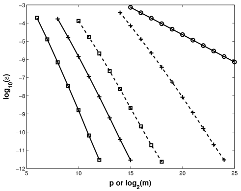
Figure 4: Dependence of the error $\epsilon$ on the truncation order $p$ for the series expansion algorithms, and $\log_{2}m$ for the Lie-Trotter algorithm. The symbols $\boxdot$, $+$ and $\odot$ respectively represent the results for the reflection operator series, the projection operator series and the Lie-Trotter algorithm. Continuous and dashed lines connect series expansion results for $\Delta t=1$ and $\Delta t=\pi$ respectively.

We carried out our tests on a one-dimensional periodic lattice of length $L=128$, with a random initial state $|\psi(0)\rangle$. We quantified the error as the norm of the difference between the simulated and the exact states, i.e. $\epsilon=\big{|}\big{|}|\widetilde{\psi}\rangle-|\psi\rangle\big{|}\big{|}$. We also needed $mp\delta<\epsilon$ to keep the round-off errors under control. That was not possible with 32-bit arithmetic, and we used 64-bit arithmetic.

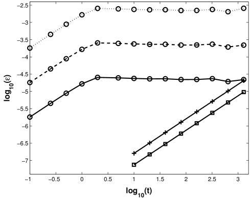
Figure 5: Dependence of the error $\epsilon$ on the evolution time for the series expansion and the Lie-Trotter algorithms. The symbols $\boxdot$, $+$ and $\odot$ respectively represent the results for the reflection operator series (with $p=8,\Delta t=1)$, the projection operator series (with $p=10,\Delta t=1)$, and the Lie-Trotter algorithm (with $\Delta t=0.0001$, $0.001$ and $.01$ values connected by continuous, dashed and dotted lines respectively).

We selected $t=100$ to study the dependence of the error on the evolution step size and the series truncation order. Our results are displayed in Fig.4. For the series expansion algorithms, as expected, we observe that (a) the truncation order $p$ depends linearly on $\log(\epsilon)$, (b) the numerical values are consistent with the bounds in Eqs.(59,74) but the bounds are not very tight, and (c) the reflection operator series converges faster than the projection operator series. For $\Delta t=1$, the coefficients $c_{k}(\Delta t)$ and $r_{k}(\Delta t)$ decrease monotonically, and the series reach a given error $\epsilon$ with a smaller order $p$ compared to the case $\Delta t=\pi$. But in the overall computational complexity, this reduction in $p$ (roughly a factor of 1.6) is more than offset by the increase in $m$ (a factor of $\pi$), and so the choice $\Delta t=\pi$ is slightly more efficient (by roughly a factor of 2). Even larger $\Delta t$ increase the range over which $c_{k}(\Delta t),r_{k}(\Delta t)$ vary, and hence require higher precision arithmetic (i.e. larger $b$). Consequently, it may not be practical to implement such large $\Delta t$.

For the Lie-Trotter algorithm, we find that the error $\epsilon$ is inversely proportional to $m$. As a specific comparison, to make $\epsilon<10^{-5}$, we needed $p>16$ for the projection operator series, $p>11$ for the reflection operator series (both with $\Delta t=\pi$), and $m>2^{21}$ for the Lie-Trotter algorithm. The computational cost $2mp{\cal C}$ of the series expansion algorithms is then of the order $7\times 10^{2}{\cal C}$, which is a huge improvement over the corresponding cost $ml{\cal C}=4\times 10^{6}{\cal C}$ for the Lie-Trotter algorithm. The ratio of the two is consistent with the order of magnitude expectation $(-\epsilon\log\epsilon)$.

To study the growth of the error with the evolution time, we varied the simulation time $t$, while holding $\Delta t$ and $p$ fixed. Our results are illustrated by Fig.5. For the series expansion algorithms, we find that $\epsilon$ is proportional to $t$, implying that the errors of successive time steps additively accumulate, in accordance with Eq.(31). But we also find that for the Lie-Trotter algorithm such additive accumulation of error holds only for $t\lesssim 1$. Beyond that the error saturates with the saturation value proportional to $\Delta t$. This stoppage of error growth for large $t$ indicates cancellations among the errors of different time steps, possibly due to correlations in the periodic evolution beyond the first cycle (period of $\exp(-iH_{i}t)$ is $2\pi$). We note that for $t\gtrsim 1$, we have roughly $m=t/\Delta t\propto t/\epsilon$, and not $m\propto t^{2}/\epsilon$ as per Eq.(3.4).

5 Efficient Simulation of Local Hamiltonian Evolution

We now construct a rapidly converging series expansion for $\exp(-iHt)$, where $H$ is any local efficiently computable Hamiltonian. (The reason for decomposing the Hamiltonian into block-diagonal parts appears later in Section 5.3.) It is well-known that an expansion in terms of the Chebyshev polynomials provides uniform approximation for any bounded function, with fast convergence of the series [25]. We use such an expansion for $\exp(-iHt)$, interpreting all matrix functions as their power series expansions [23].

5.1 Chebyshev Expansion and its Complexity

For any bounded Hamiltonian, its eigenvalue spectrum is within a range $[\lambda_{\rm min},\lambda_{\rm max}]$. With a linear transformation, this range can be mapped to the interval $[-1,1]$ that is the domain of the Chebyshev polynomials $T_{n}(x)=\cos(n\cos^{-1}x)$. Explicitly,

$$e^{-iHt} = e^{-i(\lambda_{\rm max}+\lambda_{\rm min})t/2}e^{-i\tilde{H}\tilde{t}}~{},$$ (81)

$$\tilde{H} = (2H-(\lambda_{\rm max}+\lambda_{\rm min})I)/(\lambda_{\rm max}-\lambda_{\rm min}),$$ (82)

$$\tilde{t} = t(\lambda_{\rm max}-\lambda_{\rm min})/2~{}.$$ (83)

In situations where $\lambda_{\rm min}$ and $\lambda_{\rm max}$ are not exactly known, respectively lower and upper bounds for them can be used. Henceforth, we assume that such a mapping has been carried out and drop the tilde’s on $H$ and $t$ for simplicity.

The Chebyshev expansion gives

$$e^{-iHt}=\sum_{k=0}^{\infty}C_{k}(t)~{}T_{k}(H)~{},$$ (84)

where the expansion coefficients are the Bessel functions:

$$C_{0} = \frac{1}{\pi}\int_{0}^{\pi}e^{-it\cos\theta}d\theta=J_{0}(t)~{},$$ (85)

$$C_{k>0} = \frac{2}{\pi}\int_{0}^{\pi}e^{-it\cos\theta}\cos(k\theta)~{}d\theta=2(-i)^{k}J_{k}(t)~{}.$$ (86)

Note that the Chebyshev polynomials are bounded in $[-1,1]$, and the coefficients $J_{k}(t)=t^{k}/(2^{k}k!)+\ldots$ fall off faster by a factor of $2^{k}$ compared to the corresponding coefficients $t^{k}/k!$ of the Taylor series expansion. This is the well-known advantage of the Chebyshev expansion compared to other series expansions.

For the special case analysed in Section 4.2.1, i.e. $H=I-(R_{1}+R_{2})/2$, $R_{i}^{2}=I$ implies that the spectrum of $H$ is bounded in $[-1,1]$. Then from the recursion relation for the Chebyshev polynomials,

$$T_{k+1}(H)=2H~{}T_{k}(H)-T_{k-1}(H)~{},$$ (87)

it follows that

$$T_{k}\left(-\frac{R_{1}+R_{2}}{2}\right)=\frac{(-1)^{k}}{2}\Big{(}(R_{1}R_{2}\ldots)_{k}+(R_{2}R_{1}\ldots)_{k}\Big{)}.$$ (88)

Thus we reproduce the series expansion obtained in Eq.(67), with the same values for $r_{k}(t)$. Looking at it another way, the partial summation of the reflection operator series for $e^{-iHt}$ converts the Taylor series expansion into a better behaved Chebyshev expansion.

When the Chebyshev expansion in Eq.(84) is truncated at order $p$, its error analysis is identical to that in Section 4.2.2. Choosing $t=m\Delta t$ and $\Delta t=\Theta(1)$, the constraint of Eq.(74) formally provides an efficiently converging series with $p=O(\log(t/\epsilon)/\log(\log(t/\epsilon)))$.

We have noted earlier that reflection operations are the largest evolution steps consistent with unitarity, and their use makes Grover’s algorithm optimal. Then, with $e^{i\pi R/2}=iR$, a good guess for the evolution time step is $\Delta t=\pi$. With this choice, the numerical tests in Section 4.3 indicate that truncating the series at order $p=2\ln(t/\epsilon)/\ln(\ln(t/\epsilon))$ is sufficiently accurate.

A truncated series of the Chebyshev expansion is efficiently evaluated using Clenshaw’s algorithm, based on the recursion relation Eq.(87). One initialises the vectors $|y_{p+1}\rangle=0$, $|y_{p}\rangle=C_{p}|x\rangle$, and then uses the reverse recursion

$$|y_{k}\rangle=C_{k}|x\rangle+2H~{}|y_{k+1}\rangle-|y_{k+2}\rangle~{},$$ (89)

from $k=p-1$ to $k=0$. At the end,

$$\sum_{k=0}^{p}C_{k}T_{k}(H)|x\rangle=(C_{0}|x\rangle+|y_{0}\rangle-|y_{2}\rangle)/2$$ (90)

is obtained using $p$ sparse matrix-vector products involving $H$. The computational complexity of the total evolution is then

$$O(mp{\cal C}_{C})=O\left(t\frac{\log(t/\epsilon)}{\log(\log(t/\epsilon))}{\cal C}_{C}\right)~{},$$ (91)

where ${\cal C}_{C}$ is the computational cost of implementing the recursion of Eq.(89).

5.2 An Alternate Strategy

The Chebyshev expansion coefficients $J_{k}(t)$ are bounded for any value of $t$, unlike their Taylor series counterparts, and rapidly fall off for $k>t$. These properties suggest an alternate evolution algorithm, i.e. evaluate $e^{-iHt}$ at one shot without subdividing the time interval into multiple steps [23]. Of course, this requires the Hamiltonian to be time independent; otherwise, the evolution has to be performed piece-wise over time intervals within which the Hamiltonian is effectively constant.

The error due to truncating the Chebyshev expansion at order $p$ is bounded by

$$\sum_{k=p+1}^{\infty}|C_{k}(t)|\leq\sum_{k=p+1}^{\infty}\frac{t^{k}}{2^{k-1}k!}\leq\frac{t^{p+1}}{2^{p}(p+1)!}\left(1-\frac{t}{2(p+2)}\right)^{-1},$$ (92)

provided the subleading contribution in Eq.(72) can be ignored. The subleading contribution can certainly be neglected for $p>t^{2}/8$, but the bound in Eq.(92) may hold for even smaller values of $p$ due to cancellations among subleading contributions of different terms in the series. Making Eq.(92) smaller than $\epsilon$ requires $p+1>et/2$, and the formal bound is $p=O(t\epsilon^{-2/(et)})=O(t+\log(1/\epsilon))$ for $t>\log(1/\epsilon)$. The resultant computational complexity of the evolution,

$$O(p{\cal C}_{C})=O(t\epsilon^{-2/(et)}{\cal C}_{C})=O((t+\log(1/\epsilon)){\cal C}_{C})~{},$$ (93)

can be comparable to Eq.(91) for values of $\epsilon$ and $t$ that are of practical interest. The extent to which the computational complexity would be enhanced by the need to control subleading contributions can be problem dependent, and needs to be determined numerically [23].

To implement this strategy, the Bessel functions $J_{k}(t)$ upto order $p$ need to be evaluated to $b=\Omega(\log(p/\epsilon))$ bit precision. That can be efficiently accomplished using the recursion relation,

$$J_{k-1}(t)=\frac{2k}{t}J_{k}(t)-J_{k+1}(t)~{},$$ (94)

in descending order [26]. One starts with approximate guesses for $J_{l}(t)$ and $J_{l+1}(t)$, with $l$ slightly larger than $p$, and uses the recursion relation repeatedly to reach $J_{0}(t)$. Then all the values are scaled to the correct normalisation by imposing the constraint $J_{0}(t)+2\sum_{k=1}^{\lceil l/2\rceil}J_{2k}(t)=1$. This procedure to determine the expansion coefficients requires $\Theta(pb^{2})$ computational effort, and so does not alter the overall computational complexity.

5.3 Digital State Implementation

Summation of the series in Eq.(84), truncated to order $p$, requires $p$ executions of the Clenshaw recursion relation, Eq.(89). Multiplication of a vector by a constant, and addition of two vectors, are easily carried out with the digital representation of Section 3.5. Multiplication of the sparse Hamiltonian with a vector, on the other hand, has to be carefully implemented such that quantum parallelism converts its computational complexity from classical $O(N)$ to quantum $O(n)$.

Multiplication by the diagonal elements of the Hamiltonian has a trivial parallel structure. but its parallelisation for the off-diagonal elements of the Hamiltonian needs decomposition of $H$ into parts, with each part consisting of a large number of mutually independent blocks. As mentioned earlier in Section 2.1, such a decomposition can be achieved for any sparse Hamiltonian using an edge-colouring algorithm for the corresponding graph. With $l$ colours, there are $l$ Hamiltonian parts, each containing $O(N/2)$ mutually independent $2\times 2$ blocks. (Note that Hermiticity of the Hamiltonian relates the off-diagonal elements, $H_{j,j+\mu}=H^{*}_{j+\mu,j}$, that are represented by a single edge of the graph.) Evaluating the contribution of each Hamiltonian part in succession, and combining the individual block calculations for each Hamiltonian part with a superposition of their block labels, the total computational effort for Hamiltonian multiplication becomes $O(l\log(N/2))$ times the effort for a single $2\times 2$ block multiplication.

In the digital representation, the $2\times 2$ block multiplication becomes straightforward provided one can swap the $b$-bit register values, i.e.

$$|j\rangle|y_{j}\rangle+|j+\mu\rangle|y_{j+\mu}\rangle\longrightarrow|j\rangle|y_{j+\mu}\rangle+|j+\mu\rangle|y_{j}\rangle~{}.$$ (95)

Such a swap operation can be performed by the reflection operator,

$$S=\sigma_{1}\otimes I^{\otimes b}~{},~{}~{}S^{2}=I~{},$$ (96)

acting on the subspace $\{|j\rangle,|j+\mu\rangle\}\otimes\{|y_{j}\rangle,|y_{j+\mu}\rangle\}$. The swap can be easily undone after the off-diagonal element multiplication for a particular Hamiltonian part $H_{i}$, to use $|y_{j}\rangle$ again for the next Hamiltonian part.

Figure 6: Digital quantum logic circuit for executing the recursion relation of Clenshaw’s algorithm, Eq.(89), to be executed with a uniform superposition over the index $j$. Operations for a single $H_{i}$ containing only $2\times 2$ blocks (labeled by $j,j+\mu_{i}$) are shown. Among the controlled logic gates,

The digital circuit implementation of Eq.(89), for a single Hamiltonian part $H_{i}$, is schematically illustrated in Fig.6. It has computational complexity $O(b^{3})$ arising from evaluation of the Hamiltonian elements; the rest of the linear algebra operations have computational complexity $O(b^{2})$. Including contributions of all the Hamiltonian parts, and the computational effort needed to superpose the index $j$, we thus have the time complexity ${\cal C}_{C}=O(lnb^{3})$. We also point out that the space resources required to put together the full Chebyshev expansion are a fixed number of $n$-bit registers and $O(p)$ $b$-bit registers.

Finally, note that the classical computational complexity for implementing Eq.(89) is ${\cal C}_{C}=O(lNb^{3})$. In our construction based on digital representation for the quantum states, the full quantum advantage that reduces $N$ to $n$ arises from a simple superposition of the quantum state label $j$, and this superposition in turn requires decomposition of the Hamiltonian into block-diagonal parts.

6 Summary and Outlook

We have presented efficient quantum Hamiltonian evolution algorithms belonging to the class P:P, for local efficiently computable Hamiltonians that can be mapped to graphs with bounded degree. Our construction exploits the fact that, the Lie-Trotter evolution formula can be reorganised in terms of reflection operators and Chebyshev expansions (by partially summing up the BCH or the Taylor expansions), so as to be accurate for finite time step size $\Delta t=\Theta(1)$. Specifically, $P^{2}=P$ and $R^{2}=I$ allow easy summation of a large number of terms, while the large spectral gap of $P$ and $R$, due to only two distinct eigenvalues, provides a rapid convergence of the series. The net result is a dramatic exponential gain in the computational error complexity. Our expansions have better convergence properties than previous similar results [8, 24], obtained by successively reducing the Hamiltonian evolution problem to simpler instances. Furthermore, our explicit constructions show how to design practical efficient algorithms, and reveal the physical reasons underlying their efficiency.

The formalism that we have developed has connections to the familiar method for combining exponentials of operators, i.e. the Baker-Campbell-Hausdorff formula. This formula can be partially summed up and simplified for exponentials of projection operators. Several identities for projection operators that are useful in the process are described in the Appendix. In particular, the identity of Eq.(104) may be useful in other applications of the BCH expansion.

Our methods have introduced two concepts that go beyond the specific problem investigated here. One is that unitary time evolution using a large step size can be looked upon as simulation of an effective Hamiltonian. This effective Hamiltonian can be very different from the original Hamiltonian that defined the evolution problem in continuous time, as seen in our analysis of Grover’s algorithm. Such a correspondence between two distinct Hamiltonians that give the same finite time evolution is highly non-trivial, and underlies efficient summation of the BCH expansion. The technique of speeding up simulations by finding appropriate equivalent Hamiltonians can be useful in a variety of problems defined as continuous time evolutions (including adiabatic ones).

The other novel concept we have used is to map non-unitary linear algebra operations to unitary operators using the digital state representation. High precision calculations need a digital representation instead of an analog one. We have introduced such a representation for both the quantum states and operators, that maintains the expectation values of all physical observables. It combines classical reversible logic with equally weighted linear superposition, and is essentially free of the unitarity constraint for quantum states. Such digital implementations can help in construction of class P:P quantum algorithms for many linear algebra problems.

A noteworthy feature of our algorithms is that they do not make direct use of any quantum property other than linear superposition—the constraint of unitary evolution is reduced to an overall normalisation that can be taken care of at the end of the computation and need not be explicitly imposed at intermediate stages of the algorithm. Specifically, the digital representation of quantum states makes linear algebra operations involving action of block-diagonal Hamiltonians on a quantum state extremely simple. The Hamiltonian blocks can be processed in superposition on a quantum computer, while they can be handled by independent processors on a classical parallel computer. Consequently, our algorithms can be used for classical parallel computer simulations of quantum systems, with the same exponential gain in temporal computational error complexity. Of course, classical and quantum simulations will differ in the spatial resources, $N$ classical variables vs. $\log(N)$ quantum components, but the temporal cost will be identical with $\Delta t=\Theta(1)$. In other words, classical and quantum complexities differ only in the cost ${\cal C}$ parametrising the resources required to carry out a sparse matrix-vector product, and the exponential gain in quantum spatial complexity simply arises when this product can be evaluated using superposition of an exponentially large number of blocks.

Appendix A Some Identities for Projection Operators

Let $\{P_{i}\equiv|e_{i}\rangle\langle e_{i}|\}$ be a set of normalised but not necessarily orthogonal projection operators:

$$P_{i}^{2}=P_{i}=P_{i}^{\dagger}~{},~{}~{}Tr(P_{i}P_{j})=|\langle e_{i}|e_{j}\rangle|^{2}\equiv|\lambda_{ij}|^{2}~{}.$$ (97)

Functions of a single projection operator are linear. For instance, the projection operators are easily exponentiated as

$$\exp(i\phi P_{i})=1+(e^{i\phi}-1)P_{i}~{}.$$ (98)

Furthermore, functions of two projection operators reduce to quadratic forms (note that $P_{i}P_{j}P_{i}=|\lambda_{ij}|^{2}P_{i}$). In general, the product of a string of projection operators reduces to an expression where each projection operator appears no more than once, because

$$P_{i_{1}}P_{i_{2}}P_{i_{3}}\ldots P_{i_{n}}P_{i_{1}}=\lambda_{i_{1}i_{2}}\lambda_{i_{2}i_{3}}\ldots\lambda_{i_{n-1}i_{n}}P_{i_{1}}~{}.$$ (99)

Such simplifications reduce any series of projection operators to finite polynomials, and various identities follow.

(A) The operator $(P_{i}-P_{j})^{2}$ has the orthogonal eigenvectors $|e_{i}\rangle\pm|e_{j}\rangle$, with degenerate eigenvalue $1-|\lambda_{ij}|^{2}$. Also the operator $[P_{i},P_{j}]^{2}$ has the same orthogonal eigenvectors, with degenerate eigenvalue $|\lambda_{ij}|^{4}-|\lambda_{ij}|^{2}$. These properties make both these operators proportional to identity in the subspace spanned by $|e_{i}\rangle$ and $|e_{j}\rangle$. In this subspace, therefore, we have $\{P_{i},P_{j}\}=P_{i}+P_{j}-(P_{i}-P_{j})^{2}=P_{i}+P_{j}-1+|\lambda_{ij}|^{2}$, and the identity

$$e^{\pm i\pi P_{i}}e^{\pm i\pi P_{j}} = (1-2P_{i})(1-2P_{j})$$ (100)

$$= -1+2|\lambda_{ij}|^{2}+2[P_{i},P_{j}]$$

$$= -\exp\Big{(}\frac{-2\sin^{-1}(|\lambda_{ij}|)[P_{i},P_{j}]}{\sqrt{|\lambda_{ij}|^{2}-|\lambda_{ij}|^{4}}}\Big{)}~{}.$$

Eqs.(11,13) correspond to the special case of this identity with $\lambda_{ij}=1/\sqrt{N}$.

(B) In the subspace spanned by $|e_{i}\rangle$ and $|e_{j}\rangle$, with a phase choice that makes $\lambda_{ij}\equiv\langle e_{i}|e_{j}\rangle$ real, $|e_{i}\rangle\pm|e_{j}\rangle$ are also the eigenvectors of $P_{i}+P_{j}$, with eigenvalues $1\pm\lambda_{ij}$. The evolution taking $|e_{i}\rangle$ to $|e_{j}\rangle$ can therefore be achieved as

$$\exp(-i(P_{i}+P_{j})T)|e_{i}\rangle = \frac{1}{2}\Big{[}e^{-iT(1+\lambda_{ij})}(|e_{i}\rangle+|e_{j}\rangle)+e^{-iT(1-\lambda_{ij})}(|e_{i}\rangle-|e_{j}\rangle)\Big{]}$$ (101)

$$= \frac{1}{2}e^{-iT(1+\lambda_{ij})}\Big{[}|e_{i}\rangle+|e_{j}\rangle+e^{2iT\lambda_{ij}}(|e_{i}\rangle-|e_{j}\rangle)\Big{]}$$

$$= -ie^{-iT}|e_{j}\rangle,\quad{\rm for}~{}T=\pi/(2\lambda_{ij}).$$

The Farhi-Gutmann search algorithm is the special case of this result with $\lambda_{ij}=1/\sqrt{N}$.

(C) The unitary transformation generated by a projection operator is:

$$e^{i\phi P_{i}}Xe^{-i\phi P_{i}} = (1+(e^{i\phi}-1)P_{i})X(1+(e^{-i\phi}-1)P_{i})$$ (102)

$$= X+i\sin\phi[P_{i},X]+(\cos\phi-1)\big{(}\{P_{i},X\}-2P_{i}XP_{i}\big{)}$$

$$= X+i\sin\phi[P_{i},X]+(\cos\phi-1)[P_{i},[P_{i},X]]~{}.$$

In the Lie algebra language, the adjoint action of an operator is defined as ${\rm ad}Y(X)\equiv[Y,X]$. So the above unitary transformation can be also expressed as

$$e^{i\phi P_{i}}Xe^{-i\phi P_{i}}=e^{i\phi({\rm ad}P_{i})}(X)=\Big{(}1+i\sin\phi({\rm ad}P_{i})+(\cos\phi-1)({\rm ad}P_{i})^{2}\Big{)}(X)~{}.$$ (103)

These expressions can also be derived using the identity

$$[P_{i},[P_{i},[P_{i},X]]]=[P_{i},X]~{}~{}\Longleftrightarrow~{}~{}({\rm ad}P_{i})^{3}(X)={\rm ad}P_{i}(X)~{}.$$ (104)

When $X$ is also a projection operator, further simplification is possible using

$$[P_{i},[P_{i},P_{j}]]=P_{i}+P_{j}-1+|\lambda_{ij}|^{2}(1-2P_{i}),$$ (105)

in the subspace spanned by $|e_{i}\rangle$ and $|e_{j}\rangle$.

(D) When $X$ is a differential operator, interpreting $df/dx\equiv[d/dx,f]$, similar algebra yields

$$e^{i\phi P_{i}}\frac{d(e^{-i\phi P_{i}})}{dx} \equiv e^{i\phi P_{i}}\Big{[}\frac{d}{dx},e^{-i\phi P_{i}}\Big{]}$$ (106)

$$= -iP_{i}\frac{d\phi}{dx}+(e^{-i\phi}-1)\frac{dP_{i}}{dx}+(2-2\cos\phi)P_{i}\frac{dP_{i}}{dx}$$

$$= -iP_{i}\frac{d\phi}{dx}-i\sin\phi\frac{dP_{i}}{dx}+(1-\cos\phi)\Big{[}P_{i},\frac{dP_{i}}{dx}\Big{]}~{}.$$

Note that $P_{i}^{2}=P_{i}$ leads to

$$P_{i}\frac{dP_{i}}{dx}+\frac{dP_{i}}{dx}P_{i}=\frac{dP_{i}}{dx}~{},~{}~{}\Big{[}P_{i},\Big{[}P_{i},\frac{dP_{i}}{dx}\Big{]}\Big{]}=\frac{dP_{i}}{dx}~{}.$$ (107)

(E) The general BCH expansion for combining exponentials of non-commuting operators is an infinite series of nested commutators, and is cumbersome to write down at high orders. But it can be expressed in a compact form using exponentials of adjoint action of the operators [21]:

$$e^{A}e^{B}=\exp\left[A+B-\int_{0}^{1}ds\sum_{n=1}^{\infty}\frac{(1-e^{{\rm ad}A}e^{s~{}{\rm ad}B})^{n}}{n(n+1)}B\right]~{}.$$ (108)

When the operators involved are projection operators, the identities in (C), (D) convert exponentials of adjoint action of the operators to quadratic polynomials, effectively summing up infinite series.

Similar simplification is possible for reflection operators as well, due to the identity $R_{i}=1-2P_{i}$, e.g. $({\rm ad}R_{i})^{3}(X)=4~{}{\rm ad}R_{i}(X)$. The resultant reorganised formula, if necessary with appropriate truncation, can be used as an efficient evolution operator replacing the Lie-Trotter formula. The series in Eq.(54) is an example of such a reorganised BCH expansion.

References

- [1] R.P. Feynman, Simulating physics with computers, Int. J. Theor. Phys. 21 (1982) 467-488.
- [2] S. Lloyd, Universal quantum simulators, Science 273 (1996) 1073-1078.
- [3] D. Aharonov and A. Ta-Shma, Adiabatic quantum state generation and statistical zero knowledge, in Proc. 35th Annual ACM Symp. on Theory of Computing, STOC’03, San Diego, CA, 9-11 June (ACM, New York, 2003), pp.20-29.
- [4] D.W. Berry, G. Ahokas, R. Cleve and B.C. Sanders, Efficient quantum algorithms for simulating sparse Hamiltonians, Comm. Math. Phys. 270 (2007) 359-371.
- [5] N. Wiebe, D. Berry, P. Høyer and B.C. Sanders, Higher order decompositions of ordered operator exponentials, J. Phys. A: Math. Theor. 43 (2010) 065203.
- [6] A.M. Childs and R. Kothari, Simulating sparse Hamiltonians with star decompositions, in Theory of Quantum Computation, Communication and Cryptography (TQC 2010), Lecture Notes in Computer Science 6519 (Springer, 2011), pp.94-103.
- [7] M. Suzuki, Generalized Trotter’s formula and systematic approximants of exponential operators and inner derivations with applications to many-body problems, Comm. Math. Phys. 51 (1976) 183-190.
- [8] D.W. Berry, A.M. Childs, R. Cleve, R. Kothari and R.D. Somma, Exponential improvement in precision for simulating sparse Hamiltonians, in Proc. 46th Annual ACM Symp. on Theory of Computing, STOC’14, New York, NY, 31 May-3 June (ACM, New York, 2014), pp.283-292.
- [9] R.P. Brent and P. Zimmermann, Modern Computer Arithmetic, (Cambridge University Press, 2010).
- [10] S.A. Fenner, An Intuitive Hamiltonian for Quantum Search, arXiv:quant-ph/0004091 (2000).
- [11] J. Roland and N.J. Cerf, Quantum-circuit model of Hamiltonian search algorithms, Phys. Rev. A 68 (2003) 062311.
- [12] A. Patel, Optimisation of quantum evolution algorithms, in Proc. 32nd International Symposium on Lattice Field Theory, New York, NY, 23-28 June 2014, PoS(LATTICE2014)324.
- [13] A.W. Harrow, A. Hassidim and S. Lloyd, Quantum algorithm for solving linear systems of equations, Phys. Rev. Lett. 103 (2009) 150502.
- [14] B.D. Clader, B.C. Jacobs and C.R. Sprouse, Preconditioned quantum linear system algorithm, Phys. Rev. Lett. 110 (2013) 250504.
- [15] D.W. Berry and A.M. Childs, Black-box Hamiltonian simulation and unitary implementation, Quant. Info. Comput. 12 (2012) 29-62.
- [16] H. De Raedt, Product formula algorithms for solving the time-dependent Schrödinger equation, Comp. Phys. Rep. 7 (1987) 1-72.
- [17] J.L. Richardson, Visualizing quantum scattering on the CM-2 supercomputer, Comp. Phys. Comm. 63 (1991) 84-94.
- [18] L.K. Grover, From Schrödinger’s equation to the quantum search algorithm, Pramana 56 (2001) 333-348.
- [19] E. Farhi and S. Gutmann, Analog analogue of a digital quantum computation, Phys. Rev. A 57 (1998) 2403-2406.
- [20] L.K. Grover, A fast quantum mechanical algorithm for database search, in Proc. 28th Annual ACM Symposium on Theory of Computing, STOC’96, Philadelphia, PA, 22-24 May (ACM, New York, 1996), pp.212-219.
- [21] R. Achilles and A. Bonfiglioli, The early proofs of the theorem of Campbell, Baker, Hausdorff, and Dynkin, Arch. Hist. Exact Sci. 66 (2012) 295-358.
- [22] M.A. Nielsen and I.L. Chuang, Quantum Computation and Quantum Information, (Cambridge University Press, 2000), Section 6.2.
- [23] H. Tal-Ezer and R. Kosloff, An accurate and efficient scheme for propagating the time dependent Schrödinger equation, J. Chem. Phys. 81 (1984) 3967-3971.
- [24] D.W. Berry, A.M. Childs, R. Cleve, R. Kothari and R.D. Somma, Simulating Hamiltonian dynamics with a truncated Taylor series, Phys. Rev. Lett. 114 (2015) 090502.
- [25] G.B. Arfken, H.J. Weber and F.E. Harris, Mathematical Methods for Physicists: A Comprehensive Guide, Seventh Edition, (Academic Press, 2011), Chapter 18.4.
- [26] M. Abramowitz and I.A. Stegun (eds.), Handbook of Mathematical Functions: With Formulas, Graphs and Mathematical Tables, (Dover Publications, 1965), Chapter 9.12.