Hierarchical Bond Graph Modelling of Biochemical Networks

Abstract

The bond graph approach to modelling biochemical networks is extended to allow hierarchical construction of complex models from simpler components. This is made possible by representing the simpler components as thermodynamically open systems exchanging mass and energy via ports. A key feature of this approach is that the resultant models are robustly thermodynamically compliant: the thermodynamic compliance is not dependent on precise numerical values of parameters. Moreover, the models are reusable due to the well-defined interface provided by the energy ports.

To extract bond graph model parameters from parameters found in the literature, general and compact formulae are developed to relate free-energy constants and equilibrium constants. The existence and uniqueness of solutions is considered in terms of fundamental properties of stoichiometric matrices.

The approach is illustrated by building a hierarchical bond graph model of glycogenolysis in skeletal muscle.

1 Introduction

A central aim of Systems Biology is to develop computational models for simulation and analysis of complex biological systems. The scale of this challenge is well illustrated by two examples. Firstly, the recent whole-cell model of the pathogenic bacterium mycoplasma genitalium [1] which the authors claim accounts for the dynamics over the cell cycle of every gene product. Even for this relatively simple organism, the model was developed in the form of many submodels describing different cellular processes such as transcription, translation and metabolism; each submodel required a different mathematical description and simulation approach, which were coupled together at simulation time. Secondly the Virtual Physiological Human project [2, 3] “is a concerted effort to explain how each and every component in the body, from the scale of molecules up to organ systems and beyond, works as part of the integrated whole”.

In both examples, a key challenge is to devise modelling strategies and frameworks which not only handle complexity but also unite different aspects of cell biology, for example: cellular metabolism, signalling and electrophysiology. Such systems involve diverse physicochemical domains such as biochemical, chemoelectric and chemomechanical. There is therefore a need for a modelling approach to large multi-domain systems. As discussed below, the bond graph modelling formalism has long been used to model multi-domain engineering systems; and recently it has been applied to components of biochemical systems [4]. The purpose of this paper is extend the modelling of biochemical components to the modelling of biochemical systems by developing a hierarchical bond graph representation of biochemical systems.

As detailed in Gawthrop and Crampin [4], thermodynamic aspects of chemical reactions have a long history in the Physical Chemistry literature. The roles of chemical potential and Gibb’s free energy in biochemical system analysis is described in the textbooks of: Hill [5], Beard and Qian [6] and Keener and Sneyd [7]. Indeed, if a computational model of a biochemical system is to be securely founded in the underlying chemistry, it must fully comply with the fundamental principles of physical chemistry as, for example laid out by Atkins and de Paula [8].

Thermodynamic compliance for a set of rate equations has been considered in some detail by a number of authors [9, 10, 11] allowing this theory to be applied over preexisting models and providing rules to examine new models and ensure that they are constructed to be compliant. However, when rules such as the Haldane constraint are used to constrain a set of numerical parameter values, numerical errors may still destroy thermodynamical compliance. The bond graph approach to modelling dynamical systems is well established - a comprehensive account is given in the textbooks of Gawthrop and Smith [12], Borutzky [13] and Karnopp et al. [14] and a tutorial introduction for control engineers is given by Gawthrop and Bevan [15]. It has been applied to chemical reaction networks by Oster et al. [16, 17] and to chemical reactions by Cellier [18], Greifeneder and Cellier [19] and Gawthrop and Crampin [4]. Thoma and Atlan [20] discuss “osmosis as chemical reaction through a membrane”, LeFèvre et al. [21] model cardiac muscle using the bond graph approach and Diaz-Zuccarini and Pichardo-Almarza [22] discuss the application of bond graphs to biological system in general and muscle models in particular. As illustrated in this paper, the bond graph method provides an alternative approach to ensuring thermodynamic compliance: a biochemical reaction network built out of bond graph components automatically ensures thermodynamic compliance even if numerical values are not correct. In this sense, the bond graph approach is robustly thermodynamically compliant (RTC). Conversely, the discipline imposed by bond graph modelling can alert the modeller to errors and inconsistencies that may otherwise have escaped attention. This is illustrated in this paper in the context of revising a well-established model of glycogenolysis [23].

Thermodynamics distinguishes between: open systems where energy and matter can cross the system boundary; closed systems where energy, but not matter, can cross the system boundary; and isolated systems where neither energy nor matter can cross the system boundary [8]. Living organisms and their subsystems are open as both matter and energy cross the boundaries, thus, mathematical models of living organisms and their subsystems should have explicit formulation as an open system. In the bond graph approach used for this paper, open subsystem models explicitly contain ports through which matter and energy can flow.

The need for a systems level approach has been termed “understanding the parts in terms of the whole” by Cornish-Bowden et al. [24] and the need for mathematical methods to integrate the range of cellular processes has been emphasised by Goncalves et al. [25]. Building such system-level models from components is simplified if preexisting validated models can be reused and combined in new models. A number of standards have been established to distribute re-usable and consistent models of biochemical networks [26], including the mark-up languages SBML [27] and CellML [28], and reporting guidelines such as the Minimum information requested in the annotation of biochemical models (MIRIAM) [29]. A number of models described with SBML and CellML have been published, and many of these are stored within the BioModels Database [30] and the Physiome Repository [31]. More recently developed, SED-ML [32] now allows “simulated experiments” with SBML and CellML models to be described. However, despite the increasing availability of models written using standardised formats, it is still a difficult and complex task to combine such models within a larger system [33, 34].

In the context of a thermodynamically compliant reaction network, model reuse requires that interconnecting models with preexisting thermodynamical compliance produces a model where this property is inherited. As discussed in this paper, bond graph models for open systems contain energy ports which provide the required interconnections thus allowing the models to be combined to produce a higher-level model which is robustly thermodynamically compliant. This form of hierarchical modelling has been used in the bond graph context by Cellier [35] and makes use of bond graph energy ports [18, 14]. As discussed in more detail by Gawthrop and Bevan [15] and later within this paper, the source sensor (SS) bond graph component, introduced by Gawthrop and Smith [36], provides a convenient notation for such energy ports. Because the system components are connected by energy ports, interactions between the components are two-way, thus the distinction between input and output is meaningless and a component’s dynamic properties depend on those components which are connected to it. Thus the analogy with active electronic components (e.g. diodes and transistors) designed to avoid such two-way interactions is not helpful here. Rather, the analogy is with passive electronic components (e.g. resistors and capacitors).

Gawthrop and Crampin [4] also discuss how bond graph models are parameterised such that parameters relating to thermodynamic quantities are clearly demarcated from reaction kinetics. However, this alternative parameterisation leads to an important issue: the parameters required by the bond graph model are not the same as the parameters normally used to describe a biochemical reaction network. Thus parameters must be converted from one form to another. This conversion is not trivial for two reasons: the given parameters must be checked for thermodynamic compliance for a solution to exist, and this solution is not necessarily unique. The problem is solved in this paper and illustrated using a specific example from the literature.

Complex systems may be difficult to comprehend theoretically, and the practical derivation of properties is often tedious. These issues can be overcome to some extent by providing general representations of, and general formulae relating to arbitrarily complex systems. The stoichiometric matrix approach [37, 38] is one such methodology; another approach is provided by van der Schaft et al. [39] who investigate the mathematical structure of balanced chemical reaction networks governed by mass action kinetics and provide a powerful mathematical notation. This paper provides a general representation of an open biochemical reaction network described using bond graphs as well as general formulae based on the stoichiometric matrix [37, 38] approach and on the mathematical structure and notation of van der Schaft et al. [39]. As discussed by Gawthrop and Crampin [4, § 3], the use of the bond graph concept of causality visually and intuitively ties the mathematical concepts of the stoichiometric matrix and its subspaces (representing pathways and conserved moieties) [37, 38] to the actual chemistry underlying the system as represented by the biochemical system bond graph.

One purpose of this paper is to introduce Systems Biologists to the bond graph modelling approach. To this end, a metabolic pathway model from the literature is re-implemented and reexamined from the bond graph point of view. In particular, Lambeth and Kushmerick [23] consider “a computational model for glycogenolysis in skeletal muscle” and provide a detailed thermodynamically consistent model. This model has been further embellished by Vinnakota et al. [40] who also provide a detailed comparison with experimental data. Beard [41, Chapter 7] uses this model as an example for the simulation of complex biochemical cellular systems, and Mosca et al. [42] uses a similar model to examine the interaction of the AKT pathway on metabolism. This paper uses the Lambeth and Kushmerick [23] model as an exemplar of how the bond graph approach can be applied to build a hierarchical model which is RTC.

The outline of the paper is as follows. § 2 discusses the modelling of open thermodynamical systems using bond graphs and the bond graph notion of an energy port; § 2.1 introduces the topic using a simple example, § 2.2 gives the general case and § 2.3 focuses on energy flows. Conversion of kinetic data into the form required for bond graphs is considered in § 3; in particular 3.1 examines the relation between equilibrium constants and free-energy constants and gives a general formula. Existence and uniqueness issues are discussed and an alternative derivation of the Wegscheider conditions is given and § 3.2 discusses the reformulation of enzyme-catalysed reactions. § 4 develops a hierarchical bond graph model based on the well-established model of glycogenolysis by [23] to illustrate the concepts developed in this paper, and § 5 concludes the paper with suggested directions for further work.

A virtual reference environment [43] is available for this paper at https://sourceforge.net/projects/hbgm/.

Notation

Following van der Schaft et al. [39], we use the convenient notation $\text{\bf Exp }X$ to denote the vector whose $i$th element is the exponential of the $i$th element of $X$ and $\text{\bf Ln }X$ to denote the vector whose $i$th element is the natural logarithm of the $i$th element of $X$. van der Schaft et al. [39] also use the element-wise multiplication operator “.”; here, for clarity, we use the equivalent Hadamard or Schur product with symbol “$\circ$”. The Hadamard or Schur operator $\circ$ [44, Sec. 7.3] corresponds to element-wise multiplication of two matrices which have the same dimensions. This is the same as the $.*$ notation within matrix manipulation software. Note that $K\circ X=X\circ K=(\text{diag }K)X=(\text{diag }X)K$, where the notation “$\text{diag }X$” is used for the matrix with elements of $X$ along the diagonal.

2 Closed and Open systems

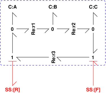
(a) Example: external efforts $\mu_{F}$ and $\mu_{R}$.

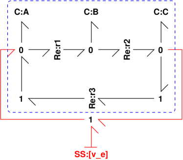
(b) Example: external flow $v_{e}$

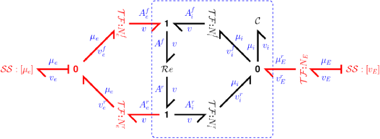
(c) General

Figure 1: Closed & open systems. (a) & (b) Simple examples corresponding to reaction schemes (1) and (2) with imposed concentrations and flows, respectively. The C:A, C:B, and C:C components accumulate the species $A$, $B$ and $C$; and the Re:r1, Re:r2 and Re:r3 represent reactions 1, 2 and 3. The SS:[F], SS:[R] and SS:[v_e] components are the energy ports converting a closed system to an open one. The system inside the dashed box is a closed system; when SS components (representing energy ports) are added the system becomes open. (c) General case. The bond symbols $\rightharpoondown$ correspond to vectors of bonds; $\mathcal{C}$, $\mathcal{R}e$, $\mathcal{SS}$, 0 and 1 symbols correspond to arrays of the associated components; and $\mathcal{TF}$ components represent the intervening junction structure which transmits energy, comprising bonds, junctions and TF components. $\mathcal{SS}:[\mu_{e}]$ represents a vector of energy ports imposing external chemical potentials; $\mathcal{SS}:[v_{E}]$ represents a vector of energy ports imposing external flows. In particular, with respect to (a) & (b), $\mathcal{C}$ corresponds to the species represented by C:A, C:B, and C:C, $\mathcal{R}e$ corresponds to the reactions represented by Re:r1, Re:r2 and Re:r3 and $\mathcal{TF}:N^{f}_{i}$ and $\mathcal{TF}:N^{r}_{i}$ summarise the connections between reactions and species. With respect to (a), $\mathcal{SS}:[\mu_{e}]$ corresponds to SS:[F], SS:[R]; with respect to (b), $\mathcal{SS}:[v_{E}]$ corresponds to SS:[v_e]. $\mathcal{TF}:N^{f}_{e}$ and $\mathcal{TF}:N^{r}_{e}$ summarise the connections between reactions and ports, and $\mathcal{TF}:N_{E}$ between species and ports, in (a) & (b).

This section discusses the modelling of open thermodynamic systems using bond graphs. In particular, it is shown how an otherwise closed system becomes an open system by the addition of energy ports and the standard bond graph components that represent such ports are introduced. A simple motivational example is discussed in § 2.1 and the general case is discussed in § 2.2.

2.1 Simple Example: open and closed systems

As described in Gawthrop and Crampin [4], the reaction scheme:

$$A {\;\xrightleftharpoons{1}\;}B B {\;\xrightleftharpoons{2}\;}C C {\;\xrightleftharpoons{3}\;}A$$ (1)

has the bond graph representation given within the dashed box of Figures 1(a) and 1(b). This is a closed system with respect to the three species $A$, $B$ and $C$, thus the system equilibrium (where the quantities of $A$, $B$ and $C$ are constant) corresponds to zero reaction flows.

In contrast, consider the reaction scheme:

$$A {\;\xrightleftharpoons{1}\;}B B {\;\xrightleftharpoons{2}\;}C C+F {\;\xrightleftharpoons{3}\;}A+R$$ (2)

where the reactants $F$ and $R$ correspond to large external pools with effectively fixed concentrations $X_{f}$ and $X_{r}$. This is represented in Figure 1(a) where two instances of the effort source and flow sensor components, SS:[F] and SS:[R], have been appended to the bond graph. Each SS imposes a chemical potential (effort in bond graph parlance) upon the system and inherits the flow on the corresponding 1 junction. With the sign convention shown, energy flows into the system through SS:[F] and out of the system through SS:[R].

Although there is a net flow of energy into the system, in this particular case there is no net flow of material. The two 1 junctions are connected by an Re component thus the flows are equal.

Further details are given within Gawthrop and Crampin [4] as to how the mass-action kinetics of this closed system can be directly derived from the bond graph:

$${\dot{x}}_{a} =v_{3}-v_{1} {\dot{x}}_{b} =v_{1}-v_{2} {\dot{x}}_{c} =v_{2}-v_{3}$$ (3)

where: $x_{a}$, $x_{b}$ and $x_{c}$ are the amounts of species $A$, $B$ and $C$ in moles; and $v_{1}$, $v_{2}$ and $v_{3}$ are the molar flows associated with reactions 1–3, given by:

$$v_{1} =\kappa_{1}\left(K_{a}x_{a}-K_{b}x_{b}\right) v_{2} =\kappa_{2}\left(K_{b}x_{b}-K_{c}x_{c}\right) v_{3} =\kappa_{3}\left(K_{c}x_{c}-K_{a}x_{a}\right)$$ (4)

These linear equations can be written in the notation of § 1 using the stoichiometric matrix $N$:

$${\dot{X}} =NV V =-\kappa\circ\left(N^{T}K\circ X\right) \text{where }N =\begin{pmatrix}-1&0&1\\ 1&-1&0\\ 0&1&-1\end{pmatrix}$$ (5)

with associated mass and flow vectors, and coefficient matrices:

$$X =\begin{pmatrix}x_{a}\\ x_{b}\\ x_{c}\end{pmatrix} V =\begin{pmatrix}v_{1}\\ v_{2}\\ v_{3}\end{pmatrix} \kappa =\begin{pmatrix}\kappa_{1}\\ \kappa_{2}\\ \kappa_{3}\end{pmatrix} K =\begin{pmatrix}K_{a}\\ K_{b}\\ K_{c}\end{pmatrix}$$ (6)

The open system given by the reaction scheme (2) and the bond graph of Figure 1(a) is given by Equations (3) but the equation for $v_{3}$ of Equations (4) is replaced by:

$$v_{3}=\kappa_{1}\left(K_{f}x_{f}K_{c}x_{c}-K_{r}x_{r}K_{a}x_{a}\right)$$ (7)

The simple linear expression (5) is also no longer applicable, but as discussed in § 2.2 it can be replaced in general terms by:

$${\dot{X}}_{i} =N_{i}V V =\kappa\circ\left(\text{\bf Exp }{N^{f}}^{T}\text{\bf Ln }K\circ X-\text{\bf Exp }{N^{r}}^{T}\text{\bf Ln }K\circ X\right) \text{where }N_{i} =N^{r}_{i}-N^{f}_{i}$$ (8)

and where

$$X =\begin{pmatrix}x_{a}\\ x_{b}\\ x_{c}\\ x_{f}\\ x_{r}\end{pmatrix} K =\begin{pmatrix}K_{a}\\ K_{b}\\ K_{c}\\ K_{f}\\ K_{r}\end{pmatrix} N^{f} =\begin{pmatrix}N^{f}_{i}\\ N^{f}_{e}\end{pmatrix} N^{r} =\begin{pmatrix}N^{r}_{i}\\ N^{r}_{e}\end{pmatrix}$$ (9)

$$N^{f}_{i} =\begin{pmatrix}1&0&0\\ 0&1&0\\ 0&0&1\end{pmatrix} N^{r}_{i} =\begin{pmatrix}0&0&1\\ 1&0&0\\ 0&1&0\end{pmatrix} N^{f}_{e} =\begin{pmatrix}0&0&1\\ 0&0&0\end{pmatrix} N^{r}_{e} =\begin{pmatrix}0&0&0\\ 0&0&1\end{pmatrix}$$ (10)

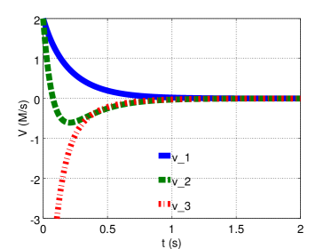
(a) Closed system: $V$

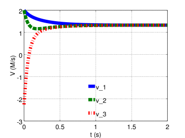
(b) Open system: $V$

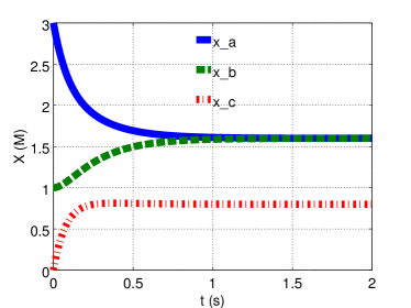
(c) Closed system: $X$

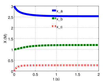
(d) Open system: $X$

Figure 2: Simulation of closed & open systems. The parameters are arbitrarily chosen as: $K_{a}=K_{b}=1$, $K_{c}=K_{f}=2$, $K_{r}=0.25$, $X_{f}=X_{r}=1$, $\kappa_{1}=1$, $\kappa_{2}=2$ & $\kappa_{3}=3$. (a) As this is a closed system, the three reaction flows $v_{1}\dots v_{3}$ become zero as time increases. (b) As this is an open system, the three reaction flows $v_{1}\dots v_{3}$ do not become zero as the system has an external driver. However, as the states become constant, the three flows become equal. (c) Although the closed system flows become zero the states do not, as the system has a conserved moiety: the three states have a constant sum $x_{a}+x_{b}+x_{c}=4$. (d) The three states tend to different values to those in (c); but the moiety is still conserved.

A simulation of this simple example is shown in Figure 2 in order to emphasise the main distinctions between open and closed systems.

2.2 General case

Figure 1(c) is a generalisation of Figures 1(a) and 1(b), giving a schematic representation of the structure for an open system. With reference to Figure 1(c), the five $\mathcal{TF}$ components represent the five flow transformations:

$$v^{f}_{i} =N^{f}_{i}v v^{r}_{i} =N^{r}_{i}v v^{f}_{e} =N^{f}_{e}v v^{r}_{e} =N^{r}_{e}v v^{r}_{E} =N_{E}v_{E}$$ (11)

and thus the five matrices $N^{f}_{i}$, $N^{r}_{i}$, $N^{f}_{e}$, $N^{r}_{e}$ & $N_{E}$ define the stoichiometry of the chemical network.

As emphasised by Gawthrop and Crampin [4] - bonds, TF components and junctions all transport, but do not create or destroy, chemical energy. It follows from this that:

$${v}^{T}A^{f}_{i} ={v^{f}_{i}}^{T}\mu_{i} {v}^{T}A^{r}_{i} ={v^{r}_{i}}^{T}\mu_{i} {v}^{T}A^{f}_{e} ={v^{f}_{e}}^{T}\mu_{e} {v}^{T}A^{r}_{e} ={v^{r}_{e}}^{T}\mu_{e}$$ (12)

Using equations (11), equations (12) become:

$${v}^{T}A^{f}_{i} ={v}^{T}{N^{f}_{i}}^{T}\mu_{i} {v}^{T}A^{r}_{i} ={v}^{T}{N^{r}_{i}}^{T}\mu_{i} {v}^{T}A^{f}_{e} ={v}^{T}{N^{f}_{e}}^{T}\mu_{e} {v}^{T}A^{r}_{e} ={v}^{T}{N^{r}_{e}}^{T}\mu_{e}$$ (13)

As the equations (13) must be true for all $v$, it follows that the affinities $A$ can be expressed in terms of chemical potential $\mu$ as:

$$A^{f}_{i} ={N^{f}_{i}}^{T}\mu_{i} A^{r}_{i} ={N^{r}_{i}}^{T}\mu_{i} A^{f}_{e} ={N^{f}_{e}}^{T}\mu_{e} A^{r}_{e} ={N^{r}_{e}}^{T}\mu_{e} \mu_{E} ={N_{E}}^{T}\mu_{i}$$ (14)

The fact that energy conservation implies Equation (14) is discussed by Cellier [18].

With the notation given in § 1, the Marcelin formula for reaction flows (used by Gawthrop and Crampin [4, Eqn. (2.6)] for the scalar case) may be written as:

$$V =\kappa\circ\left(V_{0}^{+}-V_{0}^{-}\right)+N_{E}v_{E} \text{where }V_{0}^{+} =\text{\bf Exp }{\frac{A^{f}}{RT}} \text{and }V_{0}^{-} =\text{\bf Exp }{\frac{A^{r}}{RT}}$$ (15)

Similarly, the formula for chemical potential $\mu$ of Gawthrop and Crampin [4, Eqn. (2.3)] in terms of the vector $K_{i}$ of free-energy constants is given by:

$$\mu_{i} =RT\text{\bf Ln }K_{i}\circ X_{i} \text{where }K_{i} =\text{\bf Exp }\frac{\mu_{i}^{0}}{RT}$$ (16)

where $\mu_{i}^{0}$ is the vector of standard chemical potentials for the internal species. It is also convenient to re-express the external chemical potentials $\mu_{e}$ as $\mu_{e}=RT\text{\bf Ln }K_{e}\circ X_{e}$. Combining Equations (15)– (16), the reaction flows $V$ are given by:

$$V =\boldsymbol{\kappa}\left(V^{+}_{0}-V^{-}_{0}\right)+V^{E} \text{where }V^{+}_{0} =\text{\bf Exp }{N^{f}}^{T}\text{\bf Ln }K\circ X V^{-}_{0} =\text{\bf Exp }{N^{r}}^{T}\text{\bf Ln }K\circ X$$ (17)

where the composite stoichiometric matrices $N^{f}$ and $N^{r}$, the composite state $X$ and the vector of free-energy constants $K$ are given by:

$$N^{f} =\begin{pmatrix}N_{i}^{f}\\ N_{e}^{f}\end{pmatrix} N^{r} =\begin{pmatrix}N_{i}^{r}\\ N_{e}^{r}\end{pmatrix} X =\begin{pmatrix}X\\ X_{e}\end{pmatrix} K =\begin{pmatrix}K_{i}\\ K_{e}\end{pmatrix}$$ (18)

In the context of the simple example shown in Figure 1(a) it can be verified that substituting the stoichiometric matrices of Equation (9) into Equation (17) leads to Equations (3) and (4). Equation (17) expresses the forward and reverse reaction flows $V^{+}_{0}$ and $V^{-}_{0}$ in terms of species: amounts $X$ and free-energy constants $K$. It is helpful to reexpress $V^{+}_{0}$ and $V^{-}_{0}$ in terms of quantities related to reactions. In particular:

$$V^{+}_{0} =K^{f}\circ X^{f} \text{where }K^{f} =\text{\bf Exp }{N^{f}}^{T}\text{\bf Ln }K \text{ and }X^{f} =\text{\bf Exp }{N^{f}}^{T}\text{\bf Ln }X$$ (19)

$$V^{-}_{0} =K^{r}\circ X^{r} \text{where }K^{r} =\text{\bf Exp }{N^{r}}^{T}\text{\bf Ln }K \text{ and }X^{r} =\text{\bf Exp }{N^{r}}^{T}\text{\bf Ln }X$$ (20)

In the context of the simple example of Figure 1(a)

$${N^{f}}^{T} =\begin{pmatrix}1&0&0&0&0\\ 0&1&0&0&0\\ 0&0&1&1&0\end{pmatrix} {N^{r}}^{T} =\begin{pmatrix}0&1&0&0&0\\ 0&0&1&0&0\\ 1&0&0&0&1\end{pmatrix}$$ (21)

hence

$$K^{f} =\begin{pmatrix}K_{a}\\ K_{b}\\ K_{c}K_{f}\end{pmatrix} K^{r} =\begin{pmatrix}K_{b}\\ K_{c}\\ K_{a}K_{r}\end{pmatrix} X^{f} =\begin{pmatrix}x_{a}\\ x_{b}\\ x_{c}x_{f}\end{pmatrix} X^{r} =\begin{pmatrix}x_{b}\\ x_{c}\\ x_{a}x_{r}\end{pmatrix}$$ (22)

2.3 Energy flow

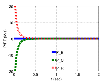
(a) Closed system

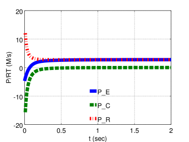
(b) Open system

Figure 3: Energy flows for the system illustrated in Figure 1(a) and simulated in Figure 2: $P_{E}$ is the external energy flowing into the system, $P_{C}$ is the energy flowing into the three C components, and $P_{R}$ is the energy flowing into (and dissipated by) the three Re components. (a) There is no external energy source in the closed system so $P_{E}=0$. Conservation of energy gives $P_{C}+P_{R}=0$: the energy flowing out of the C components is dissipated in the Re components. (b) There is an external energy source in the open system with $\mu_{e}=RT\text{\bf Ln }K_{e}$. Initially, energy flows out of the the open system but, in the steady state, the energy into the system is balanced by the energy dissipated in the Re components and the energy flow into the C components becomes zero.

With reference to Figure 1(c): the bonds ($\rightharpoondown$) and transformers ($\mathcal{TF}$) transmit, but do not create or destroy, chemical energy; the $\mathcal{C}$ components store, but do not create or destroy, chemical energy; the reactions ($\mathcal{R}e$) dissipate, but do not store, chemical energy; and the ports ($\mathcal{SS}$) transmit chemical energy in and out of the system.

The energy dissipated within the Re components represented by $\mathcal{R}e$ is:

$$P_{R} =\sum_{j=1}^{n_{v}}\left(v_{j}A^{f}_{j}-v_{j}A^{r}_{j}\right)=V^{T}A \text{where }A =A^{f}-A^{r}$$ (23)

Using Equations (14), the affinity $A_{i}$ can be rewritten as:

$$A_{i}=A_{i}^{f}-A_{i}^{r}=\left({N_{i}^{f}}^{T}-{N_{i}^{r}}^{T}\right)\mu_{i}=-N_{i}^{T}\mu_{i}=-N_{i}^{T}RT\ln\boldsymbol{K}_{i}X_{i}$$ (24)

Similarly and $A_{e}$ and $A$ can be rewritten as:

$$A_{e} =-N_{e}^{T}\mu_{e}=-N_{e}^{T}RT\ln\boldsymbol{K}_{e}X_{e} \text{and }A =-N^{T}\mu=-N^{T}RT\ln\boldsymbol{K}X$$ (25)

Hence naming the external energy flow into the system as $P_{E}$ and the energy flow into the C components as $P_{C}$ it follows that:

$$P_{E} =RTV^{T}N_{e}^{T}\text{\bf Ln }K_{e}\circ X_{e}$$ (26)

$$P_{C} =RTV^{T}N_{i}^{T}\text{\bf Ln }K_{i}\circ X_{i}$$ (27)

$$\text{and }P_{R} =RTV^{T}N^{T}\text{\bf Ln }K\circ X$$ (28)

These three equations imply energy conservation:

$$P_{E}=P_{C}+P_{R}$$ (29)

Figure 3 is based on data corresponding to the simulations of Figure 2 and illustrates these equations for both closed (no external energy source) and open systems.

3 Conversion of kinetic data

For the bond graph formulation of this paper to be widely applicable, it is necessary to develop a framework for converting kinetic data from the conventional form used with enzyme modelling into the parameters required by the bond graph formulation.

As an example of the issues involved, the reaction $A{\;\xrightleftharpoons{}\;}B$ has a single equilibrium constant $K_{eq}$, whereas the bond graph formulation uses the two thermodynamic constants $K_{a}$ and $K_{b}$. In this case, $K_{eq}=\dfrac{K_{a}}{K_{b}}$, thus it follows that deriving $K_{a}$ and $K_{b}$ from $K_{eq}$ does not have a unique solution. Similarly, the reaction $A{\;\xrightleftharpoons{}\;}B{\;\xrightleftharpoons{}\;}C{\;\xrightleftharpoons{}\;}A$ of Equation (1) has three equilibrium constants. In this case, the solution for $K_{a}$, $K_{b}$ and $K_{c}$ does not exist unless the product of the three equilibrium constants is unity (detailed balance). In § 3.1 a derivation of the formulae that convert equilibrium constants to thermodynamic constants for arbitrary networks of reactions is shown. The solution fully accounts for the potential of such existence and uniqueness issues.

Enzyme-catalysed reactions are commonly represented using Michaelis-Menten kinetics [45]. It should be noted that when a reaction is assumed to be irreversible, the associated Michaelis-Menten kinetics fail to satisfy thermodynamical compliance. For this reason, Michaelis-Menten like kinetics which are thermodynamically compliant have been developed [9, 10, 11]. Section 33.2 focuses on the enzyme-catalysed reaction formulation of Gawthrop and Crampin [4, §5(a)] and compares it to previously developed methods.

In the Supplementary Material, this model is shown to be the same as the as the direct binding modular rate law of Liebermeister et al. [11] in §A.2A.4, compared with the common modular rate law of Liebermeister et al. [11] in §A.2A.5 and compared with the the computational model of Lambeth and Kushmerick [23] in §A.2A.6. As well as the equilibrium constant, mass-action reaction kinetics also require a rate constant. The corresponding conversion to bond graph form is discussed in §A.2A.3 of the Supplementary Material.

3.1 Equilibrium Constants and Free-energy Constants

With the notation given in § 1, the scalar de Donder formula [46, Equation(11)] for the ratio ${\tilde{V}}_{0}$ of the forward $V_{0}^{+}$ and backward $V_{0}^{-}$ reaction rates of Equation (15) can be written in vector form as:

$${\tilde{V}}_{0} =\text{\bf Exp }\frac{A}{RT} \text{or }\text{\bf Ln }{\tilde{V}}_{0} =\frac{A}{RT}$$ (30)

where $A=A^{f}-A^{r}$ In a similar fashion to (19) & (20) and using Equation (25), Equation (30) can be written as:

$${\tilde{V}}_{0} =K^{v}\circ X^{v} \text{where }K^{v} =\text{\bf Exp }\left({-N}^{T}\text{\bf Ln }K\right) \text{ and }X^{v} =\text{\bf Exp }\left({-N}^{T}\text{\bf Ln }X\right)$$ (31)

Substituting Equation (31) into Equation (30) gives the alternative expression for the affinity $A$:

$$A=RT\left(\text{\bf Ln }K^{v}\circ X^{v}\right)=RT\left(\text{\bf Ln }K^{v}+\text{\bf Ln }X^{v}\right)$$ (32)

In the context of the simple example of Figure 1(a):

$${-N}^{T} =\begin{pmatrix}1&-1&0&0&0\\ 0&1&-1&0&0\\ -1&0&1&1&-1\end{pmatrix} K^{v} =\begin{pmatrix}\frac{K_{a}}{K_{b}}\\ \frac{K_{b}}{K_{c}}\\ \frac{K_{c}K_{f}}{K_{a}K_{r}}\end{pmatrix} X^{v} =\begin{pmatrix}\frac{X_{a}}{X_{b}}\\ \frac{X_{b}}{X_{c}}\\ \frac{X_{c}X_{f}}{X_{a}X_{r}}\end{pmatrix}$$ (33)

As discussed by [7, Eq 1.15], the equilibrium constant of a reaction is given by $\exp\frac{\Delta G_{0}}{RT}$. Combining all reactions, the vector $K^{eq}$ of equilibrium constants is thus:

$$K^{eq}=\text{\bf Exp }\frac{\Delta G_{0}}{RT}=\text{\bf Exp }\frac{A_{0}}{RT}$$ (34)

where the subscript $0$ indicates the reference state where $X$ is unity. Hence, substituting unit $X$ into Equation (31), Equation (34) becomes:

$$K^{eq}=K^{v}=\text{\bf Exp }\left({-N}^{T}\text{\bf Ln }K\right)$$ (35)

Equilibrium corresponds to $A=0$ or ${\tilde{V}}_{0}=1_{n_{v}\times 1}$ hence, using Equation (31), equilibrium also corresponds to:

$$X^{v} =X^{eq} \text{where }K^{eq}X^{eq}=1_{n_{v}\times 1}$$ (36)

Equation (35) gives an explicit expression for the vector $K^{eq}$, containing $n_{V}$ reaction equilibrium constants, in terms of the vector $K$ which contains the free energy constants of $n_{X}$ species.

However, the transposed stoichiometric matrix $N^{T}$ is not normally full rank, and so it is not possible to directly use Equation (35) to give $K$ in terms of $K^{eq}$. But, as is now demonstrated, the left and right null space matrices (as used to detect conserved moieties and flux pathways [37, 38]) lead to the solutions (if any) of Equation (35) giving $K$ in terms of $K^{eq}$.

The $n_{v}\times n_{R}$ right null-space matrix $R$ of $N$ has the property that:

$$NR =0 \text{or }R^{T}N^{T} =0$$ (37)

This matrix is used in stoichiometric analysis to analyse metabolic pathways [37, 38]. Here, it is reused to examine thermodynamic constraints. Multiplying equation (35) by $R^{T}$ gives:

$$R^{T}\text{\bf Ln }K^{eq} =0$$ (38)

Equation (38) defines a thermodynamic constraint on the equilibrium constants, and is a form of Wegscheider condition [11, 45].

Assuming that the constraint (38) holds, the Moore-Penrose generalised inverse [44, §6.1] $N^{\dagger}$ of $-N^{T}$ can be used to find a solution for $K$. In particular:

$$\text{\bf Ln }K_{0} =N^{\dagger}\text{\bf Ln }K^{eq} \text{or }K_{0} =\text{\bf Exp }(N^{\dagger}\text{\bf Ln }K^{eq})$$ (39)

In general, the solution of Equation (39), $K=K_{0}$, is not the only value of $K$ satisfying Equation (35). The $n_{G}\times n_{X}$ left null-space matrix $G$ (as used to detect conserved moieties [37, 38]) has the property that:

$$GN =0 \text{or }N^{T}G^{T} =0$$ (40)

Hence a family of solutions of Equation (35) is given by:

$$\text{\bf Ln }K =\text{\bf Ln }K_{0}+\text{\bf Ln }K_{1}=\text{\bf Ln }K_{0}{\circ}K_{1}$$ (41)

$$\text{where }\text{\bf Ln }K_{1} =G^{T}\text{\bf Ln }\boldsymbol{k}^{c}_{1}$$ (42)

$$\text{or }K_{1} =\text{\bf Exp }(G^{T}\text{\bf Ln }\boldsymbol{k}^{c}_{1})$$ (43)

where $\boldsymbol{k}^{c}_{1}$ is an arbitrary $n_{G}\times 1$ vector. Equation (41) can be rewritten as:

$$K =K_{0}{\circ}K_{1}$$ (44)

Finally, we show that the affinity $A$ is also unaffected by the choice of $\boldsymbol{k}^{c}_{1}$. From Equations (25) and (41)–(44) it follows that:

$$A =-N^{T}RT\text{\bf Ln }(K{\circ}X)=RT\text{\bf Ln }K_{0}{\circ}K_{1}{\circ}X=RT(-N^{T}\text{\bf Ln }K_{0}-N^{T}\text{\bf Ln }K_{1}-N^{T}\text{\bf Ln }X)$$ (45)

Using (40) & (43), $N^{T}\text{\bf Ln }K_{1}=0$. Hence $A$ is unaffected by the choice of $\boldsymbol{k}^{c}_{1}$. It follows that the energy-based analysis of § 2.3 is also unaffected by the choice of $\boldsymbol{k}^{c}_{1}$.

Example

The closed system embedded in Figure 1(a) has stoichiometric matrix $N$, and left and right null space matrices $G$ and $R$ given by:

$$N =N_{i}=\begin{pmatrix}-1&0&1\\ 1&-1&0\\ 0&1&-1\end{pmatrix} G =\begin{pmatrix}1&1&1\end{pmatrix} R =\begin{pmatrix}1\\ 1\\ 1\end{pmatrix}$$ (46)

With this value of $R$, Equation (38) implies that:

$$\ln K^{eq}_{1}+\ln K^{eq}_{2}+\ln K^{eq}_{1} =0 \text{or }K^{eq}_{1}K^{eq}_{3}K^{eq}_{3} =1$$ (47)

This is the standard “detailed balance” result applied to a three-reaction loop [7, §1.3].

Taking the example further, suppose $K^{eq}=(1,\,0.5,\,2)^{T}$ (which satisfies Equation (47)). Then using the GNU Octave implementation pinv to calculate the pseudo inverse for Equation (39) gives $K_{0}=(0.79370,\,0.79370,\,1.58740)^{T}$. Noting that $n_{G}=1$, $k_{1}$ is a scalar and may be chosen as $k_{1}=1/0.79370$ leading to $K=(1,\,1,\,2)^{T}$.

In contrast, the open system of Figure 1(a) has stoichiometric matrix $N$, and left and right null space matrices $G$ and $R$ are given by

$$N =\begin{pmatrix}-1&0&1\\ 1&-1&0\\ 0&1&-1\\ 0&0&-1\\ 0&0&1\\ \end{pmatrix} G =\begin{pmatrix}1&1&1&0&0\\ 0&0&0&1&1\end{pmatrix} R =0$$ (48)

Because $R=0$, the constraint (38) holds for any choice of the three elements of $K^{eq}$. For example, suppose $K^{eq}=(1,\,0.5,\,16)^{T}$, then using the GNU Octave implementation pinv for the pseudo inverse, Equation (39) gives $K_{0}=(0.79370,\,0.79370,\,1.58740,\,2.82843,\,0.35355)^{T}$. Noting that $n_{G}=2$, $k_{1}$ has two elements and may be chosen, for example, as $k_{1}=(1/0.79370,\,2/1.58740$ leading to $K=(1,\,1,\,2,\,2,\,0.25)^{T}$.

3.2 Enzyme Catalysed Reactions

The kinetics of enzyme catalysed reactions are usually described by versions of the Michaelis-Menten equations; see, for example, Klipp et al. [45, §2.1] or Keener and Sneyd [7, §1.4]. The key issue is that the equations should be thermodynamically compliant [11].

Gawthrop and Crampin [4, §5(a)] give one possible formulation of the kinetics for enzyme catalysed reactions that is guaranteed to be thermodynamically compliant:

$$v =\bar{\kappa}\frac{K_{e}e_{0}}{1+\frac{\sigma_{v}}{k_{v}}}\delta_{v} \text{ where }\sigma_{v}=\frac{\kappa_{1}V_{0}^{+}+\kappa_{2}V_{0}^{-}}{\kappa_{1}+\kappa_{2}}$$ (49)

where $V_{0}^{+}$ and $V_{0}^{-}$ are given by Equation (15), $e_{0}$ is the total enzyme concentration, and $\kappa_{1}$ and $\kappa_{2}$ are reaction constants for the reactions relating substrate to complex and complex to product respectively. $k_{v}$ is a constant related to the enzyme/complex equilibrium. As is now shown this formulation can be rewritten as a reversible Michaelis-Menten equation. Defining:

$$\rho_{v}=\frac{\kappa_{2}}{\kappa_{1}+\kappa_{2}}\text{ gives }\sigma_{v}=(1-\rho_{v})V_{0}^{+}+\rho_{v}V_{0}^{-}$$ (50)

With reference to Equation (49), define:

$$v_{max}^{+}=\lim_{V_{0}^{+}\rightarrow\infty}v=\frac{v_{max}}{1-\rho_{v}}\;\text{ and }v_{max}^{-}=\lim_{V_{0}^{-}\rightarrow\infty}v=\frac{v_{max}}{\rho_{v}}\;\text{ where }v_{max}=\bar{\kappa}k_{c}e_{0}$$ (51)

then Equation (49) can be rewritten as:

$$v=\frac{v_{max}^{+}\frac{V_{0}^{+}}{k_{v}^{+}}-v_{max}^{-}\frac{V_{0}^{-}}{k_{v}^{-}}}{1+\frac{V_{0}^{+}}{k_{v}^{+}}+\frac{V_{0}^{-}}{k_{v}^{-}}}\text{ where }k_{v}^{+}=\frac{k_{v}}{(1-\rho_{v})}\;,k_{v}^{-}=\frac{k_{v}}{\rho_{v}}$$ (52)

Combining Equations (51) and (52):

$$v=\frac{v_{max}}{k_{v}}\frac{V_{0}^{+}-V_{0}^{-}}{1+\frac{1}{k_{v}}\left(\left(1-\rho_{v}\right)V_{0}^{+}+\rho_{v}V_{0}^{-}\right)}=\frac{v_{max}\left(V_{0}^{+}-V_{0}^{-}\right)}{k_{v}+\left(1-\rho_{v}\right)V_{0}^{+}+\rho_{v}V_{0}^{-}}$$ (53)

Remarks

1. Equation (53) explicitly shows that this particular form of the reversible Michaelis-Menten equation has three parameters: $v_{max}$, $k_{v}$ and $\rho_{v}$.

2. When $\rho_{v}=0$, Equation (53) becomes the irreversible Michaelis-Menten equation but with the addition of the $V_{0}^{-}$ term to give reversibility.

3. Using Equation (51), the two parameters $v_{max}$ and $\rho_{v}$ can be computed from $v_{max}^{+}$ and $v_{max}^{-}$ as:

   $$\rho_{v}=\frac{\frac{v_{max}^{+}}{v_{max}^{-}}}{1+\frac{v_{max}^{+}}{v_{max}^{-}}}=\frac{v_{max}^{+}}{v_{max}^{+}+v_{max}^{-}}\text{ and }v_{max}=\frac{v_{max}^{+}v_{max}^{-}}{v_{max}^{+}+v_{max}^{-}}$$ (54)

4. Using Equation (52), the third parameter $k_{v}$ can be computed from:

   $$k_{v}=\left(1-\rho_{v}\right)k_{v}^{+}=\rho_{v}k_{v}^{-}$$ (55)

5. Note that the Haldane equation $K_{eq}=\dfrac{v_{max}^{+}k_{v}^{-}}{v_{max}^{-}k_{v}^{+}}$ is automatically satisfied by Equation (53).

6. In the limit as $k_{v}\rightarrow\infty$, Equation (53) becomes the mass-action flow [4, Equation (2.6) ]:

   $$v=\kappa\left(V_{0}^{+}-V_{0}^{-}\right)\text{ where }\kappa=\frac{v_{max}}{k_{v}}$$ (56)

4 Hierarchical modelling

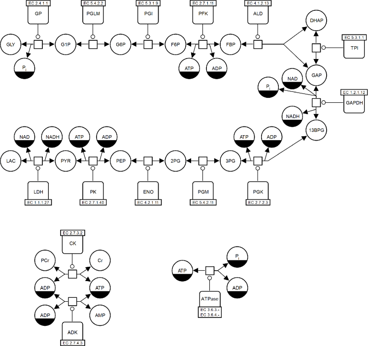
Figure 4: The simplified glycolytic pathway as described by Lambeth and Kushmerick [23, Figure 1]. Reactions/enzymes: GP, glycogen phosphorylase; PGLM, phosphoglucomutase; PGI, phosphoglucose isomerase; PFK, phosphofructo kinase; ALD, aldolase; TPI, triose phosphate isomerase; GAPDH, glyceraldehyde 3-phosphate dehydrogenase; PGK, phosphoglycerate kinase; PGM, phosphoglycerate mutase; ENO, enolase; PK, pyruvate kinase; LDH, lactate dehydrogenase; CK, creatine kinase; ADK, adenylate kinase; ATPase, ATPases. Metabolites: GLY, glycogen; P_i, inorganic phosphate; G1P, glucose-1-phosphate; G6P, glucose-6-phosphate; F6P, fructose-6-phosphate; ATP, adenosine triphosphate; ADP, adenosine diphosphate; FBP, fructose-1,6-biphosphate; DHAP, dihydroxyacetone phosphate; GAP, glyceraldehyde 3-phosphate; NAD, oxidised nicotinamide adenine dinucleotide; NADH, reduced NAD; 13BPG, 1,3-bisphosphoglycerate; 3PG, 3-phosphoglycerate; 2PG, 2-phosphoglycerate; PEP, phosphoenolpyruvic acid; PYR, pyruvate; LAC, lactate; PCr, phosphocreatine; Cr, creatine; AMP, adenosine monophosphate. Enzyme commission (EC) numbers are shown.

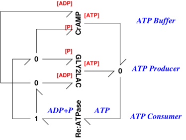
(a) LamKus02

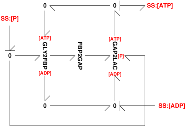
(b) GLY2LAC

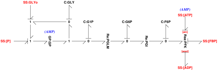
(c) GLY2FBP

(d) FBP2GAP

(e) GP

Figure 5: Hierarchical Bond Graph Model. (a) As discussed in the text, LamKus02 represents the top-level model of the system in Figure 4. (b) GLY2LAC represents one of the three submodels in (a). (c)&(d) GLY2FBP&FBP2GAP represent two of the three submodels in (b). (e) The reaction $GP$ has two parallel reactions $GPa$ and $GPb$.

The bond graph representation for open systems detailed in §2 Figure 1, with the $\mathcal{SS}$ ports to connect systems, provides a basis to construct hierarchical models of biochemical systems that are robustly thermodynamically compliant. This approach is illustrated using a well-established model from the literature: “A Computational Model for Glycogenolysis in Skeletal Muscle” presented by Lambeth and Kushmerick [23]. Although the model has been further embellished by Vinnakota et al. [40] and used as an example in the book of Beard [41], we use information and parameters from the original model as a basis for the discussion in this paper.

Figure 4 shows the simplified glycolysis pathway from Lambeth and Kushmerick [23, Figure 1] using Systems Biology Graphical Notation (SBGN) [47]. There are many ways to subdivide this system to create a hierarchical model. Here, we have chosen to divide the system into three conceptual modules:

1. The primary glycolytic reaction chain leading from glycogen ($GLY$) to lactate ($LAC$) which converts adenosine diphosphate ($ADP$) and inorganic phosphate ($P$) into adenosine triphosphate ($ATP$) making use of the energy stored in glycogen. This module is a producer of ATP.

2. The pair of reactions catalysed by creatine kinase $CK$ and adenylate kinase $ADK$ involving creatine ($Cr$), phosphocreatine ($PCr$) and adenosine monophosphate ($AMP$) as well as $ATP$ and $ADP$. This module is a buffer of ATP.

3. The reactions catalysed by numerous ATPases ($ATPase$; for a more comprehensive description see Lambeth and Kushmerick [23]) which convert $ATP$ into $ADP$ and $P$, and use the released energy to perform work. This module is a consumer of ATP.

Figure 5 gives a bond graph representation of this top-level decomposition where the three modules are represented by the compound bond graph components labelled GLY2LAC, CrAMP and the simple reaction bond graph component Re:ATPase. The metabolites $ATP$, $ADP$ and $P$ flow between these three modules as illustrated, forming the overall system model LamKus02. The module GLY2LAC is the most complex of Figure 5, and for this reason it is itself hierarchically decomposed in to three further modules (Figure 5(b)), represented by the compound bond graph components: GLY2FBP, FBP2GAP and GAP2LAC. Bond graph representations for these reactions and species are given in Figure 5. The additional component SS:GLYo is discussed in § 4.1. The module corresponding to CrAMP is simpler and is shown using the bond graph representation of reactions and species in the Supplementary Material, Figure 9.

There are two approximations made in our implementation of the model described by Lambeth and Kushmerick [23]:

1. the allosteric modulation of reactions $GP$ and $PFK$ by AMP is ignored.

2. the reaction kinetics are represented by Equation (53). As discussed in §A.2, the kinetics presented by Lambeth and Kushmerick [23] are essentially the common modular rate law of Liebermeister et al. [11] and, as mentioned in § 3.2, Equation (53) is essentially the direct binding modular rate law of Liebermeister et al. [11], our kinetics differ except for first-order reactions.

Neither assumption conflicts with our aim of illustrating the creation of robustly thermodynamically compliant model. As discussed in § 5, future work will look at the more complicated case.

4.1 Modelling issues

The bond graph approach to modelling imposes discipline on the modelling process and thus exposes errors and inconsistencies that may otherwise have escaped attention. The process of revising the well-established model of Lambeth and Kushmerick [23], and its reuse by other authors illustrate this process. In particular, four issues were encountered during the development of these bond graph models and deserve special attention: the parallel reactions $GPa$ and $GPb$ forming the overall $GP$ reaction; the modelling of the conversion of glycogen $GLY$ to glucose-1-P $G1P$; the reaction catalysed by $ATPase$; and reaction directionality.

The parallel reactions $GPa$ and $GPb$

The parallel reactions $GPa$ and $GPb$ are represented in bond graph terms in Figure 5(e). Applying the analysis of §3 3.1 to the $22\times 17$ stoichiometric matrix $N$ corresponding the entire network gives a $17\times 1$ right null-space matrix $R$ with an entry of $-1$ corresponding to $GPa$ and $1$ corresponding to $GPb$. Thus the condition $R^{T}\text{\bf Ln }K^{eq}=0$ of Equation (38) gives:

$$-\ln K^{eq}_{GPa}+\ln K^{eq}_{GPb} =0 \text{or }K^{eq}_{GPa} =K^{eq}_{GPb}$$ (57)

Equation (57) must be satisfied for thermodynamical compliance, corresponding to the notion that these alternative forms of the enzyme are catalysing the same chemical reaction. In fact, Lambeth and Kushmerick [23, Table 1] have $K^{eq}_{GPa}=K^{eq}_{GPb}=0.42$ such that condition (57) is satisfied and it is therefore possible to convert equilibrium constants of this model to the free-energy constants required for bond graph modelling.

It should be noted, however, that in its original form the model is not robustly thermodynamically compliant: if equality (57) was violated due to computing or human error, the compliance would not be enforced. In this context, it is interesting to note that such an error exists in the published literature, with the paper of Mosca et al. [42] re-using the model of Lambeth and Kushmerick [23]. In particular, although on p. 17 Mosca et al. [42] correctly use $K^{eq}_{GPa}=0.42$, the value on p. 18 incorrectly gives $K^{eq}_{GPb}=16.62$ thus their model is not thermodynamically compliant. A glance at [23, Table 1] reveals that Mosca et al. [42] have inadvertently copied the equilibrium constant for Phosphoglucomutase instead of that for Glycogen Phosphorylase B. In contrast, a model expressed in bond graph form could have incorrect parameters; but it would still be thermodynamically compliant. This is the advantage of robust thermodynamical compliance.

The conversion of glycogen ($GLY$) to glucose-1-P ($G1P$)

Lambeth and Kushmerick [23] discuss “uncertainty in the kinetic function and substrate concentration describing the glycogen phosphorylase reaction” and embed a simplified model of the reaction within the overall model. However (as they explicitly state) the resulting model is stoichiometrically and thermodynamically inconsistent. Figure 4, and the underlying Figure 1 of Lambeth and Kushmerick [23] imply a reaction:

$$GLY+P{\;\xrightleftharpoons{}\;}G1P$$ (58)

and this is consistent with their equation (p. 821) for the rate of change of $GLY$: $GLY^{\prime}=-\text{flux}_{GP}$. However, their equation (p. 822) for $\text{flux}_{GP}=V_{GP}$ implies the reaction:

$$GLY+P{\;\xrightleftharpoons{}\;}GLY+G1P$$ (59)

as they explain, this arises by equating two versions of the glycogen molecule which differ in length by the presence of a single monomer: $\text{Glycogen}_{n}$ and $\text{Glycogen}_{n-1}$. Biologically, this reflects the large, polymeric nature of glycogen such that a monomer/subunit can be cleaved with little discernible effect. It is explicitly stated as an assumption by [23] that $\text{Glycogen}_{n}$/$\text{Glycogen}_{n-1}$ is unity. Unlike reaction (58), reaction (59) implies a zero rate of change of $GLY$: $GLY^{\prime}=0$.

Using the bond graph approach it is not possible to simultaneously implement the rate change of $GLY$ corresponding to reaction (58) with the reaction flux implied by (59). In short, this is because the stoichiometric matrix associated with reactions (58) and (59) are different and thus the assumption of §2 2.2 that bonds and junctions transmit, but do not create or destroy, chemical energy would be violated. Conceptually, this is equivalent to mass creation, as glycogen is cleaved by glycogen phosphorylase but does not change. In practice the effects would be limited over short simulation times, but with a longer term goal of building reusable modular models, it will ultimately lead to models lacking thermodynamic compliance.

This issue is addressed by introducing the external substance $GLYo$, representing the difference between $\text{Glycogen}_{n}$ and $\text{Glycogen}_{n-1}$, into the $GP$ catalysed reactions (58) and (59) of Lambeth and Kushmerick [23] using the bond graph component SS:GLYo (Figure 5(c)):

$$GLY+GLYo+P{\;\xrightleftharpoons{}\;}GLY+G1P$$ (60)

Using the notation of Lambeth and Kushmerick [23]; reaction (60) implies that $GLYo^{\prime}=-\text{flux}_{GP}$ and $GLY^{\prime}=0$, thus combining the two incompatible expressions for $GLY^{\prime}$ in a stoichiometrically and thermodynamically consistent way. This illustrates how the bond graph methodology forces the modeller to tackle such issues by not allowing a stoichiometrically and thermodynamically inconsistent model to be constructed. Thus this revision replaces a thermodynamically inconsistent submodel by a thermodynamically consistent, and therefore physically plausible, submodel. This physically plausible submodel acts as a placeholder until a more complex chemically-correct submodel can be devised. This illustrates the role of the bond graph framework to allow incremental refinement of individual submodels within a hierarchical system.

The $ATPase$ catalysed reaction

Lambeth and Kushmerick [23] state that “The model design features stoichiometric constraints, mass balance, and fully reversible thermodynamics as defined by the Haldane relation.” However they do break this feature by choosing the reaction catalysed by $ATPase$ to be irreversible. Unlike Lambeth and Kushmerick [23], the reaction catalysed by $ATPase$ (represented by Re:ATPase in Figure 5) is reversible and corresponds to:

$$ATP{\;\xrightleftharpoons{}\;}ADP+P$$ (61)

Thus the model in this paper is fully thermodynamically reversible and a closed system. Of course this reaction is, for practical purposes, one way. But, to follow the systematic bond graph modelling procedure, this fact should be reflected by the choice of reaction parameters rather than by violating thermodynamic principles. This point is discussed in detail by Cornish-Bowden and Cardenas [48] who state that “Our view is that it is always best to use reversible equations in metabolic simulations for all processes apart from exit fluxes …”.

However, as will be discussed in § 4.3, this closed system may be converted into an open system by injecting external flows of: $GLYf$, $GLYr$ and $LAC$ in such a way as to make the concentrations of these three substances constant.

The simulation is also arranged such that that flows can be optionally disconnected to examine system connectivity. This is used in §44.3 to disconnect the reactions $Fout$ and $ATPase$ as appropriate.

Reaction directionality

The $TPI$ reaction within Lambeth and Kushmerick [23] provides an interesting example about definitions of reaction “direction”, which must be specified within an associated model description. On page 823, Lambeth and Kushmerick [23] say that “The forward direction of $TPI$ is defined as producing dihydroxyacetone phosphate”. This is why the directions of the bonds impinging on Re:TPI in Figure 5(d) are in the directions shown. Lambeth and Kushmerick [23] also state that the equilibrium constant for $TPI$ is $K_{eq}=0.052$. However, this is inconsistent with the stated directionality and should be replaced by the reciprocal value (see Supplementary Material, § A.7 for more details). The discipline imposed by the bond graph model avoids ambiguity with regard to reaction direction.

4.2 Stoichiometric Analysis

1	ADP AMP ATP
2	Cr PCr
3	NAD NADH
4	DPG NAD P2G P3G PEP PYR
5	ADP 2ATP P PCr DHAP 2FBP GAP 2DPG P2G P3G PEP F6P G1P G6P
6	GLY

Table 1: Conserved Moieties. The left null matrix of the stoichiometric matrix for this system reveals six conserved moieties. The simulation takes account of these using Equation (64) in § A.1.

As discussed in the textbooks of Palsson [37, 38] and in the bond graph context by Gawthrop and Crampin [4] the left null matrix of the system stoichiometric matrix gives in formation about conserved moieties. With reference to Table 1 the bond graph model has six conserved moities:

• CM 1–3 are obvious from the equations and pooled metabolite components are assumed to be constant by Lambeth and Kushmerick [23].

• CM 4 corresponds to the “total oxidised” part of [23, Eqn. (3)].

• CM 5 corresponds to [23, Eqn. (2)] of which they say “Correct conservation of mass within the model was proven for both open and closed systems by calculating the total [free] phosphate [note the absence of AMP] using the following equation”.

• CM 6 arises as the net flow into $GLY$ is zero and reflects the assumption by Lambeth and Kushmerick [23] that $\text{Glycogen}_{n}$/$\text{Glycogen}_{n-1}$ is unity.

Using the reduced order equations (Supplementary Material, (64) § A.1), these six CMs are automatically taken into account and even numerical errors cannot cause drift in these CMs. Reduced order equations are utilised in the simulations presented in the following §.

4.3 Simulation

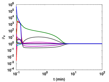
(a) Closed system

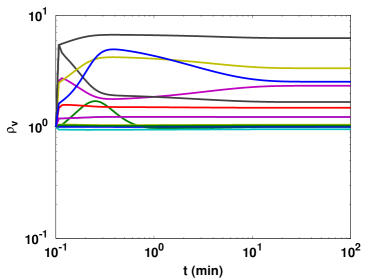
(b) Open system

Figure 6: Simulation: equilibria. For each reaction, the ratio ${\tilde{V}}_{0}=K^{v}\circ X^{v}$ (31) of the forward to backward reaction flows, is plotted. (a) Closed system: each ratio tends to unity: the steady state is a thermodynamic equilibrium. (b) Open system: some ratios tend to a non-unity value: the steady state is a not a thermodynamic equilibrium.

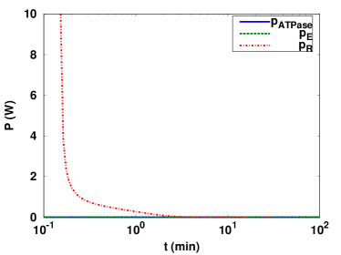
(a) Closed system

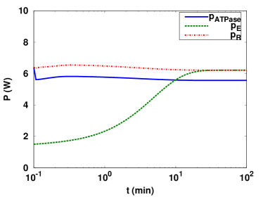
(b) Open system

Figure 7: Simulation: energy flows. Three energy flows are plotted: $P_{E}$ the external energy flow, $P_{R}$ the energy dissipated in all reactions (including $ATPase$), $P_{ATPase}$ the power consumed by the processes represented by the $ATPase$ reaction. (a) There is no external energy flow or $ATPase$ reaction flow: $P_{R}$ tends to zero as the energy in the internal species is used up. (b) There is external energy flow and $ATPase$ reaction flow: $P_{R}$ tends to $P_{E}$ as the energy in the internal species is used up. In this case, at steady-state about 90% of the energy is associated with processes represented by the $ATPase$ reaction.

The bond graph model of Figure 5 with reaction kinetics defined by Equation (53) was compiled into ordinary differential equations using the bond graph software MTT (model transformation tools) [49]. Free energy constants were obtained using the methods of § 3.1 and the kinetic parameters were derived as in § 3.2. The reduced order equations (64) § A.1 were simulated using the lsode solver within GNU Octave [50] numerical software with a maximum time step of 0.01min for two cases:

Closed system.

The flows associated with $ATPase$ and $Fout$ were constrained to be zero. Initial conditions were defined in Lambeth and Kushmerick [23, Table 3], together with the extra equations from page 813 describing the redox potential (~R) and total creatine abundance, respectively:

$$\frac{X_{NAD}}{X_{NADH}} =1000 X_{Cr}+X_{PCr} =40\text{mM}$$ (62)

The base units used by Lambeth and Kushmerick [23] are mM for concentration and minutes for time. These units have been used in the following figures except that flows are converted to M/s and concentrations to M for computing the energy flows in Figure 7.

Figure 6(a) indicates that this steady-state is an equilibrium, providing a useful “thermodynamic validation” of the model as discussed by Lambeth and Kushmerick [23]. Figure 7(a) shows energy flows, respectively, which become zero after an initial transient as the systems settles into equilibrium.

Open system.

The flows associated with $ATPase$ and $Fout$ were enabled, and the concentration of $LACo$ was fixed at a constant small value by adding an appropriate external flow $v_{E}$. The $ATPase$ coefficient was chosen to be 0.75 corresponding to the “Moderate exercise” column of Lambeth and Kushmerick [23, Table 4]. The final equilibrium state of the closed system simulation was used as the initial state. In contrast to Figure 6(a), Figure 6(b) indicates that the steady-state of the open system is not an equilibrium as the ratio ${\tilde{V}}_{0}$ is not unity. Figure 7(b) shows energy flows which settle to non-zero values. In particular, the dissipated power (including $ATPase$) $p_{R}$ becomes equal to the external energy flow $P_{E}$. Energy flows associated with $ATPase$ are indicated separately showing that about 90% of the energy is associated with processes represented by the $ATPase$ reaction. The remainder is dissipated as heat in the other reactions.

Further figures appear in the Supplementary material.

5 Conclusion

This paper extends the bond graph approach of Gawthrop and Crampin [4] to allow the hierarchical modelling of biochemical systems with reusable subsystems and robust thermodynamic compliance. This requires two extensions: the modelling of open thermodynamical systems using energy ports and the conversion of standard enzymatic rate parameters to the parameters required by the bond graph.

The reimplimentation of “A Computational Model for Glycogenolysis in Skeletal Muscle”, originally presented by Lambeth and Kushmerick [23], in a bond graph formulation verifies the utility of the bond graph approach. In particular, the discipline imposed by the bond graph reformulation focuses on four potential problems with the original model: lack of robustness caused by the separate specification of the identical equilibrium constant for two parallel reactions ($GPa$ & $GPb$); stoichiometric inconsistency arising from equating two versions of the glycogen molecule; the use of an irreversible reaction ($ATPase$); and confusion arising from reaction directionality ($TPI$). A further advantage of bond graph modelling illustrated by this example is the automatic generation of stoichiometric matrices and hence conserved moieties. Currently, these must be identified and imposed by model developers and this becomes a laborious process with increasing system sizes.

The model of enzymatic reactions used in this paper is that previously derived by Gawthrop and Crampin [4]. The relationship between this particular bond graph formulation and some models of enzyme kinetics developed by Liebermeister et al. [11] is explored in the paper. Future work will examine the development of bond graph representations for a wider range of enzyme models [51]. This would facilitate the inclusion of allosteric modulation, such as that exerted by AMP over the $GPb$ reaction.

Metabolic control analysis (MCA) [52] analyses the feedback control behaviour via sensitivity. There is a well-established theory of sensitivity bond graphs [53, 54, 55], which we will use to give a bond graph interpretation of MCA. A number of authors have discussed the role of control theory in systems biology [56, 57, 58, 59, 60] and there is a well-established theory of control in the context of bond graphs [61, 62, 63]. Future work will examine feedback control of biochemical networks from the bond graph point of view. Metabolic networks are further controlled over longer time scales by gene expression modulation of maximum reaction rate. Thus, future work will also examine the modulation of energy flows by gene expression as, for example, found in the Warburg effect [64].

An important feature of bond graphs not utilised in this paper is the ability to interconnect different physical domains. Future work will examine chemo-electrical and chemo-mechanical transduction as, for example, found in the cardiac myocyte.

Data accessibility

A virtual reference environment [43] is available for this paper at https://sourceforge.net/projects/hbgm/. The simulation parameters are listed in the Supplementary material.

Competing interests

The authors have no competing interests.

Authors’ contribution

ons] All authors contributed to drafting and revising the paper, and they affirm that they have approved the final version of the manuscript.

Acknowledgements

Peter Gawthrop would like to thank the Melbourne School of Engineering for its support via a Professorial Fellowship. The authors would like to thank Dr. Ivo Siekmann for alerting them to, and discussing the contents of, reference [39] and Dr Daniel Hurley for creating the virtual reference environment [43] for this paper. The authors would like to thank the referees for their encouraging and insightful comments which lead to an improved manuscript.

Funding statement

This research was in part conducted and funded by the Australian Research Council Centre of Excellence in Convergent Bio-Nano Science and Technology (project number CE140100036), and by the Virtual Physiological Rat Centre for the Study of Physiology and Genomics, funded through NIH grant P50-GM094503.

Appendix A Supplementary Material

A.1 Reduced-order equations

This section includes material from Gawthrop and Crampin [4, §3(c)] about using reduced-order equations for simulation.

Given the reaction flows $V$ of Equation (17), the rate of change of the internal states is given by:

$$\dot{X}_{i}=N_{i}V$$ (63)

As discussed by number of authors the presence of conserved moieties leads to potential numerical difficulties with the solution of Equation (63) [65, 66]. Using the notation of Gawthrop and Crampin [4, §3(c)], the reduced-order state $x$ and the internal state $X_{i}$ are given by:

$$\dot{x} =L_{xX}N_{i}V X_{i}=L_{Xx}x+G_{X}X_{i}(0)$$ (64)

Equation (64) was used to generate all of the simulation figures in this paper.

A.2 Conversion of kinetic data

Reaction	$K^{eq}$	$V_{maxf}$	$V_{maxr}$	$K^{M}_{a}$	$K^{M}_{b}$
ADK	2.210e+00	8.800e-01	–	8.640e-02	1.225e-01
CK	2.330e+02	5.000e-01	–	1.330e+01	1.499e-01
ALD	9.500e-05	1.040e-01	–	5.000e-02	2.000e+00
TPI	1.923e+01	1.200e+01	–	3.200e-01	6.100e-01
ENO	4.900e-01	1.920e-01	–	1.000e-01	3.700e-01
Fout	1.000e+00	2.000e+02	–	1.000e+06	1.000e+06
PGM	1.800e-01	1.120e+00	–	2.000e-01	1.400e-02
GAPDH	8.900e-02	1.265e+00	–	6.525e-05	2.640e-06
LDH	1.620e+04	1.920e+00	–	6.700e-04	1.443e+01
PGK	5.711e+04	1.120e+00	–	1.600e-05	4.200e-01
PK	1.030e+04	1.440e+00	–	2.400e-02	7.966e+00
GPa	4.200e-01	2.000e-02	–	4.000e+00	2.700e+00
GPb	4.200e-01	3.000e-02	–	2.000e-01	1.500e+00
PGI	4.500e-01	–	8.800e-01	4.800e-01	1.190e-01
PGLM	1.662e+01	4.800e-01	–	6.300e-02	3.000e-02
PFK	2.420e+02	5.600e-02	–	1.440e-02	1.085e+01
ATPase	2.497e+05	7.500e+02	–	1.000e+06	1.000e+12

Table 2: Parameters from Lambeth and Kushmerick [23, Tables 1&2].

Species	K	$\frac{\mu_{0}}{RT}$
ADP	7.677e-01	-2.643e-01
AMP	2.776e-03	-5.887e+00
ATP	4.692e+02	6.151e+00
Cr	6.174e-01	-4.822e-01
P	2.447e-03	-6.013e+00
PCr	1.620e+00	4.822e-01
DHAP	1.038e+00	3.718e-02
FBP	1.968e-03	-6.231e+00
GAP	1.996e+01	2.994e+00
DPG	1.512e+06	1.423e+01
LAC	1.748e-18	-4.089e+01
LACo	1.748e-18	-4.089e+01
NAD	1.659e+03	7.414e+00
NADH	6.026e-04	-7.414e+00
P2G	2.406e-01	-1.425e+00
P3G	4.330e-02	-3.140e+00
PEP	4.910e-01	-7.114e-01
PYR	7.795e-08	-1.637e+01
F6P	7.792e-04	-7.157e+00
G1P	5.827e-03	-5.145e+00
G6P	3.506e-04	-7.956e+00
GLY	1.000e+00	0.000e+00

Table 3: Bond graph species parameters used in simulation (See § 3.1

Reaction	$v_{max}$	$k_{v}$	$\rho_{v}$
ADK	3.439e+02	4.398e-02	6.092e-01
CK	2.418e-02	1.863e-01	1.000e+00
ALD	1.040e+02	9.840e-05	2.375e-06
TPI	1.082e+03	5.760e-01	9.098e-01
ENO	1.695e+02	2.124e-02	1.169e-01
Fout	1.000e+05	8.738e-13	5.000e-01
PGM	3.136e+02	2.425e-03	7.200e-01
GAPDH	3.953e+02	1.653e-03	6.875e-01
LDH	1.096e+03	1.796e-14	4.292e-01
PGK	3.527e+02	5.847e+00	6.851e-01
PK	4.494e+01	2.823e-04	9.688e-01
GPa	1.233e+01	6.035e-03	3.836e-01
GPb	2.841e+01	4.635e-04	5.303e-02
PGI	5.674e+02	5.978e-05	6.448e-01
PGLM	1.337e+01	1.023e-05	9.721e-01
PFK	4.239e+01	3.985e-03	2.430e-01
ATPase	6.001e+05	3.755e+08	1.998e-01

Table 4: Bond graph reaction parameters used in simulation (See § 3.2

Using the methods of § 3.1, the equilibrium constants quoted by Lambeth and Kushmerick [23, Tables 1&2] (Table 2) were converted into the free-energy constants required by the bond graph formulation and are listed in Table 3.

Using the methods of § 3.2, the reaction constants quoted by Lambeth and Kushmerick [23] (Table 2) were converted into the reaction constants required by the bond graph formulation of § 3.2 and are listed in Table 4.

Section A.3 looks at mass-action reactions as used for $ATPase$, § A.4 looks at the relationship of the approach in § 3.2 to the direct-binding modular rate law of Liebermeister et al. [11], § A.5 to the common modular rate law of Liebermeister et al. [11] and § A.6 to the computational model of Lambeth and Kushmerick [23].

A.3 Mass-action reactions

The mass-action formulation of chemical equations reveals key issues encountered in converting kinetic data from enzymatic models into the form required by a bond graph model. Enzyme catalysed reactions are discussed in § 3.2.

The mass-action formulation presented by Gawthrop and Crampin [4, Equation 2.6] uses the Marcelin formulation rewritten here as:

$$v =\kappa\left(V_{0}^{+}-V_{0}^{-}\right) \text{where }V_{0}^{+} =e^{A^{f}/RT} \text{and }V_{0}^{-} =e^{A^{r}/RT}$$ (65)

In terms of the reaction $A{\;\xrightleftharpoons{}\;}B$

$$V_{0}^{+} =K_{a}x_{a} V_{0}^{-} =K_{b}x_{b}$$ (66)

In terms of the reaction $A+B{\;\xrightleftharpoons{}\;}2C$

$$V_{0}^{+} =K_{a}x_{a}K_{b}x_{b} V_{0}^{-} =\left(K_{c}x_{c}\right)^{2}$$ (67)

One standard way of writing the Mass-action rate of $A{\;\xrightleftharpoons{}\;}B$

$$v =\kappa_{eq}\left(x_{a}-\frac{1}{K_{eq}}x_{b}\right) \text{where }K_{eq} =\frac{K_{a}}{K_{b}}$$ (68)

similarly, $A+B{\;\xrightleftharpoons{}\;}2C$ can be rewritten as

$$v =\kappa_{eq}\left(x_{a}x_{b}-\frac{1}{K_{eq}}x_{c}^{2}\right) \text{where }K_{eq} =\frac{K_{a}K_{b}}{K_{c}^{2}}$$ (69)

Define $K^{f}$ as the constant on the substrate side and $K^{r}$ as the constant on the product side. In the case of $A{\;\xrightleftharpoons{}\;}B$

$$K^{f} =K_{a} \text{and }K^{r} =K_{b}$$ (70)

and in the case of $A+B{\;\xrightleftharpoons{}\;}2C$

$$K^{f} =K_{a}K_{b} \text{and }K^{r} =K_{c}^{2}$$ (71)

It follows that:

$$\kappa_{eq} =K^{f}\kappa \text{and }K_{eq} =\frac{K^{f}}{K_{r}}$$ (72)

As $K_{f}$ can be computed from $K$, which in turn can be deduced as discussed in § 3.1, it follows that $\kappa$ can be deduced from $\kappa_{eq}$.

A.4 Relation to the Direct Binding Modular Rate Law of Liebermeister et al. [11]

It is now shown using an example that Equation (53) is of the same form as the direct binding modular rate law of Liebermeister et al. [11]. Consider the enzyme catalysed reaction $A+B{\;\xrightleftharpoons{}\;}2C$ In this case:

$$V_{0}^{+}=K_{a}K_{b}x_{a}x_{b},\;V_{0}^{-}=K_{c}^{2}x_{c}^{2}$$ (73)

Equation (53) is of the form:

$$v=\frac{v_{max}^{+}\frac{K_{a}K_{b}x_{a}x_{b}}{K_{v}^{+}}-v_{max}^{-}\frac{K_{c}^{2}x_{c}^{2}}{K_{v}^{-}}}{1+\frac{K_{a}K_{b}x_{a}x_{b}}{K_{v}^{+}}+\frac{K_{c}^{2}x_{c}^{2}}{K_{v}^{-}}}$$ (74)

The direct binding modular rate law is given by Equation (4) of Liebermeister et al. [11] and in the notation of this paper is:

$$v=u\frac{k^{+}\frac{x_{a}}{K^{M}_{a}}\frac{x_{b}}{K^{M}_{b}}-k^{-}\left(\frac{x_{c}}{K^{M}_{c}}\right)^{2}}{1+\frac{x_{a}}{K^{M}_{a}}\frac{x_{b}}{K^{M}_{b}}+\left(\frac{x_{c}}{K^{M}_{c}}\right)^{2}}$$ (75)

Equations (74) and (75) are identical if we set:

$$v_{max}^{+} =uk^{+} v_{max}^{-} =uk^{-} K_{v}^{+} =\frac{K^{M}_{a}K^{M}_{b}}{K_{a}K_{b}} K_{v}^{-} =\left(\frac{K^{M}_{c}}{K_{c}}\right)^{2}$$ (76)

A.5 Relation to the Common Modular Rate Law of Liebermeister et al. [11]

However, Equation (53) is not the same as the common modular rate law of Liebermeister et al. [11]. In the context of the reaction $A+B{\;\xrightleftharpoons{}\;}2C$, the common modular rate law of Liebermeister et al. [11] is of the form:

$$v=u\frac{k^{+}\frac{x_{a}}{K^{M}_{a}}\frac{x_{b}}{K^{M}_{b}}-k^{-}\left(\frac{x_{c}}{K^{M}_{c}}\right)^{2}}{1+\frac{x_{a}}{K^{M}_{a}}+\frac{x_{b}}{K^{M}_{b}}+\frac{x_{a}}{K^{M}_{a}}\frac{x_{b}}{K^{M}_{b}}+2\frac{x_{c}}{K^{M}_{c}}+\left(\frac{x_{c}}{K^{M}_{c}}\right)^{2}}$$ (77)

As discussed by Liebermeister et al. [11], the additional denominator terms imply that Equation (77) is not the same as Equation (75) but can be considered an approximation to it. However, in the case of reaction $A{\;\xrightleftharpoons{}\;}B$, the common modular and direct binding modular reaction rates are identical.

A.6 Relation to the computational model of Lambeth and Kushmerick [23]

The general enzyme catalysed reaction between two species is given by $A{\;\xrightleftharpoons{}\;}B$ and the corresponding rate is written by Lambeth and Kushmerick [23] as:

$$v=\frac{V_{maxf}\frac{x_{a}}{K^{M}_{a}}-V_{maxr}\frac{x_{b}}{K^{M}_{b}}}{1+\frac{x_{a}}{K^{M}_{a}}+\frac{x_{b}}{K^{M}_{b}}}\text{ where }V_{maxr}=V_{maxf}\frac{K^{M}_{b}K^{M}_{eq}}{K^{M}_{a}}$$ (78)

In this case $V_{0}^{+}=K_{a}X_{a}$ and $V_{0}^{-}=K_{b}X_{b}$ hence Equation (53) becomes:

$$v=\frac{v_{max}}{k_{v}}\frac{K_{a}X_{a}-K_{b}X_{b}}{1+\left(\left(1-\rho_{v}\right)\frac{K_{a}}{k_{v}}X_{a}+\rho_{v}\frac{K_{b}}{k_{v}}X_{b}\right)}$$ (79)

Comparing Equations (78) and (79) and using Equation (54) it follows that they are identical if:

$$K^{M}_{a}=\frac{1}{1-\rho_{v}}\frac{k_{v}}{K_{a}}\text{ and }K^{M}_{b}=\frac{1}{\rho_{v}}\frac{k_{v}}{K_{b}}$$ (80)

or:

$$k_{v}=(1-\rho_{v})K_{a}K^{M}_{a}\text{ and }k_{v}=\rho_{v}K_{b}K^{M}_{b}$$ (81)

Having deduced $\rho_{v}$ from the given data using Equation (54), $k_{v}$ can then be deduced from $K^{M}_{a}$ using $K_{a}$, as shown in § 3.1.

Alternatively comparing Equation (52) with Equation (78) gives:

$$k_{v}^{+}=\frac{K^{M}_{a}}{K_{a}}\text{ and }k_{v}^{-}=\frac{K^{M}_{b}}{K_{b}}$$ (82)

Using the expressions for $k_{v}^{+}$ and $k_{v}^{-}$ (52) gives the same result.

A.7 TPI

The equilibrium constant is given as $K_{eq}=0.052$. However this gives the wrong value of $K_{eqcombo}$. Because the reaction is specified in the “wrong” direction, it is assumed that $K_{eq}$ should be the reciprocal of the given value, ie $K_{eq}=19.23$. Beard [41] quotes $K_{eq}=19.87$; so this alteration seems to be correct.

A.8 Hierarchical modelling

The bond graphs of the subsystems GAP2LAC and CrAMP appear in Figures 8 and 9.

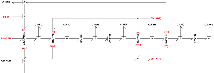
Figure 8: Submodel: GAP2LAC

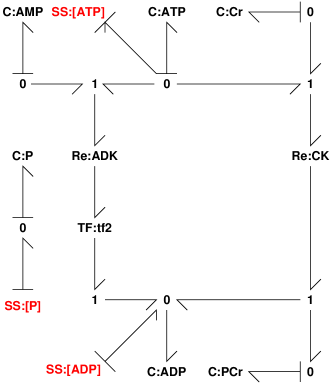
Figure 9: Submodel: CrAMP

The ODEs, and corresponding flows, automatically generated from the Bond Graph are given by the following equations

$$\dot{X}_{adp} ={2V_{adk}-V_{pgk}-V_{pk}+V_{pfk}+V_{atpase}+V_{ck}}$$ (83)

$$\dot{X}_{amp} ={-V_{adk}}$$

$$\dot{X}_{atp} ={-V_{adk}+V_{pgk}+V_{pk}-V_{pfk}-V_{atpase}-V_{ck}}$$

$$\dot{X}_{cr} ={-V_{ck}}$$

$$\dot{X}_{p} ={-V_{gpa}-V_{gpb}+V_{atpase}-V_{gapdh}}$$

$$\dot{X}_{pcr} ={V_{ck}}$$

$$\dot{X}_{dhap} ={V_{ald}+V_{tpi}}$$

$$\dot{X}_{fbp} ={V_{pfk}-V_{ald}}$$

$$\dot{X}_{gap} ={V_{ald}-V_{tpi}-V_{gapdh}}$$

$$\dot{X}_{dpg} ={-V_{pgk}+V_{gapdh}}$$

$$\dot{X}_{lac} ={-V_{fout}+V_{ldh}}$$

$$\dot{X}_{laco} ={V_{fout}}$$

$$\dot{X}_{nad} ={-V_{gapdh}+V_{ldh}}$$

$$\dot{X}_{nadh} ={V_{gapdh}-V_{ldh}}$$

$$\dot{X}_{p2g} ={-V_{eno}+V_{pgm}}$$

$$\dot{X}_{p3g} ={V_{pgk}-V_{pgm}}$$

$$\dot{X}_{pep} ={-V_{pk}+V_{eno}}$$

$$\dot{X}_{pyr} ={V_{pk}-V_{ldh}}$$

$$\dot{X}_{f6p} ={V_{pgi}-V_{pfk}}$$

$$\dot{X}_{g1p} ={V_{gpa}+V_{gpb}-V_{pglm}}$$

$$\dot{X}_{g6p} ={-V_{pgi}+V_{pglm}}$$

$$\dot{X}_{gly} ={0}$$

$$V_{adk} ={{\left(v_{adk}{\left(-k_{adp}^{2}X_{adp}^{2}+k_{amp}k_{atp}X_{amp}X_{atp}\right)}\right)}\over{\left(k_{adk}+k_{adp}^{2}X_{adp}^{2}\rho_{adk}-k_{amp}k_{atp}X_{amp}X_{atp}\rho_{adk}+k_{amp}k_{atp}X_{amp}X_{atp}\right)}}$$ (84)

$$V_{ck} ={{\left(v_{ck}{\left(-k_{adp}k_{pcr}X_{adp}X_{pcr}+k_{atp}k_{cr}X_{atp}X_{cr}\right)}\right)}\over{\left(k_{adp}k_{pcr}X_{adp}X_{pcr}\rho_{ck}-k_{atp}k_{cr}X_{atp}X_{cr}\rho_{ck}+k_{atp}k_{cr}X_{atp}X_{cr}+k_{ck}\right)}}$$

$$V_{ald} ={{\left(v_{ald}{\left(-k_{dhap}k_{gap}X_{dhap}X_{gap}+k_{fbp}X_{fbp}\right)}\right)}\over{\left(k_{ald}+k_{dhap}k_{gap}X_{dhap}X_{gap}\rho_{ald}-k_{fbp}X_{fbp}\rho_{ald}+k_{fbp}X_{fbp}\right)}}$$

$$V_{tpi} ={{\left(v_{t\pi}{\left(-k_{dhap}X_{dhap}+k_{gap}X_{gap}\right)}\right)}\over{\left(k_{dhap}X_{dhap}\rho_{t\pi}-k_{gap}X_{gap}\rho_{t\pi}+k_{gap}X_{gap}+k_{t\pi}\right)}}$$

$$V_{eno} ={{\left(v_{eno}{\left(k_{p2g}X_{p2g}-k_{pep}X_{pep}\right)}\right)}\over{\left(k_{eno}-k_{p2g}X_{p2g}\rho_{eno}+k_{p2g}X_{p2g}+k_{pep}X_{pep}\rho_{eno}\right)}}$$

$$V_{fout} ={{\left(v_{fout}{\left(k_{lac}X_{lac}-k_{laco}X_{laco}\right)}\right)}\over{\left(k_{fout}-k_{lac}X_{lac}\rho_{fout}+k_{lac}X_{lac}+k_{laco}X_{laco}\rho_{fout}\right)}}$$

$$V_{pgm} ={{\left(v_{pgm}{\left(-k_{p2g}X_{p2g}+k_{p3g}X_{p3g}\right)}\right)}\over{\left(k_{p2g}X_{p2g}\rho_{pgm}-k_{p3g}X_{p3g}\rho_{pgm}+k_{p3g}X_{p3g}+k_{pgm}\right)}}$$

$$V_{gapdh} ={{\left(v_{gapdh}{\left(-k_{dpg}k_{nadh}X_{dpg}X_{nadh}+k_{gap}k_{nad}k_{p}X_{nad}X_{p}X_{gap}\right)}\right)}\over{\left(k_{dpg}k_{nadh}X_{dpg}X_{nadh}\rho_{gapdh}-k_{gap}k_{nad}k_{p}X_{nad}X_{p}X_{gap}\rho_{gapdh}+k_{gap}k_{nad}k_{p}X_{nad}X_{p}X_{gap}+k_{gapdh}\right)}}$$

$$V_{ldh} ={{\left(v_{ldh}{\left(-k_{lac}k_{nad}X_{lac}X_{nad}+k_{nadh}k_{pyr}X_{nadh}X_{pyr}\right)}\right)}\over{\left(k_{lac}k_{nad}X_{lac}X_{nad}\rho_{ldh}+k_{ldh}-k_{nadh}k_{pyr}X_{nadh}X_{pyr}\rho_{ldh}+k_{nadh}k_{pyr}X_{nadh}X_{pyr}\right)}}$$

$$V_{pgk} ={{\left(v_{pgk}{\left(-k_{adp}k_{dpg}X_{adp}X_{dpg}+k_{atp}k_{p3g}X_{p3g}X_{atp}\right)}\right)}\over{\left(k_{adp}k_{dpg}X_{adp}X_{dpg}\rho_{pgk}-k_{adp}k_{dpg}X_{adp}X_{dpg}-k_{atp}k_{p3g}X_{p3g}X_{atp}\rho_{pgk}-k_{pgk}\right)}}$$

$$V_{pk} ={{\left(v_{pk}{\left(-k_{adp}k_{pep}X_{adp}X_{pep}+k_{atp}k_{pyr}X_{pyr}X_{atp}\right)}\right)}\over{\left(k_{adp}k_{pep}X_{adp}X_{pep}\rho_{pk}-k_{adp}k_{pep}X_{adp}X_{pep}-k_{atp}k_{pyr}X_{pyr}X_{atp}\rho_{pk}-k_{pk}\right)}}$$

$$V_{gpa} ={{\left(k_{gly}X_{gly}v_{gpa}{\left(-k_{g1p}X_{g1p}+k_{p}X_{p}\right)}\right)}\over{\left(k_{g1p}k_{gly}X_{g1p}X_{gly}\rho_{gpa}-k_{gly}k_{p}X_{gly}X_{p}\rho_{gpa}+k_{gly}k_{p}X_{gly}X_{p}+k_{gpa}\right)}}$$

$$V_{gpb} ={{\left(k_{gly}X_{gly}v_{gpb}{\left(-k_{g1p}X_{g1p}+k_{p}X_{p}\right)}\right)}\over{\left(k_{g1p}k_{gly}X_{g1p}X_{gly}\rho_{gpb}-k_{gly}k_{p}X_{gly}X_{p}\rho_{gpb}+k_{gly}k_{p}X_{gly}X_{p}+k_{gpb}\right)}}$$

$$V_{pgi} ={{\left(v_{pgi}{\left(-k_{f6p}X_{f6p}+k_{g6p}X_{g6p}\right)}\right)}\over{\left(k_{f6p}X_{f6p}\rho_{pgi}-k_{g6p}X_{g6p}\rho_{pgi}+k_{g6p}X_{g6p}+k_{pgi}\right)}}$$

$$V_{pglm} ={{\left(v_{pglm}{\left(-k_{g1p}X_{g1p}+k_{g6p}X_{g6p}\right)}\right)}\over{\left(k_{g1p}X_{g1p}\rho_{pglm}-k_{g1p}X_{g1p}-k_{g6p}X_{g6p}\rho_{pglm}-k_{pglm}\right)}}$$

$$V_{pfk} ={{\left(v_{pfk}{\left(-k_{adp}k_{fbp}X_{adp}X_{fbp}+k_{atp}k_{f6p}X_{f6p}X_{atp}\right)}\right)}\over{\left(k_{adp}k_{fbp}X_{adp}X_{fbp}\rho_{pfk}-k_{atp}k_{f6p}X_{f6p}X_{atp}\rho_{pfk}+k_{atp}k_{f6p}X_{f6p}X_{atp}+k_{pfk}\right)}}$$

$$V_{atpase} ={{\left(v_{atpase}{\left(-k_{adp}k_{p}X_{adp}X_{p}+k_{atp}X_{atp}\right)}\right)}\over{\left(k_{adp}k_{p}X_{adp}X_{p}\rho_{atpase}-k_{atp}X_{atp}\rho_{atpase}+k_{atp}X_{atp}+k_{atpase}\right)}}$$

A.9 Simulation

Further figures corresponding to Section 4.3 appear in Figures 10, 11 and 12.

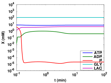
(a) Closed system

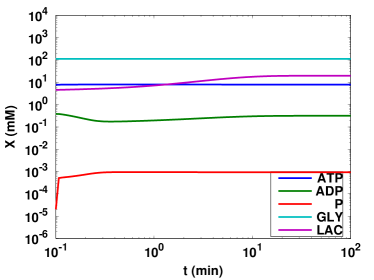
(b) Open system

Figure 10: Simulated concentrations. Evolution of the concentrations for $ATP$, $ADP$, $P$, $GLY$ and $LAC$ corresponds to the situation in Lambeth and Kushmerick [23, Figure 2] except that they use unit initial states. Following an initial transient, the species concentrations reach steady-state values for both the closed and open systems (cf Figure 2).

(a) Closed system

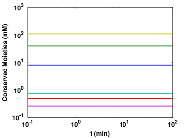
(b) Open system

Figure 11: Conserved Moieties. The sum of each conserved moiety remains constant.

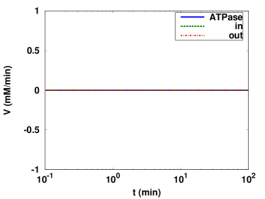
(a) Closed system

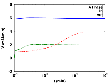
(b) Open system

Figure 12: Simulated mass flows. Both plots show the input mass flow (though SS:GLYo), the output mass flow (though Re:Fout) and the ATP flux (though Re:ATPase) (a) In the closed system, the flows are zero. (b) In the open system, the three flows reach a constant steady state. The final value of ATP flow is 5.9mM/min; this is close to to value of 6.1mM/min quoted in the “Moderate exercise” column of Lambeth and Kushmerick [23, Table 4]

Closed system.

Figure 11(a) provides another validity check, showing that the conserved moieties are constant; because the reduced order equations (§ A.1) were used, this constraint is automatically enforced and thus numerical drift is avoided. Figure 12(a) shows mass flows within the system.

Open system.

Figure 10(b) shows the evolution of simulated concentrations for $ATP$, $ADP$, $P$, $GLY$ and $LAC$ which reach new steady state values due to flows induced by the $ATPase$ reaction. As with Figure 11(a), Figure 11(b) shows the conserved moieties are constant for the open system. In contrast to Figure 12(a), Figure 12(b) shows mass flow which, in this open-system context settle to non-zero values.

A.10 Virtual Reference Environment

The software required to generate all of the simulation figures shown in this paper from the bond graph representation is packaged in the form of a Virtual Reference Environment [43]. It is available at https://sourceforge.net/projects/hbgm/.

References

- Karr et al. [2012] Jonathan R. Karr, Jayodita C. Sanghvi, Derek N. Macklin et al. A whole-cell computational model predicts phenotype from genotype. Cell, 150(2):389 – 401, 2012.
- Kohl and Noble [2009] Peter Kohl and Denis Noble. Systems biology and the virtual physiological human. Mol Syst Biol, 5, July 2009.
- Hunter et al. [2013] Peter Hunter, Tara Chapman, Peter V. Coveney et al. A vision and strategy for the virtual physiological human: 2012 update. Interface Focus, 3(2), 2013.
- Gawthrop and Crampin [2014] Peter J. Gawthrop and Edmund J. Crampin. Energy-based analysis of biochemical cycles using bond graphs. Proceedings of the Royal Society A: Mathematical, Physical and Engineering Science, 470(2171), 2014.
- Hill [1989] Terrell L Hill. Free energy transduction and biochemical cycle kinetics. Springer-Verlag, New York, 1989.
- Beard and Qian [2010] Daniel A Beard and Hong Qian. Chemical biophysics: quantitative analysis of cellular systems. Cambridge University Press, 2010.
- Keener and Sneyd [2009] James P Keener and James Sneyd. Mathematical Physiology: I: Cellular Physiology, volume 1. Springer, 2nd edition, 2009.
- Atkins and de Paula [2011] Peter Atkins and Julio de Paula. Physical Chemistry for the Life Sciences. Oxford University Press, 2nd edition, 2011.
- Henry et al. [2007] Christopher S. Henry, Linda J. Broadbelt, and Vassily Hatzimanikatis. Thermodynamics-based metabolic flux analysis. Biophysical Journal, 92(5):1792 – 1805, 2007.
- Ederer and Gilles [2007] Michael Ederer and Ernst Dieter Gilles. Thermodynamically feasible kinetic models of reaction networks. Biophysical Journal, 92(6):1846 – 1857, 2007.
- Liebermeister et al. [2010] Wolfram Liebermeister, Jannis Uhlendorf, and Edda Klipp. Modular rate laws for enzymatic reactions: thermodynamics, elasticities and implementation. Bioinformatics, 26(12):1528–1534, 2010.
- Gawthrop and Smith [1996] P. J. Gawthrop and L. P. S. Smith. Metamodelling: Bond Graphs and Dynamic Systems. Prentice Hall, Hemel Hempstead, Herts, England., 1996.
- Borutzky [2011] Wolfgang Borutzky. Bond Graph Modelling of Engineering Systems: Theory, Applications and Software Support. Springer, 2011.
- Karnopp et al. [2012] Dean C Karnopp, Donald L Margolis, and Ronald C Rosenberg. System Dynamics: Modeling, Simulation, and Control of Mechatronic Systems. John Wiley & Sons, 5th edition, 2012.
- Gawthrop and Bevan [2007] Peter J Gawthrop and Geraint P Bevan. Bond-graph modeling: A tutorial introduction for control engineers. IEEE Control Systems Magazine, 27(2):24–45, April 2007.
- Oster et al. [1971] George Oster, Alan Perelson, and Aharon Katchalsky. Network thermodynamics. Nature, 234:393–399, December 1971.
- Oster et al. [1973] George F. Oster, Alan S. Perelson, and Aharon Katchalsky. Network thermodynamics: dynamic modelling of biophysical systems. Quarterly Reviews of Biophysics, 6(01):1–134, 1973.
- Cellier [1991] F. E. Cellier. Continuous system modelling. Springer-Verlag, 1991.
- Greifeneder and Cellier [2012] J. Greifeneder and F.E. Cellier. Modeling chemical reactions using bond graphs. In Proceedings ICBGM12, 10th SCS Intl. Conf. on Bond Graph Modeling and Simulation, pages 110–121, Genoa, Italy, 2012.
- Thoma and Atlan [1985] Jean Thoma and Henri Atlan. Osmosis and hydraulics by network thermodynamics and bond graphs. Journal of the Franklin Institute, 319(1-2):217 – 226, 1985.
- LeFèvre et al. [1999] Jacques LeFèvre, Laurent LeFèvre, and Bernadette Couteiro. A bond graph model of chemo-mechanical transduction in the mammalian left ventricle. Simulation Practice and Theory, 7(5-6):531–552, 1999.
- Diaz-Zuccarini and Pichardo-Almarza [2011] Vanessa Diaz-Zuccarini and Cesar Pichardo-Almarza. On the formalization of multi-scale and multi-science processes for integrative biology. Interface Focus, 1(3):426–437, 2011.