Cosmological constraints from Subaru weak lensing cluster counts

Abstract

We present results of weak lensing cluster counts obtained from 11 degree² Subaru/SuprimeCam data. Although the area is much smaller than previous work dealing with weak lensing peak statistics, the number density of galaxies usable for weak lensing analysis is about twice as large as those. The higher galaxy number density reduces the noise in the weak lensing mass maps, and thus increases the signal-to-noise ratio ($S/N$) of peaks of the lensing signal due to massive clusters. This enables us to construct a weak lensing selected cluster sample by adopting a high threshold $S/N$, such that the contamination rate due to false signals is small. We find 6 peaks with $S/N>5$. For all the peaks, previously identified clusters of galaxies are matched within a separation of 1 arcmin, demonstrating good correspondence between the peaks and clusters of galaxies. We evaluate the statistical error in the weak lensing cluster counts using mock weak lensing data generated from full-sky ray-tracing simulations, and find $N_{\rm peak}=6\pm 3.1$ in an effective area of 9.0 degree². We compare the measured weak lensing cluster counts with the theoretical model prediction based on halo models and place the constraint on $\Omega_{m}-\sigma_{8}$ plane which is found to be consistent with currently standard $\Lambda$CDM models. It is demonstrated that the weak lensing cluster counts can place a unique constraint on $\sigma_{8}-c_{0}$ plane, where $c_{0}$ is the normalization of the dark matter halo mass–concentration relationship. Finally we discuss prospects for ongoing/future wide field optical galaxy surveys.

1 Introduction

The $\Lambda$-flat universe with cold dark matter ($\Lambda$CDM) is now considered as the standard theoretical framework for cosmic structure formation. In the $\Lambda$CDM paradigm, dark matter haloes of a galaxy and a cluster of galaxies form though the hierarchical bottom-up assembly of smaller structures. The averaged density profile of the dark matter haloes found in $N$-body simulations has a universal broken power-law form (Navarro et al. 1997). The universal profile is characterized by a single parameter (called the concentration parameter) describing the ratio of the scale radius (where the power-law slope is approximately $-2$) to the virial radius which defines a halo’s mass. The concentration parameter is known to be related to the halo mass, a correlation which most likely arises from the mass assembly history of haloes (Bullock et al. 2001; Zhao et al. 2009; Ludlow et al. 2014; Diemer & Kravtsov 2015). Since the mass assembly history depends on the cosmological model, the mass–concentration relation does as well (Macciò et al. 2008; Kwan et al. 2013). Therefore placing constraints on both the cosmological model and the mass–concentration relation simultaneously allows us to test the $\Lambda$CDM structure formation scenario.

Clusters of galaxies serve as one of the most important tests of the cosmic structure formation model. Due to their high virial temperatures, the dissipative cooling of baryons is less effective, and thus the density profile of clusters may be well approximated by the dark matter distribution, allowing us to test the mass–concentration relation (see for a recent review Ettori et al. 2013, and references therein). Also, cluster number counts have placed useful constraint on the cosmological parameters (Vikhlinin et al. 2009; Mantz et al. 2010; Rozo et al. 2010).

It is argued in recent studies that number counts of clusters of galaxies identified in weak lensing mass maps (which we call weak lensing cluster counts) can be a powerful probe of both the cosmological model and the mass–concentration relation (Mainini & Romano 2014; Cardone et al. 2014). This can be simply understood as follows: First, the number density of massive clusters of galaxies, which appear as high peaks on the weak lensing mass maps, depends of the cosmological model (Borgani et al. 2001; Henry 2004). Second, peak heights depend on the density profile of clusters and thus on the mass–concentration relation (King & Mead 2011; Hamana et al. 2012).

Both observational techniques and theoretical models of weak lensing cluster counts have been greatly developed in the last decade. On the observational side, systematic weak lensing cluster searches have become practicable (Miyazaki et al. 2002a, 2007; Wittman et al. 2006; Gavazzi & Soucail 2007; Schirmer et al. 2007; Kubo et al. 2009; Bellagamba et al. 2011; Shan et al. 2012). Miyazaki et al. (2007) presented the first large sample of weak lensing peaks (which are plausible candidates of clusters/groups of galaxies) in $16.7$ degree² Subaru weak lensing survey data, with 100 peaks with signal-to-noise ratio exceeding $S/N>3.7$. Shan et al. (2012) reported 301 weak lensing high peaks ($S/N>3.5$) located from 64 degree² of CFHTLS-wide data, among those peaks, they confirmed 85 groups/clusters. On the theoretical side, models of the weak lensing cluster counts have been developed: Based on the pioneering work by Bartelmann et al. (2001), some improvements have been made, including the effect of the galaxy intrinsic ellipticities (Hamana et al. 2004; Fan et al. 2010), the effect of the large-scale structures (Marian et al. 2010; Maturi et al. 2010), the effect of the diversity of the dark matter distribution within clusters (Hamana et al. 2012), and an optimal choice of the filter function (Hennawi & Spergel 2005; Maturi et al. 2005). Now, the theoretical models were tested (or calibrated) against $N$-body simulations and good agreements were found (see the above references).

In fact, weak lensing peak counts have now become a practical tool for investigating cosmological models. Liu et al. (2014a) used weak lensing peak counts combined with weak lensing power spectrum measured from the CFHTLenS data to constrain cosmological parameters. They used not only high peaks but also low peaks ($-0.04<\kappa<0.12$) in order to efficiently utilize cosmological information contained in the weak lensing mass map. They found that the constraints from peak counts are comparable to those from the cosmic shear power spectrum. Liu et al. (2014b) used weak lensing peak counts within $3<S/N<6$ from $\sim 130$ degree² of the Canada-France-Hawaii Telescope Stripe82 Survey data. They demonstrated the capability to put a constraint on the mass–concentration relation together with the cosmological parameters from weak lensing peak counts.

In this paper, we examine weak lensing cluster counts obtained from 11 degree² of weak lensing mass maps generated from deep Subaru/SuprimeCam data. In contrast to previous work (Liu et al. 2014a, b), we deal only with high peaks, with $S/N>5$. Such high peaks mostly associate with a real massive cluster of galaxies, and thus we shall use the term “weak lensing cluster counts” instead of “weak lensing peak counts”. Our higher threshold enables us to make a reliable theoretical prediction of the weak lensing cluster counts utilizing models of dark matter haloes which are well calibrated with $N$-body simulations. For the first time, we use the weak lensing cluster counts to place cosmological parameters and the mass–concentration relationship. In doing this, we explore, in an experimental manner, the capability and current issues of weak lensing cluster counts for cosmological studies.

The structure of this paper is as follows. In Section 2, we summarize the Subaru/SuprimeCam data, data processing, and weak lensing shape measurement. We also examine the additive and multiplicative bias in the measured galaxy ellipticities. In section 3, we first describe construction of weak lensing mass maps. Then we examine statistical properties of peaks paying special attention to the residual systematics associated with data reduction and/or weak lensing shear measurement. In that section, we also summarize the high $S/N$ peaks and their possible counterpart clusters of galaxies searched in known cluster databases. In Section 4, the measured weak lensing cluster counts are compared with the theoretical prediction to place constraints on the cosmological parameters and the dark matter halo mass–concentration relationship. Finally, summary and discussion are given in Section 5. In Appendix A, the method for conversion of WCSs from the astrometric SIP to TPV convention, which is used in the present work, is described.

2 Data analysis

2.1 Data set and data processing

Table 1: Summary of data sets. See Fig. 4 for the coordinate and shape of each field

Field name	Areaa	$n_{g}$b	Seeingc
XMM-LSS	3.6 (2.8)	23.7 (20.9)	0.51–0.71
COSMOS	2.1 (1.6)	28.8 (26.3)	0.50–0.53
Lockman-hole	2.1 (1.6)	25.5 (23.8)	0.42–0.55
ELAIS N1	3.6 (2.9)	24.6 (22.0)	0.45–0.69

^a Area after masking regions affected by bright stars in unit of degree². The numbers in parentheses are the effective area ($A^{eff}$) after cutting the edge regions within 1.5 arcmin from the boundary.
^b The mean number density of galaxies used for the weak lensing analysis in the unit of arcmin^-2. The numbers in parentheses are the effective number density defined by $n_{g}^{eff}=(\sum_{i}w_{i})^{2}/\sum_{i}w_{i}^{2}/A^{eff}$ (Heymans et al. 2012).
^c Seeing full width at half-maximum in the unit of arcsec. The smallest and largest values among the pointings are given.

We collected $i^{\prime}$-band data taken with the Subaru/SuprimeCam (Miyazaki et al. 2002b) from the data archive SMOKA (Baba et al. 2002), under the following three conditions: data, which are composed of a number of pointings, are contiguous at least 2 degree², the exposure time for each pointing is longer than 1800 sec, and the seeing full width at half-maximum (FWHM) of each exposure is better than 0.7 arcsec. Four data sets meet these requirements and are summarized in Table 1. Data of each pointing are composed of several dithered exposures. Dithering scales are a few arcmin except for the COSMOS field for which a specific dithering pattern was adopted (a combination of dithered pointings of the normal “north is up” exposures and 90 degree rotated exposures, see Taniguchi et al. 2007).

Each CCD dataset was reduced using an image analysis pipeline, hscPipe, developed for Hyper SuprimeCam (Miyazaki et al. 2012) data (Furusawa et al. in prep.), which is based on LSST-stack (Ivezic et al. 2008; Axelrod et al. 2010), with being tuned for SuprimeCam data. The mosaic stacking was done with hscPipe using the standard correlation technique between star positions on CCD coordinates and an external star catalog (we used the SDSS DR8), and also between the star positions among different exposures. We made stacked data on a pointing-to-pointing basis except for COSMOS data for which a single stacked data was made by using SCAMP (Bertin 2006) and SWarp (Bertin et al. 2002) from all the CCD data. Object detections were performed with SExtractor (Bertin & Arnouts 1996). Stars are selected in a standard way by identifying the appropriate branch in the magnitude-object size (FWHM) plane, along with the detection significance cut $S/N>10$. The number density of stars is found to be $\sim 1$ arcmin^-2 for the four fields. We only use galaxies met the following three conditions, (i) the detection significance of $S/N>8$, (ii) FWHM is larger than the stellar branch, and (iii) the AB magnitude (for which we adopted SExtractor’s MAG_AUTO) is in the range of $22<i^{\prime}<25$. The number density of resulting galaxy catalogue varies among pointings due mainly to the variation in the seeing and weakly to the exposure time (see Fig. 1).

Figure 1: The number densities of galaxies used for weak lensing analysis are plotted against the seeing FWHM for each pointing. The different symbols represent the different exposure time.

2.2 Weak lensing shear estimate

For the weak lensing shear estimates, we employ lensfit (Miller et al. 2007; Kitching et al. 2008; Miller et al. 2013), which is a model-fitting method. We refer the reader to the above references for details of its method, implementation, and results from tests on image simulations. One important function of lensfit which should be noticed is that galaxies on each individual exposure image are fitted by models that have been convolved with the PSF for the image, and the resulting likelihoods multiply to obtain the final combined likelihood. This can avoid problematic issues in measuring weak lensing shears from a stacked image; including deformation of object shapes by interpolation of pixel data needed for resampling onto a co-added pixel grid (Rhodes et al. 2007; Hamana & Miyazaki 2008; Miller et al. 2013), and a complex PSF variation over a stacked image caused by co-addition of different individual PSFs (Hamana et al. 2013).

Application of lensfit to SuprimeCam data was first done by Dietrich et al. (2012). We used the lensfit software suite which is designed for dealing with SuprimeCam data. For the actual implementation of lensfit, we basically follow one developed for CFHTLenS (Miller et al. 2013) and thus the method is likelihood-based, and we adopt the same priors for the galaxy model. In order to adjust lensfit to SuprimeCam data, we have made following two modifications. (1) The size of postage-stamp image for galaxies was set to be $40\times 40$ ($48\times 48$ for CFHTLenS) because of the following two reasons: The first is the difference in the CCD pixel sizes between SuprimeCam (0.202 arcsec) and MegaCam on CFHT (0.185 arcsec), and second is that more smaller galaxies are detected in SuprimeCam data owing to their deeper image depth. (2) The definition of a boundary of objects was modified in the following way. In the analysis of CFHTLenS (Miller et al. 2013), $2\sigma$ isophote was adopted for a boundary of objects in the following two processes; (I) masking neighbour objects in the same postage-stamp image, and (II) clipping of possible blending objects identified by the overlapping of isophotes of close objects and by a mismatch between the peak and centroid positions. Since the noise level of an image depends on the depth of data and our data are much deeper than CFHTLenS data (thus smaller $\sigma$), adopting the same $2\sigma$ isophote extends the object boundary to outer skirt and significantly increases a chance a object to be classified as a blending object and to be rejected. We thus decided to set the threshold isophote ($f_{\rm th}\sigma$) being the CFHTLenS-2$\sigma$ corresponding value; $f_{\rm th}=2\sqrt{T_{exp}/900{\rm sec}}$, where $T_{exp}$ is the total exposure time for each pointing and $900{\rm sec}$ is the SuprimeCam corresponding exposure time of the CFHTLenS ($3600{\rm sec}$). Galaxies that are excluded in the process of lensfit shape measurement is mostly due to the above criteria, plus a small fraction of failures in the model-fitting step. The fractions of excluded galaxies vary among pointings, and the average value is 0.22. This is comparable to that for the CFHTLenS ($\sim 0.2$), supporting that our exposure-time dependent threshold results in a similar level of screening of large, blended or complex galaxies.

In lensfit, the point spread functions (PSFs) are represented as postage-stamp data of pixel values measured from images of stars. The PSFs are measured for each exposure. The spatial variation of PSFs (pixel values of PSF postage-stamps) are modeled by a two-dimensional polynomial function of position in the SuprimeCam’s field-of-view (FoV) that consists of a mosaic of $2\times 5$ CCD chips with low order coefficients being allowed to vary between CCD chips. We employ a third-order polynomial for the FoV-based model and a second-order for the chip-based model. We did not find meaningful improvement using fourth-order for the FoV model.

Figure 2: The distribution of lensing weight for 8549 measured galaxies in one typical pointing, ELAIS_02 (seeing FWHM $\sim 0.57$ arcsec and $T_{exp}=3600$ sec). The weights are shown as a function of (left) $i^{\prime}$-band magnitude, (center) fitted semi-major axis disk scalelength, and (right) signal-to-noise ratio.

We adopted the same galaxy weighting scheme as one defined in Miller et al. (2013), which is according to the width of the likelihood surface in model-fitting parameter space. Fig. 2 shows an example of distribution of lensing weights in one typical pointing, as a function of $i^{\prime}$-band magnitude, fitted semi-major axis disk scalelength, and signal-to-noise ratio. Comparing with the corresponding plots for CFHTLenS (Fig. 2 of Miller et al. (2013)), one may find very similar trends between two analyses, confirming that the weighting scheme properly works on SuprimeCam data.

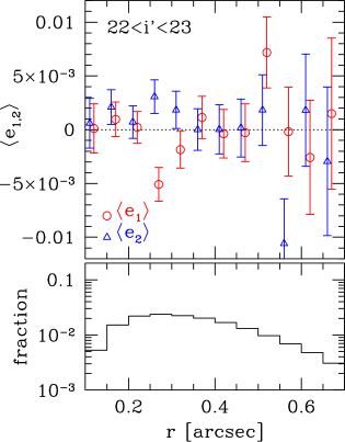
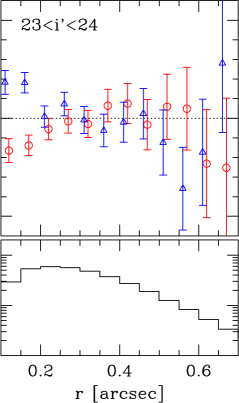
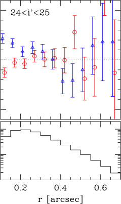
Figure 3: Top-panels: Mean ellipticities of galaxies as a function of semi-major axis desk scalelength in three $i^{\prime}$-band magnitude ranges. Open circles and triangles are for the $e_{1}$ and $e_{2}$ component of the galaxy ellipticities, respectively, obtained from lensfit model-fitting. Bottom-panels: The weighted galaxy fraction for each magnitude-scalelength grid.

It is known that galaxy shears estimated by lensfit are affected by multiplicative and additive bias, which are usually represented by (Heymans et al. 2012), $e^{\rm obs}=(1+m)[\gamma+e^{\rm int}]+c$. Miller et al. (2013) used realistic image simulations to estimate the multiplicative bias in CFHTLenS data, and found a size- and $S/N$-dependent bias with an average value of 6 percent. They derived the fitting function of the multiplicative bias [equation (14) of Miller et al. (2013)] that we employ for the current study. Using the fitting function, we evaluated an weighted average bias over source galaxies and found $\langle m\rangle=-0.059$. It is not clear whether the fitting function that was derived using mock CFHTLenS simulation data is applicable to the SuprimeCam data. We may, however, say that this does not seriously affect our results for the following two reasons: First, we don’t use a lensing induced quantity (shear or convergence) directly, but use the signal-to-noise ratio map of the lensing convergence (the convergence map normalized by its noise map). Therefore, our primary observational quantity, the peak counts, is not affected by the mutiplicative bias (see the next section). We, however, need to take the multiplicative bias into account in making the theoretical prediction of the peak counts. In order to do this, we will make a crude bias correction utilizing the average value of $\langle m\rangle=-0.059$ (see §4.1 for details). Since the statistical error in the peak counts is estimated as about 50 percent (see §4.2), the uncertainty associated with the multiplicative bias should be minor, that is the second reason.

Concerning the additive bias, we evaluated it in an empirical manner using weighted mean value of ellipticities over galaxies and found non-zero values with; $\langle c_{1}\rangle=\langle we_{1}^{\rm obs}\rangle=-0.00046\pm 0.00030$, and $\langle c_{2}\rangle=\langle we_{2}^{\rm obs}\rangle=0.0012\pm 0.00030$. In order to look into details of this, we computed the additive bias as a function of $i^{\prime}$-band magnitude and scalelength and found that the non-zero biases are mainly caused by faint-small galaxies as is shown in Fig. 3. This is in marked contrast to the result of CFHTLenS that the small-bright galaxies were found to be a cause of the significant additive bias in $\langle c_{2}\rangle$ (Heymans et al. 2012, note that their $\langle c_{1}\rangle=0.0001\pm 0.0001$ was found to be consistent with zero). The cause of these non-zero bias is unknown, but those different trends for different data sets may suggest that it may be caused by any instrumental or data-dependent effect. Heymans et al. (2012) calibrated the bias in an empirical manner, but we don’t do it because of the following two reasons: The first is that we search for high peaks in weak lensing mass maps which are obtained from azimuthally averaged tangential galaxy shears with an axisymmetric kernel. In that operation, the additive bias is partly canceled out. The second is that we deal with very high peaks corresponding to $\gamma\gtrsim 0.08$, thus the additive bias with the above small amplitude does not have a significant impact on our results.

3 Weak lensing mass maps and high $S/N$ peaks

3.1 Weak lensing mass maps

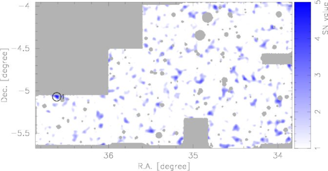
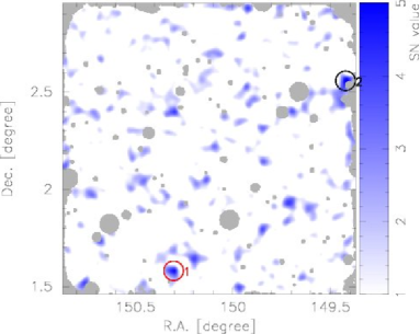
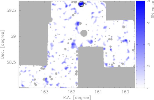
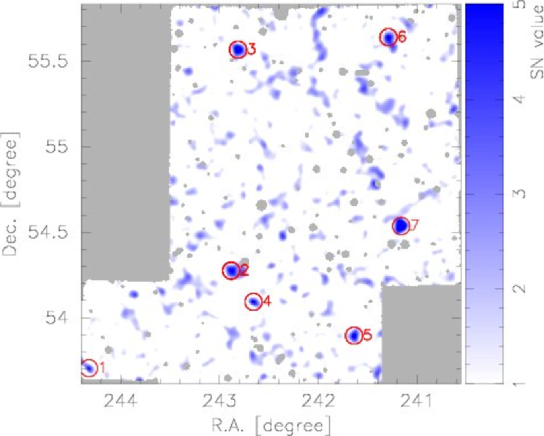
Figure 4: $\cal K$ maps for the XMM-LSS (top), COSMOS (middle-left), Lockman-hole (middle-right), and ELAIS-N1 (bottom) are shown by blue scale. Gray regions are either outside of data regions or masked regions where the data are affected by bright stars. High peaks with $S/N>4.5$ are marked with red circle along with ID given in Table  2. Black circles are for high peaks within the edge region.

The weak lensing mass map which is the smoothed lensing convergence field ($\kappa$) is evaluated from the tangential shear data by (Schneider 1996)

$${\cal K}(\mbox{\boldmath$\theta$})=\int d^{2}\mbox{\boldmath$\phi$}~{}\gamma_{t}(\mbox{\boldmath$\phi$}:\mbox{\boldmath$\theta$})Q(|\mbox{\boldmath$\phi$}|),$$ (1)

where $\gamma_{t}(\mbox{\boldmath$\phi$}:\mbox{\boldmath$\theta$})$ is the tangential component of the shear at position $\phi$ relative to the point $\theta$ and $Q$ is the filter function for which we adopt the truncated Gaussian function (for $\kappa$ field) (Hamana et al. 2012),

$$Q(\theta)={1\over{\pi\theta^{2}}}\left[1-\left(1+{{\theta^{2}}\over{\theta_{G}^{2}}}\right)\exp\left(-{{\theta^{2}}\over{\theta_{G}^{2}}}\right)\right],$$ (2)

for $\theta<\theta_{o}$ and $Q=0$ elsewhere. A nice property of this filter that should be noticed is that it has less power on the inner region ($\theta<\theta_{G}$, see Fig. 1 of Hamana et al. (2012)) thus a ${\cal K}$-peak resulting from a cluster of galaxies is less affected by contamination from cluster member galaxies.

In an actual computation, ${\cal K}$ is evaluated on regular grid points with a grid spacing of 0.15 arcmin using equation (1), but the integral in that equation is replaced with the summation over galaxies taking into account the lensing weight. The root-mean-square (RMS) noise coming from intrinsic ellipticity of galaxies (which we call the galaxy shape noise and denote by $\sigma_{\rm shape}$) is evaluated on each grid point in the following way: A “noise ${\cal K}$ map” is evaluated in the same way as the mass map but the orientation of galaxies is randomized. 1000 realizations of “noise ${\cal K}$ maps” are produced, and the RMS of 1000 ${\cal K}$ values is evaluated on each grid, which we take as the local estimate of $\sigma_{\rm shape}$. The signal-to-noise ratio of weak lensing mass map is defined by $S/N={\cal K}/\sigma_{\rm shape}$. The filter parameters should be chosen so that the $S/N$ is maximized for expected target clusters (i.e. $M>10^{14}h^{-1}M_{\odot}$ at $0.1<z<0.5$, see Hamana et al. (2004)). We take $\theta_{G}=1.5$ arcmin and $\theta_{o}=15$ arcmin. We show in Fig. 4 the ${\cal K}$-$S/N$ maps for four fields. Note that a ${\cal K}$-$S/N$ map is unaffected by the shear multiplicative bias ($m$) because we used the same galaxy ellipticity data for evaluating both the signal and noise, and thus the effect of the multiplicative bias is canceled out. Since in the following analysis we use only $S/N$ values, we did not correct for the shear multiplicative bias.

On and around regions where no source galaxy is available due to imaging data being affected by bright stars or large nearby galaxies, ${\cal K}$ may not be accurately evaluated. We define “data-region”, “masked-region” and “edge-region” by using the distribution of source galaxies as follows: First, for each grid, we check if there is a galaxy within 0.6 arcmin from the grid center. If there is no galaxy, then the grid is flagged as “no-galaxy”. After performing the procedure for all the grids, all the “no-galaxy” grids plus all the grids within 0.6 arcmin from all the “no-galaxy” grids are defined as the “masked-region”. All the grids located within 1.5 arcmin (we take this value by setting it equal to $\theta_{G}$) from any of “masked-region” grids are defined as the “edge-region”. All the rest of grids are defined as the “data-region”. Areas of four fields are summarized in Table 1. The total survey area (“data-region”+ “edge-region”) is 11.4 degree² with the “edge-region” accounting for 21 percent.

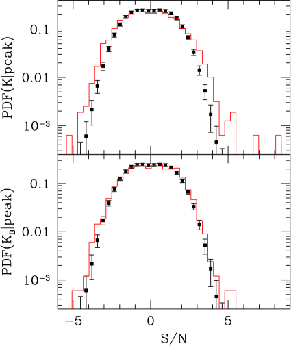
Figure 5: The probability distribution function of positive- and negative-curvature peaks (peaks and troughs) is shown. Top-panel is for $\cal K$ map, whereas bottom-panel is for the B-mode $\cal K$ map. The histogram shows the results from observed $\cal K$ and ${\cal K}_{B}$ maps. The points with error bars show the mean and RMS of PDF measured from 1000 random realizations of “noise ${\cal K}$ maps”, which represents the PDF expected for pure shape noise data.

Before looking into very high peaks, we examine statistical properties of peaks paying a special attention to an impact of residual systematics associated with data reduction and/or lensing shear measurement. We computed the probability distribution function of positive- and negative-curvature peaks (peaks and troughs) from the $\cal K$ maps, and plotted in Fig. 5. We also computed the PDFs expected for pure shape noise data using 1000 random realizations of “noise ${\cal K}$ maps”, and the mean and RMS of 1000 PDFs are also plotted in the figure. The upper panel of Fig. 5 shows the peak PDF measured from $\cal K$ maps, where clear deviations from pure shape noise PDF are seen. The deviations originate mainly from three sources: (1) massive clusters of galaxies that account for very high peaks (say $S/N>4.5$), (Miyazaki et al. 2002a; Hamana et al. 2004) which we shall go into details later, (2) cosmic large-scale structures which contribute to peaks at $S/N\lesssim 4.5$ (Maturi et al. 2010; Marian et al. 2010), and (3) residual systematics. In order to estimate the impact of the last one, we use the B-mode $\cal K$ map (${\cal K}_{B}$), which is the same smoothed convergence map as $\cal K$ but obtained from 45-degree rotated shear. In the standard gravity theory, only a small amount of B-mode lensing signal is produced (Schneider et al. 2002; Hilbert et al. 2009) which should be negligible for the current analysis. Since in the absence of lensing-induced B-mode signal, the ${\cal K}_{B}$-peak PDF should follow the pure shape noise PDF, it can be used for a diagnosis of residual systematics. It is found from the bottom panel of Fig. 5 that the ${\cal K}_{B}$-peak PDF deviates from the pure shape noise PDF, indicating existence of some residual systematics. Although a cause of the excess ${\cal K}_{B}$-peaks is unknown, it should be safer to consider that a similar amount of non-lensing-originated peaks may exist in the ${\cal K}$ maps. It can be also said from the ${\cal K}_{B}$ peak PDF that the probability of having a non-lensing-induced peak with $S/N>5$ is very rare. In addition to this fact, with a limited number of peaks with $S/N>5$, it is possible to inspect all the individual high peaks. Therefore we decided to use only the peaks with $S/N>5$ for our cosmological study in the next section. Understanding the origin of the excess ${\cal K}_{B}$ peak PDF must be a very important subject for future studies of weak lensing cluster counts using data from large surveys, however it is beyond the scope of this paper and we leave it for a future work.

3.2 High $S/N$ peaks

Table 2: Summary of high peaks with $S/N>4.5$.

Field - ID	R.A.	Dec.	Peak	flaga	Matched known clusters ($\theta_{\rm sep}<2$ arcmin)
	[deg]	[deg]	$S/N$		$\theta_{\rm sep}$b	$z_{p}$c	$z_{s,BCG}$d	Name and reference
XMM-LSS 1	36.6087	$-5.0671$	4.7	edge
COSMOS 1	150.3017	1.5838	4.8	-	$1.2^{\prime}$	0.36		#59 of (1)
					$1.5^{\prime}$	0.242		NSC J100113$+$013335(2)
					$1.5^{\prime}$	0.37		LSS 27 of (3)
					$1.9^{\prime}$	0.3610	0.3638	COSMOS CL J100112.4$+$013401(4)
COSMOS 2	149.4210	2.5585	5.1	edge	$0.5^{\prime}$	0.3787		WHL J095742.9$+$023332(5)
					$1.0^{\prime}$	0.17		LSS 36 of (3)
					$1.4^{\prime}$	0.362	0.3733	GMBCG J149.40425$+$02.57381(6)
					$1.4^{\prime}$	0.39		LSS 26 of (3)
Lockman-hole 1	161.6291	59.6266	7.6	edge	$0.7^{\prime}$	0.2317	0.2282	WHL J104625.5$+$593736(5)
					$1.0^{\prime}$	0.5672		SWIRE CL J104635.5$+$593732(4)
ELAIS-N1 1	244.2695	53.6936	4.6	-	$1.8^{\prime}$	0.9061		SWIRE CL J161710.9$+$534217(4)
ELAIS-N1 2	242.8739	54.2766	5.2	-	$0.5^{\prime}$	0.3794		NSC J161132$+$541649(2)
					$0.8^{\prime}$			SWIRE CL J161130.1$+$541704(4)
					$0.9^{\prime}$	0.3307		WHL J161135.9$+$541634(5)
ELAIS-N1 3	242.8169	55.5667	6.7	-	$0.8^{\prime}$	0.2246		SWIRE CL J161118.8$+$553431(4)
					$1.1^{\prime}$	0.2156		WHL J161121.1$+$553308(5)
					$1.8^{\prime}$			ZwCl 1610.0$+$5543(7)
ELAIS-N1 4	242.6503	54.0947	5.1	-	$1.0^{\prime}$	0.3786	0.3370	SWIRE CL J161045.2$+$540635(4)
					$1.2^{\prime}$	0.3618		2XMM J161040.5$+$540638(8)
ELAIS-N1 5	241.6525	53.8947	5.3	-	$0.2^{\prime}$	0.3432	0.3505	SWIRE CL J161045.2$+$540635(4)
					$0.7^{\prime}$	0.348		GMBCG J241.67338$+$53.89618(6)
ELAIS-N1 6	241.2632	55.6340	5.3	-	$0.1^{\prime}$	0.25385		MaxBCG J241.26104$+$55.63254(9)
					$1.0^{\prime}$	0.275		WHL J160503.4$+$553703(5)
					$1.2^{\prime}$	0.2299		NSC J160459$+$553700(2)
ELAIS-N1 7	241.1661	54.5305	8.2	-	$0.2^{\prime}$	0.2483		WHL J160439.4$+$543136(5)

^a Flag for edge regions (see §3.1 for the definition of the edge region).
^b Separation between the $\cal K$ peak and the cluster position given in the references.
^c Photometric redshift of clusters given in the references.
^d Spectroscopic redshift of BCG cluster given in the references.
Reference list: ⁽¹⁾Finoguenov et al. (2007), ⁽²⁾Gal et al. (2003), ⁽³⁾Scoville et al. (2007), ⁽⁴⁾Wen & Han (2011), ⁽⁵⁾Wen et al. (2009), ⁽⁶⁾Hao et al. (2010), ⁽⁷⁾Zwicky et al. (1961), ⁽⁸⁾Takey et al. (2011), ⁽⁹⁾Koester et al. (2007).

$\cal K$-peaks with $S/N>4.5$ are marked with open circles in Fig. 4, and are summarized in Table 2. We searched known cluster database taken from a compilation by NASA/IPAC Extragalactic Database (NED) for possible luminous baryonic counterparts within 2 arcmin from peak positions, and matched clusters of galaxies are also presented in Table 2. Most of the matched known clusters were identified by galaxy concentration in optical/infrared multi-band data and photometric redshifts of the clusters were evaluated. For some cases the spectroscopic redshifts of the brightest cluster galaxy (BCG) were measured. It turns out that all but XMM-LSS 1, which has the peak height of $S/N=4.7$ and is located in “edge-region”, have matched known clusters. Although for some peaks, matched clusters are located at slightly discrepant positions ($\theta_{\rm sep}>1$ arcmin), all the peaks with $S/N>5$ located in the “data-region” have a relatively well matched cluster of galaxies ($\theta_{\rm sep}\leq 1$ arcmin). Photometric redshifts of those closely matched counterparts are within the high lensing efficiency range ($0.1<z<0.5$), supporting an actual correspondence between galaxy over-density and high weak lensing signal. We thus conclude that the sample of $S/N>5$ peaks located in the “data-region” are not contaminated by a false signal, and we use the number counts of $N_{\rm peak}(S/N>5)=6$ in an effective area (“data-region” only) of 9.0 degree² for the cosmological study in the next section.

Figure 6: The probability distribution of the shape noise $\sigma_{\rm shape}$ evaluated evaluated on each grid point using 1000 realizations of “noise ${\cal K}$ maps” as described in §3.1. The mean and RMS of this distribution are found to be $\langle\sigma_{\rm shape}\rangle=0.017$ and RMS$(\sigma_{\rm shape})=0.0016$, respectively.

4 Constraints on the cosmological parameters and $M-c$ relation

Here we place constraints on the cosmological parameters ($\sigma_{8}$ and $\Omega_{m}$) and the mass–concentration ($M-c$) relation using the measured number counts of weak lensing clusters. To this end, we compare the measured counts with the theoretical model in the standard $\chi^{2}$ method. Below, we first describe the theoretical model of weak lensing cluster counts, then next we evaluate the error in the measured number counts which consist of the Poisson error and the cosmic variance, and finally we present results.

4.1 Theoretical model of weak lensing peak counts

We adopt the theoretical model of the weak lensing peak counts developed in Hamana et al. (2012), which is based on halo models. We refer the reader to the above reference for details of model and its comparison with mock numerical simulations. In short, the model is constructed under the assumption that high peaks are dominated by lensing signals from single massive haloes, for which it is assumed that the density profile is described by the truncated NFW model (Navarro et al. 1997; Baltz et al. 2009) and mass function is given by the model of Warren et al. (2006). Effects of intrinsic galaxy shape, the diversity of dark matter distributions within haloes, and large-scale structures are included in approximate approaches which were tested against the mock numerical simulations. Model parameters that should be specified for making the theoretical prediction of the weak lensing cluster counts are the cosmological parameters, $M-c$ relation of the dark matter haloes, the shape noise $\sigma_{\rm shape}$, and the redshift distribution of source galaxies. Below we will describe them in turn.

We treat $\Omega_{m}$ and $\sigma_{8}$ as free parameters, and fix the other cosmological parameters as follows: Hubble parameter $h=0.7$, the cosmological constant $\Omega_{\Lambda}=1-\Omega_{m}$, the baryon density $\Omega_{b}=0.051$, and the spectral index $n=0.96$, which are all consistent with the recent CMB experiments (Hinshaw et al. 2013; Planck Collaboration et al. 2014).

For the $M-c$ relation, we assume the following form,

$$c_{\rm vir}(M_{\rm vir},z)=c_{0}\left({{M_{\rm vir}}\over{10^{12}h^{-1}M_{\odot}}}\right)^{-0.075}(1+z)^{-0.7},$$ (3)

which is motivated by the findings from dark matter N-body simulations by Duffy et al. (2008); Macciò et al. (2008); Klypin et al. (2011); Prada et al. (2012), but we treat the normalization as a free parameter. Klypin et al. (2011) found $c_{0}=9.6$ for the cosmological model with $\Omega_{m}=0.27$ and $\sigma_{8}=0.82$. However, it should be noted that the mass–concentration relationship is known to be dependent on the cosmological model (Macciò et al. 2008; Zhao et al. 2009; Kwan et al. 2013; Diemer & Kravtsov 2015).

The peak $\cal K$ value from a halo is computed by assuming the tangential shear profile of a truncated NFW halo convolved with the smoothing function, eq. (2). Then it is converted to $S/N$ by specifying the shape noise, $\sigma_{\rm shape}$. Since $\sigma_{\rm shape}$ depends on the number density of source galaxies, it fluctuates depending on position. As we have described in §3.1, we evaluated $\sigma_{\rm shape}$ on each grid of weak lensing mass maps. We computed the probability distribution of the shape noise, which is presented in Fig. 6. The distribution is not very widely spread: its mean and RMS are found to be $\langle\sigma_{\rm shape}\rangle=0.017$ and RMS$(\sigma_{\rm shape})=0.0016$, respectively. We take this effect into account in the following way,

$$N_{\rm peak}(S/N)=\int d\sigma_{\rm shape}P(\sigma_{\rm shape})N_{\rm peak}(S/N;\sigma_{\rm shape}),$$ (4)

where $N_{\rm peak}(S/N;\sigma_{\rm shape})$ is the theoretical prediction of the weak lensing cluster number counts for a fixed $\sigma_{\rm shape}$ and $P(\sigma_{\rm shape})$ is the probability distribution function. Note that $\sigma_{\rm shape}$ measured from the data is affected by the multiplicative bias in shear measurement (§2.2). In order to take it into account, we calibrate the shape noise RMS by $\tilde{\sigma}_{\rm shape}=\sigma_{\rm shape}/(1-\langle m\rangle)$, and $P(\tilde{\sigma}_{\rm shape})$ with the measured distribution function shown in Fig. 6 is used to evaluate eq. 4.

Figure 7: Redshift distribution of galaxies used for the weak lensing mass reconstruction derived adopting the COSMOS photometric redshift catalog (Ilbert et al. 2009). The solid curve shows the fitting model by equation (8) with the parameters denoted in the panel.

In order to infer the redshift distribution of source galaxies, we utilized the COSMOS field data. We merged the source galaxy catalog used for the weak lensing mass reconstruction with the public COSMOS photometric redshift catalog (Ilbert et al. 2009), and computed the redshift distribution by adopting the photometric redshift. The derived redshift distribution is presented in Fig. 7. We fit the redshift distribution with the following function (Fu et al. 2008):

$$n_{s}(z)=A{{z^{a}+z^{ab}}\over{z^{b}+z^{c}}},$$ (5)

where the normalization, $A$, was determined by imposing $\int dz~{}n_{s}(z)=1$ within the integration range $0<z<6$. We found that a parameter set $(a,b,c)=(0.4,5.5,1.5)$ gives a reasonably good fit to the data, as shown in Fig. 7. The mean redshift of the model is 1.10 which is in very good agreement with the value derived from the photometric redshift data (1.09). In order to examine the variation in the redshift distribution due to the difference in the exposure time, we divide the COSMOS field into two subfields: one is the central region ($\sim 0.5$ degree²) where the exposure time is longer than 3,600 sec (with a median of 4,920 sec), and the other is the outer region where the exposure time is shorter than 3,600 sec (but mostly 2,400 sec) (see Taniguchi et al. 2007, for variation of the limiting magnitude). We computed the redshift distributions of those two samples separately, and found that the distributions are nearly indistinguishable, with mean redshifts of 1.093 and 1.090 for the inner-deep and outer-shallow samples, respectively. This may be partly due to our selection criteria that $i^{\prime}<25$ [AB mag], detection $S/N>8$ and FWHM larger than the stellar FWHM, which may result in rejection of small and faint distant galaxies. According to this finding and the fact that the redshift information for the other three fields is not available, we do not consider a possible field-to-field variation in the redshift distribution but use eq. (5) for computation of the theoretical prediction.

Figure 8: The probability distribution function of the number counts of peaks with $S/N>5$ found in 9.0 degree² fields. The distribution is derived from 10,000 realizations randomly taken from the full-sky mock weak lensing data. The mean and RMS of the distribution is 7.03 and 3.26, respectively.

4.2 Uncertainty in the number counts

In order to evaluate the uncertainty in the weak lensing cluster counts, we utilize mock weak lensing data generated from full-sky gravitational lensing ray-tracing simulations. Details of the simulation are given in Shirasaki, Hamana & Yoshida (2015 in prep.), here we describe only aspects that are directly relevant for this work. We adopted the cosmological model with $\Omega_{m}=0.278$, $\Omega_{\Lambda}=0.722$, $\sigma_{8}=0.82$, $h=0.70$ and $n=0.97$. These parameters are consistent with the WMAP nine-year results (Hinshaw et al. 2013). Gravitational lensing ray-tracing was performed through the dark matter distribution generated by the $N$-body simulations. In order to cover full-sky up to $z>1$, we combined, in a nested structure, 8 simulation boxes of different sizes with box side length from 450$h^{-1}$Mpc to 3,600$h^{-1}$Mpc. The $N$-body simulations were run with $2048^{3}$ dark matter particles using the parallel Tree-Particle Mesh code Gadget2 (Springel 2005). Light ray paths and the magnification matrix were evaluated by the multiple-plane ray-tracing algorithm of Teyssier et al. (2009) and Becker (2013). We used HEALPix pixelization of a sphere (Górski et al. 2005). The angular resolution parameter $nside$ was set to 8192. The corresponding angular resolution is $0.43$ arcmin. We adopted a fixed source redshift of $z_{s}=1.09$. On each pixel center, we computed the lensing shear. We added a random galaxy shape noise drawn from the truncated two-dimensional Gaussian to the lensing shear data (Hamana et al. 2012). The $\sigma$ of the Gaussian function was determined so that the shape noise in the resultant $\cal K$ map became equal to the mean observed value (after calibration with the multiplicative bias), that is $\tilde{\sigma}_{\rm shape}=\sigma_{\rm shape}/(1-\langle m\rangle)=0.018$. We adopted the same smoothing function as the actual measurement, eq. (2), and computed $\cal K$ from the noise-added shear data. Since we used the dark matter distribution from cosmological $N$-body simulations, the influence of large-scale structures on weak lensing cluster counts should be properly included.

Having generated the mock $\cal K$ data, we count the number of peaks with the threshold of $S/N>5$ in a contiguous 9.0 degree² region, which is randomly taken from the full-sky simulation data. We repeat this counting 10,000 times, allowing overlap in regions between different realizations. The probability distribution function of the resulting number counts is shown in Fig. 8. The mean and RMS of the distribution was found to be 7.03 and 3.26, respectively. Note that the solid curve in Fig. 8 represents the Gaussian distribution with the same mean and RMS, demonstrating that the measured distribution can be reasonably approximated by the Gaussian distribution. We may safely assume that the RMS consists of Poisson error and cosmic variance. Taking into account the difference between the observed number counts of 6 and the mean number counts of 7.03, we adopt $\sigma_{N}=3.1$ for the error in the observed weak lensing cluster counts, and thus we finally have $N_{\rm peak}=6\pm 3.1$.

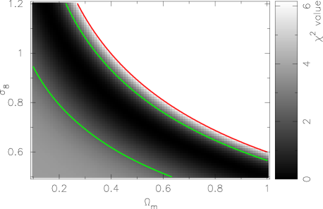
Figure 9: Constraints on $\Omega_{m}$ and $\sigma_{8}$ derived from the weak lensing cluster counts. Here the normalization of the $M-c$ relation is assumed to be $c_{0}=9.6$ (Klypin et al. 2011). Gray scale shows the $\chi^{2}$ with the inner green and outer red (upper limit only) contours indicating 68.3% ($\chi^{2}=2.30$), 95.4% ($\chi^{2}=6.17$) confidence levels, respectively.

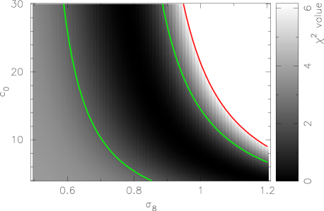
Figure 10: Same as Fig. 9 but on the $\sigma_{8}$ and $c_{0}$. Here the density parameter was fixed with $\Omega_{m}=0.278$.

Figure 11: Constraint on a single parameter $c_{0}$ derived from the weak lensing cluster counts. Here $\Omega_{m}$ and $\sigma_{8}$ are fixed to be the best fitting model of either the Planck (solid curve Planck Collaboration et al. 2014) or WMAP 9-year (dashed curve; Hinshaw et al. 2013).

4.3 Results

In order to place constraints on cosmological parameters and the $M-c$ relation using weak lensing cluster counts, we compare the measured counts with the theoretical prediction utilizing the standard $\chi^{2}$ method. Note that the resulting $\chi^{2}$ value does not represent the goodness-of-fit, as we have only one observed value, $N_{\rm peak}=6\pm 3.1$. Thus we use the $\chi^{2}$ value only for placing a confidence region on parameter spaces, adopting confidence levels assuming a normal distribution. We treat $\Omega_{m}$, $\sigma_{8}$ and $c_{0}$ as free parameters. Constraints obtained from the weak lensing cluster counts have degeneracy between those parameters (Mainini & Romano 2014; Cardone et al. 2014). However, since we have only one observed value with poor statistics, we do not explore the three-parameter space, but we examine two-parameter space, fixing one remaining parameter.

Figure 9 shows the derived constraint on $\Omega_{m}-\sigma_{8}$ plane. Here we did not treat $c_{0}$ as a fitting parameter but adopted the value ($c_{0}=9.6$) found from dark matter $N$-body simulations by Klypin et al. (2011) in which the $\Lambda$CDM model with $\Omega_{m}=0.27$ and $\sigma_{8}=0.82$ was employed. Therefore the constraint mainly comes from the cosmology dependence of the dark matter halo mass function with a minor contribution from the cosmology dependent lensing efficiency. Accordingly, the constraint exhibits the $\Omega_{m}-\sigma_{8}$ degeneracy in a similar fashion to X-ray cluster counts (Borgani et al. 2001; Henry 2004; Vikhlinin et al. 2009; Böhringer et al. 2014).

Figure 10 shows the derived constraint on the $\sigma_{8}-c_{0}$ plane, where the density parameter was fixed with $\Omega_{m}=0.278$. The degeneracy in the $\sigma_{8}-c_{0}$ space results from two relationships: one is increasing dark matter halo number density for larger $\sigma_{8}$, and the other is higher $S/N$-peak for larger $c_{0}$. Both of them result in larger weak lensing cluster counts. The upper limit on $c_{0}$ is hardly placed, because of the degeneracy in $\sigma_{8}-c_{0}$ and, for a given smoothing kernel, an excessively concentrated halo compared with the smoothing scale causes little variation in the peak height (Hamana et al. 2004). Although the current constraint does not even place a useful upper/lower limit on those parameters due to the poor statistics, this demonstrates that weak lensing cluster counts can be a useful probe of the cosmic structure formation scenario. The same argument, but based on a slightly different methodology, was already made by Liu et al. (2014b).

Finally, for a demonstrative purpose, we present in Figure 11, the constraint on a single parameter $c_{0}$ for two representative cosmological models: the Planck ($\Omega_{m}=0.315$, $\sigma_{8}=0.83$) (Planck Collaboration et al. 2014) and WMAP 9-year ($\Omega_{m}=0.278$, $\sigma_{8}=0.82$) (Hinshaw et al. 2013). It is obvious that the measured weak lensing cluster counts are consistent with the currently popular $\Lambda$CDM model. Specifically, the result from $N$-body simulations by Klypin et al. (2011) ($c_{0}=9.6$) is well within the 68.3% confidence region of both the Planck and WMAP9 cosmologies.

5 Summary and discussions

We presented the results of weak lensing cluster counts obtained from 11 degree² Subaru/SuprimeCam data. For the first time, we used the weak lensing cluster counts to place cosmological parameters and the mass–concentration relationship. In doing this, we explored, in an experimental manner, the capability and current issues of weak lensing cluster counts for cosmological studies.

The data were selected under the conditions that the exposure time longer than 1,800 sec along with the seeing condition of ${\rm FWHM}<0.7$ arcsec. These selection criteria result in the effective number density of galaxies usable for weak lensing shape measurement of $n_{g}\gtrsim 20$ arcmin^-2, which is about twice as large as those of previous works dealing with weak lensing peak statistics, namely, the CFHTLenS by Liu et al. (2014a) and CFHT Stripe-82 Survey by Liu et al. (2014b). Since the shape noise in the $\cal K$ map scales as $\sigma_{e}\propto n_{g}^{-1/2}$, higher galaxy density lifts up the peak height of a lensing signal of massive clusters. This allows us to adopt a high threshold $S/N$, in our case $S/N>5$. With high $S/N$, the contamination rate due to false signals is small, which enables us to construct a weak lensing-selected cluster sample.

We used lensfit for weak lensing shear measurement. We examined the additive bias in the measured galaxy ellipticities by evaluating weighted mean ellipticities as a function of galaxy size and magnitude. We found non-zero additive bias for both $e_{1}$ and $e_{2}$, which were found to be mainly caused by faint and small galaxies, as shown in Fig. 3. This is in marked contrast to the result of CFHTLenS in which small and bright galaxies were found to be a cause of additive bias in $e_{2}$ (Heymans et al. 2012). The cause of these non-zero biases is unclear, but those different trends for different data sets may suggest that it may be caused by some instrumental or data-dependent effect. We evaluated the amplitude of the multiplicative bias, adopting the empirical fitting function derived from CFHTLenS image simulations (Miller et al. 2013), and found the weighted average value of $\langle m\rangle=-0.059$. This does not have influence on the measured peak-$S/N$, as both the signal and noise RMS are affected in the same way, and thus those are canceled out. However, this must be properly taken into account in making the theoretical prediction. Since in the current study we considered the statistical quantity (peak counts), we adopted a statistical correction scheme that calibrating the shape noise RMS with the average bias factor $(1-\langle m\rangle)$.

We found 6 peaks with $S/N>5$. For all the peaks, previously identified clusters of galaxies are matched within a separation of $\theta_{\rm sep}<1$ arcmin. Most of the matched clusters were identified as a galaxy concentration in the sky and in multi-band color space of optical/infrared data. This provides us with a firm inspection of the purity of the weak lensing cluster sample. In fact, optical multi-band images are well suited to cross-identification, as the sensitivity of weak lensing mass map to cluster finding is most effective for clusters within the redshift range $0.1\lesssim z\lesssim 0.6$, where the red-sequence of cluster galaxies is located in optical color space. Thus, ongoing optical multi-band galaxy surveys with a single band observation being optimized for weak lensing shape measurement, namely the Kilo-Degree Survey (KiDS), Dark Energy Survey (DES), and Hyper-SuprimeCam (HSC) Survey (Miyazaki et al. 2012), may provide self-contained datasets for weak lensing cluster finding. Also, photometric redshifts will be estimated from multi-band data for each galaxy, which enable the source galaxy redshift distributions to be accurately determined.

We evaluated the statistical error in the weak lensing cluster counts using mock weak lensing data generated from full-sky ray-tracing simulations, and found $N_{\rm peak}=6\pm 3.1$. This error consists of the Poisson noise and the cosmic variance, with a larger contribution from the former.

We compared the measured weak lensing cluster counts with the theoretical model developed by Hamana et al. (2004, 2012), in which the effects of intrinsic galaxy shape, the diversity of dark matter distributions within haloes, and large-scale structures are included. Utilizing the standard $\chi^{2}$ method, we placed constraints on the $\Omega_{m}-\sigma_{8}$ plane, which was found to be consistent with currently standard $\Lambda$CDM models such as Planck model (Planck Collaboration et al. 2014) and WMAP 9-year model (Hinshaw et al. 2013), though the constraints are much broader than those CMB experiments due to the poor statistics ($N_{\rm peak}=6\pm 3.1$). It was demonstrated that the weak lensing cluster counts may place a unique constraint on $\sigma_{8}-c_{0}$ plane.

Finally we discuss prospects for ongoing/future surveys, taking the DES and HSC surveys as examples. Even taking into account a lower usable galaxy number density for those surveys, due to the shallower survey depth than this study, it may be feasible to obtain $N_{\rm peak}\sim 400$ clusters with $S/N\gtrsim 5$ (which can be achieved with $\sim 0.3$ peak/degree² for HSC survey of 1,400 degree², and $\sim 0.08$ peak/degree² for DES of 5,000 degree²). In that case, the error is dominated by the Poisson error and the expected fractional error will be $N_{\rm peak}^{-1/2}\sim 0.05$. This is 10 times better than the current study, $3.1/6\sim 0.5$. Therefore confidence regions become smaller and thus tighter constraints will be obtained; taking Figure 11 as an illustrative example, the corresponding 68.3% confidence level becomes $\chi^{2}=0.1$. This demonstrates that this methodology will be a useful probe of the cosmology and $M-c$ relation, though, in reality, marginalization over other parameters and degeneracy among parameters weaken constraints. More quantitative investigations of the capability of this method based on a Fisher analysis were made by Cardone et al. (2014); Mainini & Romano (2014). Having found that tight cosmological constraints can be achieved using the significantly improved statistics expected for ongoing/future surveys, it is necessary to check whether the theoretical model is correspondingly accurate, which is beyond the scope of this paper and is left for a future work.

We thank Y. Okura, M. Takada, M. Oguri and S. Miyazaki for useful discussions/comments. We are grateful to R. Takahashi and M. Shirasaki for assistance with running the $N$-body simulations for the full-sky gravitational lensing simulation. We would like to thank Matthew R. Becker for making the source codes of CALCLENS publicly available, and HEALPix team for HEALPix software publicity available. This paper makes use of software developed for the Large Synoptic Survey Telescope. We thank the LSST Project for making their code available as free software at http://dm.lsstcorp.org. We would like to thank HSC Data Analysis Software Team for their effort to develop hscPipe software suite. TH and LM thank the Aspen Center for Physics for their warm hospitality, where this work was partly done. Numerical computations in this paper were in part carried out Cray XC30 at Center for Computational Astrophysics, National Astronomical Observatory of Japan. This work is based in part on data collected at Subaru Telescope and obtained from the SMOKA, which is operated by the Astronomy Data Center, National Astronomical Observatory of Japan. This work is supported in part by Grant-in-Aid for Scientific Research from the JSPS Promotion of Science (23540324).

Appendix A Method of conversion from SIP to TPV

As described in §2, the instrumental distortion of images was corrected in the process of mosaic stacking along with astrometric calibration of CCD data using hscPipe in which the relationship between pixel coordinates and world coordinates systems (WCSs) is represented by SIP convention (Shupe et al. 2005). In lensfit, on the other hand, TPV convention is implemented. Here we describe the method for conversion of WCSs from SIP to TPV.

A.1 SIP convention

First, we summarize the SIP convention following Shupe et al. (2005). Let $u,v$ be relative pixel coordinates on a detector device with origin at CRPIX1, CRPIX2, and $x^{\prime},y^{\prime}$ be distortion corrected “intermediate world coordinates” in degree with origin at CRVAL1, CRVAL2. Then

$$\left(\begin{array}[]{c}x^{\prime}\\ y^{\prime}\end{array}\right)=\left(\begin{array}[]{cc}{\rm CD}1\_1&{\rm CD}1\_2\\ {\rm CD}2\_1&{\rm CD}2\_2\end{array}\right)\left(\begin{array}[]{c}u+f(u,v)\\ v+g(u,v)\end{array}\right),$$ (6)

where ${\rm CD}i\_j$ matrix encodes scaling, rotation and skew, and $f(u,v)$ and $g(u,v)$ are polynomial functions that represent distortion, given by

$$f(u,v) = \sum_{i,j}{\rm A}\_{i}\_{j}~{}u^{i}v^{j},\quad i+j\leq{\rm\tt A\_ORDER},$$ (7)

$$g(u,v) = \sum_{i,j}{\rm B}\_{i}\_{j}~{}u^{i}v^{j},\quad i+j\leq{\rm\tt B\_ORDER}.$$ (8)

In the standard SIP convention, A_ORDER and B_ORDER are allowed to range from 2 to 9.

A.2 TPV convention

Next, we summarize the TPV convention, in which relative pixel coordinates ($u,v$) are first converted to “distorted world coordinates” $(x,y)$ by

$$\left(\begin{array}[]{c}x\\ y\end{array}\right)=\left(\begin{array}[]{cc}{\rm CD}1\_1&{\rm CD}1\_2\\ {\rm CD}2\_1&{\rm CD}2\_2\end{array}\right)\left(\begin{array}[]{c}u\\ v\end{array}\right).$$ (9)

Then “intermediate world coordinates” $(x^{\prime},y^{\prime})$ can be given by polynomial functions of $x$ and $y$ as,

$$x^{\prime} = {\rm PV}{1}\_{0}~{}+{\rm PV}{1}\_{1}~{}x+{\rm PV}{1}\_{2}~{}y+{\rm PV}{1}\_{3}~{}r$$ (10)

$$+{\rm PV}{1}\_{4}~{}x^{2}+{\rm PV}{1}\_{5}~{}xy+{\rm PV}{1}\_{6}~{}y^{2}$$

$$+{\rm PV}{1}\_{7}~{}x^{3}+{\rm PV}{1}\_{8}~{}x^{2}y+{\rm PV}{1}\_{9}~{}xy^{2}$$

$$+{\rm PV}{1}\_{10}~{}y^{3}+{\rm PV}{1}\_{11}~{}r^{3}+\cdots,$$

$$y^{\prime} = {\rm PV}{2}\_{0}~{}+{\rm PV}{2}\_{1}~{}y+{\rm PV}{2}\_{2}~{}x+{\rm PV}{2}\_{3}~{}r$$ (11)

$$+{\rm PV}{2}\_{4}~{}y^{2}+{\rm PV}{2}\_{5}~{}xy+{\rm PV}{2}\_{6}~{}x^{2}$$

$$+{\rm PV}{2}\_{7}~{}y^{3}+{\rm PV}{2}\_{8}~{}xy^{2}+{\rm PV}{2}\_{9}~{}x^{2}y$$

$$+{\rm PV}{2}\_{10}~{}x^{3}+{\rm PV}{2}\_{11}~{}r^{3}+\cdots,$$

where $r=\sqrt{x^{2}+y^{2}}$, and the TPV polynomial functions have odd-power terms of $r$. The polynomial order of TPV is defined up to 7th, thus there are $2\times 40$ PV$i$_$j$ coefficients including $2\times 4$ odd $r^{n}$-terms.

A.3 Conversion from SIP to TPV

We derive conversion equations from SIP coefficients to TPV coefficients. To do so, we limit the polynomial order of SIP (A_ORDER and B_ORDER) being equal to or less than 7th, because that of TPV is defined up to 7th.

We can set PV$i$_$j$ coefficients for $r^{n}$-terms zero, because there are no corresponding terms in SIP polynomials. Also, we can safely use the same origins of $(u,v)$ and $(x^{\prime},y^{\prime})$ coordinates for TPV as those for SIP, because we derive the same distortion polynomial models as those of SIP but in the different (TPV) convention (thus the same CRPIX1, CRPIX2, CRVAL1 and CRVAL2 can be used). Then, we can set ${\rm PV}{1}\_{0}~{}={\rm PV}{2}\_{0}~{}=0$ as there are no corresponding terms in SIP. In addition, utilizing redundant degree of freedom in TPV convention, we can safely take the same ${\rm CD}i\_j$ matrix as one of SIP.

Equating the SIP and TPV coefficients of each $u^{i}v^{j}$ terms by order-by-order, we have the following simultaneous equations: For the 1st order,

$$\left(\begin{array}[]{c}{\rm CD}1\_1\\ {\rm CD}1\_2\end{array}\right) = \left(\begin{array}[]{cc}{\rm CD}1\_1&{\rm CD}2\_1\\ {\rm CD}1\_2&{\rm CD}2\_2\end{array}\right)\left(\begin{array}[]{c}{\rm PV}{1}\_{1{}}\\ {\rm PV}{1}\_{2{}}\end{array}\right),$$ (18)

$$\left(\begin{array}[]{c}{\rm CD}2\_1\\ {\rm CD}2\_2\end{array}\right) = \left(\begin{array}[]{cc}{\rm CD}2\_1&{\rm CD}1\_1\\ {\rm CD}2\_2&{\rm CD}1\_2\end{array}\right)\left(\begin{array}[]{c}{\rm PV}{2}\_{1{}}\\ {\rm PV}{2}\_{2{}}\end{array}\right),$$ (25)

which can be inverted and can be solved as,

$$\left(\begin{array}[]{c}{\rm PV}{1}\_{1{}}\\ {\rm PV}{1}\_{2{}}\end{array}\right)=\left(\begin{array}[]{c}{\rm PV}{2}\_{1{}}\\ {\rm PV}{2}\_{2{}}\end{array}\right)=\left(\begin{array}[]{c}1\\ 0\end{array}\right).$$ (26)

These are a natural consequence of distortion polynomial functions of SIP convention being defined only for 2nd and higher order terms (see eqs. (6) and (7)). For the 2nd order, we have

$$\left(\begin{array}[]{c}{\rm A}\_{2}\_{0}~{}{\rm CD}1\_1+{\rm B}\_{2}\_{0}~{}{\rm CD}1\_2\\ {\rm A}\_{1}\_{1}~{}{\rm CD}1\_1+{\rm B}\_{1}\_{1}~{}{\rm CD}1\_2\\ {\rm A}\_{0}\_{2}~{}{\rm CD}1\_1+{\rm B}\_{0}\_{2}~{}{\rm CD}1\_2\end{array}\right)=$$ (30)

$${\footnotesize\left(\begin{array}[]{ccc}{\rm CD}1\_1^{2}&{\rm CD}1\_1{\rm CD}2\_1&{\rm CD}2\_1^{2}\\ 2{\rm CD}1\_1{\rm CD}1\_2&{\rm CD}1\_1{\rm CD}2\_2+{\rm CD}1\_2{\rm CD}2\_1&2{\rm CD}2\_1{\rm CD}2\_2\\ {\rm CD}1\_2^{2}&{\rm CD}1\_2{\rm CD}2\_2&{\rm CD}2\_2^{2}\\ \end{array}\right)}$$ (34)

$$\times\left(\begin{array}[]{c}{\rm PV}{1}\_{4{}}\\ {\rm PV}{1}\_{5{}}\\ {\rm PV}{1}\_{6{}}\end{array}\right),$$ (38)

and

$$\left(\begin{array}[]{c}{\rm A}\_{2}\_{0}~{}{\rm CD}2\_1+{\rm B}\_{2}\_{0}~{}{\rm CD}2\_2\\ {\rm A}\_{1}\_{1}~{}{\rm CD}2\_1+{\rm B}\_{1}\_{1}~{}{\rm CD}2\_2\\ {\rm A}\_{0}\_{2}~{}{\rm CD}2\_1+{\rm B}\_{0}\_{2}~{}{\rm CD}2\_2\end{array}\right)=$$ (50)

$${\footnotesize\left(\begin{array}[]{ccc}{\rm CD}2\_1^{2}&{\rm CD}2\_1{\rm CD}1\_1&{\rm CD}1\_1^{2}\\ 2{\rm CD}2\_1{\rm CD}2\_2&{\rm CD}2\_1{\rm CD}1\_2+{\rm CD}2\_2{\rm CD}1\_1&2{\rm CD}1\_1{\rm CD}1\_2\\ {\rm CD}2\_2^{2}&{\rm CD}2\_2{\rm CD}1\_2&{\rm CD}1\_2^{2}\\ \end{array}\right)}$$

$$\times\left(\begin{array}[]{c}{\rm PV}{2}\_{4{}}\\ {\rm PV}{2}\_{5{}}\\ {\rm PV}{2}\_{6{}}\end{array}\right).$$

In the same manner, one can derive simultaneous equations in matrix form for higher order terms. Therefore, TPV coefficients, ${\rm PV}{i}\_{j}~{}$, can be obtained by solving those simultaneous equations using the standard matrix inversion method. In an actual computation, we performed matrix inversion and multiplication numerically.

References

- Axelrod et al. (2010) Axelrod, T., Kantor, J., Lupton, R. H., & Pierfederici, F. 2010, in Society of Photo-Optical Instrumentation Engineers (SPIE) Conference Series, Vol. 7740, Society of Photo-Optical Instrumentation Engineers (SPIE) Conference Series, 15
- Baba et al. (2002) Baba, H., et al. 2002, in Astronomical Society of the Pacific Conference Series, Vol. 281, Astronomical Data Analysis Software and Systems XI, ed. D. A. Bohlender, D. Durand, & T. H. Handley, 298
- Baltz et al. (2009) Baltz, E. A., Marshall, P., & Oguri, M. 2009, J. Cosmology Astropart. Phys, 1, 15
- Bartelmann et al. (2001) Bartelmann, M., King, L. J., & Schneider, P. 2001, A&A, 378, 361
- Becker (2013) Becker, M. R. 2013, MNRAS, 435, 115
- Bellagamba et al. (2011) Bellagamba, F., Maturi, M., Hamana, T., Meneghetti, M., Miyazaki, S., & Moscardini, L. 2011, MNRAS, 413, 1145
- Bertin (2006) Bertin, E. 2006, in Astronomical Society of the Pacific Conference Series, Vol. 351, Astronomical Data Analysis Software and Systems XV, ed. C. Gabriel, C. Arviset, D. Ponz, & S. Enrique, 112
- Bertin & Arnouts (1996) Bertin, E., & Arnouts, S. 1996, A&AS, 117, 393
- Bertin et al. (2002) Bertin, E., Mellier, Y., Radovich, M., Missonnier, G., Didelon, P., & Morin, B. 2002, in Astronomical Society of the Pacific Conference Series, Vol. 281, Astronomical Data Analysis Software and Systems XI, ed. D. A. Bohlender, D. Durand, & T. H. Handley, 228
- Böhringer et al. (2014) Böhringer, H., Chon, G., & Collins, C. A. 2014, A&A, 570, A31
- Borgani et al. (2001) Borgani, S., et al. 2001, ApJ, 561, 13
- Bullock et al. (2001) Bullock, J. S., Kolatt, T. S., Sigad, Y., Somerville, R. S., Kravtsov, A. V., Klypin, A. A., Primack, J. R., & Dekel, A. 2001, MNRAS, 321, 559
- Cardone et al. (2014) Cardone, V. F., Camera, S., Sereno, M., Covone, G., Maoli, R., & Scaramella, R. 2014, ArXiv e-prints
- Diemer & Kravtsov (2015) Diemer, B., & Kravtsov, A. V. 2015, ApJ, 799, 108
- Dietrich et al. (2012) Dietrich, J. P., Werner, N., Clowe, D., Finoguenov, A., Kitching, T., Miller, L., & Simionescu, A. 2012, Nature, 487, 202
- Duffy et al. (2008) Duffy, A. R., Schaye, J., Kay, S. T., & Dalla Vecchia, C. 2008, MNRAS, 390, L64
- Ettori et al. (2013) Ettori, S., Donnarumma, A., Pointecouteau, E., Reiprich, T. H., Giodini, S., Lovisari, L., & Schmidt, R. W. 2013, Space Sci. Rev., 177, 119
- Fan et al. (2010) Fan, Z., Shan, H., & Liu, J. 2010, ApJ, 719, 1408
- Finoguenov et al. (2007) Finoguenov, A., et al. 2007, ApJS, 172, 182
- Fu et al. (2008) Fu, L., et al. 2008, A&A, 479, 9
- Gal et al. (2003) Gal, R. R., de Carvalho, R. R., Lopes, P. A. A., Djorgovski, S. G., Brunner, R. J., Mahabal, A., & Odewahn, S. C. 2003, AJ, 125, 2064
- Gavazzi & Soucail (2007) Gavazzi, R., & Soucail, G. 2007, A&A, 462, 459
- Górski et al. (2005) Górski, K. M., Hivon, E., Banday, A. J., Wandelt, B. D., Hansen, F. K., Reinecke, M., & Bartelmann, M. 2005, ApJ, 622, 759
- Hamana & Miyazaki (2008) Hamana, T., & Miyazaki, S. 2008, PASJ, 60, 1363
- Hamana et al. (2013) Hamana, T., Miyazaki, S., Okura, Y., Okamura, T., & Futamase, T. 2013, PASJ, 65, 104
- Hamana et al. (2012) Hamana, T., Oguri, M., Shirasaki, M., & Sato, M. 2012, MNRAS, 425, 2287
- Hamana et al. (2004) Hamana, T., Takada, M., & Yoshida, N. 2004, MNRAS, 350, 893
- Hao et al. (2010) Hao, J., et al. 2010, ApJS, 191, 254
- Hennawi & Spergel (2005) Hennawi, J. F., & Spergel, D. N. 2005, ApJ, 624, 59
- Henry (2004) Henry, J. P. 2004, ApJ, 609, 603
- Heymans et al. (2012) Heymans, C., et al. 2012, MNRAS, 427, 146
- Hilbert et al. (2009) Hilbert, S., Hartlap, J., White, S. D. M., & Schneider, P. 2009, A&A, 499, 31
- Hinshaw et al. (2013) Hinshaw, G., et al. 2013, ApJS, 208, 19
- Ilbert et al. (2009) Ilbert, O., et al. 2009, ApJ, 690, 1236
- Ivezic et al. (2008) Ivezic, Z., et al. 2008, ArXiv e-prints
- King & Mead (2011) King, L. J., & Mead, J. M. G. 2011, MNRAS, 416, 2539
- Kitching et al. (2008) Kitching, T. D., Miller, L., Heymans, C. E., van Waerbeke, L., & Heavens, A. F. 2008, MNRAS, 390, 149
- Klypin et al. (2011) Klypin, A. A., Trujillo-Gomez, S., & Primack, J. 2011, ApJ, 740, 102
- Koester et al. (2007) Koester, B. P., et al. 2007, ApJ, 660, 239
- Kubo et al. (2009) Kubo, J. M., Khiabanian, H., Dell’Antonio, I. P., Wittman, D., & Tyson, J. A. 2009, ApJ, 702, 980
- Kwan et al. (2013) Kwan, J., Bhattacharya, S., Heitmann, K., & Habib, S. 2013, ApJ, 768, 123
- Liu et al. (2014a) Liu, J., Petri, A., Haiman, Z., Hui, L., Kratochvil, J. M., & May, M. 2014a, ArXiv e-prints
- Liu et al. (2014b) Liu, X., et al. 2014b, ArXiv e-prints
- Ludlow et al. (2014) Ludlow, A. D., Navarro, J. F., Angulo, R. E., Boylan-Kolchin, M., Springel, V., Frenk, C., & White, S. D. M. 2014, MNRAS, 441, 378
- Macciò et al. (2008) Macciò, A. V., Dutton, A. A., & van den Bosch, F. C. 2008, MNRAS, 391, 1940
- Mainini & Romano (2014) Mainini, R., & Romano, A. 2014, J. Cosmology Astropart. Phys, 8, 63
- Mantz et al. (2010) Mantz, A., Allen, S. W., Rapetti, D., & Ebeling, H. 2010, MNRAS, 406, 1759
- Marian et al. (2010) Marian, L., Smith, R. E., & Bernstein, G. M. 2010, ApJ, 709, 286
- Maturi et al. (2010) Maturi, M., Angrick, C., Pace, F., & Bartelmann, M. 2010, A&A, 519, A23
- Maturi et al. (2005) Maturi, M., Meneghetti, M., Bartelmann, M., Dolag, K., & Moscardini, L. 2005, A&A, 442, 851
- Miller et al. (2013) Miller, L., et al. 2013, MNRAS, 429, 2858
- Miller et al. (2007) Miller, L., Kitching, T. D., Heymans, C., Heavens, A. F., & van Waerbeke, L. 2007, MNRAS, 382, 315
- Miyazaki et al. (2007) Miyazaki, S., Hamana, T., Ellis, R. S., Kashikawa, N., Massey, R. J., Taylor, J., & Refregier, A. 2007, ApJ, 669, 714
- Miyazaki et al. (2002a) Miyazaki, S., et al. 2002a, ApJ, 580, L97
- Miyazaki et al. (2012) Miyazaki, S., et al. 2012, in Society of Photo-Optical Instrumentation Engineers (SPIE) Conference Series, Vol. 8446, Society of Photo-Optical Instrumentation Engineers (SPIE) Conference Series, 0
- Miyazaki et al. (2002b) Miyazaki, S., et al. 2002b, PASJ, 54, 833
- Navarro et al. (1997) Navarro, J. F., Frenk, C. S., & White, S. D. M. 1997, ApJ, 490, 493
- Planck Collaboration et al. (2014) Planck Collaboration, et al. 2014, A&A, 571, A16
- Prada et al. (2012) Prada, F., Klypin, A. A., Cuesta, A. J., Betancort-Rijo, J. E., & Primack, J. 2012, MNRAS, 423, 3018
- Rhodes et al. (2007) Rhodes, J. D., et al. 2007, ApJS, 172, 203
- Rozo et al. (2010) Rozo, E., et al. 2010, ApJ, 708, 645
- Schirmer et al. (2007) Schirmer, M., Erben, T., Hetterscheidt, M., & Schneider, P. 2007, A&A, 462, 875
- Schneider (1996) Schneider, P. 1996, MNRAS, 283, 837
- Schneider et al. (2002) Schneider, P., van Waerbeke, L., & Mellier, Y. 2002, A&A, 389, 729
- Scoville et al. (2007) Scoville, N., et al. 2007, ApJS, 172, 150
- Shan et al. (2012) Shan, H., et al. 2012, ApJ, 748, 56
- Shupe et al. (2005) Shupe, D. L., Moshir, M., Li, J., Makovoz, D., Narron, R., & Hook, R. N. 2005, in Astronomical Society of the Pacific Conference Series, Vol. 347, Astronomical Data Analysis Software and Systems XIV, ed. P. Shopbell, M. Britton, & R. Ebert, 491
- Springel (2005) Springel, V. 2005, MNRAS, 364, 1105
- Takey et al. (2011) Takey, A., Schwope, A., & Lamer, G. 2011, A&A, 534, A120
- Taniguchi et al. (2007) Taniguchi, Y., et al. 2007, ApJS, 172, 9
- Teyssier et al. (2009) Teyssier, R., et al. 2009, A&A, 497, 335
- Vikhlinin et al. (2009) Vikhlinin, A., et al. 2009, ApJ, 692, 1060
- Warren et al. (2006) Warren, M. S., Abazajian, K., Holz, D. E., & Teodoro, L. 2006, ApJ, 646, 881
- Wen & Han (2011) Wen, Z. L., & Han, J. L. 2011, ApJ, 734, 68
- Wen et al. (2009) Wen, Z. L., Han, J. L., & Liu, F. S. 2009, ApJS, 183, 197
- Wittman et al. (2006) Wittman, D., Dell’Antonio, I. P., Hughes, J. P., Margoniner, V. E., Tyson, J. A., Cohen, J. G., & Norman, D. 2006, ApJ, 643, 128
- Zhao et al. (2009) Zhao, D. H., Jing, Y. P., Mo, H. J., & Börner, G. 2009, ApJ, 707, 354
- Zwicky et al. (1961) Zwicky, F., Herzog, E., Wild, P., Karpowicz, M., & Kowal, C. T. 1961, Catalogue of galaxies and of clusters of galaxies, Vol. I