Using member galaxy luminosities as halo mass proxies of galaxy groups

Abstract

Reliable halo mass estimation for a given galaxy system plays an important role both in cosmology and galaxy formation studies. Here we set out to find the way that can improve the halo mass estimation for those galaxy systems with limited brightest member galaxies been observed. Using four mock galaxy samples constructed from semi-analytical formation models, the subhalo abundance matching method and the conditional luminosity functions, respectively, we find that the luminosity gap between the brightest and the subsequent brightest member galaxies in a halo (group) can be used to significantly reduce the scatter in the halo mass estimation based on the luminosity of the brightest galaxy alone. Tests show that these corrections can significantly reduce the scatter in the halo mass estimations by $\sim 50\%$ to $\sim 70\%$ in massive halos depending on which member galaxies are considered. Comparing to the traditional ranking method, we find that this method works better for groups with less than five members, or in observations with very bright magnitude cut.

1. Introduction

In the current scenario of galaxy formation, galaxies are thought to be formed and reside in cold dark matter haloes. Studying the galaxy-halo connection observationally provides one with important information about the underlying processes in galaxy formation and evolution. In recent years great progress has been made in establishing the halo-galaxy link via the so called halo occupation models (Jing, Mo & Börner 1998; Mo, Mao & White 1999; Peacock & Smith 2000; Zheng et al.2007) and the conditional luminosity functions (Yang et al. 2003; van den Bosch et al. 2003; Cooray et al. 2006). This halo-galaxy connection can also be made directly using galaxy groups which are defined as sets of galaxies that reside in the same dark matter halo, as is done in Yang et al. (2005c,d), Collister & Lahav (2005), van den Bosch et al. (2005), Robotham (2006), Zandivarez et al. (2006), Weinmann et al. (2006a,b).

Numerous group catalogues have been constructed from galaxy redshift surveys, including the 2-degree Field Galaxy Redshift Survey (2dFGRS) (Eke et al. 2004; Yang et al. 2005a), the high-redshift DEEP2 survey (e.g., Crook et al.2007); and the Sloan Digital Sky Survey (SDSS) (e.g., Berlind et al. 2006; Yang et al. 2007; Tago et al. 2010; Nurmi et al. 2013), the Galaxy and Mass Assembly (GAMA) observations (e.g. Robotham et al. 2011) using different methods, ranging from the traditional friends-of-friends (FOF) algorithm, to the hybrid matched filter method (Kim 2002) and the “MaxBCG” method (Koester et al. 2007). Relevant to the present paper is the halo-based group finder developed by Yang et al. (2005a), which groups galaxies according to their common halos expected from the current CDM model. This group finder is suited to study the relation between galaxies and dark matter haloes over a wide dynamic range in halo mass, from rich clusters of galaxies to poor groups of galaxies, as tested with mock galaxy surveys, and has been applied to 2dFGRS (Yang et al. 2005a), SDSS DR2 (Weinmann et al. 2006a), DR4 and DR7 (Yang et al. 2007).

One of the key steps in the halo-based group finder is the estimation of halo masses of candidate galaxy groups. In general, the halo masses of a group can be estimated based on the velocity dispersion of their member galaxies. However, except for a small fraction of very rich groups with a large number of satellite galaxies (e.g., Carlberg et al. 1996; 1997), this method is not very reliable for small groups with only a few members. In general, stacking of satellite galaxies for given central galaxies are used to obtain their halo masses (e.g., Erickson et al. 1987; Zaritsky et al. 1993; McKay et al. 2002; Brainerd & Specian 2003; Prada et al. 2003; van den Bosch et al. 2004; Becker et al. 2007; Conroy et al. 2007; Norberg et al. 2008; More et al. 2009b, 2011; Li et al. 2012).

Group total luminosity (e.g. Yang et al. 2005a; 2007) or richness (e.g. Berlind et al. 2006; Becker et al. 2007; Andreon & Hurn 2010; Hao et al. 2010) can also be used as halo mass indicator. As demonstrated in Yang et al. (2007), the halo mass is tightly correlated with the total luminosity of member galaxies. Unfortunately not all member galaxies can be observed because galaxy samples are usually magnitude limited. In practice, one can only measure a characteristic group luminosity, $L_{G}$, which is defined as the total luminosity of member galaxies brighter than a given luminosity threshold. In the SDSS group catalogue of Yang et al., this luminosity threshold is chosen to be $\>{}^{0.1}{\rm M}_{r}-5\log h=-19.5$, so that one can reach to a depth of $z=0.09$. Here $\>{}^{0.1}{\rm M}_{r}-5\log h$ is the absolute $r$-magnitude, K- and E-corrected to $z=0.1$, the typical redshift of galaxies in the SDSS redshift sample. Assuming that $L_{G}$ increases monotonically with halo mass $M_{h}$, one can then obtain the halo masses of galaxy groups by abundance matching between groups and dark matter halos,

$$\int_{L_{G}}^{\infty}n_{G}(L_{G}^{\prime})dL_{G}^{\prime}=\int_{M_{h}}^{\infty}n_{h}(M_{h}^{\prime})dM_{h}^{\prime}\,,$$ (1)

where $n_{G}(L_{G})$ is the number density of groups at characteristic luminosity $L_{G}$, and $n_{h}(M_{h})$ is the halo mass function for the cosmology adopted. In Yang et al. (2007), $M_{h}-L_{G}$ relation so obtained is used iteratively in the group finder to link galaxies in the same dark matter halo, and to assign halo masses to individual galaxy groups.

As shown in Yang et al. (2005a; 2007) using mock galaxy catalogs, the halo based group finder and the mass assignment scheme work well for a moderately deep and large survey, such as the 2dFGRS and SDSS. However, the method may not work as well for shallow surveys, such as the 6dFGRS (Jones et al. 2009), and for groups selected from high redshift surveys, such as DEEP2 (Willmer et al. 2006), COSMOS (Ilbert et al. 2009) and GAMA (Driver et al. 2011) where only a few (in most cases one or two) brightest member galaxies are observed in each dark matter halo. In case the survey volume is very small or difficult to calculate because of the bad survey geometry, the halo mass estimation based on the ranking of $L_{G}$ may become unachievable. Moreover, there are also some catalogues which only consists of a certain type of galaxies, for example, the SDSS-III’s Baryon Oscillation Spectroscopic Survey (BOSS) (Dawson et al. 2013) which map the spatial distribution of luminous red galaxies (LRGs). It is unclear if the method can work well for those catalogues. Thus, an alternative estimate of the halo masses is required for such groups.

To estimate the halo masses for galaxy systems with only one or two brightest member galaxies, one may make use of the central-host halo relation obtained from conditional luminosity function (CLF; e.g. Yang et al. 2003; van den Bosch et al. 2003), the subhalo abundance matching (SHAM; e.g., Vale & Ostriker 2006), or from predictions of semi-analytical model (SAM; e.g., Kang et al. 2005). As shown in Yang et al. (2008) and Cacciato et al. (2009), the typical scatter in $\log L_{c}$ for halos of a given mass is about 0.15. However for massive halos $L_{c}\propto M_{h}^{\sim 0.25}$, and so the scatter in halo mass for a given $L_{c}$ can be substantial. Thus the central (or the brightest) galaxy alone can not provide a reliable estimation of the halo mass, especially for massive halos. Recently, suggestions have been made to the magnitude gap between the brightest and second brightest galaxies as another parameter to describe the halo mass in addition to $L_{c}$ (e.g., Hearin et al. 2013a; More 2012; Shen et al. 2014). In this paper, we investigate how halo masses are correlated with group properties, such as the central galaxy luminosity, the satellite member galaxy luminosity or the luminosity gap, defined as $\log L_{\rm gap}=\log L_{c}-\log L_{s}$, where $L_{s}$ is the luminosity of the i-th brightest member galaxies. For example, if a group only has two members, then $L_{s}$ is the luminosity of the second brightest galaxy. If a group contains five member galaxies, we choose to use the luminosity of the fifth brightest member galaxy. The goal of this paper is to improve the halo mass estimation using both $L_{c}$ and the luminosity gap. The investigations are carried out based on four mock samples generated using SAM, SHAM, and two CLF models, respectively.

The outline of this paper is as follows. §2 describes the four mock samples used in this paper that are constructed using the SAM, SHAM, and CLF, respectively. In §3 we present the relationships between the halo mass and the total group (or central galaxy) luminosity. In §3.3 we show how the luminosity gap affects the $L_{c}-M_{h}$ relation and can be used to reduce the scatter within this relation. In §3.4, we investigate the improvement of this reduction by involving more fainter member galaxies in calculating luminosity gap. In §4, we compare the performance of two halo mass estimation methods, which are based on luminosity gap (refer to ‘GAP’) and traditional ranking method (‘RANK’) under different circumstances, respectively. Finally, we summarize our results in §5.

2. samples of mock groups

In this paper, we make use of four sets of mock galaxy catalogs. The first is constructed by Guo et al. (2011; hereafter G11) using a semi-analytic model of galaxy formation applied to dark matter halo merging trees obtained from the ‘Millennium Run’ N-body simulation (Springel et al. 2005). The cosmological parameters adopted in the simulation are $\Omega_{m}=0.25$, $\Omega_{\Lambda}=0.75$, $h=0.73$ and a CDM spectrum with an amplitude specified by $\sigma_{8}=0.9$. This set of parameters is different from that obtained in recent observations (e.g. Planck Collaboration et al. 2013; Mandelbaum 2013). However, for our test of accuracy of halo mass assignment, this is not a big issue. The simulation was performed with GADGET2 (Springel 2005) using $2160^{3}$ dark matter particles in a periodic cubic box with a side length $L_{\rm box}=500\>h^{-1}{\rm{Mpc}}$ (in comoving units). The mass of a particle is $8.6\times 10^{8}\>h^{-1}\rm M_{\odot}$. In their modeling, G11 included the growth and activity of the central black holes, as well as their effects on suppressing the cooling and star formation in dark matter halos. Since we are interested in finding an accurate halo-mass proxy from observed luminosities, here we only use the halo mass and $r$-band luminosity of each galaxy given by G11. We refer the reader to G11 for the details of the semi-analytic model (see also in Guo et al. 2013). In this paper, we only make use of these galaxies with luminosity $\log L\gtrsim 8.0$. This set of mock galaxy catalog is referred to as ‘SAM’.

The second mock galaxy catalog is constructed by Hearin et al. (2013b). They used the Bolshoi N-body simulation (Klypin et al. 2011) which models the cosmological growth of structure in a cubic volume with side length $L_{\rm box}=250\>h^{-1}{\rm{Mpc}}$ within a standard $\Lambda$CDM cosmology with parameters: $\Omega_{m}=0.27$, $\Omega_{\Lambda}=0.73$, $h=0.7$, $n=0.95$ and $\sigma_{8}=0.82$. After utilizing the ROCKSTAR (Behroozi et al. 2012) halo finder to identify halos and subhalos, subhalo abundance matching (SHAM) technique was adopt to associate galaxies with dark matter halos. This technique, called as age distribution matching, is a two-phase algorithm for assigning both luminosity and color to the galaxies located at the center of halos (see Hearin et al. 2013a; 2013b for details). Here, we make use of their galaxy catalog in the cubic box that contains 244784 galaxies at redshift $z=0.1$ with $r$-band absolute magnitude $\>{}^{0.1}{\rm M}_{r}-5\log h<-19.0$.

The third mock galaxy sample used in this paper is constructed by populating dark matter halos obtained from numerical simulations with galaxies of different luminosities according to the conditional luminosity function (CLF; Yang et al. 2003). The algorithm of populating galaxies is similar to that outlined in Yang et al. (2004) but here updated to the CLF in $r$-band. The CLF, $\Phi(L|M_{h})$, is defined to be the average number of galaxies of luminosities $L\pm dL/2$ that reside in a halo of mass $M_{h}$ (see Yang et al. 2003). Here we give a brief description of the algorithm of assigning luminosity to each member galaxy. First, we write the total CLF as the sum of the CLFs of central and satellite galaxies (Yang et al. 2003; van den Bosch et al. 2003; Vale & Ostriker 2004, 2006; Cooray 2006; van den Bosch et al. 2007; Yang et al. 2008):

$$\Phi(L|M_{h})=\Phi_{\rm cen}(L|M_{h})+\Phi_{\rm sat}(L|M_{h})\,.$$ (2)

We assume the contribution from the central galaxies to be a lognormal distribution:

$$\Phi_{\rm cen}(L|M_{h})~{}d\log L~{}~{}~{}~{}~{}~{}~{}~{}~{}~{}~{}~{}~{}~{}~{}~{}~{}~{}~{}~{}~{}~{}~{}~{}~{}~{}~{}~{}~{}~{}~{}~{}~{}~{}~{}~{}~{}~{}~{}~{}~{}~{}~{}~{}~{}~{}~{}~{}~{}~{}~{}~{}~{}~{}~{}~{}~{}~{}~{}~{}$$ (3)

$$={1\over{\sqrt{2\pi}\sigma_{c}}}{\rm exp}\left[-{{(\log L-\log L_{c})^{2}}\over 2\sigma_{c}^{2}}\right]~{}d\log L\,,$$

where $\sigma_{c}$ is a free parameter, which expresses the scatter in $\log L$ of central galaxies at fixed halo mass, and $\log L_{c}$ is the expectation value for the (10-based) logarithm of the luminosity of the central galaxy. For the contribution from the satellite galaxies we adopt a modified Schechter function which decreases faster at the bright end than the Schechter function:

$$\Phi_{\rm sat}(L|M)~{}d\log L~{}~{}~{}~{}~{}~{}~{}~{}~{}~{}~{}~{}~{}~{}~{}~{}~{}~{}~{}~{}~{}~{}~{}~{}~{}~{}~{}~{}~{}~{}~{}~{}~{}~{}~{}~{}~{}~{}~{}~{}~{}~{}~{}~{}~{}~{}~{}~{}~{}~{}~{}~{}~{}~{}~{}~{}~{}~{}~{}~{}$$ (4)

$$=\phi^{*}_{s}\left({L\over L^{*}_{s}}\right)^{(\alpha_{s}+1)}{\rm exp}\left[-\left({L\over L^{*}_{s}}\right)^{2}\right]\ln(10)~{}d\log L\,.$$

The parameters $L_{c}$, $\sigma_{c}$, $\phi^{*}_{s}$, $\alpha_{s}$ and $L^{*}_{s}$ are all functions of the halo mass $M_{h}$.

Following Yang et al. (2008) and Cacciato et al. (2009), we assume that $\sigma_{c}$ is a constant independent of halo mass, and that the $L_{c}-M_{h}$ relation has the following functional form,

$$L_{c}(M_{h})=L_{0}\frac{(M_{h}/M_{1})^{\gamma_{1}}}{(1+M_{h}/M_{1})^{\gamma_{1}-\gamma_{2}}}\,.$$ (5)

This model contains four free parameters: a normalized luminosity, $L_{0}$, a characteristic halo mass, $M_{1}$, and two slopes, $\gamma_{1}$ and $\gamma_{2}$. For satellite galaxies we use

$$\log L^{*}_{s}(M_{h})=\log L_{c}(M_{h})-0.25\,,$$ (6)

$$\alpha_{s}(M_{h})=\alpha_{s}$$ (7)

(i.e., the faint-end slope of $\Phi_{\rm sat}(L|M_{h})$ is independent of halo mass), and

$$\log[\phi^{*}_{s}(M_{h})]=b_{0}+b_{1}(\log M_{12})+b_{2}(\log M_{12})^{2}\,,$$ (8)

with $M_{12}=M_{h}/(10^{12}h^{-1}\>{\rm M_{\odot}})$. This set of CLF parameterization thus has a total of nine free parameters, characterized by the vector

$${\lambda}^{\rm CLF}\equiv(\log M_{1},\log L_{0},\gamma_{1},\gamma_{2},\sigma_{c},\alpha_{s},b_{0},b_{1},b_{2})\,.$$ (9)

The above functional forms do not have ample physical motivations but were found to adequately describe the observational results obtained by Yang et al. (2008) from the SDSS galaxy group catalog. They were adopted in Cacciato et al. (2009) to make the model prediction for the galaxy-galaxy lensing signals, and very recently in van den Bosch et al. (2013), More et al. (2013) and Cacciato et al. (2013) to constrain both the CLF and cosmological parameters with the SDSS clustering and weak lensing measurements. Here we adopt the set of the best fit CLF parameters that are obtained for the Millennium simulation cosmology, with $(\log M_{1}=10.954,\log L_{0}=9.896,\gamma_{1}=5.192,\gamma_{2}=0.2415,\sigma_{c}=0.1501,\alpha_{s}=-0.6828,b_{0}=-0.1611,b_{1}=0.7945,b_{2}=-0.1573)$.

Galaxies with luminosities $\log(L/h^{-2}{\rm L}_{\odot})\gtrsim 8.0$ are populated in the dark matter halos extracted from the Millennium Simulation. In practice, each halo is assigned a central galaxy with a median luminosity specified by Eq. (5) and a log-normal dispersion $\sigma_{c}=0.1501$. The satellite galaxies are populated via following steps: (1) obtain the mean number of satellite galaxies according to the integration of Eq.(4) with luminosities $\log L\gtrsim 8.0$; (2) use a Possion distribution with the mean obtained in step (1) to obtain the number of satellite galaxies; (3) assign a luminosity to each of these satellite galaxy according to Eq.(4). Note that satellite galaxies are allowed to be brighter than the central galaxy. However, we note that in our subsequent analysis, following the observational definition, the central galaxy is defined as the brightest galaxy in a halo. We refer to this set of mock galaxy catalog as ‘CLF1’.

Finally, in order to test if our analysis is cosmological dependent or not, we construct another set of mock galaxy catalog which we call as ‘CLF2’. The cosmological parameters adopted for this set of mock galaxy catalog are those given by WMAP3: $\Omega_{m}=0.238$, $\Omega_{\Lambda}=0.762$, $h=0.73$, $n=0.95$ and $\sigma_{8}=0.75$. We adopt the set of the best fit CLF parameters that are consistent with WMAP3 cosmology, provided in Cacciato et al. (2009), with $(\log M_{1}=11.07,\log L_{0}=9.935,\gamma_{1}=3.273,\gamma_{2}=0.255,\sigma_{c}=0.143)$ (see Cacciato et al. 2009 for more details). Here again, we use the halo catalog from the ‘Millennium Run’ N-body simulation to construct the mock catalog. Since the cosmology adopted in the Millennium simulation is different from the WMAP3 cosmology, we scale the halo masses in the Millennium simulation to the WMAP3 cosmology using abundance matching according to the mass functions of WMAP3 cosmology and the Millennium simulation. Such abundance matching ignores the difference in the spatial correlations between halos in different cosmologies, but should be valid for our analysis which is based only on galaxy occupation in individual halos.

Among the above four mock catalogs, although the SAM has more ‘physics’ in it, but doesn’t really fit the data (e.g., see Weinmann et al. 2006; Liu et al. 2010; Nurmi et al. 2013), whereas the CLF1, CLF2 and SHAM mocks are not based on physical models of galaxy formation but do fit the observational data. Here in our subsequent probes, we make use of CLF1 as our fiducial sample, and take others mainly for comparisons.

3. Halo masses from luminosities of member galaxies

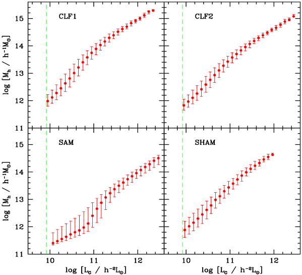
Figure 1.— The halo mass $M_{h}$ v.s. characteristic group luminosity $L_{G}$ in the CLF1 (top left panel), CLF2 (top right panel), SAM (bottom left panel) and SHAM (bottom right panel) mock catalogs. Here results are shown for the median (symbols) and 68% confidence level (error bars) of $\log M_{h}$ within each $\log L_{G}$ bin. The vertical green dashed line in each panel shows the luminosity limit at $\>{}^{0.1}{\rm M}_{r}-5\log h=-19.5$.

In order to carry out cosmological and structure formation investigations using observations of galaxy systems, one of the key steps is to obtain reliable estimations of the halo masses of the systems selected. The kinematics of member galaxies is one of the most commonly used methods to estimate masses of optically selected groups/clusters (e.g., van den Bosch et al. 2004; Kargert et al. 2004; More et al. 2011). However, this method may be significantly affected by anisotropies of the velocity dispersion (e.g. Biviano et al, 2006; White et al. 2010). Furthermore, for groups containing only a few members, or when only a few group members can be observed, the estimation of velocity dispersion becomes noisy, making the dynamical mass estimation unreliable.

Recently, another halo mass indicator has been used to estimate halo masses for galaxy systems over a large dynamical range. This method uses the richness or the characteristic group luminosity as the proxy of halo mass, and so can readily be applied once galaxy systems are selected from a redshift survey. Richness is one of the easiest quantities of a galaxy system to observe, but there are different ways to define the richness. For instance, one can define it as the number of member galaxies within the red sequence or above a certain luminosity threshold. Gladders & Yee (2000, 2005) used the red sequence richness to measure the mass of the halos from photometric data. The characteristic group luminosity (or stellar mass), which is defined as the total group luminosity (stellar mass) of member galaxies above a certain luminosity threshold, is presumably a better mass indicator than the richness. This is especially the case for very poor galaxy systems dominated by a single luminous galaxy, where the galaxy luminosity is known to change as a function of halo mass over a large range.

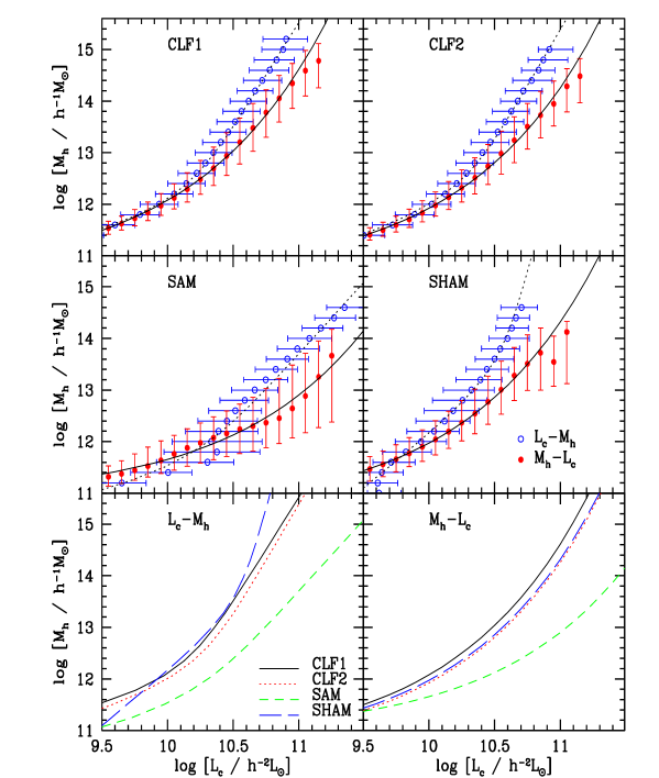
Figure 2.— The median halo mass, $M_{h}$, as function of central galaxy luminosity, $L_{c}$. The red solid circles show the median values of $M_{h}$ in given central galaxy luminosity bins. Error bars indicate the 68% confidence level around the median values. Here results are shown for mock samples CLF1 (top left), CLF2 (top right), SAM (middle left) and SHAM (middle right), respectively. The solid line in each panel is the best fit $M_{h}-L_{c}$ relation. As a comparison, we also show using blue open circles the median $\log L_{c}$ in different $\log M_{h}$ bins with horizontal error bars indicating the 68% confidence levels around the median. The dotted line in each panel is the best fit $L_{c}-M_{h}$ relation. The bottom two panels show all the fitting lines of $L_{c}-M_{h}$ relation (bottom left) and $M_{h}-L_{c}$ relation (bottom right) for four mock samples respectively.

3.1. Using the characteristic group luminosity

As demonstrated in Yang et al. (2005a; 2007) using mock redshift surveys, the total luminosity of all member galaxies in a group is tightly correlated with halo mass. This method needs the determination of the total group luminosity. However, a limitation of this method is the need of corrections in real observations where only bright galaxies are observed. Although one may make corrections using a luminosity function (e.g. that for the total galaxy population), detailed CLF modeling shows that the correction depends significantly on halo mass (Yang et al. 2003; van den Bosch et al. 2007; Yang et al. 2008). To avoid this uncertainty and as a compromise with observational magnitude limit, one may use a characteristic group luminosity, defined as the total luminosity of member galaxies above a luminosity threshold. For instance, Yang et al. (2005a; 2007) used a characteristic group luminosity, $L_{G}$, which is defined as the total luminosity of all group members brighter than ${}^{0.1}{\rm M}_{b_{J}}-5\log h=-18$ for the 2dFGRS group catalogue, or of all group members brighter than $\>{}^{0.1}{\rm M}_{r}-5\log h=-19.5$ for the SDSS DR7 group catalogue, as the halo mass proxy. Tests using mock galaxy and group catalogues show that the characteristic group luminosity is tightly correlated with the mass of the dark matter halo hosting the group (Yang et al. 2005a). Once the characteristic group luminosities of all the groups are obtained, one can assign groups with halo masses according to abundance matching (e.g. Mo, Mao & White 1999) between the group luminosity function and the halo mass function predicted with a given cosmology (see Yang et al. 2007 for details).

Fig. 1 shows the relation between the characteristic group luminosity $L_{G}$ (the total luminosity of all group members brighter than $\>{}^{0.1}{\rm M}_{r}-5\log h=-19.5$) and the halo mass $M_{h}$ obtained directly from the CLF1, CLF2, SAM and SHAM mock galaxy catalogs in different panels as indicated, respectively. The symbols in each panel are the median values while the error-bars are the 1-$\sigma$ variation (68% confidence level). There is a clear tight correlation between the characteristic luminosity and the halo mass. The typical 1-$\sigma$ variations in $\log M_{h}$ given by the SAM sample are $\sim 0.2$ for massive halos and $\sim 0.4$ for intermediate mass ($M_{h}\sim 10^{12.5}\>h^{-1}\rm M_{\odot}$) halos. The corresponding variations given by the CLF1, CLF2 and SHAM samples are $\sim 0.1$ for massive halos and $\sim 0.3$ in the intermediate mass range. Note that, the very asymmetric error bars at low luminosity end for SAM sample are caused by a combination of the color modeling of central galaxies in halos around $10^{11.8}\>h^{-1}\rm M_{\odot}$ (see Fig. 2 for such a feature for central galaxies), the luminosity cut at $\>{}^{0.1}{\rm M}_{r}-5\log h=-19.5$ and a smaller bin size used here.

3.2. Using the brightest (central) galaxy

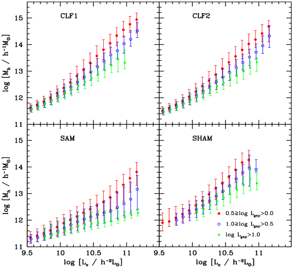
Figure 3.— Similar to the results shown in Fig. 2, but here for groups within three different luminosity gap ranges: $0.5\geq\log L_{\rm gap}>0.0$ (solid circles), $1.0\geq\log L_{\rm gap}>0.5$ (open circles) and $\log L_{\rm gap}>1.0$ (solid squares). Here again, symbols and error bars represent the median and 68% confidence levels of $\log M_{h}$ in different $\log L_{c}$ bins.

In the local Universe, the characteristic group luminosities can be determined for groups down to a halo mass of $\sim 10^{12}\>h^{-1}\rm M_{\odot}$ with surveys like the 2dFGRS and the SDSS. However, if one goes to higher redshift or uses much shallower observations (e.g. 6dFGRS), where only a few brightest members a group can be observed, corrections for the missing members have to be made to obtain the characteristic group luminosity, making the method unreliable. On the other hand, investigations with the CLF model and observed group and cluster catalogues have shown that the luminosity of the central galaxy $L_{c}$ of a group is correlated with its halo mass $M_{h}$ (e.g., Yang et al. 2003; van den Bosch et al. 2003; Yang et al. 2007). As an illustration, Fig.2 shows the model predictions of the $L_{c}-M_{h}$ relation from the four mock samples described in Section 2 as marked in each panel, respectively. In each panel, the blue open circles are the median values of the central galaxy luminosity in different halo mass bins, and the horizontal error bars show the 68% confidence level around the median luminosities. As one can see, the median luminosity of central galaxy increases monotonically with halo mass, and that the amounts of scatter are comparable among four mock catalogs. For reference, we fit the $L_{c}-M_{h}$ relations using the functional form given by Eq. (5). The fitting parameters are listed in Table 1 and the best fitting results are shown in Fig. 2 with the dotted lines. For the CLF1 and CLF2 samples, the parameters are adopted the same as those listed in Section 2. These fitting formulae describe the median $L_{c}-M_{h}$ relations remarkably well. For the most massive halos, the SAM predicts central galaxies are significantly brighter than the CLF model. However, as compared among SAMs and SDSS observations in G11, the stellar mass functions at massive end of SAMs do not show very significant deviation, the above difference may due to the color modeling of these galaxies. Their model central galaxies, especially in $\sim 10^{11.8}\>h^{-1}\rm M_{\odot}$ halos, tend to be too blue and bright. This is the case of the wiggle in their $M_{h}-L_{c}$ relation and the resulting much smaller median $L_{c}-M_{h}$ relation.

Table 1Parameters for the $L_{c}-M_{h}$ relation

Sample	$\log L_{0}$	$\log M_{1}$	$\gamma_{1}$	$\gamma_{2}$
CLF1	9.896	10.954	5.192	0.2415
CLF2	9.935	11.07	3.273	0.255
SAM	10.02$\pm$0.25	10.95$\pm$0.48	2.59$\pm$0.40	0.36$\pm$0.03
SHAM	10.25$\pm$0.16	12.94$\pm$0.56	0.36$\pm$0.03	0.22$\pm$0.03

Although the $L_{c}-M_{h}$ relations presented above are useful in predicting the luminosities of central galaxies in halos of given masses, these relations are not appropriate for estimating halo mass from $L_{c}$. Because the luminosity function is steep at the bright end, and because the scatter in the $L_{c}(M_{h})$ relations is quite large, $M_{h}$ will be over-estimated from the $L_{c}(M_{h})$ relation due to a Malmquist-like bias. In order to have an unbiased result, we need to obtain the $M_{h}(L_{c})$ relation directly instead of using the inverse of the $L_{c}(M_{h})$ relation. In Fig. 2 we plot the median (red solid circles) and the 68% confidence levels (error bars) of halo masses, $\log M_{h}$, as a function of central galaxy luminosity $\log L_{c}$, obtained directly from the CLF1, CLF2, SAM and SHAM samples. Here again the median halo mass increases monotonically with the central galaxy luminosity. For low-mass halos, the median of the $M_{h}(L_{c})$ relation is similar to that of the $L_{c}(M_{h})$ relation, but for halos with mass $M_{h}>10^{12}\>h^{-1}\rm M_{\odot}$ these two relations are quite different, exactly because of the Malmquist-like bias. The scatter in $\log M_{h}$ for a given luminosity increases with $\log L_{c}$, and at the bright end is much larger than that in the $L_{c}(M_{h})$ relation, particularly in the SAM prediction, clearly due to the shallow slope in the $L_{c}(M_{h})$ relation (for example, $L_{c}\propto M_{h}^{\sim 0.25}$ at the massive end for the CLF sample) (see More et al. 2009a; 2009b for more detailed discussions). On the other hand, as pointed out in More et al. (2009b), the huge scatter in $M_{h}$ at large $L_{c}$ seen in SAM is inconsistent with the constraints obtained using satellite kinematics. We fit the median $M_{h}(L_{c})$ relations with the following functional form:

$$\log M_{h}=\exp(\log L_{c}-\log M_{a})+\log M_{b}\,.$$ (10)

The best fitting parameters of $[\log M_{a},\log M_{b}]$ are: $[9.61\pm 0.01,10.60\pm 0.01]$ for the CLF1 sample, $[9.69\pm 0.02,10.56\pm 0.03]$ for the CLF2 sample, $[10.32\pm 0.03,10.93\pm 0.04]$ for SAM sample and $[9.68\pm 0.02,10.64\pm 0.03]$ for SHAM sample, respectively. The resulting best fit median relations are shown in Fig. 2 as the solid lines. Note that the above fitting formula are obtained within the halo mass range shown in the plot, extrapolation to much larger halo mass is not valid. For clarity, we put all the fitting lines of four mock samples in the bottom two panels for $L_{c}-M_{h}$ relations on the right and $M_{h}-L_{c}$ relations on the left. Obviously, for SAM, both relations are inconsistent with the other three mock samples. As we have mentioned before, it’s because the galaxy luminosity in SAM model is overestimated compare to the other three mock samples.

The above results show that the scatter in the $M_{h}(L_{c})$ is quite large at the massive end. It is therefore not a good choice to use $L_{c}$ alone as a halo mass proxy. On the other hand, we see in Fig. 1 that the scatter shown for a given characteristic group luminosity is much smaller, which indicates that using additional member galaxies can give better constrain of the halo masses. In what follows we investigate how to get a better halo mass proxy by using the luminosities of other brightest member galaxies.

3.3. Using the brightest two galaxies

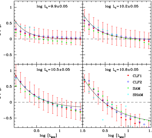
Figure 4.— The halo mass difference, $\Delta\log M_{h}$, between the best fit $M_{h}-L_{c}$ relation and data as a function of luminosity gap $\log L_{\rm gap}$. The results shown in different panels are for central galaxies within different luminosity bins: $\log L_{c}=9.9\pm 0.05$ (upper-left), $10.2\pm 0.05$ (upper-right), $10.5\pm 0.05$ (lower-left) and $10.8\pm 0.05$ (lower-right), respectively. In each panel, red solid circles are results obtained from the CLF1 sample, where the symbols and error bars represent the median and 68% confidence levels of $\Delta\log M_{h}$. Black solid line is the best fitting results to the data from CLF1 sample. The results obtained from CLF2, SAM and SHAM samples are also shown in each panel for comparison using different symbols as indicated.

To start with, we introduce a ‘luminosity gap’, defined as the luminosity ratio between the central and a satellite galaxy in the same dark matter halo, $L_{\rm gap}=L_{c}/L_{s}$. In this section, we focus on the brightest satellite galaxy, so that $L_{s}=L_{2}$, where $L_{2}$ is the luminosity of the brightest satellite or the second brightest among all the member galaxies. Recent studies have shown that this luminosity gap may contain important information about halo mass (e.g., Hearin et al. 2013; More 2012). As found in Shen et al. (2014), $L_{2}$ is also correlated with group richness which, in turn, is correlated with halo mass. Thus a combination of the luminosities of the brightest and second brightest galaxies in a halo is likely to provide more information regarding the halo mass than the brightest galaxy alone.

The luminosity gap $L_{\rm gap}$ can be measured straightforwardly for groups/halos that have at least two members. Within our four samples, the distribution of the luminosity gap, $\log L_{\rm gap}$, spreads roughly in the range 0.0-3.0. We split each of our mock group catalogues into three subsamples according to the value of $\log L_{\rm gap}$: small gap groups with $0.5\geq\log L_{\rm gap}>0.0$; median gap groups with $1.0\geq\log L_{\rm gap}>0.5$; and large gap groups with $\log L_{\rm gap}>1.0$. Fig. 3 shows the same $M_{h}(L_{c})$ relations as shown in Fig. 2, but separately for each of the gap subsamples, as indicated by different symbols. Clearly, groups with different amounts of luminosity gap have distinctive $M_{h}(L_{c})$ relations, especially at the massive end. For the same central galaxy luminosity, groups with a smaller luminosity gap (or larger $L_{2}$) tends to be more massive, especially for groups whose central galaxy luminosities are larger than $10^{10.0}\,h^{-2}\rm L_{\odot}$. For fainter central galaxies, the $M_{h}(L_{c})$ relations are similar for the three luminosity gaps, due to the small scatter in the halo mass - central galaxy luminosity relation. We may notice the much larger reduction of error bars at bright central luminosity end for large gap groups with $\log L_{\rm gap}>1.0$ in SAM mock sample. This is also due to the fact that in SAM the luminosities of central galaxies in a large number of low mass groups are overestimated compared to the other three mock samples. As we mentioned before, this overestimation of luminosity may come from the incorrect color modeling of these galaxies.

The strength of the luminosity-gap dependence increases monotonically with the central galaxy luminosity. All these suggest that the luminosity gap can be used to reduce the scatter in the $M_{h}-L_{c}$ relations, particularly at the massive end.

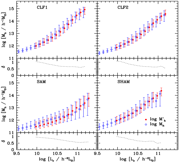
Figure 5.— Similar to the results shown in Fig. 2, but here we compare the original (open circles) $\log M_{h}$ and luminosity gap pre-corrected (solid circles) $\log M^{\prime}_{h}$ halo masses. Obviously, the latter has significantly reduced scatters in $\log M_{h}$, especially at the massive end. The ratio between these two error bars, $\delta$, are shown in the small panels with dashed lines.

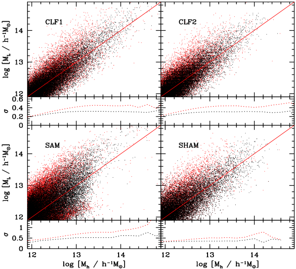
Figure 6.— Comparison to the true halo mass for four mock samples. Red points are halo masses obtained using Eq. 10, while black points are obtained using Eq. 11. Red solid lines show the relation when $\log M_{L}$ equals to $\log M_{h}$. The standard variance of galaxies from the red solid lines, $\sigma$, are shown in the small panels. The red dotted line corresponds to red points of the above panels, while black one corresponds to black points.

To model halo mass using also luminosity gap, we formally write

$$\log M_{h}(L_{c},L_{\rm gap})=\log M_{h}(L_{c})+\Delta\log M_{h}(L_{c},L_{\rm gap})\,,$$ (11)

where the first term on the right side is the empirical relation described by Eq. (10), while $\Delta\log M_{h}(L_{c},L_{\rm gap})$ represents the amount of correction to the $M_{h}(L_{c})$ relation with the help of $L_{\rm gap}$. Fig. 4 shows the relation between luminosity gap and $\Delta\log M_{h}$ for given central galaxy luminosity, where $\Delta\log M_{h}$ is defined by the ratio between the true halo mass and that predicted by eq. (10). Shown in different panels are for halos (groups) in different $L_{c}$ bins, centered at $\log L_{c}=9.9$, 10.2, 10.5, 10.8, with a bin width equal to 0.1, respectively.

The red solid points represent the median $\Delta\log M_{h}$ for each luminosity gap subsamples constructed from the CLF1 sample, with error bars indicating the 68 percentile. In all cases $\Delta\log M_{h}$ decreases with increasing luminosity gap, consistent with the trend seen in Fig 3, where one sees that halos with a smaller luminosity gap are more massive. The overall amplitude of $\Delta\log M_{h}$ increases with the central luminosity, consist with the growing sizes of errorbars at the large $L_{c}$ end shown in Fig. 2. For different $L_{c}$ the asymptotic values of $\Delta\log M_{h}$ are also different.

We use the following functional form to model $\Delta\log M_{h}(L_{c},L_{\rm gap})$,

$$\Delta\log M_{h}(L_{c},L_{\rm gap})=\eta_{a}\exp(\eta_{b}\log L_{\rm gap})+\eta_{c}\,,$$ (12)

where parameters $\eta_{a}$, $\eta_{b}$ and $\eta_{c}$ may all depend on $L_{c}$. The parameter $\eta_{b}$ in general has a negative value which describes the decline rate of $\Delta\log M_{h}$ with $\log L_{\rm gap}$. Parameter $\eta_{c}$ describes the asymptotic value at large $\log L_{\rm gap}$, while parameter $\eta_{a}+\eta_{c}$ is the value of $\Delta\log M_{h}$ at $\log L_{\rm gap}=0$. To gain some idea of the functional forms of these three parameters, we first fit to the data for each of the $\log L_{c}$ bins shown in Fig. 4, and obtain the values of $\eta_{a}$, $\eta_{b}$ and $\eta_{c}$. According to their general dependence on $\log L_{c}$, we use the following forms to model these three parameters as functions of $\log L_{c}$:

$$\eta_{a}(L_{c})~{} = ~{}\exp(\log L_{c}-\beta_{1})$$

$$\eta_{b}(L_{c})~{} = ~{}\alpha_{2}(\log L_{c}-\beta_{2})\,,$$ (13)

$$\eta_{c}(L_{c})~{} = ~{}-(\log L_{c}-\beta_{3})^{\gamma_{3}}$$

which in total has five free parameters. We fit all the data for CLF1 (as shown partly in Fig. 4) in the luminosity range $10.9\geq\log L_{c}\geq 9.7$ with the above model using a Monte-Carlo Markov Chain (MCMC) to explore the likelihood function in the multi-dimensional parameter space (see Yan, Madgwick & White 2003; van den Bosch et al. 2005b for more detail). Then, we chose the parameter set has the highest likelihood (minimum $\chi^{2}$) to be the model parameters. The best fit values together with their 68% confidence ranges are listed in the first row of Table 2. This set of parameter values are valid for central galaxies in the luminosity range $10.9\geq\log L_{c}\geq 9.7$. For central galaxies outside this range, one can apply the correction factor at $\log L_{c}=9.7$ for fainter galaxies and $\log L_{c}=10.9$ for brighter galaxies. At the faint end, the asymptotic correction factor $\Delta\log M_{h}$ at $\log L_{c}=9.7$ is small. At the bright end, the reason to cut at $\log L_{c}=10.9$ is that our data for massive halos are statistically poor and not included in the fitting and that the fitting function for the $M_{h}(L_{c})$ relation (Eq. 10) starts to deviate from data at $\log L_{c}>10.9$.

Table 2Parameters for the $\Delta\log M_{h}$ function

$\Delta\log M_{h}$	$\beta_{1}$	$\alpha_{2}$	$\beta_{2}$	$\beta_{3}$	$\gamma_{3}$
MEMBER 2	$10.37^{+0.23}_{-0.25}$	$2.14^{+4.22}_{-1.81}$	$-11.57^{+0.64}_{-6.40}$	$9.90^{+0.02}_{-0.16}$	$3.29^{+4.13}_{-1.54}$
MEMBER 3	$10.09^{+0.16}_{-0.19}$	$0.25^{+1.50}_{-0.15}$	$-16.51^{+5.29.46}_{-6.62}$	$9.86^{+0.04}_{-0.20}$	$2.92^{+2.00}_{-1.12}$
MEMBER 4	$9.84^{+0.15}_{-0.22}$	$0.15^{+0.71}_{-0.07}$	$-16.70^{+5.18}_{-3.90}$	$9.69^{+0.10}_{-0.21}$	$2.82^{+0.87}_{-0.63}$
MEMBER 5	$9.71^{+0.13}_{-0.18}$	$0.10^{+0.43}_{-0.02}$	$-17.74^{+6.07}_{-0.16}$	$9.60^{+0.10}_{-0.19}$	$2.75^{+0.76}_{-0.35}$
MEMBER 6	$9.57^{+0.11}_{-0.24}$	$0.07^{+0.29}_{-0.01}$	$-18.02^{+6.14}_{-0.39}$	$9.49^{+0.10}_{-0.24}$	$2.77^{+0.40}_{-0.26}$
MEMBER 7	$9.78^{+0.13}_{-0.30}$	$-0.89^{+0.75}_{-0.70}$	$-9.59^{+2.39}_{-0.25}$	$9.80^{+0.10}_{-0.40}$	$2.64^{+1.59}_{-0.74}$
MEMBER 8	$9.53^{+0.33}_{-0.12}$	$-0.28^{+0.13}_{-1.10}$	$-8.84^{+1.00}_{-1.00}$	$9.47^{+0.43}_{-0.16}$	$2.55^{+1.02}_{-0.50}$
MEMBER 9	$9.91^{+0.11}_{-0.20}$	$0.07^{+0.05}_{-0.01}$	$-16.78^{+2.46}_{-0.46}$	$9.38^{+0.07}_{-0.14}$	$2.63^{+0.19}_{-0.18}$

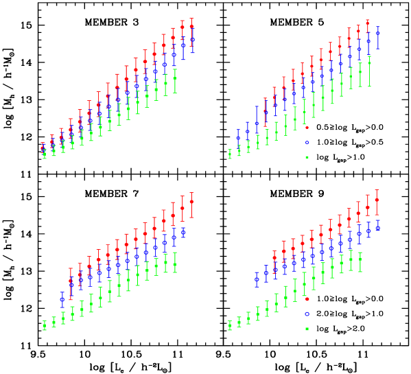
Figure 7.— Similar to the results shown in Fig. 3, but here for CLF1 mock sample with three, five, seven and nine brightest member galaxies been observed and used in calculating the luminosity gap. Groups within three different luminosity gap ranges are shown using different symbols as indicated in the upper and lower right panels. Here again, symbols and error bars represent the median and 68% confidence levels of $\log M_{h}$ in different $\log L_{c}$ bins.

The best fit $\Delta\log M_{h}$ as a function of $\log L_{\rm gap}$ is shown in each panel of Fig. 4 as the solid line. Obviously, the model describes the overall behavior in $\Delta\log M_{h}(L_{c},L_{\rm gap})$ remarkably good. For comparison, we also show $\Delta\log M_{h}(L_{c},L_{\rm gap})$ as a function of $\log L_{\rm gap}$ obtained from the CLF2, SAM and SHAM samples in each panel of Fig.4 using different symbols as indicated. Although coming from completely different galaxy formation models and/or cosmological parameters, the halo mass correction factors for other samples are quite similar to that for the CLF1 sample. Such agreement indicates that our model for $\Delta\log M_{h}(L_{c},L_{\rm gap})$ is quite insensitive to the details of galaxy formation and cosmology.

Since the main purpose of this paper is to obtain a better halo mass estimator, we compare the amount of scatter in the original $\log M_{h}(L_{c})$ relation and the new $\log M_{h}(L_{c},L_{\rm gap})$ model. To perform such a comparison, we define a ‘pre-corrected’ halo mass

$$\log M^{\prime}_{h}=\log M_{h}-\Delta\log M_{h}(L_{c},L_{\rm gap})\,,$$ (14)

and check if the scatter in the $M^{\prime}_{h}(L_{c})$ relation is significantly reduced relative to that in the $M_{h}(L_{c})$. If the correction were perfect, the scatter in the $M^{\prime}_{h}(L_{c})$ would be reduced to 0.

Fig. 5 demonstrates the performance of the corrected model. Here results for the original $M_{h}(L_{c})$ relations are shown as the open circles and the $M^{\prime}_{h}(L_{c})$ relation as the solid points. The error-bars are all 68 percentiles around the median values in the $L_{c}$ bins. It is clear that the scatter in $M^{\prime}_{h}(L_{c})$ is significantly reduced relative to the original relation, especially for massive halos/groups where the scatter is reduced by about 50%. For clarity, we define the ratio between the corrected and original error bars as $\delta$ in the sub-panels. We can see, $\delta$ close to 1.0 at low mass ends indicate that two error bars is about the same. Then $\delta$ drop to about 0.5 for four samples show that the corrected error bar can reduce 50% of the original one. Note that the correction model $\Delta\log M_{h}$ is calibrated by the CLF1 sample alone, but its application to other samples also leads to significant reduction in the scatter. These results indicate clearly that adding of even just the second brightest galaxy can give a significant improvement of the mass estimation over using the central (the brightest) galaxy alone.

In order to further test the reliability of this halo mass estimation, we compared the halo mass $\log M_{L}$ obtained from the galaxy luminosity using Eq. 11 to the true halo mass $\log M_{h}$ for each group which are directly available in our four mock samples: CLF1 CLF2, SAM and SHAM galaxy catalogs. Fig. 6 shows this comparison. The red points represent the halo masses estimated using only $L_{c}$, i.e., using Eq. 10. While the black points represent the halo masses estimated using both $L_{c}$ and $L_{\rm gap}$ (Eq. 11). In order to quantify the scatter with respect to the line of equality ($\log M_{L}=\log M_{h}$) in each panel, we measure the standard variance $\sigma$ between estimated and true halo mass for each galaxy group. The $\sigma$ is defined as:

$$\sigma=\sqrt{\frac{\sum_{i=1}^{n}(\log M_{h}-\log M_{L})^{2}}{n-1}}\,,$$ (15)

where $n$ is the number of groups in each halo mass bin with width $\Delta\log M_{h}=0.1$. The results, shown in the small panels, with red dotted lines represent the standard variance for only using $L_{c}$ and black ones represent the estimation by using both $L_{c}$ and $L_{\rm gap}$, indicate that the estimations for halo mass are all improved for four mock samples. Overall, adding the second brightest member galaxy can roughly reduce the scatter by $\sim 0.3$dex at the massive end.

We also noticed that the halo masses estimated using $L_{c}$ alone has somewhat systematical deviation from the true halo masses at the massive end. Here the systematic deviation is mainly induced by the so called Eddington bias where there are significantly more low mass halos than massive halos that can scattered to larger ones. As we can see, with the help of the second brightest member galaxy, this deviation decreases substantially. And we will see later that using additional member galaxies, such systematic deviation indeed disappears finally.

3.4. Using subsequent member galaxies

Having demonstrated that the luminosity gap between central and the brightest satellite galaxy can be used to better constrain the halo mass estimation, we come to subsequent member galaxies. Since the richness is also an indicator for halo mass and correlated with $L_{c}$ (Shen et al. 2014), we may expect the luminosity gap between central and the other satellite galaxies also contains information of halo mass. In this subsection, we will extend our study to fainter member satellite galaxies. Like before, we still use the ‘luminosity gap’ $L_{gap}=L_{c}/L_{s}$, but here $L_{s}$ is the luminosity of $i$-th member galaxy in consideration with $L_{s}=L_{3}$ or $L_{4}$, etc., where $L_{3}$ and $L_{4}$ are the luminosities of the third and fourth brightest galaxies in this group. Note that, in general one can also define $L_{s}$ as the total luminosity of all member satellite galaxies in consideration. However, as we have tested, this definition dose not improve any of our results. While the gap thus defined has negative values. For simplicity, we adopt $L_{s}$ as luminosity of the $i$-th brightest member galaxy.

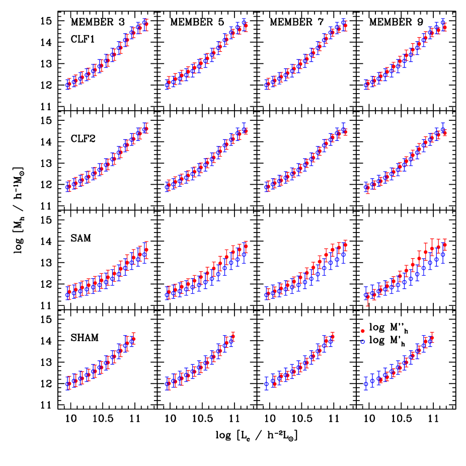
Figure 8.— Similar to the results shown in Fig. 5 but here for four mock samples (CLF1, CLF2, SAM and SHAM from top to bottom rows) with three, five, seven and nine brightest members galaxies been observed and used in calculating the luminosity gap. Here we compare the luminosity gap pre-corrected (open circles) halo mass $\log M^{\prime}_{h}$ (the second brightest galaxy) in Fig. 5 with the ones obtained from the third, fifth, seventh and ninth brightest member galaxies, respectively. Obviously, the latter make further reduction on scatters in $\log M^{\prime\prime}_{h}$, especially at the massive end.

We start with the third brightest member galaxy and stop at the ninth. For the fainter member galaxy, the luminosity gap will be larger. Overall, the values of $L_{gap}$ are roughly in the range $0.0-3.0$. As before, we split groups into three categories according to the value of the luminosity gap. The separation criteria for groups with member less than five are: small gap ($0.5\geq\log L_{\rm gap}>0.0$), median gap ($1.0\geq\log L_{\rm gap}>0.5$) and large gap ($\log L_{\rm gap}>1.0$). The criteria for groups with six and more member galaxies are: small gap ($1.0\geq\log L_{\rm gap}>0.0$), median gap ($2.0\geq\log L_{\rm gap}>1.0$) and large gap ($\log L_{\rm gap}>2.0$). As an illustration, we show in Fig. 7 the gap-dependent halo mass distributions, here for CLF1 sample only. From top left to right bottom are the results of luminosity gap between central and the third, fifth, seventh and ninth brightest members, respectively. Within each panel only halos which contain at least the indicated number of member galaxies with $\log L>8.0$ are used. In all four panels, the relationships between central galaxy luminosity and the halo mass are similar, and the overall luminosity gap dependence is similar to that shown in Fig. 3 for the $M_{h}(L_{c})$ relations. Compare to Fig. 3, the separation of halo mass between different luminosity gaps increases along with the richness. For groups using more than five member galaxies, the variance between different gaps are more distinct than that by using three or four member galaxies, which suggest that a better constraint on the halo mass can be obtained by using fainter member galaxies, as we will see below.

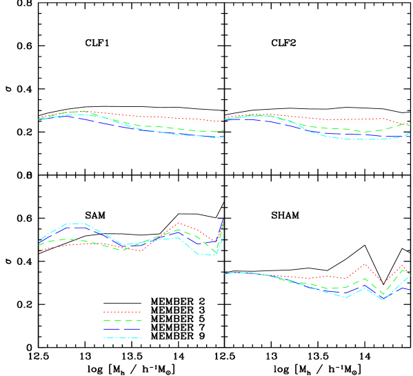
Figure 9.— Similar to the results shown in Fig. 6, but here we only show the $\sigma$ values for four samples: CLF1, CLF2, SAM and SHAM. Lines with different colors represent different member galaxies that are applied to calculate the luminosity gap.

For a given number of members starting from three, we first repeat calculations similar to those shown in Fig. 4, and then split the sample into several bins according to the central galaxy luminosity, starting from $\log L_{c}=9.8$ to $11.0$ with bin width equal to 0.1. The $\Delta\log M_{h}(L_{c},L_{\rm gap})-\log L_{\rm gap}$ relations in the luminosity range $11.0\geq\log L_{c}\geq 9.8$ are used to obtain the best fit parameters that describe the corrections defined in Eq. (11), using the same MCMC algorithm as to the central-second cases. The parameters so obtained are listed in the second to eighth row of Table 2 for cases using the third, fourth, $\cdot\cdot\cdot$, ninth brightest members, respectively. This set of parameters are again only valid for central galaxies within the luminosity range used in fitting. For central galaxies with luminosities outside this region, one can apply the correction factors at $\log L_{c}=9.8$ for faint galaxies and at $\log L_{c}=11.0$ for bright galaxies. We find that the functional form (Eq. 12) describes the overall $\Delta\log M_{h}(L_{c},L_{\rm gap})$ remarkably well for every central galaxy luminosity bins considered, and for all cases regardless which member galaxy used.

Note that the parameters listed in Table 2 are obtained from the CLF1 sample alone. To see if the same correction model can also be applied to other samples, we have checked the $\Delta\log M_{h}$ distributions for the CLF2, SAM and SHAM samples as well, and found that the model also works well.

To show the performance of the correction model, we use the same definition of ‘pre-corrected’ halo mass $\log M^{\prime}_{h}$ as described in Eq. (14). To distinguish with the one obtained from the second brightest member galaxy, we denote it with $\log M^{\prime\prime}_{h}$. As demonstrated in Fig. 5, the scatter is significantly reduced in the $M^{\prime}_{h}(L_{c})$ relation when the second brightest galaxies are used in the halo mass estimate. By using subsequent fainter members, we expect the model to be improved further. In Fig. 8 we compare the ‘pre-corrected’ halo mass as a function of $L_{c}$ between cases using different member galaxies obtained from the CLF1, CLF2, SAM and SHAM samples in different row panels as indicated. The blue open circles with error bars show the median and 68 percentile of $\log M^{\prime}_{h}$, while the solid squares with error bars show the same quantities of $\log M^{\prime\prime}_{h}$.

We see that, in all four samples, involving fainter member galaxies do make further reduction in the scatter of $M_{h}(L_{c})$ relation compared to using the second brightest galaxies. The correction method works more effectively for groups with larger central galaxy luminosity ($\log L_{c}\geq 10.5$). Overall there is about 40% additional reduction in the scatter at the massive end for a fainter (e.g. the fifth - seventh brightest) member galaxy. For lower luminosities ($10.5\geq\log L_{c}\geq 10.0$), the scatter itself shows that including the second or more fainter member galaxies ($\log M^{\prime}_{h}$ v.s. $\log M^{\prime\prime}_{h}$) does not change the scatter significantly, because the halo mass is dominated by the central galaxy itself, and the scatter is already quite small even without the correction.

To better assess the quality of our halo mass estimation with additional member galaxies, we check the difference between the extracted and true halo masses of the groups similar to that shown in the small panels of Fig. 6. We show in Fig. 9 the standard variance, $\sigma$ (Eq. 15), of estimated halo mass from true halo mass of each group. In each panel lines with different colors represent the estimations by using the second, third, fourth $\cdot\cdot\cdot$, ninth brightest members of CLF1, CLF2, SAM and SHAM mock samples, respectively. In general, as expected, using fainter member galaxies does improve the performance of the estimation, especially for massive halos. Interestingly, we also noticed that this improvement is not a monotonically growth with the number of member galaxies we concerned. When the number of member galaxies involved is larger than five, the amounts of improvement actually are quite limited and become negligible when using more than seven members. This feature is caused by the decomposition of our halo mass estimation method: the median $L_{c}-M_{h}$ relation together with a gap dependent correction. This decomposition has the advantage of shrinking the halo mass estimation error only in very poor groups. As we will show in the next section, for groups with more than five members, ‘RANK’ method still performs better given good survey condition. Hence, we treat the seventh member galaxies as the most appropriate option in this paper. In future applications, we will use halo mass estimation by involving seven member galaxies at most.

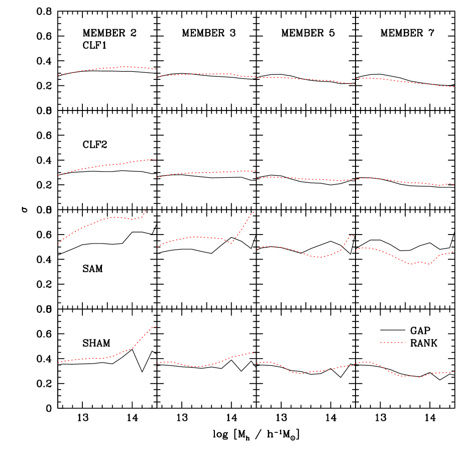
Figure 10.— The comparison of $\sigma$ for two halo mass estimation methods which involve two, three, five and seven brightest member galaxies in each galaxy group of CLF1, CLF2, SAM and SHAM mock samples, respectively. The black solid lines represent the ‘GAP’ method, which are the same as those shown in Fig. 9. Red dotted lines represent the results for the ‘RANK’ method which are described in the §4.1.

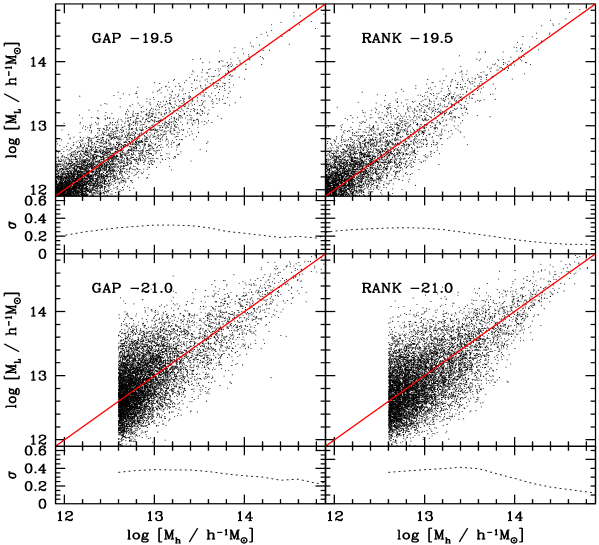
Figure 11.— Similar to Fig. 6, but here the comparisons are carried out between ‘GAP’ and ‘RANK’ methods based on CLF1 mock sample with two different absolute magnitude cuts: $\>{}^{0.1}{\rm M}_{r}-5\log h=-19.5$ (top) and -21.0 (bottom).

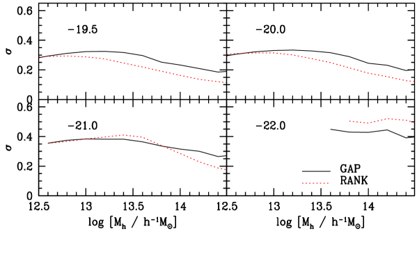
Figure 12.— Similar to Fig. 11, but here only show the $\sigma$ values for both ‘GAP’ (red line) and ‘RANK’ (black line) methods for four absolute magnitude cuts: $\>{}^{0.1}{\rm M}_{r}-5\log h=-19.5$, -20.0, -21.0 and -22.0, respectively.

4. Comparing with the ranking method

Having demonstrated the ability of improving the halo mass estimations using luminosity gap between the central and satellite galaxies, we would like to see if this correction model already achieves the similar good performance of estimating halo mass using the ranking of $L_{G}$ (see Fig. 1). Hereafter we refer these two methods as ‘GAP’ and ‘RANK’, respectively.

4.1. The effect of richness

The results from last section show the performance of ‘GAP’ method somehow depends on how many member galaxies are involved. Meanwhile, this difference of richness certainly will impact on the performance of ‘RANK’ method which is based on the characteristic group luminosity of member galaxies. Therefore, it would be interesting to compare the performances of ‘GAP’ and ‘RANK’ methods on group systems of same richnesses. To make fair comparisons between groups of the same richness, we update the characteristic group luminosity $L_{G}$ with $L^{\prime}_{G}$, which is defined as the total luminosity of the brightest member galaxies to be included. For example, when we only involve three member galaxies, then $L^{\prime}_{G}=L_{1}+L_{2}+L_{3}$. Then, the estimation of halo mass is based on the ranking of $L^{\prime}_{G}$ instead of $L_{G}$.

Fig.10 shows the results of such a comparison. Similar to Fig. 6 and Fig. 9, $\sigma$ is the standard variance of estimated halo masses from true halo masses. In each panel, the solid black line is given by the ‘GAP’ method and is the same as that shown in Fig. 9, which uses the second, third, fifth and seventh brightest members for CLF1, CLF2, SAM and SHAM mock samples, respectively. The dotted red line in each panel is given by the ‘RANK’ method using only two, three, five and seven brightest member galaxies.

In general, the performance of the ‘GAP’ method is somewhat better when only a few (less than five) brightest member galaxies are considered. Then, this advantage is gradually lost when involving more members. In the row only five member galaxies are considered, the performance of ‘GAP’ and corrected ‘RANK’ method is about the same. When the number of member galaxies reach to seven, the ‘RANK’ method tends to be slightly better especially for the SAM sample. Meanwhile, we could also see the impact of including different richness for each galaxy group on ‘RANK’ method is larger than ‘GAP’ method. Thus, ‘GAP’ method would be a better option when only a few galaxy members can be obtained, especially for groups with members less than five.

4.2. The effect of magnitude limit

In real observations, one can only observe galaxies brighter than the survey magnitude limit. This limiting magnitude in-turn allows us to have a complete observation of galaxies of given absolute magnitude to certain redshift. Here we make use of CLF1 mock sample to assess the performances of the ‘RANK’ and ‘GAP’ methods under different absolute magnitude cuts. Note that, for ‘GAP’ method, there are several ways to calculate luminosity gap depending on which member galaxy are used. As we found in previous section that the ‘GAP’ method roughly reaches the best performance at 7th brightest member galaxy, therefore, in what follows, when we refer to ‘GAP’ method, we mean using the maximum available up to 7th member galaxies to estimate the halo masses.

Fig. 11 shows the comparisons between true halo masses directly obtained from the mock samples and the ones estimated using ‘GAP’ (left panels) and ‘RANK’ (right panels) methods, respectively. We chose the absolute magnitude cuts to be $\>{}^{0.1}{\rm M}_{r}-5\log h=-19.5$ (top) and $\>{}^{0.1}{\rm M}_{r}-5\log h=-21.0$ (bottom). Using galaxies brighter than these absolute magnitudes in a group, we estimate the halo masses of the groups according to their characteristic group luminosity and luminosity gap respectively. In general, the performances of ‘RANK’ is slightly better than ‘GAP’ method, especially with a fainter absolute magnitude cut. Once we go to brighter absolute magnitude cut, both the ‘RANK’ and ‘GAP’ methods have worse accuracy of halo mass estimation. The amount of variance between the true halo masses and the estimated ones increase by about 0.1 dex from $\>{}^{0.1}{\rm M}_{r}-5\log h=-19.5$ to $\>{}^{0.1}{\rm M}_{r}-5\log h=-21.0$ for both estimation methods. Nevertheless, we see that the performance of ‘GAP’ method is approaching to that of the ‘RANK’ method. Here, compare to results show in Fig.6, we do see that the systematic deviation in mass estimation disappears.

To reveal in more detail the impact of different magnitude cuts, we plot the comparison of $\sigma$ for both ‘RANK’ and ‘GAP’ estimation methods in Fig.12 to much brighter absolute magnitude cuts: $\>{}^{0.1}{\rm M}_{r}-5\log h=-19.5$, -20.0, -21.0 and -22.0. These absolute magnitude cuts roughly correspond to redshift completeness limit $z=0.09$, 0.103, 0.157, 0.22 in the SDSS observation with apparent magnitude limit $r=17.6$ (e.g. Wang et al. 2007). The black lines in Fig.12 represent the results given by ‘GAP’ method, while red lines are given by ’RANK’ method. Apparently, missing faint member galaxies influences both methods. Compare to ‘GAP’ method, ‘RANK’ method is more sensitive to the increasing of luminosity threshold. In $\>{}^{0.1}{\rm M}_{r}-5\log h=-19.5$ panel, ‘RANK’ method has an obvious advantage over a wide halo mass range, while the situation is inverted at $\>{}^{0.1}{\rm M}_{r}-5\log h=-22.0$. These results may indicate that, for very high redshift or very shallow observations where the luminosity threshold is high, ‘GAP’ method may be a better option. In addition, the ‘GAP’ method is not suffered from the volume calculation which is required in the ‘RANK’ method, thus can be easily implemented to surveys with poor geometry and are flux limited.

5. SUMMARY

Galaxies are thought to form and reside within code dark matter halos. Different galaxy formation processes, e.g., star forming, quenching, AGN feedback, etc., may occur or dominate in halos of different masses. On the other hand, the halos are the building block of the cosmic web, one can use the halo mass functions and clustering properties to understand the nature of our Universe. Within these studies, halo mass estimation from various observations is one of the key challenges. However, such a mission is difficult, especially for poor galaxy systems where only a few brightest member galaxies are observed. Within the galaxy formation framework, the central (brightest) galaxies in the dark matter halos have a rough scaling relation with the masses of the halos: brighter galaxies live in more massive halos. However, the scatter within that scaling relation is very large, especially in massive halos. In this study, we make use of four mock galaxy catalogues, one based on the SAM, one based on the SHAM and the other two on the CLF, to investigate the central-halo scaling relation and to find out a way that can significantly reduce its scatter. Based on these four mock samples, we probed the impact of the luminosity gap, which is defined as the luminosity ratio between the brightest and other member galaxies in the same dark matter halo. In this paper, we take into account a maximum of nine member galaxies in the modeling. We find that the scatter in the central-host halo mass relation is luminosity gap dependent, which in turn can be used to reduce this intrinsic scatter. The main findings of this paper are as follows.

1. We find that the median halo mass for a given central galaxy luminosity can be described by simple relation described by Eq. 10, however with quite large scatter around this median.

2. The scatter in the halo mass depends both on the central galaxy luminosity and the luminosity gap between the central and the subsequent brightest member galaxies.

3. We have obtained a mass correction factor Eq. 12 which is independent to the detailed galaxy formation models, and thus can be applied to any median halo mass - central galaxy luminosity ($M_{h}-L_{c}$) relation to get better estimation of the halo masses.

4. The correction factors can reduce the scatters in halo mass estimations in massive halos by about 50% to 70% depend on which member (second or seventh) galaxies are used.

5. Comparing this ‘GAP’ method with traditional ‘RANK’ method, we find that the former performs better for groups with less than five members, or in observations with very bright magnitude cut. In addition, the ‘GAP’ method does not need to calculate the volume in estimating halo masses, and thus is much easier to be applied to observations with very small volume or with poor geometry.

The above modeling is very useful for our probing of those poor galaxy systems or shallow observations where only a few brightest member galaxies in a halo can be observed. Based on these limited member galaxies, we can have a fairly good estimation of the halo mass, which is important for various astrophysical and cosmological studies.

Appendix A A different definition of luminosity gap

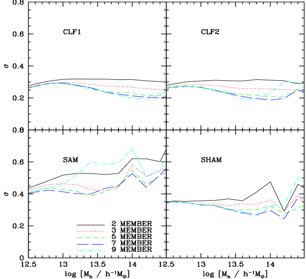
Figure 13.— Similar to the results shown in Fig. 9, but here the $\sigma$ values are given by another definition of luminosity gap for CLF1,CLF2, SAM and SHAM sample respectively. Lines with different colors represent different number of member galaxies that are applied to calculate the luminosity gap.

Throughout the paper, we define the luminosity gap to be the difference between the brightest and the $i$-th brightest member galaxies. In general, we can also define the luminosity gap as the difference between the brightest and all satellite galaxies, $\log L_{\rm gap}=\log L_{c}-\log L_{s}$, here $\log L_{s}$ is defined as the total satellite galaxy luminosity in consideration. For example, if we only consider two brightest member galaxies in a group, $\log L_{s}=L_{2}$. If we choose to include four member galaxies in a group, then $\log L_{s}=L_{2}+L_{3}+L_{4}$, where $L_{3}$ and $L_{4}$ are the luminosities of the third and fourth brightest galaxies in this group.

Then, we applied exactly the same procedure as before using this new luminosity gap definition. First, calculate the $\Delta\log M_{h}(L_{c},L_{\rm gap})-\log L_{\rm gap}$ relations as in Fig. 4 in the luminosity range $10.9\geq\log L_{c}\geq 9.7$. Then, use MCMC algorithm to find the best parameter set which can describe the relation defined by eq. 12 and eq. 3.3. Note that, since we applied total luminosity of member galaxies, the luminosity gap $\log L_{\rm gap}$ can be negative. Overall, the values of $\log L_{\rm gap}$ are roughly in the range $-1.0-2.0$. Using the relation obtained by the new definition of luminosity gap, we estimated the halo mass for each group in four mock samples and compared these estimated halo mass to the true halo mass using $\sigma$ as before. Fig. 13 shows the performance of this new definition of luminosity gap. Compare to those shown in Fig. 9, we can see the tendency and value of $\sigma$ are quite similar in the two figures. In general, the definition for $i$-th member galaxy luminosity is slightly better at massive ends.

References

- Andreon & Hurn (2010) Andreon, S., & Hurn, M. A. 2010, MNRAS, 404, 1922
- Becker et al. (2007) Becker, M. R., McKay, T. A., Koester, B., et al. 2007, ApJ, 669, 905
- Behroozi et al. (2012) Behroozi, P., Wechsler, R., & Wu, H.-Y. 2012, Astrophysics Source Code Library, 1210.008
- Berlind et al. (2006) Berlind, A. A., Frieman, J., Weinberg, D. H., et al. 2006, ApJS, 167, 1
- Biviano et al. (2006) Biviano, A., Murante, G., Borgani, S., et al. 2006, A&A, 456, 23
- Brainerd & Specian (2003) Brainerd, T. G., & Specian, M. A. 2003, ApJ, 593, L7
- Cacciato et al. (2013) Cacciato, M., van den Bosch, F. C., More, S., Mo, H., & Yang, X. 2013, MNRAS, 430, 767
- Cacciato et al. (2009) Cacciato, M., van den Bosch, F. C., More, S., et al. 2009, MNRAS, 394, 929
- Carlberg et al. (1996) Carlberg, R. G., Yee, H. K. C., Ellingson, E., et al. 1996, ApJ, 462, 32
- Carlberg et al. (1997) Carlberg, R. G., Yee, H. K. C., & Ellingson, E. 1997, ApJ, 478, 462
- Collister & Lahav (2005) Collister, A. A., & Lahav, O. 2005, MNRAS, 361, 415
- Conroy et al. (2007) Conroy, C., Prada, F., Newman, J. A., et al. 2007, ApJ, 654, 153
- Cooray et al. (2006) Cooray, Asantha, 2006, MNRAS, 365, 842C
- Crook et al. (2007) Crook, A. C., Huchra, J. P., Martimbeau, N., et al. 2007, ApJ, 655, 790
- Dawson (2013) Dawson, Kyle S.; Schlegel, David J.; Ahn, Christopher P.; et al. 2013, AJ, 145, 10
- Driver et al. (2011) Driver, S. P., Hill, D. T., Kelvin, L. S., et al. 2011, MNRAS, 413, 971
- Eke et al. (2004) Eke, V. R., Baugh, C. M., Cole, S., et al. 2004, MNRAS, 348, 866
- Erickson et al. (1987) Erickson, L. K., Gottesman, S. T., & Hunter, J. H., Jr. 1987, Nature, 325, 779
- Gladders & Yee (2005) Gladders, M. D., & Yee, H. K. C. 2005, ApJS, 157, 1
- Gladders & Yee (2000) Gladders, M. D., & Yee, H. K. C. 2000, AJ, 120, 2148
- Guo (2011) Guo, Qi; White, Simon; et al. 2011, MNRAS, 413, 101
- Guo (2013) Guo, Qi; White, Simon; et al. 2013, MNRAS, 435, 897
- Hao et al. (2010) Hao, J., McKay, T. A., Koester, B. P., et al. 2010, ApJS, 191, 254
- Hearin et al. (2013) Hearin, A. P., Zentner, A. R., Newman, J. A., & Berlind, A. A. 2013a, MNRAS, 430, 1238
- Hearin et al. (2013) Hearin, A. P., Zentner, A. R., Berlind, A. A., & Newman, J. A. 2013b, MNRAS, 433, 659
- Ilbert et al. (2009) Ilbert, O.; Capak, P.; Salvato, M.; Aussel, H.; McCracken, H. J.; Sanders, D. B.; Scoville, N., 2009, ApJ, 690, 1236I
- Jing et al. (1998) Jing, Y. P., Mo, H. J., & Börner, G. 1998, ApJ, 494, 1
- Jones et al. (2009) Jones D. H., et al., 2009, MNRAS, 399, 683
- Kang et al. (2005) Kang, X., Jing, Y. P., Mo, H. J., Borner, G. 2005, ApJ, 631, 21
- Katgert et al. (2004) Katgert, P., Biviano, A., & Mazure, A. 2004, ApJ, 600, 657
- Kim et al. (2002) Kim, R. S. J., Kepner, J. V., Postman, M., et al. 2002, AJ, 123, 20
- Klypin et al. (2011) Klypin, A. A., Trujillo-Gomez, S., & Primack, J. 2011, ApJ, 740, 102
- Koester et al. (2007) Koester, B. P., McKay, T. A., Annis, J., et al. 2007, ApJ, 660, 221
- Li et al. (2012) Li, C., Jing, Y. P., Mao, S., et al. 2012, ApJ, 758, 50
- Liu et al. (2010) Liu, L., Yang, X., Mo, H. J., van den Bosch, F. C., & Springel, V. 2010, ApJ, 712, 734
- Mandelbaum et al. (2013) Mandelbaum, R., Slosar, A., Baldauf, T., et al. 2013, MNRAS, 432, 1544
- McKay et al. (2002) McKay, T. A., Sheldon, E. S., Johnston, D., et al. 2002, ApJ, 571, L85
- Mo et al. (1999) Mo, H. J., Mao, S., & White, S. D. M. 1999, MNRAS, 304, 175
- More et al. (2009a) More, S., van den Bosch, F. C., Cacciato, M., et al. 2009a, MNRAS, 392, 801
- More et al. (2009b) More, S., van den Bosch, F. C., & Cacciato, M. 2009b, MNRAS, 392, 91
- More et al. (2011) More, S., van den Bosch, F. C., Cacciato, M., et al. 2011, MNRAS, 410, 210
- More (2012) More, S. 2012, ApJ, 761, 127
- More et al. (2013) More, S., van den Bosch, F. C., Cacciato, M., et al. 2013, MNRAS, 430, 747
- Norberg et al. (2008) Norberg, P., Frenk, C. S., & Cole, S. 2008, MNRAS, 383, 646
- Nurmi et al. (2013) Nurmi, P., Heinämäki, P., Sepp, T., et al. 2013, MNRAS, 436, 380
- Peacock et al. (2000) Peacock, J.A. & Smith, R. E., 2000, MNRAS, 318, 1144P
- Planck Collaboration et al. (2013) Planck Collaboration, Ade, P. A. R., Aghanim, N., et al. 2013, arXiv:1303.5076
- Prada et al. (2003) Prada, F., Vitvitska, M., Klypin, A., et al. 2003, ApJ, 598, 260
- Robotham et al. (2006) Robotham, A., Wallace, C., Phillipps, S., & De Propris, R. 2006, ApJ, 652, 1077
- Robotham et al. (2011) Robotham, A. S. G., Norberg, P., Driver, S. P., et al. 2011, MNRAS, 416, 2640
- Shen et al. (2014) Shen, S., Yang, X., Mo, H., van den Bosch, F., & More, S. 2014, ApJ, 782, 23
- Springel et al. (2005) Springel, V., White, S. D. M., Jenkins, A., et al. 2005, Nature, 435, 629
- Tago et al. (2010) Tago, E., Saar, E., Tempel, E., et al. 2010, A&A, 514, AA102
- Vale & Ostriker (2004) Vale, A., & Ostriker, J. P. 2004, MNRAS, 353, 189
- Vale & Ostriker (2006) Vale, A., & Ostriker, J. P. 2006, MNRAS, 371, 1173
- van den Bosch et al. (2003) van den Bosch, F. C., Yang, X., & Mo, H. J. 2003, MNRAS, 340, 771
- van den Bosch et al. (2004) van den Bosch, F. C., Norberg, P., Mo, H. J., & Yang, X. 2004, MNRAS, 352, 1302
- van den Bosch et al. (2005) van den Bosch, F. C., Weinmann, S. M., Yang, X., et al. 2005, MNRAS, 361, 1203
- van den Bosch et al. (2005) van den Bosch, F. C., Tormen, G., & Giocoli, C. 2005, MNRAS, 359, 1029
- van den Bosch et al. (2007) van den Bosch, F. C., Yang, X., Mo, H. J., et al. 2007, MNRAS, 376, 841
- van den Bosch et al. (2013) van den Bosch, F. C., More, S., Cacciato, M., Mo, H., & Yang, X. 2013, MNRAS, 430, 725
- Wang et al. (2007) Wang Y., Yang X. Mo H.J., van den Bosch F.C., 2007, ApJ, 664, 608
- Weinmann et al. (2006) Weinmann, S. M., van den Bosch, F. C., Yang, X., et al. 2006b, MNRAS, 372, 1161
- Weinmann et al. (2006) Weinmann, S. M., van den Bosch, F. C., Yang, X., & Mo, H. J. 2006a, MNRAS, 366, 2
- White et al. (2010) White, M., Cohn, J. D., & Smit, R. 2010, MNRAS, 408, 1818
- Willmer et al. (2006) Willmer, C. N. A.; Faber, S. M.; Koo, D. C.; Weiner, B. J.; Newman, J. A.; Coil, A. L.; Connolly, A. J.; Conroy, C.; 2006, ApJ, 647, 853W
- Yan et al. (2003) Yan, R., Madgwick, D. S., & White, M. 2003, ApJ, 598, 848
- Yang et al. (2003) Yang, X., Mo, H. J., van den Bosch, F. C., 2003, MNRAS, 339, 1057Y
- Yang et al. (2004) Yang, X., Mo, H. J., Jing, Y. P., van den Bosch, F. C., & Chu, Y. 2004, MNRAS, 350, 1153
- Yang et al. (2005) Yang, X., Mo, H. J., van den Bosch, F. C., & Jing, Y. P. 2005a, MNRAS, 356, 1293
- Yang et al. (2005) Yang, X., Mo, H. J., Jing, Y. P., & van den Bosch, F. C. 2005c, MNRAS, 358, 217
- Yang et al. (2005) Yang, X., Mo, H. J., van den Bosch, F. C., et al. 2005d, MNRAS, 362, 711
- Yang et al. (2006) Yang, X., Mo, H. J., & van den Bosch, F. C. 2006, ApJ, 638, L55
- Yang et al. (2007) Yang, X., Mo, H. J., van den Bosch, F. C., et al. 2007, ApJ, 671, 153
- Yang et al. (2008) Yang, X., Mo, H. J., & van den Bosch, F. C. 2008, ApJ, 676, 248
- Zandivarez et al. (2006) Zandivarez, A., Martínez, H. J., & Merchán, M. E. 2006, ApJ, 650, 137
- Zaritsky et al. (1993) Zaritsky, D., Smith, R., Frenk, C., & White, S. D. M. 1993, ApJ, 405, 464
- Zheng et al. (2007) Zheng, Zheng; Coil, Alison L.; Zehavi, Idit , 2007, ApJ, 667, 760Z