X-ray Insights into the Nature of PHL 1811 Analogs and Weak Emission-Line Quasars: Unification with a Geometrically Thick Accretion Disk?

Abstract

We present an X-ray and multiwavelength study of 33 weak emission-line quasars (WLQs) and 18 quasars that are analogs of the extreme WLQ, PHL 1811, at $z\approx 0.5$–2.9. New Chandra 1.5–9.5 ks exploratory observations were obtained for 32 objects while the others have archival X-ray observations. Significant fractions of these luminous type 1 quasars are distinctly X-ray weak compared to typical quasars, including 16 (48%) of the WLQs and 17 (94%) of the PHL 1811 analogs with average X-ray weakness factors of 17 and 39, respectively. We measure a relatively hard ($\Gamma=1.16_{-0.32}^{+0.37}$) effective power-law photon index for a stack of the X-ray weak subsample, suggesting X-ray absorption, and spectral analysis of one PHL 1811 analog, J1521+5202, also indicates significant intrinsic X-ray absorption. We compare composite SDSS spectra for the X-ray weak and X-ray normal populations and find several optical–UV tracers of X-ray weakness; e.g., Fe ii rest-frame equivalent width and relative color. We describe how orientation effects under our previously proposed “shielding-gas” scenario can likely unify the X-ray weak and X-ray normal populations. We suggest that the shielding gas may naturally be understood as a geometrically thick inner accretion disk that shields the broad line region from the ionizing continuum. If WLQs and PHL 1811 analogs have very high Eddington ratios, the inner disk could be significantly puffed up (e.g., a slim disk). Shielding of the broad emission-line region by a geometrically thick disk may have a significant role in setting the broad distributions of C iv rest-frame equivalent width and blueshift for quasars more generally.

1. INTRODUCTION

Luminous X-ray emission is considered a universal property of active galactic nuclei (AGNs), and built upon this idea are extragalactic X-ray surveys for finding AGNs efficiently throughout the universe (e.g., Brandt & Alexander, 2015, and references therein). For AGNs that are not radio loud (with a jet-linked X-ray enhancement) or X-ray absorbed, the X-ray-to-optical power-law slope parameter ($\alpha_{\rm OX}$) has a highly significant correlation with 2500 Å monochromatic luminosity ($L_{\rm 2500~{}{\textup{\AA}}}$) across $\approx 5$ orders of magnitude in UV luminosity (e.g., Steffen et al., 2006; Just et al., 2007; Lusso et al., 2010). X-ray emission from AGNs is believed to originate from the accretion-disk “corona” via Comptonization of disk optical/UV/EUV photons (e.g., Turner & Miller, 2009, and references therein), although the details of this mechanism remain mysterious.

Few AGNs are found to be intrinsically X-ray weak, i.e., producing much less X-ray emission than expected from the $\alpha_{\rm OX}$–$L_{\rm 2500~{}{\textup{\AA}}}$ relation (e.g., Gibson et al., 2008). A few candidates have been suggested recently based on Nuclear Spectroscopic Telescope Array (NuSTAR; Harrison et al. 2013) observations of significantly X-ray weak broad absorption line (BAL) quasars (Luo et al., 2013, 2014; Teng et al., 2014). The best-studied intrinsically X-ray weak AGN is the type 1 quasar PHL 1811, a very bright ($B=13.9$) radio-quiet quasar at $z=0.19$ (e.g., Leighly et al., 2007a, b). It is X-ray weak by a factor of $\approx 30$–100 relative to expectations from the $\alpha_{\rm OX}$–$L_{\rm 2500~{}{\textup{\AA}}}$ relation, and its X-ray weakness is likely intrinsic instead of being due to absorption given its canonical X-ray spectrum (power-law photon index $\Gamma=2.3\pm 0.1$), lack of detectable photoelectric X-ray absorption, and short timescale X-ray variability (Leighly et al., 2007b). Interestingly, PHL 1811 also has an unusual UV spectrum (Leighly et al., 2007a), which is dominated by strong Fe ii and Fe iii emission with very weak high-ionization lines. The rest-frame equivalent width (REW) of the C iv $\lambda 1549$ line (6.6 Å) is a factor of $\approx 5$ times smaller than that measured from quasar composite spectra (30 Å); this line is also blueshifted (by $\approx 1400$ km s^-1) and asymmetric, indicative of a wind component in the broad emission-line region (BELR; e.g., Richards et al., 2011). Based on photoionization modeling, Leighly et al. (2007a) suggested that many of the unusual emission-line properties of PHL 1811 are a result of the soft optical-to-X-ray ionizing continuum caused by the intrinsic X-ray weakness.

The intriguing possible connection between the extreme emission-line and X-ray properties of PHL 1811 prompted a search for more such X-ray weak quasars using UV emission-line selection criteria (Wu et al. 2011, hereafter W11). A pilot sample of eight type 1, radio-quiet, non-BAL quasars with PHL 1811-like emission-line properties (including small C iv REWs, large C iv blueshifts, and strong Fe ii and Fe iii emission), termed PHL 1811 analogs, were selected for X-ray study. All of them turned out to be X-ray weak, by factors of $>4.8$ to $\geq 34.5$, confirming the empirical link between the X-ray weakness and unusual UV emission-line properties. However, an X-ray stacking analysis revealed a hard spectrum on average for this sample, albeit with a large uncertainty, suggesting that unlike PHL 1811 itself that appears to be intrinsically X-ray weak, these PHL 1811 analogs may often be X-ray absorbed. More PHL 1811 analogs selected in addition to the eight W11 pilot objects are clearly required to constrain better the nature of these extreme quasars.

There is another small population of type 1 quasars that have X-ray and UV emission-line properties overlapping with those of the PHL 1811 analogs: radio-quiet weak emission-line quasars (WLQs). Strong broad emission lines in the optical and UV are a characteristic feature of radio-quiet quasars. It was thus surprising when McDowell et al. (1995) discovered the first WLQ PG 1407+265, with unusually weak Ly$\alpha$, C iv $\lambda 1549$, C iii] $\lambda 1909$, and H$\beta$ lines. With the large spectroscopic quasar sample provided by the Sloan Digital Sky Survey (SDSS; York et al. 2000), more WLQs were discovered. These were originally at $z>2.2$ where Ly$\alpha$ coverage is available ($\approx 90$ WLQs; e.g., Fan et al., 1999; Anderson et al., 2001; Plotkin et al., 2008, 2010b; Diamond-Stanic et al., 2009), and later extended to lower redshifts ($\approx 100$ WLQs; e.g., Collinge et al., 2005; Hryniewicz et al., 2010; Plotkin et al., 2010a, b; Nikołajuk & Walter, 2012; Meusinger & Balafkan, 2014) requiring weak C iv and/or other lines at longer wavelengths. The fraction of X-ray weak quasars among either the high-redshift or lower-redshift WLQs is high ($\approx 50\%$; Shemmer et al. 2009; Wu et al. 2012, hereafter W12), again suggesting a link between the weak UV line emission and X-ray weakness.

Based on the overall similarities between the PHL 1811 analogs and X-ray weak WLQs, W11 argued that PHL 1811 analogs are a subset of WLQs, despite small technical differences in their UV line REW selection criteria. WLQs contain both X-ray normal and X-ray weak quasars (we adopt an X-ray weakness factor of 3.3 as the dividing threshold between X-ray weak and X-ray normal quasars; see Section 4.1 below), while PHL 1811 analogs are likely X-ray weak WLQs due to the additional selection criteria of strong UV Fe emission and large C iv blueshift (W11; W12). A larger sample of PHL 1811 analogs than the pilot sample of eight would help examine further the above suggested connection.

Except for the unusual UV emission-line and X-ray properties, the PHL 1811 analogs and WLQs appear to be typical quasars in terms of other observable multiwavelength properties (e.g., Lane et al. 2011; W11; W12). Various explanations have been proposed for the nature of the PHL 1811 analogs and WLQs, such as an anemic BELR where there is a significant deficit of line-emitting gas in the BELR (e.g., Shemmer et al., 2010), a brief evolutionary stage where the BELR is not fully developed (e.g., Hryniewicz et al., 2010), a soft ionizing spectral energy distribution (SED) produced by the cold accretion disk of a very massive black hole (e.g., Laor & Davis, 2011), a soft ionizing continuum due to intrinsic X-ray weakness (e.g., Leighly et al., 2007a), and a soft ionizing continuum due to small-scale absorption (e.g., W11; W12). However, for the general population of PHL 1811 analogs and WLQs, the absorption-induced soft ionizing continuum appears the most likely scenario, based on systematic studies, albeit using small samples, of their X-ray and multiwavelength properties (e.g., W11; W12).

A small-scale “shielding gas” scenario was proposed in W11 to explain and unify PHL 1811 analogs and WLQs, which was broadly motivated by the shielding gas generally required in the disk-wind model for BAL quasars (e.g., Murray et al., 1995; Proga et al., 2000). In the W11 scenario, some shielding gas interior to the BELR shields all or most of the BELR from the nuclear ionizing continuum, resulting in the observed weak UV emission lines. If our line of sight intersects the X-ray absorbing shielding gas, a PHL 1811 analog or an X-ray weak WLQ is observed; if not, an X-ray normal WLQ is observed. Since BAL quasars were excluded in the selection of PHL 1811 analogs and WLQs, the inclination angle (with respect to disk normal) should probably still be relatively small so that the line of sight does not intercept the (often equatorial) disk wind which would produce BALs in the observed spectra. The reason this shielding gas is unusually effective at screening the BELR in the PHL 1811 analogs and WLQs remains uncertain, but it should be a rare occurrence given the small numbers of PHL 1811 analogs and WLQs discovered.

The fractions of PHL 1811 analogs and WLQs among typical quasars are small, $\lesssim 1\textrm{--}2\%$ (W11). However, studies of rare and extreme objects often clearly reveal phenomena that are more generally applicable, as such effects are more difficult to identify in the overall population (cf. Eddington, 1922). We shall indeed argue the case for such generality later in this paper (see Section 6.3 below). With the pilot studies of W11 and W12 examining systematically the X-ray and emission-line properties of PHL 1811 analogs and WLQs, progress has been made toward understanding the nature of these extreme quasars (e.g., the W11 shielding-gas scenario). However, the small X-ray sample available in their work, with only eight PHL 1811 analogs and 11 radio-quiet WLQs (which are also divided into X-ray weak and X-ray normal categories for the case of WLQs), limited further investigations. A larger sample is critically needed to reduce the uncertainties of stacking and joint spectral analyses, examine correlations between the degree of X-ray weakness and emission-line properties, assess why PHL 1811 analogs are preferentially X-ray weak, and further explore the shielding-gas scenario.

As an extension of the W11 and W12 work, we present here an X-ray and multiwavelength study of 18 PHL 1811 analogs and 33 WLQs, including 33 objects with new Chandra observations. We describe the sample selection and Chandra data analysis in Sections 2 and 3, respectively. The multiwavelength properties, including the $\alpha_{\rm OX}$ parameters, continuum SEDs, and radio properties, are presented in Section 4. In Section 5, we perform X-ray stacking and joint spectral analyses, estimate Eddington ratios, construct composite SDSS spectra, and identify spectral indicators for the X-ray weak subsample. In Section 6, we discuss the unification of the X-ray weak and X-ray normal PHL 1811 analogs and WLQs under the W11 shielding-gas scenario, and we propose that a geometrically thick inner accretion disk may act as the shielding gas in the general population of PHL 1811 analogs and WLQs. We summarize in Section 7.

We caution that, consistent with the exploratory nature of this work, the PHL 1811 analogs and WLQs could be a heterogeneous population. The discussions and conclusions are mainly applicable to the general population of PHL 1811 analogs and WLQs, and we acknowledge that other explanations are possible for a fraction of our sample. We also stress that PHL 1811 analogs were selected based on their PHL 1811-like UV emission-line properties, and they are not necessarily intrinsically X-ray weak like PHL 1811 itself. In fact, the X-ray weakness of PHL 1811 analogs is likely caused by absorption, based on the studies of W11 and our work here. Throughout this paper, we use J2000 coordinates and a cosmology with $H_{0}=65.1$ km s^-1 Mpc^-1, $\Omega_{\rm M}=0.329$, and $\Omega_{\Lambda}=0.671$ (e.g., Ade et al., 2015). Full J2000 names of the targets are listed in the tables while abbreviated names are used in the text. We quote uncertainties at a 1$\sigma$ confidence level and upper and lower limits at a 90% confidence level.

2. SAMPLE SELECTION AND CHANDRA OBSERVATIONS

2.1. New X-ray Sample of PHL 1811 Analogs

Our new sample of PHL 1811 analogs was selected from the SDSS Data Release 7 (DR7; Abazajian et al. 2009) quasar catalog (Schneider et al., 2010) following similar procedures to those in W11, with the major difference being a relaxation in the redshift requirement. Specifically, we require redshift $z>1.7$, SDSS $r$-band magnitude $m_{r}<18.85$, C iv $\lambda 1549$ REW $<10$ Å, C iv blueshift $>1000$ km s^-1, strong UV Fe iii (UV48 $\lambda 2080$) and/or Fe ii (2250–2650 Å) emission, no detection of BALs or mini-BALs (absorption troughs 500–2000 km s^-1 wide), and radio-loudness parameter $R<10$ (radio quiet). The relaxed redshift requirement allows selection of a larger sample than in W11 which includes more optically bright objects for efficient Chandra observations. The choice of a radio-quiet sample is to avoid any contamination from jet-linked X-ray emission that might confuse the results. Some basic quasar properties (e.g., redshift, C iv REW) were initially adopted or derived from the catalogs of Hewett & Wild (2010) and Shen et al. (2011). The C iv blueshifts were measured based on the adopted redshifts. We later performed our own measurements of the redshifts, emission-line properties (Section 2.3 below), and radio-loudness parameters (Section 4.3 below) for our Chandra targets. The UV Fe ii and Fe iii line strength was assessed visually among an initially selected sample satisfying the other criteria, and quasars with stronger Fe ii and Fe iii emission (relative to the other weak-lined quasars) were favored.

Compared to the redshift requirement in W11, $2.125\leq z\leq 2.385$, our $z>1.7$ criterion no longer requires coverage of the Ly$\alpha$ and UV Fe ii emission, although the visual inspection stage of the Fe ii line strength generally selected targets with $z<3$. An initial sample of 66 quasars was selected, including six of the eight radio-quiet PHL 1811 analogs in W11 (the other two have smaller C iv blueshifts than our criterion here). We ranked these objects according to the REW and blueshift of the C iv line, and selected 10 bright ($m_{r}<18.2$) targets with the lowest C iv REWs and highest C iv blueshifts for Chandra observations. The selected quasars span a redshift range of 1.7–2.9. They were observed in Chandra Cycle 14 with 3.7–9.5 ks exposures (Table 1) using the S3 CCD of the Advanced CCD Imaging Spectrometer (ACIS; Garmire et al. 2003).

In addition, we obtained a 40 ks Chandra exposure of J1521+5202 that had a previous 4 ks Chandra exposure (Just et al., 2007) and was studied as a PHL 1811 analog in W11. This remarkable source is one of the most luminous quasars in the SDSS catalog ($M_{i}=-30.2$; e.g., Just et al., 2007), and we aimed to acquire reliable basic spectroscopic information with this longer Chandra observation. X-ray properties derived from this longer observation are used in the relevant analyses of this study.

2.2. New X-ray Sample of WLQs

Our WLQ targets were mainly selected from the Plotkin et al. (2010b) catalog of radio-quiet WLQs which have REW $\lesssim 5$ Å for all emission features. There was no C iv blueshift requirement for the Plotkin et al. (2010b) WLQs. We chose bright ($i$-band magnitude $m_{i}<18.6$) WLQs, excluding objects that are identified as stars based on their proper motions, have potential absorption features (e.g., intervening absorption, mini-BALs, extremely red continuum), or have already been studied in W11 or Shemmer et al. (2009). There were 21 such WLQs selected from the Plotkin et al. (2010b) catalog. In addition, we include in our WLQ sample two bright radio-quiet quasars found in the literature that have similarly weak emission-line features, HE 0141$-$3932 (Reimers et al. 2005; REW $\lesssim 15$ Å for C iv and Mg ii $\lambda 2799$) and 2QZ J2154$-$3056 (Londish et al. 2004; weak [O iii] $\lambda 5007$ and H$\beta$ emission). These 23 WLQs span a redshift range of 0.5–2.5, and they were observed in Chandra Cycle 14 with 1.5–3.5 ks exposures using the ACIS-S3 CCD (Table 1).

However, of these 23 WLQ targets, J1332+0347 was later found to show a C iv BAL in its VLT/X-shooter spectrum (Plotkin et al. 2015). It is also a lensed quasar (Morokuma et al., 2007) which may have its emission-line REWs affected by gravitational lensing amplification (e.g., Shemmer et al., 2009). Therefore, we will not include J1332+0347 in the figures or our analyses below, since it may not be a bona-fide WLQ. However, we do present the basic properties of this object in Tables 1–3 for completeness.

We also note that HE 0141$-$3932 and 2QZ J2154$-$3056 were selected differently from the other WLQs. However, the inclusion of these two objects does not bias our results, as they do not have SDSS spectra and are not included in the majority of the statistical analyses below. Our final new X-ray sample of WLQs includes 22 objects.

2.3. Redshift, UV Emission-Line, and Continuum Measurements

We measured redshifts and UV emission-line properties for our new X-ray samples of PHL 1811 analogs and WLQs the same way as in Section 2.2 of W11. Briefly, the SDSS Catalog Archive Server (CAS) redshifts were initially adopted. These redshifts may not be precise in some cases due to the weakness and sometimes significant blueshifts of the emission lines. We examined the spectra and made small adjustments for some sources based on strong line features (e.g., Mg ii emission, narrow absorption features). We adopted $z=2.238$ for J1521+5202 based on its best-fit H$\beta$ line (W11). The emission-line properties, including the REWs of the C iv $\lambda 1549$, Si iv $\lambda 1397$, $\lambda 1900$ complex (mainly C iii] $\lambda 1909$), Fe iii UV48 $\lambda 2080$, and Mg ii $\lambda 2799$ emission features, and the blueshift and FWHM of the C iv line, were measured interactively. The wavelength region for each line was chosen based on the upper and lower wavelength limits given in Table 2 of Vanden Berk et al. (2001), and a power-law local continuum was fitted between the lower and upper 10% of the wavelength region for the line measurements.

In addition, we measured the UV Fe ii REW that was not included in the previous studies of W11 and W12; it was measured between 2250 Å and 2650 Å following the same approach above. For three objects that do not have full spectral coverage of this wavelength range, a lower limit was derived; for the two cases where the covered fraction of this line feature is $>60\%$ based on the SDSS quasar composite spectrum (Vanden Berk et al., 2001), an estimated Fe ii REW was also derived from this fractional coverage. The uncertainty of this UV Fe ii REW is dominated by the continuum fitting, and a 10% error is assumed.

The adopted redshifts are listed in Table 1, and the UV emission-line properties are shown in Table 2. We also derived relative SDSS $g-i$ colors, $\Delta(g-i)$, for our targets, which are defined as the colors referenced to the median color at a given redshift (e.g., Richards et al., 2001). The $g-i$ colors were taken from Schneider et al. (2010), and the median color was computed within a redshift bin of $\Delta z=0.1$. The relative $g-i$ colors are listed in Table 3, with positive values representing relatively red spectra. We plot the individual SDSS spectra for the PHL 1811 analogs and WLQs in Figure 1, with the composite spectrum of SDSS quasars from Vanden Berk et al. (2001) and the Hubble Space Telescope (HST) spectrum of PHL 1811 (Leighly et al., 2007a) shown for comparison.

Figure 1.— SDSS spectra for the PHL 1811 analogs and WLQs in the Chandra Cycle 14 sample, following the order in Table 1 (an extended version of this figure showing all the spectra is available in the online journal). The $y$-axis is the flux density in arbitrary linear units. Each spectrum has been corrected for Galactic extinction and smoothed using a boxcar of width 20 pixels, We do not show the spectrum of J1521+5202, which was already included in W11. The composite spectrum of SDSS quasars from Vanden Berk et al. (2001) and the HST spectrum of PHL 1811 (Leighly et al., 2007a) are shown for comparison.

2.4. Previous Samples Used in this Study

In order to improve the statistics of our study, we also include previous samples of radio-quiet PHL 1811 analogs and WLQs from W11 and W12. The basic X-ray and multiwavelength properties of these objects were adopted from W11 and W12. There are also X-ray samples of high-redshift ($z\approx 3$–6) WLQs studied previously (e.g., Shemmer et al., 2006, 2009). We do not include those WLQs here due to the significant difference in redshift (and subsequently different rest-frame SDSS spectral coverage). The general comparison between the high-redshift WLQs and lower-redshift WLQs was presented in Section 5 of W12, and their overall properties are consistent with each other.

We include 7 additional radio-quiet PHL 1811 analogs from W11 (the other radio-quiet PHL 1811 analog in W11 is J1521+5202; see Section 2.1) and 10 radio-quiet WLQs from W12. There is one object, J0903+0708, in W11 that does not satisfy the criteria for being a PHL 1811 analog but should be considered a WLQ. For simplicity of the presentation in this paper, we added this object to the W12 WLQ sample.

2.5. The Full Sample and Its Luminosity, Redshift, and Emission-Line Properties

In the full sample, we have in total 18 ($11+7$) radio-quiet PHL 1811 analogs and 33 ($22+10+1$) radio-quiet WLQs. We show in Figure 2 the locations of these objects in the redshift vs. absolute $i$-band magnitude plane, which highlights the broader redshift range and brighter optical fluxes of the PHL 1811 analogs in our Chandra Cycle 14 sample. There is relatively little overlap between PHL 1811 analogs and WLQs in this plot, purely due to the differing selection approaches (Sections 2.1 and 2.2); physically, they are likely similar types of object (W11).

In Figure 3a we compare the C iv REWs and blueshifts of our sample objects (not all the sources in the full sample have C iv coverage) to those of typical radio-quiet quasars (Richards et al., 2011). The PHL 1811 analogs and WLQs have remarkably weak and strongly blueshifted C iv emission, although C iv blueshift was not a selection criterion for the WLQs. For comparison, only $0.48\%$ of the radio-quiet quasars in Richards et al. (2011) have C iv ${\rm REW}<10$ Å, and $30\%$ ($1.6\%$) have C iv blueshift $>1000$ km s^-1 ($>2000$ km s^-1). Due to the differing selection approaches (e.g., Footnote 4), the PHL 1811 analogs have in general somewhat larger C iv REWs than the WLQs, but we do not believe this indicates any fundamental difference between them; both groups have strikingly weak C iv emission relative to the general quasar population. In Figure 3b we compare the Fe ii REWs for the PHL 1811 analogs and WLQs. By our sample selection, the PHL 1811 analogs also have generally larger Fe ii REWs than the WLQs, although there is significant overlap between the two groups.

Since some of our WLQs are at relatively low redshifts ($z\leq 1.5$) with no C iv coverage in the SDSS spectra, the full sample might have contamination from objects having stronger C iv lines (e.g., Plotkin et al. 2015) or C iv BALs (e.g., similar to J1332+0347 noted above). Therefore, in some of the following analyses, we present results based on the subsample of objects at $z>1.5$ with C iv coverage (the C iv subsample) to avoid such contamination. All the 18 PHL 1811 analogs are in the C iv subsample, and 18 of the 33 WLQs (11 of the 22 in the newly observed X-ray sample of WLQs) are in this subsample.

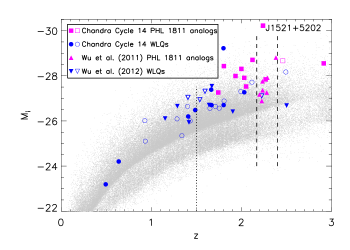
Figure 2.— Redshift vs. absolute $i$-band magnitude for the samples of PHL 1811 analogs and WLQs. The underlying gray dots represent objects from the SDSS DR7 quasar catalog. The vertical dashed lines illustrate the narrow redshift range for the PHL 1811 analogs in W11; our newly selected PHL 1811 analogs have a broader redshift range and generally higher fluxes than the W11 objects. The vertical dotted line marks the redshift ($z=1.5$) where our sample objects start to have C iv coverage and be included in the C iv subsample. Solid symbols represent X-ray weak objects, while open symbols represent X-ray normal objects.

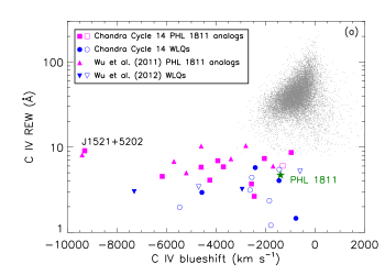
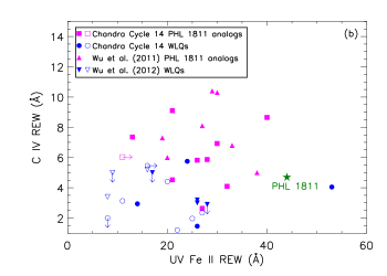
Figure 3.— (a) C iv REW vs. C iv blueshift for the samples of PHL 1811 analogs and WLQs. Only objects having both C iv REW and blueshift measurements are shown here. The underlying gray dots are the 13 582 typical radio-quiet quasars in Richards et al. (2011). The PHL 1811 analogs and WLQs have remarkably weak (as expected from the selection criteria detailed in Sections 2.1 and 2.2) and usually strongly blueshifted C iv emission. (b) C iv REW vs. Fe ii REW for the samples of PHL 1811 analogs and WLQs. Arrows represent upper limits (for C iv REWs) or lower limits (for Fe ii REWs). The PHL 1811 analogs have in general larger Fe ii REWs than the WLQs by selection. In both panels, solid symbols represent X-ray weak objects, while open symbols represent X-ray normal objects; the green star represents PHL 1811.

3. X-RAY DATA ANALYSIS

3.1. X-ray Counts and Photometric Properties

We reduced and analyzed the Chandra Cycle 14 data using mainly the Chandra Interactive Analysis of Observations (CIAO) tools. For each source, we reprocessed the data using the chandra_repro script to apply the latest calibration. The background light curve of each observation was inspected and background flares were removed using the deflare script with an iterative 3$\sigma$ clipping algorithm. The cleaned exposure times are listed in Table 1.

For each source, we created images in the 0.5–8 keV (full), 0.5–2 keV (soft), and 2–8 keV (hard) bands from the cleaned event file using the standard ASCA grade set (ASCA grades 0, 2, 3, 4, and 6). We then ran wavdetect (Freeman et al., 2002) on the images to search for X-ray sources with a “$\sqrt{2}$ sequence” of wavelet scales (i.e., 1, 1.414, 2, 2.828, and 4 pixels) and a false-positive probability threshold of 10^-6. If a source is detected in at least one band, we adopt the wavdetect position that is closest to its SDSS position as the X-ray position. Seven of the 11 PHL 1811 analogs are detected, and 15 of the 22 WLQs are detected. The X-ray-to-optical positional offsets for our targets are small, ranging from 0.1″ to 0.9″ with a mean value of $0.43\pm 0.06\arcsec$. We also verified that there is no confusion with the X-ray source identification (e.g., no close pairs). If a source is not detected by wavdetect, the SDSS position is adopted as the X-ray position.

We performed aperture photometry to assess the detection significance and extract source counts in each of the three energy bands. Source counts were extracted using a 2″-radius circular aperture centered on the X-ray position, which corresponds to encircled-energy fractions (EEFs) of 0.939, 0.959, and 0.907 in the full, soft, and hard bands, respectively. Background counts were extracted from an annular region centered on the X-ray position with inner radius 10″ and outer radius 40″. For each source in each band, we computed a binomial no-source probability, $P_{\rm B}$, to assess the significance of the source signal (e.g., Broos et al., 2007; Xue et al., 2011; Luo et al., 2013), which is defined as

$$P_{\rm B}(X\geq S)=\sum_{X=S}^{N}\frac{N!}{X!(N-X)!}p^{X}(1-p)^{N-X}~{}.$$ (1)

In this equation, $S$ is the total number of counts in the source-extraction region; $N=S+B$, where $B$ is the total number of counts in the background extraction region; $p=1/(1+BACKSCAL)$, where $BACKSCAL$ is the ratio of the area of the background region to that of the source region. $P_{\rm B}$ represents the probability of observing the source counts by chance under the assumption that there is no real source at the relevant location. If the $P_{\rm B}$ value in a band is smaller than 0.01 (corresponding to a $\geq 2.6\sigma$ detection), we considered the source detected in this band and calculated the 1$\sigma$ errors on the net counts, which were derived from the 1$\sigma$ errors on the extracted source and background counts (Gehrels, 1986) following the numerical method in Section 1.7.3 of Lyons (1991). We note that this $P_{\rm B}$ threshold is appropriate in our case where the position of interest is precisely specified in advance. If the $P_{\rm B}$ value is larger than 0.01, we considered the source undetected and derived an upper limit on the source counts using the Bayesian approach of Kraft et al. (1991) for a 90% confidence level. In Table 1, we list the source counts and upper limits in the soft and hard bands.

We derived a 0.5–8 keV effective power-law photon index ($\Gamma_{\rm eff}$) for each source from the band ratio between the hard and soft band counts, calibrated using the Portable, Interactive, Multi-Mission Simulator (PIMMS) with the assumption of a power-law spectrum modified with Galactic absorption (Dickey & Lockman, 1990). $\Gamma_{\rm eff}$ represents the real power-law photon index if the underlying spectrum is truly a power law with Galactic absorption. The uncertainties of (or limits on) the band ratios (and subsequently $\Gamma_{\rm eff}$) were derived using the Bayesian code behr (Park et al., 2006). For sources undetected in both the soft and hard bands, $\Gamma_{\rm eff}$ cannot be constrained and a value of 1.9 was adopted for flux or flux density computations later (Section 4.1 below), which is typical for luminous radio-quiet quasars (e.g., Reeves et al., 1997; Just et al., 2007; Scott et al., 2011). The band ratios and $\Gamma_{\rm eff}$ values are listed in Table 1.

3.2. Spectral Analysis of J1521+5202

J1521+5202 is an exceptionally luminous quasar (e.g., Figure 2). However, it is remarkably X-ray weak (by a factor of $\approx 35$), as first reported by Just et al. (2007) using a 4 ks Chandra observation. As a PHL 1811 analog, J1521+5202 was studied in W11, which also presented a near-infrared (NIR) spectrum showing very weak [O iii] emission and a higher optical Fe ii/H$\beta$ ratio than those of typical quasars. The source was only weakly detected in the 4 ks Chandra observation with 3 full-band counts, preventing further constraints on the band ratio and effective photon index. With our much longer Chandra observation (37.1 ks cleaned exposure) of J1521+5202, we derived a band ratio of $1.1_{-0.2}^{+0.3}$ and an effective power-law photon index of $0.6\pm 0.2$ (Table 1). This flat effective photon index, compared to the typical value of $\Gamma\approx 1.9$ for luminous radio-quiet quasars (e.g., Reeves et al., 1997; Just et al., 2007; Scott et al., 2011), suggests that the significant X-ray weakness of this source is likely due to strong absorption.

We then performed basic spectral analysis for J1521+5202. The 0.3–8 keV (rest-frame 1.0–25.5 keV) spectrum was extracted using the CIAO specextract script within a circular aperture of 4″ radius centered on the X-ray position. There are $\approx 90$ source counts extracted including $<1$ background count. The background spectrum was extracted from an annular region with inner radius 6″ and outer radius 15″, which is free of X-ray source contamination. Given the limited source counts, we fitted the spectrum using XSPEC (version 12.8.1; Arnaud 1996) with a simple model consisting of a power law modified by both intrinsic absorption (at $z=2.24$) and Galactic absorption. The $C$ statistic (cstat) was used due to the limited photon counts (Cash, 1979). The best-fit photon index is $\Gamma=1.51_{-0.35}^{+0.38}$, and the intrinsic absorption column density is $N_{\rm H}=(1.31_{-0.48}^{+0.56})\times 10^{23}$ cm^-2 ($C=88$ for 75 degrees of freedom). The spectrum and the best-fit model are displayed in Figure 4. There is a possible emission-line feature at rest-frame 7.5 keV, which would likely correspond to a blueshifted Fe line if confirmed (e.g., Reeves et al., 2004). More data are required to constrain this feature.

The spectral analysis also suggests significant X-ray absorption in J1521+5202, in agreement with the simple flat $\Gamma_{\rm eff}$ argument above. We note that the absorption derived from our simple spectral model cannot entirely account for the observed X-ray weakness; after correction for this absorption J1521+5202 is still a factor of $\approx 7$ times X-ray weak (a $\approx 2.5\sigma$ deviation from the $\alpha_{\rm OX}$–$L_{\rm 2500~{}{\textup{\AA}}}$ relation). This result suggests that our simple model probably did not recover the real (larger) absorption column density associated with a more complex absorber, as is commonly seen in highly obscured AGNs. Alternatively, J1521+5202 may also be intrinsically X-ray weak by a factor of a few besides the strong X-ray absorption.

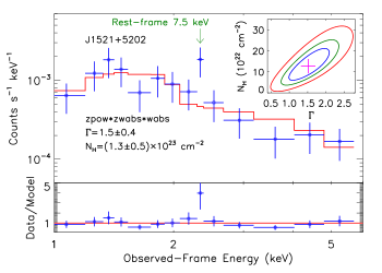
Figure 4.— Chandra spectrum of J1521+5202 (blue) overlaid with the best-fit model (red). The 0.3–8 keV spectrum was fitted with an absorbed power-law model modified with Galactic absorption using cstat in XSPEC. For display purposes, the data are grouped with a minimum of six counts per bin. The inset shows the best-fit $\Gamma$ and $N_{\rm H}$ values (magenta plus), and their 1$\sigma$ (blue), 2$\sigma$ (green), and 3$\sigma$ (red) contours. The bottom panel shows the ratio of the data to the best-fit model. The best-fit model suggests strong intrinsic X-ray absorption, with $N_{\rm H}=(1.3\pm 0.5)\times 10^{23}$ cm^-2.

4. MULTIWAVELENGTH PROPERTIES

4.1. Distribution of the X-ray-to-Optical Power-Law Slopes

We measured the $\alpha_{\rm OX}$ parameters for our Chandra Cycle 14 sample objects. The rest-frame 2500 Å flux densities were adopted from the Shen et al. (2011) SDSS quasar catalog; for three objects that were not included in this catalog, the flux densities were interpolated/extrapolated from their optical photometric data. The rest-frame 2 keV flux densities were derived from the soft-band net counts (Table 1) using PIMMS assuming a power-law spectrum modified with Galactic absorption; the observed soft band (0.5–2 keV) covers rest-frame 2 keV for our sources. If a source is not detected in the soft band, an upper limit on $f_{2~{}{\rm keV}}$ was calculated. There are two sources, J0147+0003 and J1133+1142, that are not detected in the soft band but are detected in the hard band. We still present upper limits on $f_{2~{}{\rm keV}}$ (and $\alpha_{\rm OX}$) for these two sources, although the $f_{2~{}{\rm keV}}$ flux density could be estimated via extrapolation of the hard-band flux assuming a power-law photon index. This approach does not affect the analyses in this study. The $\alpha_{\rm OX}$ values, along with other relevant parameters, are listed in Table 3. The level of X-ray weakness is usually measured by the $\Delta\alpha_{\rm OX}$ parameter, which is defined as the difference between the observed $\alpha_{\rm OX}$ and the one expected from the $\alpha_{\rm OX}$–$L_{\rm 2500~{}{\textup{\AA}}}$ relation ($\Delta\alpha_{\rm OX}=\alpha_{\rm OX,obs}-\alpha_{\rm OX,exp}$). From $\Delta\alpha_{\rm OX}$, we can derive the factor of X-ray weakness ($f_{\rm weak}=403^{-\Delta\alpha_{\rm OX}}$) with respect to the expected X-ray flux. These parameters are also listed in Table 3.

The $\alpha_{\rm OX}$ vs. $L_{\rm 2500~{}{\textup{\AA}}}$ distribution for our full sample is displayed in Figure 5; also shown for comparison are PHL 1811 and some typical AGN samples (Steffen et al., 2006; Just et al., 2007; Gibson et al., 2008). We adopt $\Delta\alpha_{\rm OX}=-0.2$ ($f_{\rm weak}=3.3$) to be the dividing threshold between X-ray weak and X-ray normal quasars, which corresponds to a $\approx 1.3\sigma$ ($\approx 90\%$ single-sided confidence level) offset given the $\alpha_{\rm OX}$ rms scatter in Table 5 of Steffen et al. (2006). A remarkable fraction of our sample sources are X-ray weak, similar to PHL 1811. Specifically, of the 18 PHL 1811 analogs, 17 ($94_{-23}^{+6}\%$) are X-ray weak, and 16 ($48_{-12}^{+15}\%$) of the 33 WLQs are X-ray weak. In the C iv subsample, 8 ($44_{-15}^{+22}\%$) of the 18 WLQs are X-ray weak. For comparison, the fraction of X-ray weak objects in the improved version of Gibson et al. (2008) Sample B (see Footnote 16 of W11) is only 7.6% (10/132).

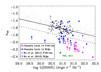
Figure 5.— X-ray-to-optical power-law slope ($\alpha_{\rm OX}$) vs. 2500 Å monochromatic luminosity for the samples of PHL 1811 analogs and WLQs. For comparison, the 132 radio-quiet, non-BAL quasars in the improved version of Gibson et al. (2008) Sample B (see Footnote 16 of W11) are represented by the black dots, and PHL 1811 is shown as the green star. The small grey dots and downward arrows (upper limits) are from the samples of Steffen et al. (2006) and Just et al. (2007), and the solid line represents the Just et al. (2007) $\alpha_{\rm OX}$–$L_{\rm 2500~{}{\textup{\AA}}}$ relation. The dashed line ($\Delta\alpha_{\rm OX}=-0.2$) marks the division between X-ray weak and X-ray normal quasars adopted in this study.

The significantly different fractions of X-ray weak objects among typical quasars and our samples of PHL 1811 analogs and WLQs are also evident in the $\Delta\alpha_{\rm OX}$ distributions (Figure 6). As in W11 and W12, we used the Peto-Prentice test implemented in the Astronomy Survival Analysis package (ASURV; e.g., Feigelson & Nelson 1985; Lavalley et al. 1992) to assess whether two samples follow the same distribution. For PHL 1811 analogs, the probability of their $\Delta\alpha_{\rm OX}$ values being drawn from the same parent population as those of typical quasars (improved version of Gibson et al. 2008 Sample B) is $\approx 10^{-23}$ (10.4$\sigma$). For WLQs, this probability is $3\times 10^{-5}$ (4.1$\sigma$).

Since most of our X-ray weak PHL 1811 analogs and WLQs are not X-ray detected and only upper limits on $\Delta\alpha_{\rm OX}$ are available, we also performed X-ray stacking analyses (see Section 5.1 below) to obtain the average level of X-ray weakness. The stacking results are listed in Table 4 as subsamples “P1811A SB undet” and “WLQ undet” for the undetected sources (excluding two XMM-Newton undetected sources), and the stacked $\Delta\alpha_{\rm OX}$ values are plotted as gray bars in Figure 6. The corresponding average X-ray weakness factors for the undetected PHL 1811 analogs and WLQs are 513 and 108, respectively. As noted above, there are two PHL 1811 analogs in the stacked sample, J0147+0003 and J1133+1142, that are not detected in the soft band but are detected in the hard band. Excluding these two sources from the stacking still yields a large negative stacked $\Delta\alpha_{\rm OX}$ value ($-0.87$), as shown in the results for subsample “P1811A undet” in Table 4.

Including detected objects, the stacked $\Delta\alpha_{\rm OX}$ values are $-0.61$ and $-0.47$ for the X-ray weak PHL 1811 analogs and WLQs, corresponding to average X-ray weakness factors of 39 and 17, respectively. The X-ray weak WLQs in the C iv subsample have a similar stacked $\Delta\alpha_{\rm OX}$ value ($-0.62$; average X-ray weakness factor of $\approx 41$) to the X-ray weak PHL 1811 analogs. In an absorption scenario, an X-ray weakness factor of 40 corresponds to $N_{\rm H}\approx 9\times 10^{23}$ cm^-2 for $z=2$ and $\Gamma=1.9$ in the MYTorus model (Murphy & Yaqoob, 2009). Using the Kaplan–Meier estimator in ASURV, we also derived the mean $\Delta\alpha_{\rm OX}$ values for the X-ray weak PHL 1811 analogs and WLQs, which are $-0.49\pm 0.03$ and $-0.38\pm 0.02$, respectively. Note that the Kaplan–Meier estimator assumes that the censored data have an identical distribution as the measured data (Feigelson & Nelson, 1985), which may not be applicable to our $\Delta\alpha_{\rm OX}$ values here; also, the mean and stacked values differ in the sense that the mean $\Delta\alpha_{\rm OX}$ estimates the geometric mean of the X-ray weakness factors while the stacked $\Delta\alpha_{\rm OX}$ estimates the arithmetic mean.

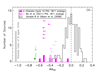
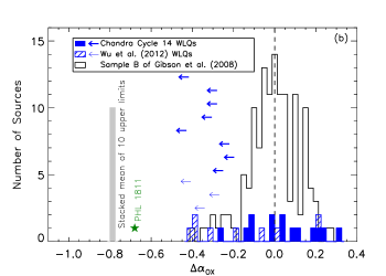
Figure 6.— Distribution of the $\Delta\alpha_{\rm OX}$ values for the (a) PHL 1811 analogs and (b) WLQs in our sample. The solid and hatched shaded histograms (thick and thin leftward arrows) represent X-ray detected (undetected) sources in the Chandra Cycle 14 sample and the previous W11 or W12 sample, respectively. In both panels, the gray bar shows the average $\Delta\alpha_{\rm OX}$ value for the undetected sources estimated via stacking analyses (see Section 5.1 below); there is one XMM-Newton undetected source that was not included in the stacking in each case. For comparison, the $\Delta\alpha_{\rm OX}$ distribution for the 132 Gibson et al. (2008) Sample B quasars is presented as the unshaded histogram, and the $\Delta\alpha_{\rm OX}$ value of PHL 1811 is shown as the green star. A significant fraction of the PHL 1811 analogs and WLQs are X-ray weak compared to typical quasars.

4.2. IR-to-X-ray Spectral Energy Distributions

We constructed infrared (IR) to X-ray continuum SEDs for our full sample of PHL 1811 analogs and WLQs, using photometric data collected from the Wide-field Infrared Survey Explorer (WISE; Wright et al. 2010), Two Micron All Sky Survey (2MASS; Skrutskie et al. 2006), SDSS, and/or Galaxy Evolution Explorer (GALEX; Martin et al. 2005) catalogs. The optical and UV data have been corrected for Galactic extinction following the dereddening approach of Cardelli et al. (1989) and O’Donnell (1994). The combined SEDs for the PHL 1811 analogs and WLQs are displayed in Figures 7 and 8, respectively. The mean SED of optically luminous SDSS quasars from Richards et al. (2006) is shown for comparison. Because of our sample selection criteria, the PHL 1811 analogs are about a factor of $\approx 3$ times more optically luminous on average than the Richards et al. (2006) optically luminous SDSS quasars, while the WLQs have comparable luminosities to the SDSS quasars. Regardless of whether they are X-ray weak or X-ray normal, our PHL 1811 analogs and WLQs in general have IR-to-UV SEDs similar to those of typical quasars. Such SEDs differ significantly from those of BL Lac objects, indicating that our sample is not contaminated by any radio-quiet BL Lac candidates (e.g., see discussion on J1109+3736 in W12). Studies of a sample of high-redshift ($z=2.7$–5.9) WLQs also found typical quasar SEDs (Lane et al., 2011).

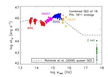
Figure 7.— Combined SED for the PHL 1811 analogs. The IR-to-UV SED data were collected from the WISE (red), 2MASS (magenta), SDSS (blue), and GALEX (orange) catalogs. These data have been corrected for Galactic extinction following the dereddening approach of Cardelli et al. (1989) and O’Donnell (1994). The green data points and arrows show the 2 keV luminosities and upper limits. The SED for each object was scaled to the composite quasar SED of optically luminous quasars (Richards et al., 2006) at rest-frame 3000 Å, and then combined. Some of the GALEX data points affected by the Lyman break are removed in the combined SED for display purposes. The combined IR-to-UV SED of PHL 1811 analogs is similar to the composite quasar SED. We do not separate the X-ray normal PHL 1811 analog (J1537+2716) from the other X-ray weak objects as it also has a typical quasar SED.

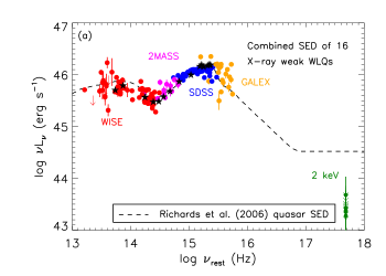
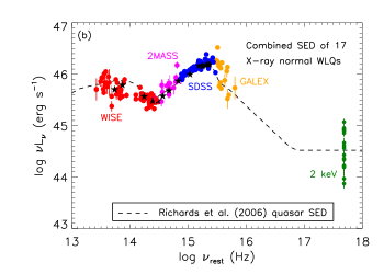
Figure 8.— Same as Figure 7 but for the (a) X-ray weak and (b) X-ray normal WLQs. The black stars represent the composite SED of 18 high-redshift ($z=2.7$–5.9) WLQs in Lane et al. (2011). The combined SEDs of the X-ray weak and X-ray normal WLQs are similar from the IR to UV, and they agree well with the composite quasar SED.

We estimated bolometric luminosities ($L_{\rm Bol}$) for our sample objects by integrating the Richards et al. (2006) composite SED (between $10^{12.5}$–$10^{19}$ Hz) scaled to their rest-frame 3000 Å luminosities. The resulting bolometric luminosities for the full sample are listed in Table 5, ranging from $\approx 2\times 10^{45}$ erg s^-1 to $\approx 2\times 10^{48}$ erg s^-1 with a median value of $\approx 8\times 10^{46}$ erg s^-1. We compared these bolometric luminosities to those estimated via integrating the SEDs directly. The ratios of the two luminosities have a median value of $\approx 1$, and an rms scatter of $\approx 3$, suggesting that the typical uncertainty associated with the estimated $L_{\rm Bol}$ values is approximately a factor of three. There may also be additional systematic uncertainty if the EUV properties of these objects differ from those of typical quasars (e.g., see Sections 6.1 and 6.2; Krawczyk et al. 2013).

4.3. Radio Properties

Only radio-quiet ($R<10$) quasars are included in our sample. The radio-loudness parameter was computed as $R=f_{5~{}{\rm GHz}}/f_{\rm 4400~{}{\textup{\AA}}}$ (e.g., Kellermann et al., 1989), where the rest-frame 5 GHz and 4400 Å flux densities were converted from the observed 1.4 GHz and rest-frame 2500 Å flux densities (or their upper limits) assuming a radio power-law slope of $\alpha_{\rm r}=-0.8$ ($f_{\nu}\propto\nu^{\alpha}$; e.g., Falcke et al. 1996; Barvainis et al. 2005) and an optical power-law slope of $\alpha_{\rm o}=-0.5$ (e.g., Vanden Berk et al. 2001). We obtained radio flux information at 1.4 GHz via cross-matching to the Faint Images of the Radio Sky at Twenty-Centimeters (FIRST) survey catalog (Becker et al., 1995; White et al., 1997). For sources not detected by the FIRST survey, the upper limits on the radio fluxes were set to $0.25+3\sigma_{\rm rms}$ mJy, where $\sigma_{\rm rms}$ is the rms noise of the FIRST survey at the source position and 0.25 mJy is to account for the CLEAN bias (White et al., 1997). The $R$ values for the Chandra Cycle 14 targets are listed in Table 3.

Given the radio-quiet selection criterion, all our sample objects have optical-to-radio power-law slopes $\alpha_{\rm RO}>-0.21$ (e.g., Equation 4 of W12) and are in the radio-quiet region of the $\alpha_{\rm OX}$ vs. $\alpha_{\rm RO}$ plot (Figure 7 of W12). However, the two objects with the highest $R$ values in our sample (J0844+1245 with $R=8.0$ and J1156+1848 with $R=7.4$; see Table 3) are considered radio-intermediate in Shen et al. (2011) with $R_{\rm Shen}=11.2$ and $R_{\rm Shen}=10.6$, respectively. The radio-loudness parameter was defined differently in Shen et al. (2011) with $R_{\rm Shen}=f_{5~{}{\rm GHz}}/f_{\rm 2500~{}{\textup{\AA}}}$, which leads to the above small discrepancy. Both quasars are X-ray normal, and we cannot exclude entirely the effect of jet contamination in these two objects. In fact, J0844+1245 is an outlier in the diagnostic plot for X-ray weak quasars (Figure 16 below), which might be related to its relatively high radio loudness. Since both objects are still radio-quiet under our definition, and we have also verified that the inclusion of the two does not affect our statistical analyses significantly, we do not remove them from our study.

5. SAMPLE ANALYSES

5.1. X-ray Spectral Stacking Analyses of the X-ray Weak Objects

The X-ray spectral analysis of J1521+5202 (Section 3.2) suggested significant X-ray absorption. For the other X-ray weak objects in our sample, there are few X-ray photons detected for spectral analyses. The derived effective photon indices (Table 1) also have large uncertainties and cannot constrain whether a source has a flat X-ray spectrum that is indicative of absorption. In this case, X-ray stacking analyses are often used to assess the average spectral properties of the sample. With this approach, W11 and W12 found relatively flat/hard stacked effective photon indices for their samples, although with large error bars, suggestive of X-ray absorption. With the addition of our new X-ray samples, we can improve the statistics of the stacking results and obtain tighter spectral constraints.

We stacked the X-ray photometry by combining the extracted source and background counts of individual sources and following the same procedure as in Section 3.1 to derive photometric properties of the stacked source. Since our objects are generally at high redshifts (a mean value of $z=1.85$ for the full X-ray weak sample), we are probing the highly penetrating X-ray emission in the $\approx 2$–23 keV rest-frame band that is more reliable for assessing the presence of heavy absorption than lower-energy observations. Stacking analyses were performed for several subsamples of X-ray weak objects; the results are given in Table 4, which include the number of sources used in the stacking, mean redshift, total stacked exposure time, stacked soft- and hard-band counts, stacked effective photon index, and stacked $\alpha_{\rm OX}$ and $\Delta\alpha_{\rm OX}$. For the full X-ray weak sample, the stacked effective photon index is relatively hard ($\Gamma_{\rm eff}=1.37_{-0.23}^{+0.25}$) compared to the typical value of $\Gamma\approx 1.9$ for luminous radio-quiet quasars (e.g., Reeves et al., 1997; Just et al., 2007; Scott et al., 2011). The hard average spectral shape is more evident in the subsample of X-ray weak PHL 1811 analogs, with $\Gamma_{\rm eff}=1.16_{-0.32}^{+0.37}$. The stacking results suggest that, unlike PHL 1811 itself that appears intrinsically X-ray weak (at least in the 0.5–8 keV band), these X-ray weak PHL 1811 analogs and WLQs on average are X-ray absorbed, consistent with the conclusion from the spectral analysis of J1521+5202 in Section 3.2. However, given the uncertainties associated with the stacking procedure (e.g., individual sources contribute differently to the stacked signal due to the different fluxes, exposure times, and rest-frame bands probed), we cannot exclude the possibility that a fraction of the sources are intrinsically X-ray weak like PHL 1811 (e.g., those sources with no or poor constraints on $\Gamma_{\rm eff}$).

5.2. Joint Spectral Fitting of the X-ray Normal Objects

The X-ray stacking analyses of the X-ray weak objects likely did not provide constraints on their intrinsic X-ray spectral shapes (due to the likely modification of their spectra by X-ray absorption), and these objects have too few X-ray photons for spectral fitting (the stacked number of counts for all the X-ray weak objects is only 87). Therefore, to obtain a relatively tight constraint on the intrinsic X-ray power-law photon indices of PHL 1811 analogs and WLQs, we performed joint spectral fitting of the one X-ray normal PHL 1811 analog and 17 X-ray normal WLQs. The individual source and background spectra were extracted following the same procedure as in Section 3.2, and all eighteen spectra in the rest-frame $>2$ keV band were fitted jointly with an absorbed power-law model using cstat in XSPEC, allowing each source to have its own redshift and Galactic column density. There are $\approx 610$ total spectral counts for the fitting including only $\approx 2$ background counts, and these spectral counts are not dominated by the counts from one or a few objects.

The best-fit photon index is $\Gamma=2.18\pm 0.09$ ($C=449$ for 487 degrees of freedom), and no intrinsic absorption is required with an upper limit of $N_{\rm H}<2.9\times 10^{21}$ cm^-2. The 1–3$\sigma$ contours for the best-fit $\Gamma$ and $N_{\rm H}$ values are shown in Figure 9. The same analysis was also performed for the C iv subsample, which includes one X-ray normal PHL 1811 analog and nine X-ray normal WLQs. The resulting photon index is slightly higher, $\Gamma=2.26\pm 0.11$ ($C=283$ for 330 degrees of freedom), and no intrinsic absorption is required ($N_{\rm H}<1.4\times 10^{21}$ cm^-2). Similar joint fitting was performed for seven high-redshift radio-quiet WLQs in Shemmer et al. (2009), and their resulting $\Gamma$ constraint is consistent with our $\Gamma$ values within the errors, although our uncertainties are factors of $\approx 5$ times smaller owing to the substantially larger number of spectral counts available.

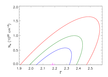
Figure 9.— Contour plot for the photon index and intrinsic absorption column density from the joint spectral analysis for the X-ray normal PHL 1811 analogs and WLQs. The blue, green, and red curves are the 1$\sigma$, 2$\sigma$, 3$\sigma$ contours, respectively. The magenta plus sign indicates the best-fit $\Gamma$ and $N_{\rm H}$ values.

5.3. Eddington-Ratio Estimates

The extreme emission-line properties of PHL 1811 analogs and WLQs could perhaps be related to rapid or even super-Eddington accretion (e.g., Leighly et al. 2007a, b; Shemmer et al. 2010; W11), and thus we estimated their Eddington ratios ($L_{\rm Bol}/L_{\rm Edd}$) based on their estimated bolometric luminosities and supermassive black hole (SMBH) masses. Most of our PHL 1811 analogs and WLQs have their SMBH masses estimated in Shen et al. (2011) using the single-epoch virial mass approach, with 25 objects having Mg ii-based estimates and 21 objects having C iv-based estimates. The C iv virial mass approach is likely not applicable for our objects as the prominent C iv blueshifts indicate a strong wind component for the C iv BELR (e.g., Baskin & Laor, 2005; Richards et al., 2011; Trakhtenbrot & Netzer, 2012; Shen, 2013), and C iv-based masses may be an order of magnitude higher than the real values for quasars with weak C iv lines (e.g., Kratzer & Richards, 2015).

For the 25 objects with Mg ii-based SMBH masses, the median $L_{\rm Bol}/L_{\rm Edd}$ value is 0.27 with an interquartile range of 0.17 to 0.38 (the mean $L_{\rm Bol}/L_{\rm Edd}$ value is 0.39). Even the Mg ii-based SMBH masses are perhaps not reliable for our objects that have weak Mg ii line emission, although not as abnormally weak as the C iv line emission (e.g., Plotkin et al. 2015). A recent VLT/X-shooter study of WLQs (Plotkin et al., 2015) also suggests that, at least sometimes, the Mg ii BELR is complex and may not be virialized in these exceptional objects.

Four of the objects with Mg ii-based masses (J0945+1009, J1411+1402, J1417+0733, and J1447$-$0203) recently have had their masses estimated using the H$\beta$ line profiles (Plotkin et al. 2015), and the masses are on average smaller by a factor of $\approx 3$. The H$\beta$ lines of WLQs are generally weak at a similar level to their Mg ii lines (Plotkin et al. 2015), but the H$\beta$ mass estimator is considered the most reliable one among all the single-epoch virial mass approaches (e.g., Shen, 2013, and references therein). The estimated Eddington ratios for these four objects plus J1521+5202 which also has an H$\beta$-based mass (W11) range from 0.9 to 2.8 with a median value of 1.4 (a mean value of 1.7). The available SMBH mass and Eddington-ratio estimates for our full sample are listed in Table 5. The uncertainties on these SMBH masses include measurement errors ($\approx 0.15$ dex; Shen et al. 2011), systematic errors of the virial-mass approach ($\approx 0.4$–0.5 dex; e.g., Shen 2013), and additional systematic errors (unknown but likely large) related to the likely unusual BELRs of our extreme quasars. Given the substantial uncertainties associated with the SMBH masses and likely also the estimated bolometric luminosities (see Section 4.2), the estimated Eddington ratios do not provide strong constraints on the accretion status of the PHL 1811 analogs and WLQs.

We also make basic estimates of $L_{\rm Bol}/L_{\rm Edd}$ from the hard X-ray power-law photon indices obtained from our joint spectral analyses (Section 5.2), which have been demonstrated to be a useful direct probe of the Eddington ratio (e.g., Shemmer et al., 2008; Risaliti et al., 2009; Brightman et al., 2013). Quasars with high Eddington ratios generally have very soft X-ray photon indices. For example, PHL 1811 has $\Gamma=2.3\pm 0.1$ and $L_{\rm Bol}/L_{\rm Edd}\approx 1.6$ (Leighly et al., 2007b). Based on the empirical $\Gamma\textrm{--}L_{\rm Bol}/L_{\rm Edd}$ relations (Shemmer et al., 2008; Risaliti et al., 2009; Brightman et al., 2013), the best-fit hard X-ray photon index for our X-ray normal objects, $\Gamma\approx 2.2$, corresponds to $L_{\rm Bol}/L_{\rm Edd}\approx 1$. Therefore, the joint spectral fitting results suggest high Eddington ratios for our X-ray normal objects, or our PHL 1811 analogs and WLQs in general considering that the X-ray weak and X-ray normal objects could be unified (W11; see also Section 6 below). There is substantial object-to-object intrinsic scatter in the $\Gamma\textrm{--}L_{\rm Bol}/L_{\rm Edd}$ relations. Thus, by using the average $\Gamma$ from the joint spectral fitting of 10–18 objects, our constraint on the typical $L_{\rm Bol}/L_{\rm Edd}$ should be more reliable than that from the $\Gamma$ values of a few individual objects.

In summary, the Eddington-ratio estimates derived from the virial SMBH masses are highly uncertain and perhaps systematically in error. We caution that individual measurements should not be over-interpreted and, at best, one can look at the group properties for some average indication. The group properties from the H$\beta$-based virial masses suggest the Eddington ratio may be high. Meanwhile, the large hard X-ray photon index from the joint spectral fitting suggests a high Eddington ratio for our objects as a group. We consider it plausible that our PHL 1811 analogs and WLQs are accreting at high or even super-Eddington rates.

5.4. Composite SDSS Spectra

We constructed composite SDSS spectra for our PHL 1811 analogs and WLQs, to compare their average UV spectral properties to those of PHL 1811 and typical quasars and also to make comparisons between the X-ray weak and X-ray normal populations within our sample. Median composite spectra were created following Vanden Berk et al. (2001). Basically, each individual spectrum was corrected for Galactic extinction, smoothed using a boxcar of width 10 pixels, and normalized at rest-frame 2240 Å. The continuum at rest-frame 2240 Å is not significantly contaminated by Fe ii or other lines (e.g., Rafiee & Hall, 2011). The composite spectra were derived by computing the median flux density at each wavelength where at least five objects have spectral coverage.

The composite SDSS spectrum for the 17 X-ray weak PHL 1811 analogs is shown in Figure 10a; the Vanden Berk et al. (2001) composite spectrum of SDSS quasars and the HST spectrum of PHL 1811 (Leighly et al., 2007a) are included for comparison. The weak emission lines, including C iv, C iii], and Mg ii, are evident in PHL 1811 and its analogs. Meanwhile, the PHL 1811 analogs have similar Fe iii UV48 $\lambda 2080$ and UV Fe ii (2250–2650 Å) emission to the SDSS composite spectrum, while PHL 1811 has even stronger UV Fe iii and Fe ii emission. On average, PHL 1811 and its analogs have similar continua that are redder than the SDSS composite spectrum between $\approx 1500$–2700 Å. Using the SDSS filter information and the median redshift of $z=2.2$, we measured a relative $g-i$ color (in the observed frame) of $\Delta(g-i)=0.24$ for the PHL 1811 analog composite spectrum.

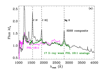
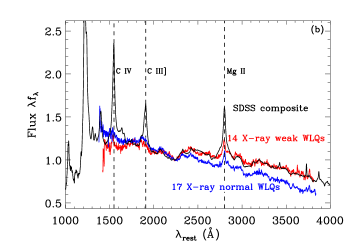
Figure 10.— Comparison of the composite SDSS spectra for the (a) 17 X-ray weak PHL 1811 analogs and PHL 1811 and (b) 14 X-ray weak and 17 X-ray normal WLQs, with the $y$-axis being the flux in arbitrary linear units. In both panels, the SDSS composite spectrum in Vanden Berk et al. (2001) is also shown for comparison. PHL 1811 and its analogs have similar redder continua than the SDSS composite spectrum, with PHL 1811 having stronger UV Fe ii (2250–2650 Å) emission. The X-ray weak WLQs have generally redder continua than the SDSS composite spectrum, while the X-ray normal WLQ composite spectrum is bluer and also exhibits weaker UV Fe ii emission.

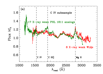
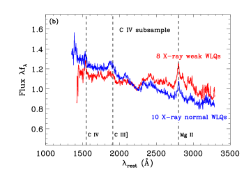
Figure 11.— Comparison of the composite SDSS spectra for the (a) 17 X-ray weak PHL 1811 analogs and 8 X-ray weak WLQs and (b) 8 X-ray weak and 10 X-ray normal WLQs in the C iv subsample. The composite spectra for the X-ray weak PHL 1811 analogs and WLQs are similar to each other. The X-ray weak WLQs have redder continua and stronger UV Fe ii (2250–2650 Å) emission than the X-ray normal WLQs.

To check the reliability of our approach for creating composite spectra, we made a composite spectrum for the 7251 SDSS quasars satisfying the redshift, magnitude, radio-loudness, and non-BAL criteria of PHL 1811 analogs (Section 2.1), and it agrees very well with the Vanden Berk et al. (2001) SDSS quasar composite spectrum in the 1500–3500 Å range. In addition, to check whether the redder color [$\Delta(g-i)=0.24$] of the 17 X-ray weak PHL 1811 analogs is an outcome of small sample bias, we randomly picked 17 SDSS quasars from the above sample and measured the $\Delta(g-i)$ value of their composite spectrum. This practice was repeated 10 000 times and the resulting $\Delta(g-i)$ distribution has an rms scatter of 0.037. Therefore, the redder color of the PHL 1811 analogs is a highly significant (6.4$\sigma$) result.

The composite SDSS spectra for the 14 X-ray weak and 17 X-ray normal WLQs are shown in Figure 10b, with comparison to the SDSS quasar composite spectrum. Similar to the PHL 1811 analogs, the X-ray weak WLQs have weak C iv, C iii], and Mg ii emission lines but normal UV Fe iii and Fe ii emission, compared to the SDSS composite spectrum. The X-ray weak WLQs have generally redder continua than the SDSS composite spectrum, with $\Delta(g-i)=0.11$. The X-ray normal WLQ composite spectrum is bluer than the SDSS composite spectrum, with $\Delta(g-i)=-0.11$. It also has weaker UV Fe ii emission than the X-ray weak WLQ or SDSS composite spectra (more evident in Figures 12 and 13 below).

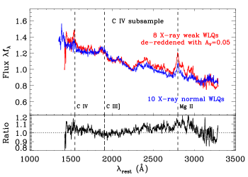
Figure 12.— Composite SDSS spectrum for the eight X-ray weak WLQs de-reddened with $A_{V}=0.05$ mag compared to the composite spectrum for the 10 X-ray normal WLQs in the C iv subsample. The bottom panel shows the ratio of the two spectra. The de-reddening was performed assuming an SMC extinction law. The de-reddened X-ray weak composite spectrum matches well with the X-ray normal composite spectrum, except for some excess UV Fe ii and Mg ii emission.

Composite spectra were also made for the C iv subsample. In Figure 11, we compare the composite spectra for the X-ray weak PHL 1811 analogs, X-ray weak WLQs, and X-ray normal WLQs in the C iv subsample. These spectra are similar to the corresponding composite spectra for the full sample. The composite spectra for the X-ray weak PHL 1811 analogs and WLQs are similar to each other. The X-ray weak WLQs have redder continua and stronger UV Fe ii (2250–2650 Å) emission than the X-ray normal WLQs.

We de-reddened the composite spectrum for the X-ray weak WLQs with various $A_{V}$ values to test whether the difference between the X-ray weak and X-ray normal composite spectra can be explained by dust extinction. A Small Magellanic Cloud (SMC) extinction law (Gordon et al. 2003; $R_{V}=2.74$) was adopted which is usually used to describe intrinsic quasar reddening (e.g., Hopkins et al., 2004; Glikman et al., 2012). As shown in Figure 12, mild dust extinction of $A_{V}=0.05$ mag could describe well the redder composite spectrum for the X-ray weak WLQs, with the remaining residuals mainly in the UV Fe ii and Mg ii emission. This small amount of dust reddening corresponds to a gas column density of $N_{\rm H}<10^{20}$ cm^-2 assuming a Galactic gas-to-dust ratio (e.g., Güver & Özel, 2009), and thus the extra dust for the reddening cannot explain the observed X-ray weakness which requires $N_{\rm H}\approx 10^{24}$ cm^-2 (Section 4.1). This simple testing of reddening cannot, of course, exclude the possibility of an intrinsically redder spectrum for the X-ray weak WLQs.

5.5. Spectral Diagnostics of X-ray Weak Quasars

Studies of the composite SDSS spectra revealed distinct characteristics of our X-ray weak PHL 1811 analogs and WLQs with respect to the X-ray normal population, including redder continua and stronger UV Fe ii emission. We thus performed a statistical analysis of various emission-line and continuum properties, searching for possible spectral diagnostics of X-ray weak quasars that would help reveal their nature.

We ran Peto-Prentice tests to assess whether the distributions of the optical–UV spectral properties of the X-ray weak objects differ from those of the X-ray normal objects. We combined PHL 1811 analogs and WLQs in these tests considering that they can be unified (W11; see also Section 6 below). We examined the C iv REW, C iv blueshift, C iv FWHM, REWs of the $\lambda 1900$, Fe ii, Fe iii, and Mg ii emission features, and also the relative SDSS color $\Delta(g-i)$. The tests were performed for both the full sample and the C iv subsample; the results are shown in Table 6.

We found that statistically, the X-ray weak PHL 1811 analogs and WLQs have larger Fe ii REWs and redder $\Delta(g-i)$ colors than the X-ray normal objects, both at the more than 3$\sigma$ significance level (3.8$\sigma$ and 4.6$\sigma$). The significance levels of the differences drop slightly (to 2.9$\sigma$ and 3.7$\sigma$) for the C iv subsample, probably due to the smaller sample size. For the other spectral properties in either the full sample or the C iv subsample, discrepancies are found at the 1.2–2.7$\sigma$ level: the X-ray weak population has in general stronger C iv blueshifts (1.7$\sigma$), larger C iv FWHMs (2.2$\sigma$), and higher UV emission-line REWs (e.g., C iv REW at 2.3$\sigma$) than the X-ray normal population.

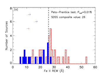
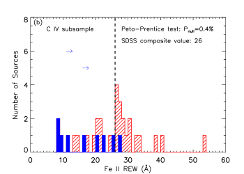
Figure 13.— Distributions of the Fe ii REWs for the (a) full sample and (b) C iv subsample. The hatched red and solid blue shaded histograms and arrows (representing limits) are for the X-ray weak and X-ray normal objects, respectively. We list the probability of the two distributions being drawn from the same parent population based on the Peto-Prentice test. We also list, and plot as the vertical dashed line, the Fe ii REW measured from the SDSS composite spectrum in Vanden Berk et al. (2001). The X-ray weak objects have on average larger Fe ii REWs than the X-ray normal objects.

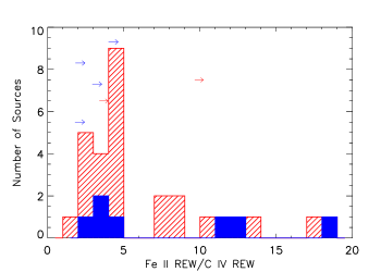
Figure 14.— Distribution of the Fe ii REW to C iv REW ratios for the X-ray weak (red) and X-ray normal (blue) objects. The X-ray weak and normal objects have similar distributions of these line ratios, and the Peto-Prentice test also suggests no significant difference ($P_{\rm null}=0.5$).

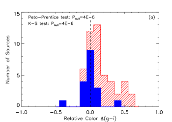
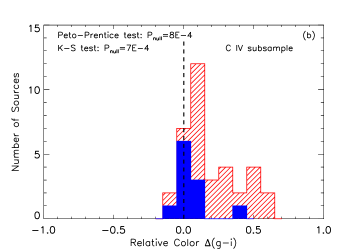
Figure 15.— Distributions of the relative color, $\Delta(g-i)$, for the (a) full sample and (b) C iv subsample. The hatched red and solid blue shaded histograms represent X-ray weak and X-ray normal objects, respectively. The vertical dashed line indicates a relative color of zero. The probabilities of the two distributions being drawn from the same parent population based on the Peto-Prentice test and K-S test are listed. The X-ray weak objects are in general redder than the X-ray normal objects and typical SDSS quasars.

We consider the UV Fe ii REW and $\Delta(g-i)$ color as the most significant diagnostics of X-ray weak PHL 1811 analogs and WLQs. The distributions of the Fe ii REWs for the X-ray weak and X-ray normal populations are shown in Figure 13, with the results from the Peto-Prentice test listed. The Fe ii REW measured from the SDSS quasar composite spectrum is also plotted for comparison. The X-ray weak objects have in fact comparable UV Fe ii emission to typical SDSS quasars, while the X-ray normal objects have weaker than average Fe ii emission. This result is consistent with the findings from the composite spectra (Section 5.4). We also compared the distributions of the Fe ii to C iv REW ratio for the 24 X-ray weak and 11 X-ray normal objects with both Fe ii REW and C iv REW constraints (Figure 14), and no significant difference was found (Peto-Prentice test $P_{\rm null}=0.5$).

The distributions of the $\Delta(g-i)$ colors are shown in Figure 15, with the results from the Peto-Prentice test and Kolmogorov-Smirnov (K-S; applicable when there are not censored data) test listed. The median $\Delta(g-i)$ color for the X-ray weak population is 0.17, and it is 0.01 for the X-ray normal population. In the C iv subsample, these values are 0.23 and 0.03, respectively. These color offsets are modest, and as pointed out in Section 2.4 of W11, the PHL 1811 analogs and WLQs are still within the inclusion area for the SDSS color selection of quasars (e.g., Richards et al., 2002).

Figure 16 displays how the X-ray weak and X-ray normal sample objects are separated in the relative color vs. Fe ii REW plot. The normal X-ray emission from J1537+2716, the only X-ray normal PHL 1811 analog, can be explained by its small $\Delta(g-i)$ and Fe ii REW (estimated to be $13\pm 2$ Å based on the fractional coverage; Table 2) values. There is also one obvious outlier in Figure 16, J0844+1245, that has an unusually red color, $\Delta(g-i)=0.37$, yet is X-ray normal. This source has a relatively high radio loudness parameter and it is possible that its X-ray emission has some contribution from jet-linked emission (see more details in Section 4.3).

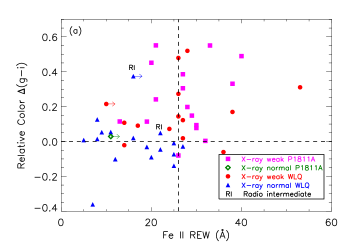
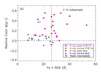
Figure 16.— Relative color vs. Fe ii REW for the (a) full sample and (b) C iv subsample, including the X-ray weak PHL 1811 analogs (magenta squares), X-ray normal PHL 1811 analog (green diamond), X-ray weak WLQs (red circles), and X-ray normal WLQs (blue triangles). The X-ray normal PHL 1811 analog has an estimated Fe ii REW of $13\pm 2$ Å based on the fractional coverage of Fe ii (Table 2). The dashed lines represent the median SDSS color and the Fe ii REW in the SDSS composite spectrum. We also mark two objects, J0844+1245 and J1156+1848, that are considered radio intermediate ($R>10$) in the Shen et al. (2011) SDSS quasar catalog using a slightly different definition of $R$ from the one used here (Section 4.3). The WLQs and PHL 1811 analogs that have redder colors and/or larger Fe ii REWs than the average SDSS values are more likely to be X-ray weak quasars.

The X-ray weakness of our sample objects is measured by the $\Delta\alpha_{\rm OX}$ parameter. Due to the significant fraction of sources not detected in the X-rays, it is not feasible to perform correlation analysis between $\Delta\alpha_{\rm OX}$ and Fe ii REW or $\Delta(g-i)$. Instead, we utilized the Kendall’s $\tau$ and Spearman’s rank-order tests in the ASURV package to check whether such a correlation exists. These tests were performed on the C iv subsample, and the distributions of the quantities are plotted in Figure 17. The resulting small null-hypothesis probabilities (0.2%–1%) suggest a likely correlation between $\Delta\alpha_{\rm OX}$ and Fe ii REW or relative color, and the overall trend is such that a larger Fe ii REW or $\Delta(g-i)$ corresponds to a smaller $\Delta\alpha_{\rm OX}$. We also show the stacked data points in Figure 17 for the 15 Chandra undetected sources (excluding the two XMM-Newton undetected sources), which have a mean $\Delta\alpha_{\rm OX}$ of $-0.99$ following the stacking procedure in Section 5.1. Deeper X-ray observations, converting the $\Delta\alpha_{\rm OX}$ upper limits into detections (factors of $\approx 10$ increase in the exposure times are needed given the stacked X-ray flux level), or a larger sample is required to quantify the possible correlations.

It is also of interest to probe the correlation between the spectral properties and $\alpha_{\rm OX}$, which is an indicator of the X-ray flux level. In the C iv subsample, the objects have a narrow distribution in $L_{\rm 2500~{}{\textup{\AA}}}$ (within about an order of magnitude) and thus a narrow range of expected $\alpha_{\rm OX}$ values (within $\sim 0.14$) from the Just et al. (2007) $\alpha_{\rm OX}$–$L_{\rm 2500~{}{\textup{\AA}}}$ relation. Therefore, replacing $\Delta\alpha_{\rm OX}$ with $\alpha_{\rm OX}$ in Figure 17 does not change the distributions significantly, and similar trends still exist in the sense that a larger Fe ii REW or $\Delta(g-i)$ corresponds to a smaller $\alpha_{\rm OX}$.

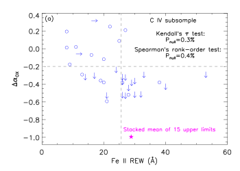
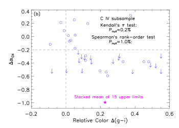
Figure 17.— $\Delta\alpha_{\rm OX}$ vs. (a) Fe ii REW and (b) relative color for the C iv subsample. The horizontal gray dashed lines represent the division between X-ray weak and X-ray normal quasars in this study. The vertical gray dashed lines display the Fe ii REW in the SDSS composite spectrum and the median SDSS color, respectively. For the undetected 15 objects with Chandra data (the other two undetected sources have XMM-Newton observations) in this figure, we show their stacked $\Delta\alpha_{\rm OX}$ value and the mean Fe ii REW (or relative color) as the magenta star. We performed both the Kendall’s $\tau$ and Spearman’s rank-order tests in the ASURV package for correlation analyses. These tests work with data having upper and/or lower limits, and the resulting small null-hypothesis probabilities (0.2%–1%) suggest significant correlations between $\Delta\alpha_{\rm OX}$ and Fe ii REW or relative color.

5.6. Selection Bias in the X-ray Weak Quasar Diagnostics?

We found that X-ray weak PHL 1811 analogs and WLQs generally have larger Fe ii REWs, as well as larger C iv blueshifts, C iv FWHMs, and UV line (C iv, the $\lambda 1900$ complex, Fe iii, and Mg ii) REWs at a less significant level, than the X-ray normal population. However, PHL 1811 analogs and WLQs were mixed to form a large sample for statistical analysis, which could in fact introduce a selection effect due to the different selection criteria for these two types of objects. As detailed in Section 2, the PHL 1811 analogs were selected with a less stringent requirement on the C iv REW, and no requirements on the REWs of the $\lambda 1900$ complex and Mg ii, but with extra requirements on the C iv blueshift and UV Fe ii and Fe iii strength. The fraction of X-ray weak quasars is significantly higher among the PHL 1811 analogs than the WLQs, and X-ray weak PHL 1811 analogs also constitute a substantial fraction ($>50\%$) of the X-ray weak population analyzed here. A consequence is that all the above criteria would stand out as spectral diagnostics of X-ray weak quasars in our analysis while only one or some of these might really be responsible for the weak X-ray emission.

To avoid this possible selection bias, we performed the tests in Section 5.5 using only the WLQs in the C iv subsample, which has eight X-ray weak and 10 X-ray normal objects. Not all of these objects have measurements of all the emission-line properties. Only three properties in Table 6 differ at the more than 1.5$\sigma$ significance level between the X-ray weak and X-ray normal populations: Fe ii REW (2.0$\sigma$), Mg ii REW (1.6$\sigma$), and $\Delta(g-i)$ (2.7$\sigma$). The less-significant test results could either be due to the selection bias being removed or simply the smaller sample size. The latter effect is evident in the $\Delta(g-i)$ results (3.7$\sigma$ to 2.7$\sigma$), which are not affected by the selection bias. Nevertheless, Fe ii REW and $\Delta(g-i)$ remain the most robust diagnostics of X-ray weak quasars.

It is also possible that the relatively larger REWs of the UV lines (e.g., C iv) of the X-ray weak population are real instead of being a selection effect, if they are intrinsically connected with the relatively larger Fe ii REW, e.g., in the shielding-gas scenario discussed in Section 6.4 below. With our currently limited sample of X-ray observed WLQs, it is difficult to assess whether there is a selection bias in the diagnostic analysis.

6. DISCUSSION

6.1. Unification of PHL 1811 Analogs and WLQs with the Shielding-Gas Scenario

The overall similarities between the X-ray weak PHL 1811 analogs and WLQs, including their IR–UV SEDs (Figures 7 and 8), composite SDSS spectra (Figure 11), and degrees of X-ray weakness (Figure 5), suggest that PHL 1811 analogs and WLQs are physically similar types of object. PHL 1811 analogs are empirically a subset of WLQs (with small differences caused by the differing selection approaches; Sections 2.1 and 2.2), and with the additional requirements of PHL 1811-like emission-line properties, we preferentially selected X-ray weak WLQs as the PHL 1811 analogs. Given our analysis of the X-ray weak quasar diagnostics in Section 5.5, the criterion of strong UV Fe ii emission most likely influenced this outcome, while the criteria of large C iv blueshift and strong UV Fe iii emission might also play a role.

Based on the properties of the small pilot sample of PHL 1811 analogs, W11 proposed a simple shielding-gas scenario to unify PHL 1811 analogs (X-ray weak WLQs) and X-ray normal WLQs. In this model, the shielding gas has a sufficiently high covering factor to shield all or most of the BELR from the ionizing continuum, resulting in the observed weak UV emission lines. Whether we observe an X-ray weak or X-ray normal quasar is then an orientation effect, depending upon whether our line of sight intersects the X-ray absorbing shielding gas. X-ray normal WLQs are observed at small inclination angles, while X-ray weak WLQs and PHL 1811 analogs are observed at larger inclination angles.

With our extended sample of PHL 1811 analogs and WLQs, the spectral stacking results suggest that the X-ray weak objects are generally absorbed instead of being intrinsically X-ray weak (Section 5.1). The presence of the significant fraction of X-ray normal WLQs ($\approx 50\%$) also indicates that the weak UV line emission in PHL 1811 analogs and WLQs cannot universally be attributed to intrinsic X-ray weakness. The average X-ray weakness factor for our X-ray weak PHL 1811 analogs or WLQs in the C iv subsample is $\approx 40$, corresponding to $N_{\rm H}\approx 9\times 10^{23}$ cm^-2 (Section 4.1). The spectral analysis of J1521+5202 also revealed strong X-ray absorption with $N_{\rm H}=(1.26_{-0.46}^{+0.54})\times 10^{23}$ cm^-2 (Section 3.2). We note that the actual $N_{\rm H}$ values could be much larger if the observed X-ray emission is dominated by reflected/scattered X-rays rather than direct transmission (e.g., Murphy & Yaqoob, 2009); a substantial contribution from reflected/scattered X-rays is expected for such levels of X-ray weakness based on observations of, e.g., local Seyfert 2 galaxies. These findings provide further support for the W11 shielding-gas scenario, where a soft ionizing continuum due to small-scale absorption is the key for creating the BELR line properties of PHL 1811 analogs and WLQs.

It has been suggested that the FWHMs of low-ionization lines (e.g., H$\beta$, Mg ii) have an orientation dependence due to a flattened BELR geometry (e.g., Wills & Browne, 1986; Runnoe et al., 2013; Shen & Ho, 2014), with the FWHMs generally being larger at larger inclination angles (although there is considerable object-to-object scatter). There are 23 X-ray weak objects and 17 X-ray normal objects in our sample having Mg ii FWHM measurements in the Shen et al. (2011) catalog. The X-ray weak objects have relatively larger Mg ii FWHMs than the X-ray normal objects (mean FWHM values $5400\pm 600$ km s^-1 vs. $4100\pm 600$ km s^-1 and median values $5300$ km s^-1 vs. $2900$ km s^-1), consistent with the shielding-gas scenario where the X-ray weak objects are viewed at larger inclination angles. However, a K-S test between the two sets of Mg ii FWHMs does not indicate a highly significant difference, so we consider this result only suggestive at present.

One possible consequence of the shielding-gas scenario is that the $\Delta\alpha_{\rm OX}$ distribution of PHL 1811 analogs and WLQs would appear bimodal, at least to first approximation, as the sources are either heavily X-ray absorbed or X-ray normal. Due to the large fraction of undetected sources in the X-ray weak population, the $\Delta\alpha_{\rm OX}$ distributions for our samples (Figure 6) cannot reveal clear bimodality. However, the very large average X-ray weakness factors ($\gtrsim 100$; Section 4.1) for these undetected sources do suggest that the $\Delta\alpha_{\rm OX}$ values cannot have a continuous distribution and bimodality is plausible. Deeper X-ray observations are required to constrain better the $\Delta\alpha_{\rm OX}$ distribution.

Based on the X-ray and multiwavelength properties of PHL 1811 analogs and WLQs, some basic physical requirements on the shielding gas can be obtained:

1. The shielding gas has a large column density of X-ray absorption (at least $10^{23}$ cm^-2 and likely much larger).

2. It lacks accompanying C iv BALs or mini-BALs at least along our line of sight.

3. It lies closer to the SMBH than the BELR, so that it can screen the nuclear EUV and X-ray emission from reaching the BELR. Furthermore, it should have a large covering factor to the BELR.

4. The “waste heat” from the absorbed high-energy emission (that otherwise would have reached the BELR) is likely re-emitted in the unobserved EUV as the continuum IR–UV SED appears normal. Such re-emission in the EUV is indicative of a small-scale absorber on a scale of $\approx 10R_{\rm s}$ ($R_{\rm s}=2GM_{\rm BH}/c^{2}$ is the Schwarzschild radius).

Given these properties, the shielding gas might naturally be understood as a geometrically thick inner accretion disk (e.g., a slim disk; see Section 6.2 below). This would require much of the BELR gas to be in an equatorial configuration, as supported by observations (e.g., Shen & Ho, 2014).

6.2. A Geometrically Thick Disk Scenario for the X-ray Absorbing Shielding Gas

Although the X-ray weak and X-ray normal PHL 1811 analogs and WLQs can be unified under the W11 shielding-gas scenario, the physical nature of this shielding gas, that can produce such quasars with extreme emission-line and X-ray properties, remains mysterious. Based on its physical requirements enumerated above (Section 6.1), we propose that a geometrically thick inner accretion disk may naturally serve as the shielding gas. We discuss below such a scenario in the context of a puffed-up disk due to rapid or even super-Eddington accretion. However, we first note that the basic idea of our model stands irrespective of the exact physical processes leading to the geometrical thickness of the disk.

Given the small fraction of PHL 1811 analogs and WLQs among SDSS quasars, a geometrically thick accretion disk with a sufficiently large scale height to shield the BELR almost fully should be a rare phenomenon. Under our selection criteria for the PHL 1811 analogs, 66 candidates were identified from $\approx 7200$ SDSS quasars satisfying the redshift, magnitude, radio-loudness, and non-BAL requirements (Section 2.1). The corresponding fraction is $\approx 0.9\%$, consistent with the estimation of $\lesssim 1.2\%$ in W11. The fraction of WLQs among SDSS quasars is likely larger by a factor of $\approx 2$ due to the addition of the X-ray normal population. The rarity of these quasars suggests a link to some extreme physical property. One relevant physical quantity is the Eddington ratio, as suggested by earlier studies (e.g., Leighly et al., 2007a, b; Shemmer et al., 2010).

PHL 1811 itself has an estimated Eddington ratio of $\approx 1.6$ (Leighly et al., 2007b). PHL 1811, along with several PHL 1811 analogs and WLQs with rest-frame optical spectra (J1521+5202, 2QZ J2154$-$3056, and the two high-redshift WLQs in Shemmer et al. 2010), have weak or undetected [O iii] $\lambda 5007$ narrow emission lines, suggestive of high Eddington ratios (e.g., Boroson & Green, 1992; Shen & Ho, 2014). Moreover, several studies have found that as $L_{\rm Bol}/L_{\rm Edd}$ increases, the C iv REW generally decreases and the C iv blueshift also increases (e.g., Bachev et al., 2004; Baskin & Laor, 2004; Richards et al., 2011; Shen & Ho, 2014; Sulentic et al., 2014; Shemmer & Lieber, 2015). In these correlations, there is only limited sampling in the super-Eddington or low ($<10$ Å) C iv REW regime, but the overall trends suggest that the Eddington ratio grows as one moves from typical quasars toward WLQs in the C iv REW vs. blueshift space (Figure 3a). By the nature of our selection of the PHL 1811 analogs and WLQs, demanding that the BELR does not produce normal emission lines, we may have recovered effectively a population of quasars with (extremely) high Eddington ratios. It is difficult to measure $L_{\rm Bol}/L_{\rm Edd}$ directly for our exceptional objects, as the SMBH masses estimated from the line-based virial method are likely highly uncertain and perhaps systematically in error (Section 5.3). However, based on the empirical $\Gamma\textrm{--}L_{\rm Bol}/L_{\rm Edd}$ relations, our joint spectral analysis of the X-ray normal subsample in Sections 5.2 and 5.3 does indicate a high Eddington ratio ($L_{\rm Bol}/L_{\rm Edd}\approx 1$) in general for our quasars.

A high Eddington ratio is naturally connected to our proposed geometrically thick accretion disk. When the Eddington ratio is high ($L_{\rm Bol}/L_{\rm Edd}\gtrsim 0.3$), optically thick advection becomes important and a slim accretion disk (e.g., Abramowicz et al., 1988; Mineshige et al., 2000; Wang & Netzer, 2003; Ohsuga & Mineshige, 2011; Straub et al., 2011; Netzer & Trakhtenbrot, 2014; Wang et al., 2014a, and references therein) is a more appropriate solution than the standard Shakura & Sunyaev (1973) thin accretion disk. The slim disk has a geometrically thick inner region which, in the case of PHL 1811 analogs and WLQs, might act as the shielding gas that blocks the nuclear ionizing continuum from reaching the BELR (e.g., Leighly, 2004; Wang et al., 2014b). Recent three-dimensional global MHD simulations of super-Eddington accretion disks with accurate and self-consistent radiative transfer (Jiang et al. 2014; Y.-F. Jiang 2015, private communication) or MHD simulations of super-Eddington accretion disks accounting for general relativity and magnetic pressure (Sa̧dowski et al., 2014) also show this geometrically and optically thick inner region. An extremely high Eddington ratio is probably required for the inner disk to be puffed up sufficiently to reach the large necessary covering factor to the BELR. This thick inner disk might also block a significant portion of the ionizing radiation from reaching the narrow line region, leading to the observed weak [O iii] emission (e.g., Boroson & Green, 1992). A schematic illustration of this scenario is shown in Figure 18. In order for the puffed-up disk to block the nuclear high-energy emission from reaching the BELR, the disk corona must be fairly compact. Studies of the rapid X-ray variability (e.g., Shemmer et al., 2014; Uttley et al., 2014) and X-ray microlensing (e.g., Dai et al., 2010; Morgan et al., 2012) of AGNs have constrained the sizes of the X-ray emitting regions to $\approx 5R_{\rm s}$ in these systems, consistent with the requirements of our model.

The expected SED from a super-Eddington accretion disk is uncertain. In the optical–UV, it likely has a power-law shape similar to a standard thin accretion disk, but in the FUV to soft X-ray range ($\approx 10$–100 eV), it is probably flatter (e.g., Wang & Netzer, 2003). The nuclear high-energy emission absorbed by the geometrically thick inner disk (the shielding gas) will likely enhance its EUV (e.g., $\approx 50$ eV) emission, and thus the source will appear to have a typical quasar continuum SED from the IR to UV (Section 4.2). The column density through the puffed-up inner accretion disk is high ($N_{\rm H}\gg 10^{24}$ cm^-2), much larger than the average $N_{\rm H}$ of $\approx 9\times 10^{23}$ cm^-2 roughly estimated for our X-ray weak objects (Section 6.1). Therefore, the observed X-ray emission from these objects is likely dominated by indirect, reflected/scattered X-rays instead of transmitted emission through the disk. The nuclear X-ray emission could be Compton reflected by the accretion disk and/or scattered by an ionized scattering medium on a larger scale than the inner disk. A broad range of X-ray weakness factors (e.g., Figure 6) might be expected as the reflection/scattering efficiency varies for individual objects, but the overall levels of X-ray weakness should be high for reflection/scattering dominated spectra so that bimodality in the $\Delta\alpha_{\rm OX}$ distribution is still likely expected (see Section 6.1). If the observed X-ray emission is dominated by reflection, a strong Fe K$\alpha$ emission line with a REW of order 1–2 keV is usually expected (e.g., Ghisellini et al., 1994; Matt et al., 1996), which cannot be constrained with our limited data.

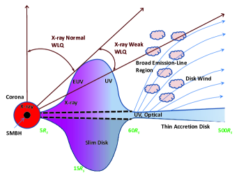
Figure 18.— A schematic diagram of the geometrically thick disk scenario for PHL 1811 analogs and WLQs. When the accretion rate is very high, the inner region of the accretion disk is puffed up significantly, which serves as the shielding gas in the W11 scenario. It blocks the nuclear ionizing continuum from reaching the BELR, resulting in the observed weak line emission. The dashed lines illustrate a standard thin accretion disk, where the BELR is illuminated normally. The inner region of the disk can also absorb the coronal X-ray emission, resulting in an X-ray weak PHL 1811 analog/WLQ when the disk inclination angle is moderate or an X-ray normal object when the inclination angle is small. A standard accretion disk wind is launched from the outer region of the disk. The BELR contains both a static component and a wind component, at least for the C iv line (e.g., Richards et al., 2011). We annotate the approximate scale of the disk in several places, in units of the Schwarzschild radius ($R_{s}$).

If our line of sight is close to the edge of the inner bulge of the puffed-up disk in some objects, a small change in the covering factor of the inner disk due to, e.g., accretion-disk instability could result in transitions between X-ray weak and X-ray normal states on timescales of years. Such a phenomenon may have been observed in the $z=0.396$ quasar PHL 1092. It has similar emission-line properties to PHL 1811 (Leighly et al. 2007a; W11), and it varied between an X-ray normal quasar and an X-ray weak quasar over a timescale of years with a maximum variability factor of $\approx 260$ in its 2 keV flux; meanwhile, its UV emission lines did not show such a drastic change (Miniutti et al., 2009, 2012) as would be expected if the covering-factor change is small. Further X-ray monitoring observations of PHL 1811 analogs and WLQs are required to constrain the frequency and duration of such transitions, which may be a useful probe of the geometrically thick disk scenario.

6.3. Broader Implications of Geometrically Thick Disks for Quasar Emission Lines

Based on our geometrically thick disk scenario for PHL 1811 analogs and WLQs, these extreme and rare quasars are likely not a distinct population, but are instead extreme members of the continuous population of quasars. The shielding effect from a puffed-up inner disk likely exists beyond these extreme objects, and it might be applicable at a milder level to quasars with lower Eddington ratios; in either the slim-disk model or the Jiang et al. (2014) simulations, the disk is unlikely as thin and flat as what a standard disk model describes as long as $L_{\rm Bol}/L_{\rm Edd}\gtrsim 0.3$. When the Eddington ratio is smaller than those of PHL 1811 analogs and WLQs, the radius and scale height of the puffed-up disk decreases, and its covering factor to the BELR also decreases, leading to a larger C iv REW than those of PHL 1811 analogs and WLQs.

Given a continuously varying covering factor of the inner disk that is $L_{\rm Bol}/L_{\rm Edd}$ dependent, a substantial fraction of the quasar C iv REW distribution (spanning about two orders of magnitude; Figure 3a) could be governed by the Eddington ratio. Additional factors shaping this distribution include anisotropic continuum emission, anisotropic line emission, gas metallicity, C iv BELR geometry (setting the fraction of ionizing radiation that is captured), and potential self-shadowing of the BELR (e.g., Korista et al., 1998; Korista & Goad, 2004; Goad et al., 2012; Baskin et al., 2014; Wang et al., 2014b). Furthermore, shielding of the nuclear X-ray emission can prevent the disk wind from being overionized and help the launching of the wind (e.g., Murray et al., 1995; Proga et al., 2000). A larger covering factor of the geometrically thick disk (larger $L_{\rm Bol}/L_{\rm Edd}$) could thus produce a stronger outflowing wind and result in a larger C iv blueshift. The distribution of quasar C iv blueshifts (Figure 3a) could thus also be partly explained by the disk shielding scenario.

6.4. X-ray Weak Quasar Diagnostics and the Shielding-Gas Scenario

We investigated the X-ray weak quasar diagnostics discovered in Section 5.5, and found that they can be plausibly fitted into the W11 shielding-gas scenario, where the X-ray weak objects are viewed at larger inclination angles than the X-ray normal objects.

The redder $\Delta(g-i)$ color of the X-ray weak population can be explained by mild excess intrinsic reddening ($A_{V}\approx 0.05$ mag; Section 5.4) if the dust tends to reside in the equatorial plane of the quasar (e.g., in a dust-driven outer wind scenario as discussed by Elvis 2012) which leads to more extinction at larger inclination angles. Another possible scenario is that the accretion-disk emission is not isotropic (e.g., from a puffed-up slim disk; see Section 6.2), and less UV emission is received at larger inclination angles, producing an intrinsically redder continuum.

The larger REWs of the UV lines (C iv, the $\lambda 1900$ complex, Fe iii, Fe ii, and Mg ii) in the X-ray weak population compared to those in the X-ray normal population may be a consequence of the aspect dependent effects of accretion-disk emission (e.g., Netzer, 1990; Netzer & Trakhtenbrot, 2014; Wang et al., 2014b). The continuum flux from a standard accretion disk scales approximately as $\cos i(1+2\cos i)$, where $i$ is the inclination angle of the disk (Netzer & Trakhtenbrot, 2014). In the case of a slim disk, the disk continuum emission is significantly anisotropic (e.g., see Figure 4 of Wang et al. 2014b). The emission-line flux, on the other hand, is presumably from a BELR structure which overall emits more isotropically. The resulting line REW thus depends on the inclination angle and may be increased by a factor of a few moving from a small angle for an X-ray normal WLQ to a moderate angle for an X-ray weak WLQ. In this scenario, the ratios of the emission-line REWs for the X-ray weak and X-ray normal populations should not differ significantly. This interpretation is supported by the distributions of the Fe ii to C iv REW ratios for the two populations in our sample (Figure 14), which show no significant difference (Peto-Prentice test $P_{\rm null}=0.5$).

The theoretical angular dependence of disk continuum emission is slightly stronger toward longer wavelength in the UV (e.g., Figure 32 of Netzer 1990). The Fe ii emission is at a longer wavelength than the other studied UV lines except Mg ii, and it is also relatively stronger than the other weak UV lines in WLQs (leading to more reliable measurements). These two factors combined probably cause the Fe ii REW to be the best X-ray weak quasar diagnostic among all the REWs in our analysis (C iv, the $\lambda 1900$ complex, Fe iii, Fe ii, and Mg ii).

The other two less-significant diagnostics of X-ray weak quasars, the C iv blueshift (1.7$\sigma$) and FWHM (2.2$\sigma$), can be generally incorporated in the W11 scenario considering that the C iv line has an accelerating disk-wind origin so that the line may have both a larger blueshift and a larger velocity broadening if our line of sight is more aligned with directions along which the wind is strongly accelerated. A large C iv blueshift was one of the selection criteria for our PHL 1811 analogs, but it appears less efficient than the requirement of large UV Fe ii REW for selecting X-ray weak quasars; the orientation-angle dependence of the line-of-sight wind velocity is probably less significant than the orientation-angle dependence of the line REWs.

7. SUMMARY AND FUTURE WORK

7.1. Summary of Main Results

In this paper, we have presented X-ray and multiwavelength investigations of the nature of a large sample of PHL 1811 analogs and WLQs. The key points from this work are the following:

1. We obtained Chandra exploratory (1.5–9.5 ks) observations of 10 PHL 1811 analogs and 22 WLQs. We also acquired a 40 ks Chandra observation of J1521+5202, a PHL 1811 analog that is one of the most luminous SDSS quasars. We measured their X-ray photometric properties, and performed basic spectral analysis for J1521+5202 which suggests strong intrinsic X-ray absorption. Including the previous samples in W11 and W12, we constructed a large sample of 18 PHL 1811 analogs and 33 WLQs at $z=0.5$–2.9 that have X-ray observations. See Sections 2 and 3.

2. Out of the 18 PHL 1811 analogs, 17 (94%) are X-ray weak; out of the 33 WLQs, 16 (48%) are X-ray weak. The selection criteria of PHL 1811-like emission-line properties worked effectively for finding X-ray weak quasars, and we can accommodate the one X-ray normal PHL 1811 analog based on its SDSS spectral properties. The average X-ray weakness factor for the X-ray weak PHL 1811 analogs or WLQs in the C iv subsample is $\approx 40$. The $\Delta\alpha_{\rm OX}$ distributions of the PHL 1811 analogs and WLQs are significantly different from that of typical quasars. See Section 4.1.

3. We constructed IR–X-ray continuum SEDs for the PHL 1811 analogs and WLQs. Both the X-ray weak and X-ray normal groups have IR–UV continuum SEDs similar to those of typical quasars. See Section 4.2.

4. The stacked effective power-law photon indices for the X-ray weak subsamples are relatively hard ($\Gamma_{\rm eff}\approx 0.8$–1.5). These, together with the strong X-ray absorption found in J1521+5202, suggest that the X-ray weak PHL 1811 analogs and WLQs on average are X-ray absorbed, although the possibility of intrinsic X-ray weakness cannot be completely excluded for some objects. See Section 5.1.

5. We performed joint spectral fitting for the 18 X-ray normal PHL 1811 analogs and WLQs. The best-fit hard X-ray photon indices are $\Gamma=2.18\pm 0.09$ for the 18 objects and $\Gamma=2.26\pm 0.11$ for the 10 objects in the C iv subsample, suggesting a high Eddington ratio in general for these X-ray normal objects (and also the X-ray weak objects as they can be unified). See Sections 5.2 and 5.3.

6. We compared composite SDSS spectra for the X-ray weak and X-ray normal PHL 1811 analogs and WLQs, and investigated their optical–UV spectral properties as diagnostics for identifying X-ray weak quasars. Statistically, the X-ray weak PHL 1811 analogs and WLQs have significantly ($>3\sigma$) larger UV Fe ii REWs and redder $\Delta(g-i)$ colors than the X-ray normal population. They also have in general larger C iv blueshifts and FWHMs, and larger UV line (C iv, the $\lambda 1900$ complex, Fe iii, and Mg ii) REWs at a less significant level, than the X-ray normal population. The normal X-ray emission from J1537+2716, the only X-ray normal PHL 1811 analog, can be understood given its small $\Delta(g-i)$ and Fe ii REW. See Sections 5.4–5.6.

7. The PHL 1811 analogs empirically appear to be a subset of WLQs in general, and these two groups of objects can be unified under the W11 shielding-gas scenario. Due to the additional requirements of PHL 1811-like emission-line properties, we preferentially selected X-ray weak WLQs as the PHL 1811 analogs. The X-ray absorption found in J1521+5202 and our stacking results provide further support for the W11 shielding-gas scenario. See Section 6.1.

8. With the requirement of small C iv REWs for PHL 1811 analogs and WLQs, we may have selected effectively a population of quasars with geometrically thick inner accretion disks that can block the ionizing continuum from reaching the BELR and act naturally as the shielding gas of the W11 scenario. These quasars probably have unusually high Eddington ratios so that the inner disk is significantly puffed up (e.g., a slim disk). See Section 6.2.

9. PHL 1811 analogs and WLQs are likely not a distinct population, but are extreme members of the continuous population of quasars. Shielding of the BELR by a geometrically thick disk is thus perhaps generally applicable to quasars with lower Eddington ratios, governing substantial fractions of the observed broad distributions of quasar C iv REWs and blueshifts shown in Figure 3a. See Section 6.3.

7.2. Future Work

Further investigations are needed to test the ideas in this study. We suggested a geometrically thick disk scenario to explain the nature of PHL 1811 analogs and WLQs and to unify these objects. If these quasars are indeed systems with unusually high Eddington ratios, we would expect a larger fraction of them at higher redshifts, as the quasar Eddington ratio generally grows as redshift increases (e.g., Netzer & Trakhtenbrot, 2007; Shen & Kelly, 2012). WLQs do appear to be more common at higher redshifts from studies of limited WLQ samples at $z\approx 3$–6 (Diamond-Stanic et al., 2009; Bañados et al., 2014). To test further this notion, a large sample of WLQs selected systematically across a broad range of redshift is required.

However, there is no simple way to define universal selection criteria for WLQs at all redshifts based solely on SDSS spectroscopy due to the limited spectral coverage (e.g., Section 3.2 of W12). Broader spectral coverage, such as NIR spectra for high-redshift WLQs and UV spectra for low-redshift WLQs, are needed to study the correlations of weak emission lines and thus define consistent selection criteria for WLQs at different redshifts. Currently, only a small sample of WLQs have such broad spectral coverage (e.g., Shemmer et al. 2010; Plotkin et al. 2015), and NIR/UV spectroscopic observations of more WLQs are needed. Moreover, given the unified nature of PHL 1811 analogs and WLQs, the WLQ selection criteria (REW $\lesssim 5$ Å for all emission features) should be relaxed to C iv REW $\lesssim 10$ Å, which will allow the selection of a WLQ sample that is more consistent with the selection of PHL 1811 analogs.

If the distributions of quasar C iv REWs and blueshifts (Figure 3a) are indeed partly the result of the varying covering factor of a geometrically thick disk (which depends on the Eddington ratio) as we suggest in Section 6.3, we would also expect to see more quasars in general having smaller C iv REWs and larger C iv blueshifts at higher redshifts due to the redshift evolution of the quasar Eddington ratio. Caution should be applied when performing such analyses as the C iv REWs and blueshifts might have other luminosity and/or redshift dependences (e.g., the Baldwin effect).

The most-luminous quasar at $z>6$ discovered recently is also a WLQ (Wu et al., 2015), consistent with our expectation that the WLQ fraction rises with redshift. It probably has a high or even super-Eddington accretion rate, as we propose for WLQs (Section 6); a luminosity exceeding the Eddington limit may help explain its very high luminosity. This quasar has a Mg ii-based virial mass of $\approx 1.2\times 10^{10}~{}M_{\sun}$ (Wu et al., 2015). However, as we discussed in Section 5.3, virial-mass estimates for these extreme quasars are highly uncertain and perhaps systematically in error (e.g., Mg ii-based virial masses are on average $\approx 3$ times larger than H$\beta$-based virial masses for five of our objects); this factor could alleviate the challenge of growing such a massive black hole in the early universe. A Chandra observation has been scheduled for this WLQ (PI: X. Fan). Our X-ray results on WLQs suggest there is a $\approx 50\%$ chance that this quasar is X-ray weak. This chance is likely higher based on this object’s relatively red continuum, with a spectral index of $\alpha_{\lambda}=-1.43$ (Wu et al., 2015) as compared to the average spectral index of $\alpha_{\lambda}=-1.72$ for SDSS quasars (e.g., Section 3.2 of Krawczyk et al. 2015). Quantification that its UV Fe ii emission is strong would increase this chance further (see Section 5.5).

Due to the substantial uncertainties in the SMBH mass estimates, it is challenging to measure quantitatively the Eddington ratios of PHL 1811 analogs and WLQs. However, the Eddington ratio appears to be the primary driver of quasar Eigenvector 1 (e.g., Boroson & Green, 1992; Netzer & Trakhtenbrot, 2007; Shen & Ho, 2014), which is dominated by the optical Fe ii/H$\beta$ ratio, [O iii] REW, and H$\beta$ FWHM. NIR spectroscopy of a large sample of WLQs could provide measurements of these emission-line properties in the rest-frame optical. If they indeed have very high Eddington ratios, clustering is expected toward high Fe ii/H$\beta$, low [O iii] REW, and low H$\beta$ FWHM, relative to quasars with comparable luminosities; there are already hints of such clustering based on a small sample of five WLQs (see Section 5.1 of Plotkin et al. 2015). Moreover, the Jiang et al. (2014) and Sa̧dowski et al. (2014) simulations of super-Eddington accretion disks predict a radiation-driven outflow along the rotation axis. Signatures of this outflow may be sought in our X-ray normal WLQs as high-ionization absorption lines/edges at X-ray and UV wavelengths (e.g., O vi absorption, as discussed in Section 4.4 of W11).

To quantify the possible correlations between $\Delta\alpha_{\rm OX}$ and Fe ii REW or $\Delta(g-i)$ (Figure 17) and probe the underlying physics, deeper X-ray observations of the undetected objects are required. Given the stacked X-ray flux level, most of the undetected sources should be detectable with factors of $\approx 10$ increase in the exposure times. Such observations will also help test whether the $\Delta\alpha_{\rm OX}$ distribution is bimodal, as might be expected in the shielding-gas scenario (Section 6.1). Moreover, long-term X-ray monitoring observations of the PHL 1811 analogs and WLQs will be useful, as they can constrain the frequency and duration of the X-ray state transitions as in PHL 1092, and thus provide insights into the geometrically thick disk scenario.

Finally, it remains somewhat perplexing that at least many of our PHL 1811 analogs appear to be X-ray absorbed, while PHL 1811 itself appears intrinsically X-ray weak; Occam’s razor would initially favor a single explanation for the X-ray weakness of all these objects selected to have similar UV emission-line properties. It is worth noting that our PHL 1811 analogs are generally being observed in the $\approx 1.5$–24 keV rest-frame band, while the X-ray properties of PHL 1811 itself have only been effectively probed up to $\approx 8$ keV. Perhaps PHL 1811 itself has a highly absorbed component that has yet to be recognized. Although PHL 1811 has not been detected in the Swift-BAT all-sky survey in the 14–24 keV band (M. Koss 2014, private communication), a NuSTAR observation could probe more sensitively for a highly absorbed component.

We thank M. Eracleous, Y.-F. Jiang, K. Korista, H. Netzer, A. E. Scott, and J. M. Wang for helpful discussions. We thank the referee for carefully reviewing the manuscript and providing helpful comments. We acknowledge financial support from Chandra X-ray Center grant GO3-14100X (B.L., W.N.B.), NASA ADP grant NNX10AC99G (B.L., W.N.B.), ACIS team contract SV4-74018 (B.L., W.N.B.), the V.M. Willaman Endowment (B.L., W.N.B.), NSERC (P.B.H.), and Smithsonian Astrophysics Observatory contract SV2-82024 (G.P.G.).

Funding for the SDSS and SDSS-II has been provided by the Alfred P. Sloan Foundation, the Participating Institutions, the National Science Foundation, the U.S. Department of Energy, the National Aeronautics and Space Administration, the Japanese Monbukagakusho, the Max Planck Society, and the Higher Education Funding Council for England. The SDSS Web Site is http://www.sdss.org/.

Table 1New Chandra Observations and X-ray Photometric Properties

Object Name	Redshift	Observation	Observation	Exposure	Soft Band	Hard Band	Band	$\Gamma_{\rm eff}$	Comment
(J2000)		ID	Start Date	Time (ks)	(0.5–2 keV)	(2–8 keV)	Ratio
(1)	(2)	(3)	(4)	(5)	(6)	(7)	(8)	(9)	(10)
PHL 1811 Analogs
$014733.58+000323.2$	$2.031$	$14949$	2013 Nov 15	$6.2$	$<2.4$	$3.2_{-1.8}^{+3.2}$	$>1.19$	$<0.6$	…
$082508.75+115536.3$	$1.998$	$14951$	2013 Jun 10	$5.1$	$<2.4$	$<2.5$	$...$	$...$	…
$090809.13+444138.8$	$1.742$	$14950$	2013 Sep 23	$6.8$	$<2.4$	$<2.5$	$...$	$...$	…
$094808.39+161414.1$	$1.805$	$14947$	2013 Jun 10	$3.7$	$2.1_{-1.3}^{+2.7}$	$<2.5$	$<1.42$	$>0.4$	…
$113342.67+114206.2$	$2.052$	$14952$	2014 Feb 08	$9.3$	$<2.4$	$2.1_{-1.4}^{+2.9}$	$>0.70$	$<1.0$	…
$143525.31+400112.2$	$2.267$	$14954$	2013 Sep 04	$6.9$	$7.3_{-2.7}^{+3.9}$	$2.1_{-1.4}^{+2.9}$	$0.29_{-0.22}^{+0.43}$	$1.8_{-0.8}^{+1.3}$	…
$152156.48+520238.5$	$2.238$	$15334$	2013 Oct 22	$37.1$	$43.5_{-6.7}^{+7.8}$	$47.9_{-7.3}^{+8.5}$	$1.10_{-0.24}^{+0.28}$	$0.6_{-0.2}^{+0.2}$	W11, archival 4 ks obs.
$153412.68+503405.3$	$2.122$	$14956$	2013 Dec 31	$6.1$	$<4.1$	$<4.2$	$...$	$...$	…
$153714.26+271611.6$	$2.457$	$14955$	2013 Dec 22	$6.0$	$44.4_{-6.8}^{+7.9}$	$22.0_{-4.9}^{+6.1}$	$0.49_{-0.13}^{+0.16}$	$1.3_{-0.3}^{+0.3}$	…
$153913.47+395423.4$	$1.934$	$14948$	2013 Dec 13	$5.3$	$<2.4$	$<2.5$	$...$	$...$	…
$222256.11-094636.2$	$2.913$	$14953$	2013 Sep 27	$9.4$	$2.0_{-1.3}^{+2.7}$	$<4.2$	$<2.87$	$>-0.2$	…
Weak-line Quasars
$014333.65-391700.1$	$1.800$	$15358$	2012 Nov 21	$3.0$	$15.6_{-4.0}^{+5.2}$	$7.7_{-2.8}^{+4.2}$	$0.49_{-0.22}^{+0.31}$	$1.4_{-0.4}^{+0.5}$	HE 0141-3932
$082722.73+032755.9$	$2.031$	$15342$	2013 Mar 23	$2.5$	$<2.4$	$<2.5$	$...$	$...$	…
$084424.24+124546.5$	$2.492$	$15337$	2013 Apr 01	$1.5$	$51.2_{-7.3}^{+8.4}$	$11.0_{-3.4}^{+4.7}$	$0.21_{-0.07}^{+0.10}$	$2.1_{-0.3}^{+0.4}$	…
$090843.25+285229.8$	$0.933$	$15352$	2013 Feb 25	$2.0$	$40.6_{-6.5}^{+7.6}$	$7.7_{-2.8}^{+4.2}$	$0.19_{-0.08}^{+0.11}$	$2.2_{-0.4}^{+0.5}$	…
$100517.54+331202.8$	$1.802$	$15351$	2013 Mar 01	$3.0$	$<4.1$	$<2.5$	$...$	$...$	…
$113413.48+001042.0$	$1.487$	$15343$	2013 Feb 19	$2.5$	$<4.1$	$<2.5$	$...$	$...$	…
$115637.02+184856.5$	$1.993$	$15341$	2013 Mar 20	$2.0$	$43.9_{-6.7}^{+7.9}$	$11.0_{-3.4}^{+4.7}$	$0.25_{-0.09}^{+0.12}$	$2.0_{-0.3}^{+0.4}$	…
$130312.89+321911.4$	$0.638$	$15350$	2012 Nov 19	$2.0$	$<2.4$	$<2.5$	$...$	$...$	…
$131059.77+560140.2$	$1.285$	$15344$	2013 Apr 10	$2.0$	$18.7_{-4.4}^{+5.5}$	$5.5_{-2.4}^{+3.7}$	$0.29_{-0.14}^{+0.22}$	$1.8_{-0.5}^{+0.6}$	…
$132130.21+481719.1$	$1.409$	$15347$	2013 Feb 19	$2.5$	$<2.4$	$<2.5$	$...$	$...$	…
$132809.59+545452.7$	$2.116$	$15338$	2013 Jul 15	$2.0$	$6.2_{-2.5}^{+3.7}$	$2.2_{-1.4}^{+2.9}$	$0.35_{-0.26}^{+0.52}$	$1.7_{-0.8}^{+1.2}$	…
$133222.62+034739.9$	$1.447$	$15340$	2013 Feb 13	$2.0$	$2.1_{-1.3}^{+2.7}$	$6.6_{-2.6}^{+3.9}$	$3.18_{-2.21}^{+6.15}$	$-0.3_{-0.9}^{+1.1}$	Lensed, BAL
$134601.28+585820.2$	$1.664$	$15336$	2013 Apr 28	$1.5$	$<2.4$	$<2.5$	$...$	$...$	…
$140710.26+241853.6$	$1.668$	$15345$	2012 Nov 19	$2.5$	$<2.4$	$<2.5$	$...$	$...$	…
$141141.96+140233.9$	$1.753$	$15353$	2012 Dec 16	$3.4$	$48.9_{-7.1}^{+8.2}$	$13.2_{-3.8}^{+5.0}$	$0.27_{-0.09}^{+0.11}$	$1.9_{-0.3}^{+0.3}$	…
$141730.92+073320.7$	$1.710$	$15349$	2012 Dec 05	$2.5$	$21.9_{-4.7}^{+5.9}$	$5.5_{-2.4}^{+3.7}$	$0.25_{-0.12}^{+0.18}$	$2.0_{-0.5}^{+0.6}$	…
$142943.64+385932.2$	$0.928$	$15335$	2012 Dec 08	$1.5$	$14.6_{-3.8}^{+5.0}$	$4.4_{-2.1}^{+3.5}$	$0.30_{-0.16}^{+0.26}$	$1.8_{-0.6}^{+0.7}$	…
$144741.76-020339.1$	$1.431$	$15355$	2013 Jan 13	$2.0$	$6.2_{-2.5}^{+3.7}$	$<4.3$	$<0.70$	$>1.0$	…
$162933.60+253200.6$	$1.339$	$15356$	2012 Dec 07	$2.9$	$18.7_{-4.4}^{+5.5}$	$17.6_{-4.4}^{+5.6}$	$0.94_{-0.32}^{+0.41}$	$0.8_{-0.3}^{+0.4}$	…
$164302.03+441422.1$	$1.650$	$15348$	2013 May 30	$3.0$	$40.6_{-6.5}^{+7.6}$	$8.8_{-3.0}^{+4.3}$	$0.22_{-0.08}^{+0.11}$	$2.1_{-0.4}^{+0.4}$	…
$172858.16+603512.7$	$1.807$	$15346$	2013 Jan 05	$2.5$	$15.6_{-4.0}^{+5.2}$	$<4.3$	$<0.29$	$>1.8$	…
$212416.05-074129.8$	$1.402$	$15339$	2012 Nov 20	$1.5$	$13.5_{-3.7}^{+4.9}$	$<4.3$	$<0.35$	$>1.7$	…
$215454.35-305654.3$	$0.494$	$15354$	2012 Dec 13	$2.5$	$<2.4$	$<2.5$	$...$	$...$	2QZ J215454.3-305654

Note. — Cols. (1) and (2): object name in the J2000 equatorial coordinate format and redshift. Cols. (3)–(5): Chandra observation ID, observation start date, and background-flare cleaned effective exposure time in the 0.5–8 keV band. Cols. (6)–(7): Aperture-corrected source counts in the soft (0.5–2 keV) and hard (2–8 keV) bands. An upper limit at a 90% confidence level is given if the source is not detected. Col. (8): ratio between the soft-band and hard-band counts. An entry of “…” indicates that the source is undetected in both bands. Col. (9): 0.5–8 keV effective power-law photon index, derived from the band ratio assuming a power-law spectrum modified with Galactic absorption. An entry of “…” indicates that it cannot be constrained. Col. (10): comments on special objects.

Table 2Quasar UV Emission-Line Measurements from the SDSS Spectra

Object Name	MJD	C iv Blueshift	C iv FWHM	REW	REW	REW	REW	REW	REW
(J2000)		(km s-1)	(km s-1)	C iv	Si iv	$\lambda 1900$ Å	Fe ii	Fe iii	Mg ii
(1)	(2)	(3)	(4)	(5)	(6)	(7)	(8)	(9)	(10)
PHL 1811 Analogs
$014733.58+000323.2$	$51793$	$-6170\pm 440$	$7380\pm 560$	$4.5\pm 0.3$	$<3.0$	$3.8\pm 0.3$	$21\pm 2$	$6.2\pm 0.3$	$12.2\pm 0.6$
$082508.75+115536.3$	$54149$	$-4600\pm 340$	$8100\pm 640$	$5.8\pm 0.3$	$4.0\pm 0.3$	$8.2\pm 0.4$	$26\pm 2$	$5.4\pm 0.4$	$13.1\pm 0.8$
$090809.13+444138.8$	$52312$	$-4250\pm 640$	$5650\pm 460$	$4.1\pm 0.5$	$...$	$7.9\pm 0.5$	$32\pm 3$	$4.8\pm 0.8$	$17.1\pm 1.1$
$094808.39+161414.1$	$54095$	$-3700\pm 380$	$8290\pm 660$	$5.9\pm 0.3$	$...$	$3.7\pm 0.3$	$28\pm 2$	$4.7\pm 0.3$	$16.5\pm 0.5$
$113342.67+114206.2$	$53055$	$-2460\pm 1740$	$2900\pm 240$	$2.6\pm 0.8$	$1.4\pm 1.2$	$4.9\pm 0.9$	$27\pm 2$	$3.4\pm 0.7$	$10.4\pm 1.9$
$143525.31+400112.2$	$52797$	$-2050\pm 440$	$6160\pm 500$	$7.4\pm 0.6$	$3.2\pm 0.5$	$8.3\pm 0.8$	$13\pm 1$	$1.9\pm 0.5$	$...$
$152156.48+520238.5$	$52376$	$-9300\pm 610$	$11700\pm 800$	$9.1\pm 0.6$	$2.7\pm 0.3$	$8.2\pm 0.6$	$21\pm 2$	$7.1\pm 0.6$	$14.9\pm 0.6$
$153412.68+503405.3$	$52401$	$-970\pm 320$	$7610\pm 580$	$8.7\pm 0.5$	$3.1\pm 0.3$	$15.8\pm 0.5$	$40\pm 4$	$7.8\pm 0.4$	$25.6\pm 1.0$
$153714.26+271611.6$	$54180$	$-1310\pm 220$	$6560\pm 520$	$6.0\pm 0.3$	$3.9\pm 0.2$	$8.0\pm 0.3$	$>11$ ($13\pm 2$)	$1.9\pm 0.3$	$...$
$153913.47+395423.4$	$53171$	$-3930\pm 600$	$10570\pm 740$	$6.9\pm 0.5$	$2.2\pm 0.4$	$11.2\pm 0.6$	$30\pm 3$	$5.4\pm 0.4$	$19.9\pm 0.8$
$222256.11-094636.2$	$52206$	$-2570\pm 1300$	$5030\pm 440$	$3.7\pm 0.5$	$5.2\pm 0.9$	$8.7\pm 0.7$	$...$	$<3.0$	$...$
Weak-line Quasars
$014333.65-391700.1$	$...$	$...$	$...$	$...$	$...$	$...$	$...$	$...$	$...$
$082722.73+032755.9$	$52642$	$-1460\pm 520$	$2560\pm 200$	$4.0\pm 0.8$	$<1.1$	$2.5\pm 1.1$	$53\pm 5$	$6.0\pm 0.8$	$22.2\pm 2.1$
$084424.24+124546.5$	$53801$	$-1450\pm 500$	$5870\pm 480$	$5.5\pm 0.5$	$2.1\pm 0.4$	$3.1\pm 0.4$	$>16$ ($26\pm 2$)	$3.9\pm 0.5$	$...$
$090843.25+285229.8$	$53330$	$...$	$...$	$...$	$...$	$...$	$19\pm 1$	$<1.6$	$4.9\pm 0.8$
$100517.54+331202.8$	$53378$	$-2420\pm 1040$	$4020\pm 340$	$5.8\pm 1.0$	$...$	$3.4\pm 1.0$	$24\pm 2$	$2.6\pm 1.3$	$12.5\pm 2.1$
$113413.48+001042.0$	$51630,51658$	$...$	$...$	$...$	$...$	$5.1\pm 0.5$	$38\pm 3$	$3.2\pm 0.5$	$12.9\pm 0.6$
$115637.02+184856.5$	$54180$	$-1790\pm 900$	$3180\pm 260$	$1.2\pm 0.5$	$1.5\pm 0.4$	$5.0\pm 0.8$	$22\pm 2$	$1.8\pm 0.6$	$8.5\pm 1.5$
$130312.89+321911.4$	$53819$	$...$	$...$	$...$	$...$	$...$	$>10$	$...$	$7.3\pm 0.9$
$131059.77+560140.2$	$52791$	$...$	$...$	$...$	$...$	$4.5\pm 0.8$	$12\pm 1$	$1.2\pm 0.5$	$7.3\pm 1.0$
$132130.21+481719.1$	$52759$	$...$	$...$	$...$	$...$	$5.6\pm 1.0$	$27\pm 2$	$3.0\pm 0.9$	$9.3\pm 1.0$
$132809.59+545452.7$	$52724$	$-2560\pm 340$	$3970\pm 300$	$4.4\pm 0.4$	$3.5\pm 0.3$	$3.7\pm 0.5$	$20\pm 2$	$3.5\pm 0.5$	$18.3\pm 2.2$
$133222.62+034739.9$	$52374$	$...$	$...$	$...$	$...$	$4.4\pm 1.1$	$8\pm 1$	$<1.5$	$9.3\pm 0.9$
$134601.28+585820.2$	$52425,52466$	$-4570\pm 760$	$5580\pm 440$	$2.9\pm 0.3$	$...$	$4.8\pm 0.3$	$14\pm 1$	$1.7\pm 0.3$	$12.1\pm 0.5$
$140710.26+241853.6$	$53770$	$-780\pm 600$	$1170\pm 140$	$1.5\pm 0.6$	$...$	$5.4\pm 0.8$	$26\pm 2$	$4.1\pm 0.9$	$10.0\pm 1.2$
$141141.96+140233.9$	$53442$	$-1850\pm 740$	$2420\pm 180$	$2.4\pm 0.9$	$...$	$6.6\pm 0.9$	$27\pm 2$	$5.5\pm 1.2$	$6.0\pm 1.6$
$141730.92+073320.7$	$53499$	$-5470\pm 760$	$3240\pm 260$	$2.0\pm 0.7$	$...$	$4.2\pm 0.8$	$25\pm 2$	$2.8\pm 0.8$	$11.2\pm 1.2$
$142943.64+385932.2$	$52797$	$...$	$...$	$...$	$...$	$...$	$22\pm 2$	$2.3\pm 0.5$	$13.7\pm 0.8$
$144741.76-020339.1$	$52411$	$...$	$...$	$...$	$...$	$6.7\pm 0.7$	$7\pm 1$	$2.8\pm 0.7$	$12.4\pm 1.1$
$162933.60+253200.6$	$53226$	$...$	$...$	$...$	$...$	$9.5\pm 1.0$	$5\pm 1$	$3.2\pm 0.9$	$10.7\pm 1.1$
$164302.03+441422.1$	$52051$	$...$	$...$	$<2.0$	$...$	$<2.0$	$8\pm 1$	$9.8\pm 1.6$	$3.9\pm 1.1$
$172858.16+603512.7$	$51792$	$-2630\pm 720$	$3380\pm 340$	$3.1\pm 0.7$	$2.6\pm 1.1$	$6.2\pm 0.8$	$11\pm 1$	$<1.6$	$5.9\pm 1.6$
$212416.05-074129.8$	$52178,52200$	$...$	$...$	$...$	$...$	$2.6\pm 0.5$	$25\pm 2$	$1.4\pm 0.4$	$12.7\pm 0.5$
$215454.35-305654.3$	$...$	$...$	$...$	$...$	$...$	$...$	$...$	$...$	$...$

Note. — Col. (1): object name. Col. (2): modified Julian date of the SDSS observation; an entry of “…” indicates that no SDSS spectrum is available. In a few cases, two spectra are available, and the average spectrum was used for the measurements. Cols. (3) and (4): blueshift and full width at half maximum (FWHM) of the C iv line. Cols. (5)–(10): REWs (in units of Å) of the C iv $\lambda 1549$, Si iv $\lambda 1397$, $\lambda 1900$ complex, Fe ii (2250–2650 Å), Fe iii UV48 $\lambda 2080$, and Mg ii $\lambda 2799$ emission features. The Si iv $\lambda 1397$ line is a blend of Si iv and O iv], and the $\lambda 1900$ emission is dominated by C iii] $\lambda 1909$ with additional contributions from [Ne iii] $\lambda 1814$, Si ii $\lambda 1816$, Al iii $\lambda 1857$, Si iii] $\lambda 1892$, and several Fe iii multiplets (see Table 2 of Vanden Berk et al. 2001 for details). The UV Fe ii REW was measured between 2250Å and 2650Å; for three objects that do not have full spectral coverage of this range, a lower limit was derived (along with an estimated value in parentheses if the covered fraction is $>60\%$). For the other properties, the measurements were performed the same manner as in W11. The uncertainties have been multiplied by the factors given in the notes of W11 Table 3, and the upper limits are at a 3$\sigma$ confidence level.

Table 3X-ray and Optical Properties

Object Name	$M_{i}$	$N_{\rm H,Gal}$	Count Rate	$F_{\rm X}$	$f_{\rm 2~{}keV}$	$\log L_{\rm X}$	$f_{\rm 2500~{}\textup{\AA}}$	$\log L_{\rm 2500~{}\textup{\AA}}$	$\alpha_{\rm OX}$	$\Delta\alpha_{\rm OX}(\sigma)$	$f_{\rm weak}$	$\Delta(g-i)$	$R$
(J2000)			(0.5–2 keV)	(0.5–2 keV)		(2–10 keV)
(1)	(2)	(3)	(4)	(5)	(6)	(7)	(8)	(9)	(10)	(11)	(12)	(13)	(14)
PHL 1811 Analogs
$014733.58+000323.2$	$-27.91$	$2.90$	$<0.39$	$<0.16$	$<0.68$	$<43.77$	$3.68$	$31.58$	$<-2.20$	$<-0.49(3.32)$	$>18.40$	$0.55$	$<1.0$
$082508.75+115536.3$	$-28.31$	$3.67$	$<0.47$	$<0.19$	$<0.81$	$<43.83$	$4.62$	$31.66$	$<-2.21$	$<-0.48(3.30)$	$>17.95$	$-0.08$	$<1.0$
$090809.13+444138.8$	$-27.26$	$1.66$	$<0.35$	$<0.14$	$<0.56$	$<43.56$	$2.09$	$31.21$	$<-2.14$	$<-0.47(3.25)$	$>17.28$	$0.00$	$<1.9$
$094808.39+161414.1$	$-28.43$	$3.34$	$0.55_{-0.36}^{+0.74}$	$0.22$	$0.90$	$43.80$	$6.59$	$31.74$	$-2.25$	$-0.51(3.51)$	$21.67$	$0.20$	$<0.6$
$113342.67+114206.2$	$-27.52$	$3.32$	$<0.26$	$<0.10$	$<0.45$	$<43.60$	$1.99$	$31.32$	$<-2.17$	$<-0.49(3.34)$	$>18.61$	$0.39$	$<2.3$
$143525.31+400112.2$	$-27.84$	$1.00$	$1.05_{-0.39}^{+0.57}$	$0.42$	$1.89$	$44.32$	$3.32$	$31.62$	$-2.01$	$-0.29(2.00)$	$5.75$	$0.11$	$<1.4$
$152156.48+520238.5$	$-30.22$	$1.58$	$1.17_{-0.18}^{+0.21}$	$0.46$	$0.98$	$44.51$	$19.86$	$32.39$	$-2.42$	$-0.59(4.51)$	$34.73$	$0.24$	$<0.2$
$153412.68+503405.3$	$-28.70$	$1.56$	$<0.67$	$<0.27$	$<1.20$	$<44.05$	$3.69$	$31.61$	$<-2.11$	$<-0.39(2.64)$	$>10.13$	$0.49$	$<1.2$
$153714.26+271611.6$	$-28.67$	$3.06$	$7.45_{-1.14}^{+1.32}$	$2.92$	$10.23$	$45.31$	$5.75$	$31.92$	$-1.82$	$-0.06(0.45)$	$1.43$	$0.03$	$2.6$
$153913.47+395423.4$	$-27.99$	$1.70$	$<0.45$	$<0.18$	$<0.76$	$<43.78$	$3.86$	$31.56$	$<-2.19$	$<-0.48(3.26)$	$>17.39$	$0.09$	$<1.2$
$222256.11-094636.2$	$-28.55$	$4.34$	$0.22_{-0.14}^{+0.29}$	$0.09$	$0.47$	$43.88$	$4.33$	$31.92$	$-2.29$	$-0.52(4.01)$	$23.29$	$0.23$	$<1.3$
Weak-line Quasars
$014333.65-391700.1$	$-29.22$	$1.71$	$5.28_{-1.35}^{+1.74}$	$2.07$	$6.75$	$44.88$	$15.28$	$32.10$	$-2.06$	$-0.27(2.03)$	$4.93$	$...$	$<0.5$
$082722.73+032755.9$	$-27.27$	$3.73$	$<0.97$	$<0.39$	$<1.68$	$<44.16$	$1.68$	$31.24$	$<-1.92$	$<-0.25(1.72)$	$>4.50$	$0.31$	$<2.6$
$084424.24+124546.5$	$-28.17$	$3.81$	$33.58_{-4.77}^{+5.50}$	$13.53$	$74.79$	$45.90$	$3.81$	$31.75$	$-1.42$	$0.32(2.17)$	$0.15$	$0.37$	$8.0$
$090843.25+285229.8$	$-25.10$	$2.46$	$20.28_{-3.23}^{+3.80}$	$8.30$	$23.71$	$44.55$	$1.48$	$30.54$	$-1.46$	$0.11(0.57)$	$0.51$	$-0.03$	$<2.0$
$100517.54+331202.8$	$-26.70$	$1.45$	$<1.38$	$<0.55$	$<2.22$	$<44.19$	$1.38$	$31.06$	$<-1.84$	$<-0.20(1.35)$	$>3.26$	$0.07$	$<2.8$
$113413.48+001042.0$	$-26.48$	$2.63$	$<1.64$	$<0.66$	$<2.39$	$<44.07$	$1.57$	$30.96$	$<-1.85$	$<-0.22(1.11)$	$>3.75$	$0.17$	$<2.4$
$115637.02+184856.5$	$-27.30$	$2.83$	$21.91_{-3.36}^{+3.92}$	$8.78$	$38.74$	$45.49$	$2.04$	$31.31$	$-1.43$	$0.25(1.71)$	$0.22$	$0.05$	$7.4$
$130312.89+321911.4$	$-24.20$	$1.17$	$<1.20$	$<0.48$	$<1.20$	$<43.03$	$1.45$	$30.19$	$<-1.95$	$<-0.43(2.17)$	$>13.09$	$0.21$	$<1.9$
$131059.77+560140.2$	$-26.09$	$1.51$	$9.36_{-2.19}^{+2.77}$	$3.73$	$12.42$	$44.69$	$1.64$	$30.86$	$-1.58$	$0.03(0.17)$	$0.82$	$-0.10$	$<2.3$
$132130.21+481719.1$	$-26.20$	$1.13$	$<0.97$	$<0.39$	$<1.36$	$<43.78$	$1.38$	$30.86$	$<-1.92$	$<-0.31(1.54)$	$>6.26$	$0.12$	$<2.6$
$132809.59+545452.7$	$-27.72$	$1.16$	$3.12_{-1.24}^{+1.86}$	$1.23$	$4.89$	$44.75$	$2.70$	$31.47$	$-1.82$	$-0.12(0.81)$	$2.03$	$-0.09$	$<1.7$
$133222.62+034739.9$	$-26.70$	$1.98$	$1.03_{-0.67}^{+1.37}$	$0.41$	$0.63$	$44.47$	$1.75$	$30.98$	$-2.09$	$-0.46(2.31)$	$15.58$	$0.34$	$<2.2$
$134601.28+585820.2$	$-27.38$	$1.63$	$<1.57$	$<0.63$	$<2.43$	$<44.17$	$3.22$	$31.36$	$<-1.97$	$<-0.28(1.92)$	$>5.37$	$0.11$	$<1.3$
$140710.26+241853.6$	$-26.70$	$1.65$	$<0.97$	$<0.39$	$<1.50$	$<43.96$	$1.50$	$31.03$	$<-1.92$	$<-0.28(1.41)$	$>5.36$	$0.14$	$<2.8$
$141141.96+140233.9$	$-26.56$	$1.43$	$14.42_{-2.10}^{+2.43}$	$5.75$	$22.89$	$45.18$	$1.13$	$30.95$	$-1.42$	$0.21(1.06)$	$0.28$	$-0.03$	$<3.6$
$141730.92+073320.7$	$-26.64$	$2.12$	$8.81_{-1.91}^{+2.37}$	$3.53$	$14.14$	$44.93$	$1.64$	$31.09$	$-1.56$	$0.09(0.60)$	$0.59$	$-0.01$	$<3.0$
$142943.64+385932.2$	$-26.01$	$0.95$	$9.56_{-2.53}^{+3.30}$	$3.81$	$11.02$	$44.37$	$3.57$	$30.91$	$-1.73$	$-0.11(0.55)$	$1.91$	$-0.05$	$<0.9$
$144741.76-020339.1$	$-26.00$	$4.53$	$3.11_{-1.24}^{+1.86}$	$1.25$	$4.46$	$44.31$	$1.69$	$30.96$	$-1.76$	$-0.13(0.64)$	$2.15$	$-0.36$	$<2.3$
$162933.60+253200.6$	$-25.35$	$3.58$	$6.39_{-1.49}^{+1.89}$	$2.51$	$6.44$	$44.87$	$1.05$	$30.70$	$-1.62$	$-0.02(0.12)$	$1.16$	$0.01$	$<3.4$
$164302.03+441422.1$	$-26.56$	$1.52$	$13.73_{-2.19}^{+2.57}$	$5.52$	$22.46$	$45.06$	$1.20$	$30.93$	$-1.43$	$0.19(0.98)$	$0.31$	$0.13$	$<3.1$
$172858.16+603512.7$	$-26.88$	$3.32$	$6.29_{-1.61}^{+2.08}$	$2.52$	$10.21$	$44.86$	$1.86$	$31.19$	$-1.64$	$0.03(0.18)$	$0.85$	$0.05$	$<2.4$
$212416.05-074129.8$	$-26.64$	$5.58$	$8.89_{-2.43}^{+3.21}$	$3.60$	$12.68$	$44.74$	$2.56$	$31.12$	$-1.65$	$-0.00(0.00)$	$1.00$	$-0.14$	$<1.5$
$215454.35-305654.3$	$-23.19$	$1.84$	$<0.97$	$<0.39$	$<0.90$	$<42.68$	$0.61$	$29.59$	$<-1.85$	$<-0.42(2.53)$	$>12.25$	$...$	$<8.3$

Note. — Col. (1): object name. Col. (2): absolute $i$-band magnitudes. Col. (3): Galactic neutral hydrogen column density (Dickey & Lockman, 1990). Col. (4): observed 0.5–2 keV Chandra count rate in units of 10^-3 s^-1. Col. (5): Galactic absorption-corrected observed-frame 0.5–2 keV flux in units of $10^{-14}$ erg cm^-2 s^-1. Col. (6): rest-frame 2 keV flux density in units of $10^{-32}$ erg cm^-2 s^-1 Hz^-1. Col. (7): logarithm of the rest-frame 2–10 keV luminosity in units of erg s^-1, derived from the observed 0.5–2 keV flux. Col. (8): flux density at rest-frame 2500 Å in units of $10^{-27}$ erg cm^-2 s^-1 Hz^-1. Col. (9): logarithm of the rest-frame 2500 Å luminosity density in units of erg s^-1 Hz^-1. Col. (10): measured $\alpha_{\rm OX}$ parameter. Col. (11): difference between the measured $\alpha_{\rm OX}$ and the expected $\alpha_{\rm OX}$ from the Just et al. (2007) $\alpha_{\rm OX}$–$L_{\rm 2500~{}{\textup{\AA}}}$ relation. The statistical significance of this difference, measured in units of the $\alpha_{\rm OX}$ rms scatter in Table 5 of Steffen et al. (2006), is given in the parenthesis. Col. (12): factor of X-ray weakness in accordance with $\Delta\alpha_{\rm OX}$. Col. (13): relative SDSS $g-i$ color. Col. (14): radio-loudness parameter, defined as $R=f_{5~{}{\rm GHz}}/f_{\rm 4400~{}{\textup{\AA}}}$ (e.g., Kellermann et al., 1989), where $f_{5~{}{\rm GHz}}$ and $f_{\rm 4400~{}{\textup{\AA}}}$ are the flux densities at rest-frame 5 GHz and 4400 Å, respectively.

Table 4Stacked X-ray Properties for the X-ray Weak Subsamples

Subsample	Number of	Mean	Total Stacked	Soft-Band	Hard-Band	$\Gamma_{\rm eff}$	$\alpha_{\rm OX}$	$\Delta\alpha_{\rm OX}(\sigma)$
	Sources	Redshift	Exposure (ks)	Counts	Counts
P1811A	15	2.16	106.6	$26.5^{+6.4}_{-5.3}$	$16.1^{+5.6}_{-4.4}$	$1.16^{+0.37}_{-0.32}$	$-2.33$	$-0.61(4.16)$
P1811A undet	7	2.08	46.8	$2.9^{+3.0}_{-1.7}$	$2.7^{+3.2}_{-1.8}$	$0.79^{+1.63}_{-0.93}$	$-2.57$	$-0.87(5.94)$
P1811A SB undet	9	2.07	62.3	$2.8^{+3.0}_{-1.7}$	$7.9^{+4.3}_{-3.0}$	$-0.23^{+0.94}_{-0.85}$	$-2.74$	$-1.04(7.09)$
WLQ	15	1.53	61.7	$31.8^{+6.9}_{-5.8}$	$12.2^{+5.0}_{-3.8}$	$1.58^{+0.40}_{-0.35}$	$-2.15$	$-0.47(3.22)$
WLQ undet	10	1.54	31.4	$1.8^{+2.7}_{-1.3}$	$<2.5$	$>0.44$	$-2.44$	$-0.78(5.35)$
C iv WLQ	7	1.89	36.8	$5.0^{+3.5}_{-2.2}$	$<3.8$	$>1.1$	$-2.30$	$-0.62(4.27)$
C iv WLQ undet	6	1.89	21.9	$<3.9$	$<2.5$	…	$<-2.26$	$<-0.59(4.02)$
All	30	1.85	168.3	$58.4^{+9.0}_{-7.8}$	$28.3^{+7.0}_{-5.8}$	$1.37^{+0.25}_{-0.23}$	$-2.24$	$-0.54(3.68)$

Table 5Bolometric Luminosity, SMBH Mass, and Eddington Ratio Estimates

Object Name	$\log L_{\rm Bol}$	$\log M_{\rm BH}$	$L_{\rm Bol}/L_{\rm Edd}$
(J2000)	(erg s-1)	($M_{\sun}$)
Chandra Cycle 14 PHL 1811 Analogs
$014733.58+000323.2$	$46.8$	$...$	$...$
$082508.75+115536.3$	$47.5$	$...$	$...$
$090809.13+444138.8$	$46.8$	$9.8$	$0.07$
$094808.39+161414.1$	$47.5$	$9.9$	$0.38$
$113342.67+114206.2$	$46.8$	$...$	$...$
$143525.31+400112.2$	$46.8$	$...$	$...$
$152156.48+520238.5$	$48.2$	$9.8*$	$2.09$
$153412.68+503405.3$	$46.8$	$...$	$...$
$153714.26+271611.6$	$46.8$	$...$	$...$
$153913.47+395423.4$	$47.3$	$...$	$...$

Note. — The SMBH masses are the Mg ii-based single-epoch virial masses from Shen et al. (2011), except for those objects marked with a “*”, which are the H$\beta$-based virial masses from W11 or Plotkin et al. (2015). We caution that the SMBH mass and bolometric luminosity estimates have substantial uncertainties (see Sections 5.3 and 4.2), and thus so do the Eddington ratios.

Only a portion of this table is shown here to demonstrate its form and content. A machine-readable version of the full table is available.

Table 6Peto-Prentice Test Results for the Spectral Properties of X-ray Weak and X-ray Normal Samples

Spectral	Full Sample				C iv Subsample
Property	$N_{\rm weak}$	$N_{\rm normal}$	$\sigma$	$P_{\rm null}$	$N_{\rm weak}$	$N_{\rm normal}$	$\sigma$	$P_{\rm null}$
C iv REW	25	11	2.3	$0.02$	25	11	2.3	0.02
C iv blueshift	23	9	1.7	$0.09$	23	9	1.7	0.09
C iv FWHM	23	9	2.2	$0.03$	23	9	2.2	0.03
$\lambda 1900$ Å REW	29	16	1.7	$0.10$	24	11	1.7	0.10
Fe ii REW	30	18	3.8	$1\times 10^{-4}$	24	11	2.9	$4\times 10^{-3}$
Fe iii REW	29	18	2.5	$0.01$	24	11	1.2	0.21
Mg ii REW	21	16	2.4	$0.02$	15	9	2.7	$8\times 10^{-3}$
$\Delta(g-i)$	31	18	4.6	$4\times 10^{-6}$	25	11	3.7	$2\times 10^{-4}$

Note. — In cases where there are no censored data, the Peto-Prentice test reduces to Gehan’s Wilcoxon test (e.g., Lavalley et al., 1992). The tests were performed for both the full sample and the C iv subsample. We list for each test the number of X-ray weak objects ($N_{\rm weak}$), number of X-ray normal objects ($N_{\rm normal}$), test statistic ($\sigma$), and probability of the data being drawn from the same parent population ($P_{\rm null}$).

References

- Abazajian et al. (2009) Abazajian, K. N., Adelman-McCarthy, J. K., Agüeros, M. A., et al. 2009, ApJS, 182, 543
- Abramowicz et al. (1988) Abramowicz, M. A., Czerny, B., Lasota, J. P., & Szuszkiewicz, E. 1988, ApJ, 332, 646
- Ade et al. (2015) Ade, P. A. R., Aghanim, N., Arnaud, M., et al. 2015, A&A, submitted (arXiv:1406.7482)
- Anderson et al. (2001) Anderson, S. F., Fan, X., Richards, G. T., et al. 2001, AJ, 122, 503
- Arnaud (1996) Arnaud, K. A. 1996, in ASP Conf. Ser., Vol. 101, Astronomical Data Analysis Software and Systems V, ed. G. H. Jacoby & J. Barnes, 17
- Bañados et al. (2014) Bañados, E., Venemans, B. P., Morganson, E., et al. 2014, AJ, 148, 14
- Bachev et al. (2004) Bachev, R., Marziani, P., Sulentic, J. W., et al. 2004, ApJ, 617, 171
- Barvainis et al. (2005) Barvainis, R., Lehár, J., Birkinshaw, M., Falcke, H., & Blundell, K. M. 2005, ApJ, 618, 108
- Baskin & Laor (2004) Baskin, A., & Laor, A. 2004, MNRAS, 350, L31
- Baskin & Laor (2005) —. 2005, MNRAS, 356, 1029
- Baskin et al. (2013) Baskin, A., Laor, A., & Hamann, F. 2013, MNRAS, 432, 1525
- Baskin et al. (2014) Baskin, A., Laor, A., & Stern, J. 2014, MNRAS, 438, 604
- Becker et al. (1995) Becker, R. H., White, R. L., & Helfand, D. J. 1995, ApJ, 450, 559
- Boroson & Green (1992) Boroson, T. A., & Green, R. F. 1992, ApJS, 80, 109
- Brandt & Alexander (2015) Brandt, W. N., & Alexander, D. M. 2015, A&A Rev., 23, 1
- Brightman et al. (2013) Brightman, M., Silverman, J. D., Mainieri, V., et al. 2013, MNRAS, 433, 2485
- Broos et al. (2007) Broos, P. S., Feigelson, E. D., Townsley, L. K., et al. 2007, ApJS, 169, 353
- Cardelli et al. (1989) Cardelli, J. A., Clayton, G. C., & Mathis, J. S. 1989, ApJ, 345, 245
- Cash (1979) Cash, W. 1979, ApJ, 228, 939
- Collinge et al. (2005) Collinge, M. J., Strauss, M. A., Hall, P. B., et al. 2005, AJ, 129, 2542
- Dai et al. (2010) Dai, X., Kochanek, C. S., Chartas, G., et al. 2010, ApJ, 709, 278
- Diamond-Stanic et al. (2009) Diamond-Stanic, A. M., Fan, X., Brandt, W. N., et al. 2009, ApJ, 699, 782
- Dickey & Lockman (1990) Dickey, J. M., & Lockman, F. J. 1990, ARA&A, 28, 215
- Eddington (1922) Eddington, A. S. 1922, MNRAS, 82, 432
- Elvis (2012) Elvis, M. 2012, in Astronomical Society of the Pacific Conference Series, Vol. 460, AGN Winds in Charleston, ed. G. Chartas, F. Hamann, & K. M. Leighly, 186
- Falcke et al. (1996) Falcke, H., Sherwood, W., & Patnaik, A. R. 1996, ApJ, 471, 106
- Fan et al. (1999) Fan, X., Strauss, M. A., Gunn, J. E., et al. 1999, ApJ, 526, L57
- Feigelson & Nelson (1985) Feigelson, E. D., & Nelson, P. I. 1985, ApJ, 293, 192
- Freeman et al. (2002) Freeman, P. E., Kashyap, V., Rosner, R., & Lamb, D. Q. 2002, ApJS, 138, 185
- Garmire et al. (2003) Garmire, G. P., Bautz, M. W., Ford, P. G., Nousek, J. A., & Ricker, Jr., G. R. 2003, Proc. SPIE, 4851, 28
- Gehrels (1986) Gehrels, N. 1986, ApJ, 303, 336
- Ghisellini et al. (1994) Ghisellini, G., Haardt, F., & Matt, G. 1994, MNRAS, 267, 743
- Gibson et al. (2008) Gibson, R. R., Brandt, W. N., & Schneider, D. P. 2008, ApJ, 685, 773
- Glikman et al. (2012) Glikman, E., Urrutia, T., Lacy, M., et al. 2012, ApJ, 757, 51
- Goad et al. (2012) Goad, M. R., Korista, K. T., & Ruff, A. J. 2012, MNRAS, 426, 3086
- Gordon et al. (2003) Gordon, K. D., Clayton, G. C., Misselt, K. A., Landolt, A. U., & Wolff, M. J. 2003, ApJ, 594, 279
- Güver & Özel (2009) Güver, T., & Özel, F. 2009, MNRAS, 400, 2050
- Harrison et al. (2013) Harrison, F. A., Craig, W. W., Christensen, F. E., et al. 2013, ApJ, 770, 103
- Hewett & Wild (2010) Hewett, P. C., & Wild, V. 2010, MNRAS, 405, 2302
- Hopkins et al. (2004) Hopkins, P. F., Strauss, M. A., Hall, P. B., et al. 2004, AJ, 128, 1112
- Hryniewicz et al. (2010) Hryniewicz, K., Czerny, B., Nikołajuk, M., & Kuraszkiewicz, J. 2010, MNRAS, 404, 2028
- Jiang et al. (2014) Jiang, Y.-F., Stone, J. M., & Davis, S. W. 2014, ApJ, 796, 106
- Just et al. (2007) Just, D. W., Brandt, W. N., Shemmer, O., et al. 2007, ApJ, 665, 1004
- Kellermann et al. (1989) Kellermann, K. I., Sramek, R., Schmidt, M., Shaffer, D. B., & Green, R. 1989, AJ, 98, 1195
- Korista et al. (1998) Korista, K., Baldwin, J., & Ferland, G. 1998, ApJ, 507, 24
- Korista & Goad (2004) Korista, K. T., & Goad, M. R. 2004, ApJ, 606, 749
- Kraft et al. (1991) Kraft, R. P., Burrows, D. N., & Nousek, J. A. 1991, ApJ, 374, 344
- Kratzer & Richards (2015) Kratzer, R. M., & Richards, G. T. 2015, AJ, 149, 61
- Krawczyk et al. (2015) Krawczyk, C. M., Richards, G. T., Gallagher, S. C., et al. 2015, ApJ, submitted (arXiv:1412.7039)
- Krawczyk et al. (2013) Krawczyk, C. M., Richards, G. T., Mehta, S. S., et al. 2013, ApJS, 206, 4
- Lane et al. (2011) Lane, R. A., Shemmer, O., Diamond-Stanic, A. M., et al. 2011, ApJ, 743, 163
- Laor & Davis (2011) Laor, A., & Davis, S. W. 2011, MNRAS, 417, 681
- Lavalley et al. (1992) Lavalley, M., Isobe, T., & Feigelson, E. 1992, in Astronomical Society of the Pacific Conference Series, Vol. 25, Astronomical Data Analysis Software and Systems I, ed. D. M. Worrall, C. Biemesderfer, & J. Barnes, 245
- Leighly (2004) Leighly, K. M. 2004, ApJ, 611, 125
- Leighly et al. (2001) Leighly, K. M., Halpern, J. P., Helfand, D. J., Becker, R. H., & Impey, C. D. 2001, AJ, 121, 2889
- Leighly et al. (2007a) Leighly, K. M., Halpern, J. P., Jenkins, E. B., & Casebeer, D. 2007a, ApJS, 173, 1
- Leighly et al. (2007b) Leighly, K. M., Halpern, J. P., Jenkins, E. B., et al. 2007b, ApJ, 663, 103
- Londish et al. (2004) Londish, D., Heidt, J., Boyle, B. J., Croom, S. M., & Kedziora-Chudczer, L. 2004, MNRAS, 352, 903
- Luo et al. (2013) Luo, B., Brandt, W. N., Alexander, D. M., et al. 2013, ApJ, 772, 153
- Luo et al. (2014) —. 2014, ApJ, 794, 70
- Lusso et al. (2010) Lusso, E., Comastri, A., Vignali, C., et al. 2010, A&A, 512, A34
- Lyons (1991) Lyons, L. 1991, Data Analysis for Physical Science Students (Cambridge: Cambridge Univ. Press)
- Martin et al. (2005) Martin, D. C., Fanson, J., Schiminovich, D., et al. 2005, ApJ, 619, L1
- Matt et al. (1996) Matt, G., Brandt, W. N., & Fabian, A. C. 1996, MNRAS, 280, 823
- McDowell et al. (1995) McDowell, J. C., Canizares, C., Elvis, M., et al. 1995, ApJ, 450, 585
- Meusinger & Balafkan (2014) Meusinger, H., & Balafkan, N. 2014, A&A, 568, A114
- Mineshige et al. (2000) Mineshige, S., Kawaguchi, T., Takeuchi, M., & Hayashida, K. 2000, PASJ, 52, 499
- Miniutti et al. (2012) Miniutti, G., Brandt, W. N., Schneider, D. P., et al. 2012, MNRAS, 425, 1718
- Miniutti et al. (2009) Miniutti, G., Fabian, A. C., Brandt, W. N., Gallo, L. C., & Boller, T. 2009, MNRAS, 396, L85
- Morgan et al. (2012) Morgan, C. W., Hainline, L. J., Chen, B., et al. 2012, ApJ, 756, 52
- Morokuma et al. (2007) Morokuma, T., Inada, N., Oguri, M., et al. 2007, AJ, 133, 214
- Murphy & Yaqoob (2009) Murphy, K. D., & Yaqoob, T. 2009, MNRAS, 397, 1549
- Murray et al. (1995) Murray, N., Chiang, J., Grossman, S. A., & Voit, G. M. 1995, ApJ, 451, 498
- Netzer (1990) Netzer, H. 1990, in Active Galactic Nuclei, ed. R. D. Blandford, H. Netzer, L. Woltjer, T. J.-L. Courvoisier, & M. Mayor, 57
- Netzer & Trakhtenbrot (2007) Netzer, H., & Trakhtenbrot, B. 2007, ApJ, 654, 754
- Netzer & Trakhtenbrot (2014) —. 2014, MNRAS, 438, 672
- Nikołajuk & Walter (2012) Nikołajuk, M., & Walter, R. 2012, MNRAS, 420, 2518
- O’Donnell (1994) O’Donnell, J. E. 1994, ApJ, 422, 158
- Ohsuga & Mineshige (2011) Ohsuga, K., & Mineshige, S. 2011, ApJ, 736, 2
- Park et al. (2006) Park, T., Kashyap, V. L., Siemiginowska, A., et al. 2006, ApJ, 652, 610
- Plotkin et al. (2010a) Plotkin, R. M., Anderson, S. F., Brandt, W. N., et al. 2010a, ApJ, 721, 562
- Plotkin et al. (2010b) —. 2010b, AJ, 139, 390
- Plotkin et al. (2008) Plotkin, R. M., Anderson, S. F., Hall, P. B., et al. 2008, AJ, 135, 2453
- Plotkin et al. (2015) Plotkin, R. M., Shemmer, O., Trakhtenbrot, B., et al. 2015, ApJ, Submitted
- Proga et al. (2000) Proga, D., Stone, J. M., & Kallman, T. R. 2000, ApJ, 543, 686
- Rafiee & Hall (2011) Rafiee, A., & Hall, P. B. 2011, ApJS, 194, 42
- Reeves et al. (2004) Reeves, J. N., Porquet, D., & Turner, T. J. 2004, ApJ, 615, 150
- Reeves et al. (1997) Reeves, J. N., Turner, M. J. L., Ohashi, T., & Kii, T. 1997, MNRAS, 292, 468
- Reimers et al. (2005) Reimers, D., Janknecht, E., Fechner, C., et al. 2005, A&A, 435, 17
- Richards et al. (2002) Richards, G. T., Fan, X., Newberg, H. J., et al. 2002, AJ, 123, 2945
- Richards et al. (2001) Richards, G. T., Fan, X., Schneider, D. P., et al. 2001, AJ, 121, 2308
- Richards et al. (2011) Richards, G. T., Kruczek, N. E., Gallagher, S. C., et al. 2011, AJ, 141, 167
- Richards et al. (2006) Richards, G. T., Lacy, M., Storrie-Lombardi, L. J., et al. 2006, ApJS, 166, 470
- Risaliti et al. (2009) Risaliti, G., Young, M., & Elvis, M. 2009, ApJ, 700, L6
- Runnoe et al. (2013) Runnoe, J. C., Brotherton, M. S., Shang, Z., Wills, B. J., & DiPompeo, M. A. 2013, MNRAS, 429, 135
- Sa̧dowski et al. (2014) Sa̧dowski, A., Narayan, R., McKinney, J. C., & Tchekhovskoy, A. 2014, MNRAS, 439, 503
- Schneider et al. (2010) Schneider, D. P., Richards, G. T., Hall, P. B., et al. 2010, AJ, 139, 2360
- Scott et al. (2011) Scott, A. E., Stewart, G. C., Mateos, S., et al. 2011, MNRAS, 417, 992
- Shakura & Sunyaev (1973) Shakura, N. I., & Sunyaev, R. A. 1973, A&A, 24, 337
- Shemmer et al. (2009) Shemmer, O., Brandt, W. N., Anderson, S. F., et al. 2009, ApJ, 696, 580
- Shemmer et al. (2008) Shemmer, O., Brandt, W. N., Netzer, H., Maiolino, R., & Kaspi, S. 2008, ApJ, 682, 81
- Shemmer et al. (2014) Shemmer, O., Brandt, W. N., Paolillo, M., et al. 2014, ApJ, 783, 116
- Shemmer et al. (2006) Shemmer, O., Brandt, W. N., Schneider, D. P., et al. 2006, ApJ, 644, 86
- Shemmer & Lieber (2015) Shemmer, O., & Lieber, S. 2015, ApJ, Submitted
- Shemmer et al. (2010) Shemmer, O., Trakhtenbrot, B., Anderson, S. F., et al. 2010, ApJ, 722, L152
- Shen (2013) Shen, Y. 2013, Bulletin of the Astronomical Society of India, 41, 61
- Shen & Ho (2014) Shen, Y., & Ho, L. C. 2014, Nature, 513, 210
- Shen & Kelly (2012) Shen, Y., & Kelly, B. C. 2012, ApJ, 746, 169
- Shen et al. (2011) Shen, Y., Richards, G. T., Strauss, M. A., et al. 2011, ApJS, 194, 45
- Skrutskie et al. (2006) Skrutskie, M. F., Cutri, R. M., Stiening, R., et al. 2006, AJ, 131, 1163
- Steffen et al. (2006) Steffen, A. T., Strateva, I., Brandt, W. N., et al. 2006, AJ, 131, 2826
- Straub et al. (2011) Straub, O., Bursa, M., Sa̧dowski, A., et al. 2011, A&A, 533, A67
- Sulentic et al. (2014) Sulentic, J. W., Marziani, P., del Olmo, A., et al. 2014, A&A, 570, A96
- Teng et al. (2014) Teng, S. H., Brandt, W. N., Harrison, F. A., et al. 2014, ApJ, 785, 19
- Trakhtenbrot & Netzer (2012) Trakhtenbrot, B., & Netzer, H. 2012, MNRAS, 427, 3081
- Turner & Miller (2009) Turner, T. J., & Miller, L. 2009, A&A Rev., 17, 47
- Uttley et al. (2014) Uttley, P., Cackett, E. M., Fabian, A. C., Kara, E., & Wilkins, D. R. 2014, A&A Rev., 22, 72
- Vanden Berk et al. (2001) Vanden Berk, D. E., Richards, G. T., Bauer, A., et al. 2001, AJ, 122, 549
- Wang et al. (2014a) Wang, J.-M., Du, P., Hu, C., et al. 2014a, ApJ, 793, 108
- Wang & Netzer (2003) Wang, J.-M., & Netzer, H. 2003, A&A, 398, 927
- Wang et al. (2014b) Wang, J.-M., Qiu, J., Du, P., & Ho, L. C. 2014b, ApJ, 797, 65
- Weymann et al. (1991) Weymann, R. J., Morris, S. L., Foltz, C. B., & Hewett, P. C. 1991, ApJ, 373, 23
- White et al. (1997) White, R. L., Becker, R. H., Helfand, D. J., & Gregg, M. D. 1997, ApJ, 475, 479
- Wills & Browne (1986) Wills, B. J., & Browne, I. W. A. 1986, ApJ, 302, 56
- Wright et al. (2010) Wright, E. L., Eisenhardt, P. R. M., Mainzer, A. K., et al. 2010, AJ, 140, 1868
- Wu et al. (2012) Wu, J., Brandt, W. N., Anderson, S. F., et al. 2012, ApJ, 747, 10 (W12)
- Wu et al. (2011) Wu, J., Brandt, W. N., Hall, P. B., et al. 2011, ApJ, 736, 28 (W11)
- Wu et al. (2015) Wu, X.-B., Wang, F., Fan, X., et al. 2015, Nature, 518, 512
- Xue et al. (2011) Xue, Y. Q., Luo, B., Brandt, W. N., et al. 2011, ApJS, 195, 10
- York et al. (2000) York, D. G., Adelman, J., Anderson, Jr., J. E., et al. 2000, AJ, 120, 1579