NONMESONIC WEAK DECAY DYNAMICS FROM PROTON SPECTRA OF $\Lambda$-HYPERNUCLEI

Abstract

A novel comparison between the data and the theory is proposed for the nonmesonic (NM) weak decay of hypernuclei. Instead of confronting the primary decay rates, as is usually done, we focus attention on the effective decay rates that are straightforwardly related with the number of emitted particles. Proton kinetic energy spectra of ${\mathrm{{}^{5}_{\Lambda}He}}$, ${\mathrm{{}^{7}_{\Lambda}Li}}$, ${\mathrm{{}^{9}_{\Lambda}Be}}$, ${\mathrm{{}^{11}_{\Lambda}B}}$, ${\mathrm{{}^{12}_{\Lambda}C}}$, ${\mathrm{{}^{13}_{\Lambda}C}}$, ${\mathrm{{}^{15}_{\Lambda}N}}$ and ${\mathrm{{}^{16}_{\Lambda}O}}$, measured by FINUDA, are evaluated theoretically. The Independent Particle Shell Model (IPSM) is used as the nuclear structure framework, while the dynamics is described by the One-Meson-Exchange (OME) potential. Only for the ${\mathrm{{}^{5}_{\Lambda}He}}$, ${\mathrm{{}^{7}_{\Lambda}Li}}$, and ${\mathrm{{}^{12}_{\Lambda}C}}$ hypernuclei is it possible to make a comparison with the data, since for the rest there is no published experimental information on number of produced hypernuclei. Considering solely the one-nucleon-induced ($1N$-NM) decay channel, the theory reproduces correctly the shapes of all three spectra at medium and high energies ($E_{p}\>\raisebox{-2.15277pt}{$\stackrel{{\scriptstyle\textstyle>}}{{\sim}}$}\>40$ MeV). Yet, it greatly overestimates their magnitudes, as well as the corresponding transition rates when the full OME ($\pi+K+\eta+\rho+\omega+K^{*}$) model is used. The agreement is much improved when only the $\pi+K$ mesons with soft dipole cutoff parameters participate in the decay process. We find that the IPSM is a fair first order approximation to disentangle the dynamics of the $1N$-NM decay, the knowledge of which is indispensable to inquire about the baryon-baryon strangeness-flipping interaction. It is shown that the IPSM provides very useful insights regarding the determination the $2N$-NM decay rate. In a new analysis of the FINUDA data, we derive two results for this quantity with one of them close to that obtained previously.

PACS numbers: 21.80.+a, 13.75.Ev, 21.60.-n

1 Introduction

The weak decay rate of a $\Lambda$ hypernucleus can be expressed as [1]

$$\Gamma_{W}=\Gamma_{M}+\Gamma_{NM},$$ (1)

where $\Gamma_{M}$ is the decay rate for the mesonic (M) decay $\Lambda\rightarrow\pi N$, and $\Gamma_{NM}$ is the rate for the nonmesonic (NM) decay, which can be induced either by one bound nucleon ($1N$), $\Gamma_{1}^{0}(\Lambda N\rightarrow nN)$, or by two bound nucleons ($2N$), $\Gamma_{2}^{0}(\Lambda NN\rightarrow nNN)$, or even more bound nucleons i.e.,

$$\Gamma_{NM}=\Gamma_{1}^{0}+\Gamma_{2}^{0}+\cdots;~{}~{}\hskip 2.84544pt\Gamma_{1}^{0}=\Gamma_{p}^{0}+\Gamma_{n}^{0},\hskip 2.84544pt\Gamma_{2}^{0}=\Gamma_{nn}^{0}+\Gamma_{np}^{0}+\Gamma_{pp}^{0}.$$ (2)

With the symbol $\cdots$ we indicate that additional processes, such as those induced by three nucleons, can contribute also. We use the superscript $0$ to distinguish between the primary (bare) decay rates, and the effective decay rates

$$\Gamma_{p} = \Gamma_{p}^{0,FSI}+\Gamma_{n}^{0,FSI}+\Gamma_{np}^{0,FSI}+2\Gamma_{pp}^{0,FSI}+\cdots,$$

$$\Gamma_{n} = \Gamma_{p}^{0,FSI}+2\Gamma_{n}^{0,FSI}+2\Gamma_{np}^{0,FSI}+\Gamma_{pp}^{0,FSI}+3\Gamma_{nn}^{0,FSI}+\cdots,$$

$$\Gamma_{np} = \Gamma_{p}^{0,FSI}+2\Gamma_{np}^{0,FSI}+2\Gamma_{pp}^{0,FSI}+\cdots,$$

$$\Gamma_{nn} = \Gamma_{n}^{0,FSI}+3\Gamma_{nn}^{0,FSI}+\Gamma_{np}^{0,FSI}+\cdots.$$ (3)

which are affected by final state interactions (FSIs) and are directly related to the numbers of measured single-nucleons ${\rm N}_{N}$, and two-particle coincidences ${\rm N}_{nN}$, as

$$\Gamma_{N}=\frac{\Gamma_{W}}{{\rm N}_{W}}{\rm N}_{N},\hskip 14.22636pt\Gamma_{nN}=\frac{\Gamma_{W}}{{\rm N}_{W}}{\rm N}_{nN},$$ (4)

where the number of produced hypernuclei ${\rm N}_{W}$ and the corresponding decay rate $\Gamma_{W}$ are experimentally measured quantities. The primary nucleons, in propagating within the nuclear environment, interact with the surrounding nucleons representing a complicated many-body problem generically designated as FSIs. In Eq. (3) we have considered only the dominant primary decays that are later perturbed by FSIs, and this is the meaning of $+\cdots$.

file=Fig11,width=10cm

Figure 1: Schematic representation of a) one-nucleon, and b) two-nucleon induced decays in $\Lambda$-hypernuclei when described by the interplay of weak ($W$) and strong ($S$) interactions through the exchanges of nonstrange-mesons $\pi,\rho,\omega$, and $\eta$, and strange-mesons $K$, and $K^{*}$. The $W$ and $S$ vertices are exchanged for strange mesons.

The schematic representation of the two decay channels, when the pertinent dynamics is described by one-meson-exchange (OME) potentials, is shown in Fig. 1. This is the most frequently used model for handling the NM-decay, including usually the exchanges of nonstrange-mesons $\pi,\rho,\omega$, and $\eta$, and strange-mesons $K$, and $K^{*}$. It is based on the original idea of Yukawa that the $NN$ interaction at long distance is due to the one-pion-exchange (OPE), with the dominant role played by the exchange of pion and kaon mesons.

The OPE potential was verified quantitatively by the Nijmegen partial wave analysis of NN scattering in the elastic region [2], i.e., at distances larger than the minimal de Broglie wavelength $1/\sqrt{m_{\pi}\mathrm{M}}\sim 0.5$ fm corresponding to the pion production threshold. The verification of other meson exchanges is less straightforward, and the uncertainties in the baryon-baryon-meson (BBM) coupling constants could be sizeable since they are not constrained by experiments. To derive them in the strong sector (S vertices in Fig. 1), the $SU(3)_{f}$ (flavor) symmetry is utilized. In the weak sector (W vertex in Fig. 1), the BBM parity-violating couplings are obtained from the $SU(6)_{W}$ (weak) symmetry, while the parity conserving couplings are derived from a pole-model with only baryon pole resonances [3, 4].

The BBM vertex functions also involve uncertainties in the dipole cutoff parameters $\Lambda_{M}$ which, being off-shell quantities, can not be determined experimentally. We only know that, to have a physical meaning, they have to be of hadronic scale ($\sim 1$ GeV). For instance, in different calculations, the $\Lambda_{\pi}$ for the off-shell pion varies from $0.7$ to $1.3$ GeV [3, 4, 5, 6, 7, 8, 9]. In particular, the pion cutoffs of $1.2$ GeV, and $0.8$ GeV were used to describe the electromagnetically induced two-nucleon emission processes $(\gamma,pn)$ and $(\gamma,pp)$ [7], which are quite similar to the $1N$-NM decays $(\Lambda p,np)$, and $(\Lambda n,nn)$. We use here the $\Lambda_{M}$’s from Ref. [4], and also those proposed in Ref. [8, 9] to account for the transition rates $\Gamma_{p}$ and $\Gamma_{n}$ in the $s$-shell hypernuclei.

The short-range correlations (SRCs) between the emitted nucleons $nN$, and $nNN$ can also affect significantly the BBM couplings. Parreño and Ramos have shown that they can diminish the value of $\Gamma^{0}_{1}$ by more than a factor of two [11]. Nothing has been stated so far regarding the effect of the SRCs on the $2N$-NM decay. The theoretical scene becomes even more complex when effects of the quark degrees of freedom [12, 13], the $2\pi$-exchanges [14, 15, 16, 17], and the axial-vector $a_{1}$-meson exchange [16, 17] are considered.

The M and $1N$-NM decays have been observed experimentally in the pioneering measurement performed more than 50 years ago by Ruderman and R. Karplus [18]. Conversely, the experimental observation of the $2N$-NM decay, which was predicted by Alberico et al. [19] in 1991 (see also Ref. [20]), has been reported only in recent years at KEK [21], and at FINUDA [22, 23, 24]. Both groups announced a branching ratio $\Gamma_{2}^{0}/\Gamma_{NM}\sim 25-30~{}\%$. The first group obtained this result from the single and double coincidence nucleon spectra in ${\mathrm{{}^{12}_{\Lambda}C}}$, and the second one from proton kinetic energy spectra in ${\mathrm{{}^{5}_{\Lambda}He}}$, ${\mathrm{{}^{7}_{\Lambda}Li}}$, ${\mathrm{{}^{9}_{\Lambda}Be}}$, ${\mathrm{{}^{11}_{\Lambda}B}}$, ${\mathrm{{}^{12}_{\Lambda}C}}$, ${\mathrm{{}^{13}_{\Lambda}C}}$, ${\mathrm{{}^{15}_{\Lambda}N}}$ and ${\mathrm{{}^{16}_{\Lambda}O}}$. A branching ratio for the $2N$-NM decay channel of this magnitude is consistent with the prediction made by Bauer and Garbarino [25]. On the other hand, the one-particle proton and neutron kinetic energy spectra in ${\mathrm{{}^{4}_{\Lambda}He}}$ measured at BNL [26] are accounted for reasonably well theoretically by considering only the $1N$-NM decay mode [8, 9].

The above mentioned experiments, together with several others performed during the last few decades [27, 28, 29, 30, 31, 32, 33, 34, 35, 23], represent very important advances in our knowledge about NM decay. Explicitly, these advances are: 1) new high quality measurements of the number of single-nucleons ${\rm N}_{N}$, as a function of the one-nucleon energy $E_{N}$, and 2) first measurements of the number of two-particle coincidences ${\rm N}_{nN}$, as a function of: i) the sum of the kinetic energies $E_{nN}\equiv E_{n}+E_{N}$, ii) the opening angle $\theta_{nN}$, and iii) the center of mass (c.m.) momentum $P_{nN}=|\textbf{p}_{n}+\textbf{p}_{N}|$. On the theoretical side this implies a new challenge for nuclear models which have to explain, not only the $1N$- and $2N$-NM decay rates, but also the shapes and magnitudes of all these spectra, testing in this way both the kinematics and the dynamics.

Recently, Bauer, Garbarino, Parreño and Ramos [36, 37, 38] have obtained good agreement with KEK data [21], considering both the one- and the two-nucleon induced decays in the framework of the Fermi Gas Model (FGM). These authors have also analyzed the proton kinetic energy spectrum in ${\mathrm{{}^{12}_{\Lambda}C}}$ measured at FINUDA  [24], but no theoretical analysis of the remaining spectra has been done so far. In the present work, we present for the first time the calculation of all proton kinetic energy spectra studied in the above mentioned experiment.

Since i) the NMWD is dominated by the $1N$-NM decay, and ii) the $2N$-NM processes and the FSIs contribute mainly at low energy, it is reasonable and useful to compare the experimental spectra with theoretical calculation when only the $1N$-NM decay mode is considered. It is obvious that there will be no agreement at low energies between the experimental and theoretical spectra. But this disagreement is not crucially important, since we are basically interested in disentangling the strangeness-flipping interaction among baryons [9]. Of course, both the $2N$-NM decay and the FSIs, as well as the SRCs, are interesting physical phenomena in themselves, but they teach us little about the basic nonmesonic decay. Moreover, as indicated in (3) they can not be treated separately, and it is not known whether they contribute coherently or incoherently. That is, it can even happen that they partially cancel out (for instance, $\Gamma_{n}^{0,FSI}$ and $\Gamma_{np}^{0,FSI}$ terms in (3)), as do the divergences and the vertex corrections in the QED, because of Ward identity. More specifically, and as already pointed out in Ref. [10], the issue of FSIs in the NMWD is a tough nut to crack, and there is no theoretical work in the literature encompassing all aspects of these processes. For this reason, before having a reasonable control over all the physics that they involve, it may be useful, or even preferable, to discuss the experimental data without the FSIs. This is what we do here.

The content of this article is as follows. Our method to compare the experimental data with theory for the NMWD is explained in detail in Sec. 2. The main formulas used to calculate the proton spectra for the $1N$-NM decay within the Independent-Particle Shell Model (IPSM) is presented in Sec. 3. The parameterizations that are used for vertices are listed in Sec. 3 also. The only novelty here is that the proposed BBM vertex functions are rarely used in the literature. The calculated spectra for all hypernuclei are presented in Sec. 4, where we make a comparison between theory and the FINUDA data for ${\mathrm{{}^{5}_{\Lambda}He}}$, ${\mathrm{{}^{7}_{\Lambda}Li}}$, and ${\mathrm{{}^{12}_{\Lambda}C}}$. The extraction of $\Gamma^{0}_{2}$ from experimental spectra is reanalyzed in Sec. 5. Finally, Sec. 6 presents the final remarks and conclusions.

2 Relationship between Experiment and Theory

While $\Gamma_{N}$ and $\Gamma_{nN}$ are experimentally observable quantities, the bare decay rates $\Gamma^{0}_{p}$, $\Gamma^{0}_{n}$, and $\Gamma^{0}_{2}$ are not and have to be derived from the data, employing different extraction procedures which frequently involve approximations that are questionable. (One example will be illustrated here.) Moreover, the primary decay rates are ill defined, since they depend on the model that is used to describe the nuclear structure of the hypernucleus, as well as on the SRC, etc.

Note that we include the FSIs in the definition of $\Gamma_{N}$, and $\Gamma_{nN}$ which is not commonly done in the study of the NMWD [37, 10]. But, there are other processes in nuclear physics where the FSIs participate in the definition of the decay rates. The best known phenomenon is nuclear $\beta$-decay, where the transition rate depends on the FSIs caused by the Coulomb attraction of the emitted electrons. (See, for instance, Eq. (5.11) in Ref. [41] where the FSIs effects are approximated by the Fermi function.) The main difference between the FSIs in the leptonic and nonmesonic weak-decays is that while in the first case they are easily evaluated, in the second case they are very complicated [10] and beyond the scope of this work.

The FSIs are usually simulated by a semi-classical model, developed by Ramos et al. [42], and denominated Intranuclear Cascade (INC) code. This code interrelates the primary rates (2) with measured rates (3). More recently, the FSIs were evaluated with a time-dependent multicollisional Monte Carlo cascade scheme [43, 44], implemented within the CRISP code (Collaboration Rio-S˜ao Paulo), which describes, in a phenomenological way, both the nucleon-nucleon scattering inside the nucleus and the escape of nucleons from the nuclear surface [45, 46, 47, 48]. The CRISP code, as all INC codes, is tailored to simulate the experimental data, and not for describing theoretically the FSIs. As such, it involves a normalization procedure for the experimental data, which washes out all of the information on the NMWD dynamics. More specifically, the spectra of $\Gamma_{1}^{0}$ evaluated from a Shell Model (SM) are the main ingredients for establishing the initial condition to start the CRISP cascade process and to calculate in this way the FSIs. (The primary spectra of $\Gamma_{2}^{0}$ should also be included within the initial conditions in a more complete model, but we do not know yet how are they evaluated within the SM.) Yet, because of the normalization, the spectrum perturbed by the FSIs turns out to be the same for different primary spectra. (One obtains the same $\Gamma_{p}^{0,FSI}$ spectra for different $\Gamma_{p}^{0}$ spectra, etc.) We were not able, so far, to find out how to circumvent this problem of normalization. Moreover, not all FSIs are considered within the INC codes. Which additional FSIs contribute to the NMWD spectra and decay rates, and how and which of them should be included in the calculation are nontrivial questions. Some candidates are discussed in Ref. [10].

The information on the dynamics also is lost when the decay rates $\Gamma_{N}$, and $\Gamma_{nN}$ are normalized to $\Gamma_{NM}$. This normalization is the usual procedure; see for instance  [36, Eq. (7)], and  [49, Eqs. (14),(15)]. With this normalization, the spectra depend on the phase space and the FSIs, but very weakly on the NMWD dynamics. The same happens when the transition density is normalized to the decay rate (See  [57, Fig. 3].) In contrast, as explained below, we do not normalize any of the calculated transition rates, and this allows us to inquire more deeply into the NMWD mechanism.

The measurement implies the counting of the numbers of emitted protons $\Delta{\rm N}^{i}_{p}$ and the errors $\delta\Delta{\rm N}^{i}_{p}$, corrected by the detection efficiency, within $m$ energy bins of width $\Delta E$. The total number of emitted protons and the resulting errors are

$${\rm N}_{p}=\sum_{i=1}^{m}\Delta{\rm N}^{i}_{p},\hskip 28.45274pt\delta{\rm N}_{p}=\sqrt{\sum_{i=1}^{m}(\delta\Delta{\rm N}_{p}^{i})^{2}},$$ (5)

where the summation goes over proton energies $E^{i}_{p}$ larger than a given threshold energy $E_{thres}$.

The corresponding total decay rate with its error read

$$\Gamma_{p}=\sum_{i=1}^{m}\Delta\Gamma_{p}^{i},\hskip 28.45274pt\delta\Gamma_{p}=\sqrt{\sum_{i=1}^{m}(\delta\Delta\Gamma_{p}^{i})^{2}},$$ (6)

where, as seen from (4), the decay rates $\Delta\Gamma^{i}_{p}(E_{p})$ with errors $\delta\Delta\Gamma_{p}^{i}$ are given by

$$\Delta\Gamma_{p}^{i}(E_{p})=\frac{\Gamma_{W}}{{\rm N}_{W}}\Delta{\rm N}^{i}_{p}(E_{p}),$$ (7)

and

$$\delta\Delta\Gamma_{p}^{i} = \frac{\Gamma_{W}}{{\rm N}_{W}}\Delta{\rm N}^{i}\left[\left(\frac{\delta\Delta{\rm N}^{i}}{\Delta{\rm N}^{i}}\right)^{2}+\left(\frac{\delta\Gamma_{W}}{\Gamma_{W}}\right)^{2}+\left(\frac{\delta N_{W}}{N_{W}}\right)^{2}\right]^{1/2},$$ (8)

with $\delta\Gamma_{W}$, and $\delta N_{W}$ being, respectively, the experimental errors on $\Gamma_{W}$, and $N_{W}$. Thus, to evaluate the experimental decay rates we need to know the values of $\Gamma_{W}$ and ${{\rm N}_{W}}$ for each hypernucleus. As usually done all $\Gamma$’s will be given in units of $\Gamma_{\Lambda}$, the total decay width of the free $\Lambda$.

For the first quantity we can use the relationship

$${\Gamma}_{W}(A)=(0.990\pm 0.094)+(0.018\pm 0.010)~{}A,$$ (9)

which was derived in Ref. [23] from a linear fit to the known values of all measured hypernuclei in the mass range $A=4-12$.

But unfortunately there is no experimental information about ${\rm N}_{W}$ in the literature. Only the ratio

$$R_{p}=\frac{{\rm N}_{p}}{{\rm N}_{W}},$$ (10)

for the eight hypernuclei discussed here were presented at a conference  [50], for the threshold energy $E_{thres}=15$ MeV. We will use, however, only the results for ${\mathrm{{}^{5}_{\Lambda}He}}$, ${\mathrm{{}^{7}_{\Lambda}Li}}$, and ${\mathrm{{}^{12}_{\Lambda}C}}$, since only these were published in a refereed physics journal so far [22]. We list them in Table 1, together with values of ${\rm N}_{p}$ from Ref. [24], and the resulting estimates for ${\rm N}_{W}$ from (10). The proton decay rates, evaluated from

$$\Gamma_{p}=R_{p}{\Gamma_{W}},$$ (11)

are also shown. Since, according to (9), the value of ${\Gamma}_{W}$ is close to unity, the last result implies that the ratio $R_{p}$ is basically the proton decay rate.

Table 1: Values of $R_{p}$ from Ref. [22] and ${\rm N}_{p}$ from Ref. [24] for $E_{thres}=15$ MeV, together with the resulting estimates for ${\rm N}_{W}$, and $\Gamma_{p}=R_{p}\Gamma_{W}$.

Hypernucleus	$R_{p}$	${\rm N}_{p}$	${\rm N}_{W}$	$\Gamma_{p}$
${}_{\Lambda}^{5}$He	$0.25\pm 0.07$	$262\pm 25$	$1047\pm 391$	$0.27\pm 0.11$
${}_{\Lambda}^{7}$Li	$0.37\pm 0.09$	$259\pm 21$	$700\pm 226$	$0.41\pm 0.16$
${}_{\Lambda}^{12}$C	$0.43\pm 0.07$	$678\pm 38$	$1576\pm 344$	$0.52\pm 0.18$

The theoretical analogs of (6) and (7) are, respectively

$$\Gamma^{th}_{p}=\int S_{p}(E_{p})dE_{p},$$ (12)

and

$$\Delta\Gamma^{th}_{p}(E_{p})=S_{p}(E_{p})\Delta{E},$$ (13)

where the spectral function $S_{p}(E_{p})$ depends on the theory that is used to evaluate the NMWD, which not yet has been discussed.

Instead of comparing the experimental transition rates with the calculated rates, we can compare directly the number of measured protons with the calculated quantity

$$\Delta{\rm N}^{th}_{p}(E_{p})=\frac{{\rm N}_{W}}{\Gamma_{W}}S(E_{p})\Delta{E},$$ (14)

where ${\rm N}_{W}/{\Gamma_{W}}$ is just a proportionality factor.

All the above is completely general. The theory that is used can be as complicated as necessary to properly interpret experimental data. But it can also be very simple and still lead us to correct conclusions about the underlying physics. Such a model is described below.

3 Independent Particle Shell Model for the Spectral Function

The IPSM has been used for more than twenty years in the evaluation of the $1N$-NM decay rates [51, 52], but only in recent years was it applied for the description of different spectral densities $S_{N}(E)$, $S_{nN}(E)$, $S_{nN}(\cos\theta)$, and $S_{nN}(P)$  [8, 9, 10, 43, 44, 53, 54, 55, 56, 57, 58, 59]. We briefly sketch here the main assumptions that are made in this model, and give the resulting theoretical expression for the proton kinetic energy spectrum.

The assumptions are: (i) the initial hypernuclear state is taken as a hyperon $\Lambda$ in a single-particle state $j_{\Lambda}=1s_{1/2}$ weakly coupled to an $(A-1)$ nuclear core of spin $J_{C}$, i.e., $|J_{I}\rangle\equiv|(J_{C}j_{\Lambda})J_{I}\rangle$; (ii) the nucleon ($N=p,n$) inducing the decay is in the single-particle state $j_{N}$ ($j\equiv nlj$); (iii) the final residual nuclear states are: $|J_{F}\rangle\equiv|(J_{C}j_{N}^{-1})J_{F}\rangle$; (iv) the liberated energy is

$$\Delta^{j}_{N}=\Delta+\varepsilon_{\Lambda}+\varepsilon^{j}_{N},$$ (15)

where $\Delta=\mathrm{M}_{\Lambda}-\mathrm{M}_{p}=177.33$ MeV, and the $\varepsilon$’s are experimental single-particle energies (s.p.e.) , and (v) the c.m. momenta and relative momenta of the emitted particles are:

$$P_{nN} = \sqrt{(A-2)(2\mathrm{M}\Delta^{j}_{N}-p_{n}^{2}-p_{N}^{2})},$$

$$~{}p_{nN} = \sqrt{\mathrm{M}\Delta^{j}_{N}-\frac{A}{4(A-2)}P_{nN}^{2}}.$$

It follows that the $1N$-NM decay rate is given by [59]

$$\Gamma_{N}=\sum_{j}\Gamma_{N}^{j};~{}~{}~{}\Gamma_{N}^{j}=\int{{\cal I}}^{j}_{N}(p_{nN},P_{nN})d\Omega_{nN},$$

where $d\Omega_{nN}$ is the phase space factor, and

$${{\cal I}}^{j}_{N}(p,P)=\frac{1+\delta_{Nn}}{2}\sum_{J=|j-1/2|}^{J=j+1/2}F^{\sf j}_{NJ}\sum_{SlL\lambda T}|{{\cal M}}(plPL\lambda SJT;{j_{\Lambda}{\sf j}_{N}JT})|^{2},$$

with

$${{\cal M}}(plPL\lambda SJT;j_{\Lambda}j_{N}JT) = \frac{1}{\sqrt{2}}\left[1-(-)^{l+S+T}\right]$$

$$\times {{\cal O}}_{L}(P)({lL\lambda SJT}|{V}(p)|{j_{\Lambda}j_{N}JT}),$$

and

$${{\cal O}}_{L}(P)=\int R^{2}dRj_{L}(PR){\rm R}_{0L}(b/\sqrt{2},R).$$

Here $L$, $l$, and $\lambda$ are, respectively, the c.m., relative, and total orbital angular momenta ($\mbox{\boldmath$\lambda$}=\mbox{\boldmath$L$}+\mbox{\boldmath$l$}$), while $V$ is the transition potential, and $b$ is the harmonic oscillator length parameter.

The kinematics of different spectra $S_{N}$ depend on $d\Omega_{nN}$ and on the overlap ${{\cal O}}_{L}(P_{nN})$, while the decay dynamics is contained in the matrix element $({lL\lambda SJT}|{V}(p_{nN})|{j_{\Lambda}j_{N}JT})$. The information on nuclear structure is enclosed in the spectroscopic factors $F^{j}_{NJ}$, which account for the Pauli Principle within each single-particle shell $j_{N}$. In the general case, they are given by

$$F^{j}_{NJ} = (2J+1)\sum_{J^{n}_{F}}\left\{\negthinspace\begin{array}[]{ccc}J_{C}&J_{I}&j_{\Lambda}\\ J&j_{N}&J_{F}\end{array}\right\}^{2}|\langle J_{C}||a_{j_{N}}^{\dagger}||J^{n}_{F}\rangle|^{2},$$ (18)

where $\langle J_{C}||a_{j_{N}}^{\dagger}||J^{n}_{F}\rangle$ are the fractional parentage coefficients (FPCs), and the summation goes over the $n$ final states $J^{n}_{F}$ in the residual $(A-2)$ nuclei, with the same spin, parity, and isospin, and different excitation energies. Such a detailed description could be redundant since, in the NMWD, we evaluate the inclusive decay rate, without being interested in exclusive processes that feed each of the individual final states $J^{n}_{F}$. Thus, within the IPSM, the spectroscopic factor becomes much simpler since $|J^{n}_{F}\rangle\rightarrow|(J_{C}j_{N}^{-1})J_{F}\rangle$, and the summation goes only over the values of $J_{F}$ that fulfill the constraint $|J_{C}-j_{N}|\leq J_{F}\leq J_{C}+j_{N}$. The values for $J_{I}$ and $J_{C}$ are taken from experimental data and, for the hypernuclei of interest here, are listed in Table I of Ref. [59]. The resulting factors $F^{j}_{NJ}$ are listed in Table II of the same paper.

The spectra are obtained from the differentiation of $\Gamma_{N}$ with respect to $E_{N}$, $\cos\theta_{nN}$, $E_{nN}$, and $P_{nN}$. In particular, for the kinetic energy spectrum, one has:

$$S_{N}(E_{N})=\sum_{j}S_{N}^{j}(E_{N}),$$ (19)

with

$$S_{N}^{j}(E_{N}) = (A-2)\frac{8\mathrm{M}^{3}}{\pi}\int_{-1}^{+1}d\cos\theta_{nN}\sqrt{\frac{E_{N}}{E_{N}^{\prime}}}\,E_{n}\,{{\cal I}}_{j_{N}}(pP),$$

where

$$E^{\prime}_{N} = (A-2)(A-1)\Delta^{j}_{N}-E_{N}[(A-1)^{2}-\cos^{2}\theta_{nN}],$$

and

$$E_{n} = \left[\sqrt{E^{\prime}_{N}}-\sqrt{E_{N}}\cos{\theta_{nN}}\right]^{2}(A-1)^{-2}.$$

Finally,

$$\Gamma_{N}\equiv\sum_{j}\Gamma_{N}^{j}=\sum_{j}\int_{0}^{{Q}^{j}_{N}}S_{N}^{j}(E_{N})dE_{N},~{}~{}~{}~{}{Q}^{j}_{N}=\frac{A-2}{A-1}\Delta^{j}_{N},$$ (20)

with ${Q}^{j}_{N}$ being the single-particle Q-values.

The outline of the numerical calculation is the following:

1. The transition potential $V(p_{nN})$ for the emission of the $nN$ pair, contained in ${{\cal T}}_{NJL}^{j}(p_{nN})$, is described by three OME models, namely: P1 - The full pseudoscalar ($\pi,K,\eta$) and vector ($\rho,\omega,K^{*}$) meson octets (PSVE), with the weak coupling constants, and dipole form-factor cutoffs $\Lambda_{M}$ from Refs. [3, 4, 11]; P2 - Only one-$(\pi+K)$ exchanges (PKE) are considered, with the same parametrization as in the previous case, i.e., with cutoffs $\Lambda_{\pi}=1.3$ GeV and $\Lambda_{K}=1.2$ GeV from [4]; and P3 - The soft $\pi+K$ exchange (SPKE) potential with cutoffs $\Lambda_{\pi}=0.7$ GeV and $\Lambda_{K}=0.9$ GeV from [8, 9].

2. The SRCs acting on final $nN$ states are incorporated phenomenologically through Jastrow-like SRC functions, as used within both finite nuclei calculations  [4, 53, 54, 55, 56], and Fermi Gas Model (FGM) calculations  [25, 61].

4 Proton Decay Rates and FINUDA data

The calculated transition densities $\Delta\Gamma^{th}_{p}(E_{p})$, for $\Delta E=10$ MeV and evaluated from (13) with $S_{p}(E_{p})$ given by (19) are shown in Fig. 2 for the hypernuclei measured by FINUDA[24]. As expected, in all cases the spectra strongly depend on the parameterization that is used for the transition potential, while their shapes are the same for all practical purposes. The experimental values of $\Delta\Gamma_{p}(E_{p})$ for ${\mathrm{{}^{5}_{\Lambda}He}}$, ${\mathrm{{}^{7}_{\Lambda}Li}}$, and ${\mathrm{{}^{12}_{\Lambda}C}}$, evaluated from (7) for the values of $\Delta{\rm N}_{p}(E_{p})$ shown in [24, Fig. 1], are also displayed in the same figure. Their errors were calculated from (8).

file=FINUDA12Gamma.eps,width=8cm,height=10cm

file=FINUDA5Gamma.eps,width=8cm,height=10cm

Figure 2: (Color online) Calculated proton kinetic energy spectra $\Delta\Gamma^{th}_{p}(E_{p})$ for three different transition potentials specified in the previous section. For ${\mathrm{{}^{5}_{\Lambda}He}}$, ${\mathrm{{}^{7}_{\Lambda}Li}}$, and ${\mathrm{{}^{12}_{\Lambda}C}}$ are also shown the values of $\Delta\Gamma_{p}(E_{p})$ evaluated from (7) that correspond to the $\Delta{\rm N}_{p}(E_{p})$ shown in [24, Fig. 1].

With the parametrization P1, the theory greatly overestimates the experimental spectra at medium and high energies ($E_{p}\>\raisebox{-2.15277pt}{$\stackrel{{\scriptstyle\textstyle>}}{{\sim}}$}\>40$ MeV), underestimating them at low energies. The discrepancy can not be settled by simply opening a new $2N$-NM decay channel induced by two nucleons, since this decay mode, although capable of producing additional particles at low energies, is unable to lower the transition strength at high energies. Nor is it possible for the FSIs to solve the problem, since they can hardly change the total transition density induced by a proton. They can only remove a portion of the strength from high energy to low energy. It is self-evident from Fig. 2 that such a mechanism cannot be successful in the present case.

Improved agreement is obtained in the P2 model, which means that the incorporation of vector mesons, instead of improving the agreement, makes it poorer. However, the high energy part of the ${\mathrm{{}^{5}_{\Lambda}He}}$ spectrum is reproduced fairly well only with the parametrization P3. The decrease in magnitude of proton spectra in going from P1 to P2 is due to the well known fact that the parity-violating contribution of the vector mesons to the proton transition rates is quite sizable (see, for instance, [53, Table IV]). On the other hand, the strong variation of the same observable in ${}_{\Lambda}^{5}$He with regard to the BBM vertex functions is thoroughly discussed in  [8, Fig. 1].

Table 2: Transition rates $\Gamma_{p}^{th}$ calculated from (12) for all three parametrizations and with two different threshold energies: $E_{thres}=15$ MeV, and $E_{thres}=40$ MeV. For ${\mathrm{{}^{5}_{\Lambda}He}}$, ${\mathrm{{}^{7}_{\Lambda}Li}}$, and ${\mathrm{{}^{12}_{\Lambda}C}}$ the values of $\Gamma_{p}$ and their errors, evaluated from (6), are also shown.

Hypernucleus	$\Gamma_{p}$	$\Gamma_{p}^{\mbox{\tiny P1}}$	$\Gamma_{p}^{\mbox{\tiny P2}}$	$\Gamma_{p}^{\mbox{\tiny P3}}$
$E_{thres}=15$ MeV
${}_{\Lambda}^{5}$He	$0.27\pm 0.05$	$0.466$	$0.360$	$0.185$
${}_{\Lambda}^{7}$Li	$0.41\pm 0.07$	$0.531$	$0.415$	$0.228$
${}_{\Lambda}^{9}$Be		$0.627$	$0.494$	$0.275$
${}_{\Lambda}^{11}$B		$0.667$	$0.527$	$0.289$
${}_{\Lambda}^{12}$C	$0.52\pm 0.07$	$0.792$	$0.627$	$0.343$
${}_{\Lambda}^{13}$C		$0.776$	$0.614$	$0.336$
${}_{\Lambda}^{15}$N		$0.821$	$0.651$	$0.365$
${}_{\Lambda}^{16}$O		$0.906$	$0.718$	$0.399$
$E_{thres}=40$ MeV
${}_{\Lambda}^{5}$He	$0.19\pm 0.04$	$0.428$	$0.331$	$0.171$
${}_{\Lambda}^{7}$Li	$0.27\pm 0.05$	$0.488$	$0.381$	$0.204$
${}_{\Lambda}^{9}$Be		$0.555$	$0.437$	$0.243$
${}_{\Lambda}^{11}$B		$0.607$	$0.481$	$0.263$
${}_{\Lambda}^{12}$C	$0.37\pm 0.06$	$0.719$	$0.569$	$0.311$
${}_{\Lambda}^{13}$C		$0.706$	$0.559$	$0.305$
${}_{\Lambda}^{15}$N		$0.721$	$0.573$	$0.320$
${}_{\Lambda}^{16}$O		$0.801$	$0.635$	$0.352$

At this stage, it might be useful to recall that, in all theoretical descriptions of the NMWD, only three body final states have been considered, implying that the residual nuclei are necessarily bound. Obviously, this is done for simplicity, but does not always occur. The most emblematic case is that of ${\mathrm{{}^{11}_{\Lambda}B}}$, which has been considered in many theoretical studies done so far. However, its parent nucleus in the neutron channel, ${\mathrm{{}^{11}B}}$, is unstable and disintegrates into $p+2\alpha$ with a half-life of $8\cdot 10^{-19}s$, which is very short when compared with the half-life of ${\mathrm{{}^{11}_{\Lambda}B}}$. Among the nonmesonic decays analysed here, the same occurs with the ${\mathrm{{}^{5}He}}$ nucleus, which is the residual nucleus for the proton NMWD of ${\mathrm{{}^{7}_{\Lambda}Li}}$. In fact, it is unstable to particle emission, decaying into $p+{\mathrm{{}^{4}He}}$ with a half life of $70(3)\cdot 10^{-25}s$. This time is much shorter than the lifetime of ${\mathrm{{}^{7}_{\Lambda}Li}}$ and, therefore, the instability of ${\mathrm{{}^{5}He}}$ could be the cause of the discrepancy between theory and experiment at high energy.

Table 3: Spectroscopic factors and the transition rates $\Gamma_{p}$ for ${\mathrm{{}^{7}_{\Lambda}Li}}$ evaluated in the intermediate coupling model with the wave function amplitudes $a_{LS}$ given in Ref. [63], which are also listed.

$a_{LS}$
$LS$	$fit69$	$fit5$	$CK616$	$CK616$	CKPOT
$01$	$0.9873$	$0.9906$	$0.9576$	$0.9484$	$0.9847$
$12$	$-0.0422$	$-0.0437$	$-0.2777$	$-0.3093$	$-0.1600$
$10$	$-0.1532$	$-0.1298$	$-0.0761$	$-0.0703$	$-0.0685$
$F^{j}_{NJ}$
$J,lj$
$0,p_{1/2}$	$0.0320$	$0.0311$	$0.0693$	$0.0790$	$0.0419$
$1,p_{1/2}$	$0.3023$	$0.3032$	$0.3026$	$0.3022$	$0.3042$
$1,p_{3/2}$	$0.5255$	$0.5259$	$0.4973$	$0.4903$	$0.5175$
$2,p_{3/2}$	$0.1403$	$0.1399$	$0.1307$	$0.1286$	$0.1364$
$\Gamma_{p}$	$0.2444$	$0.2444$	$0.2475$	$0.2483$	$0.2453$

Similarly to what was done in Figure 2 for proton kinetic energy spectra $\Delta\Gamma^{th}_{p}(E_{p})$, the theoretical results for the proton decay rates (18) for two different threshold energies ($E_{thres}=15$ MeV, and $E_{thres}=40$ MeV) are shown in Table 2. For ${\mathrm{{}^{5}_{\Lambda}He}}$, ${\mathrm{{}^{7}_{\Lambda}Li}}$, and ${\mathrm{{}^{12}_{\Lambda}C}}$ the experimental values of $\Gamma_{p}$ and their errors, evaluated from (6), are also shown.

All that was previously stated when comparing the theory with the data in Figure 2 also applies here. In particular, since the theory does not include the 2N-NM channel, the experimental transition rates must always be larger than the theoretical rates for $E_{thres}=15$ MeV. This condition is satisfied only for the parameterization P3, suggesting that the other two sets of parameters would not be appropriate. On the other hand, as the FSIs, which remove the density transition from the high energy region, are omitted in the calculations, all three $\Gamma^{th}_{p}$ should be larger than $\Gamma_{p}$ for $E_{thres}=40$ MeV. From Table 2, we see that within the experimental errors this is indeed the case. However, in calculations P2 and P3, the differences between the data and the theory are too large to be entirely attributed to the lack of the FSIs in the theory.

It would also be interesting to compare the experimental results shown in the upper part of Table 2 with the calculation done by Itonaga and Motoba [17] with a more elaborate SM than that used here, employing the $\pi+2\pi/\rho+2\pi/\sigma+\omega+K+\rho\pi/a_{1}+\sigma\pi/a_{1}$ exchange potential. They obtain: $\Gamma^{0}_{p}(_{\Lambda}^{5}$He)$=0.237$, and $\Gamma^{0}_{p}(_{\Lambda}^{12}$C)$=0.534$. In the first case, $\Gamma_{p}$ is greater than $\Gamma^{0}_{p}$ as it should be, but it is lower in the second case which is not correct.

file=FINUDA12Number.eps,width=8cm,height=10cm

file=FINUDA5Number.eps,width=8cm,height=10cm

Figure 3: (Color online) Experimental data [24] for proton kinetic energy spectra for the number of particles $\Delta{\rm N}_{p}(E_{p})$ are compared with the IPSM results for three different OME potentials. Theoretical results have been evaluated from equation (14). Also shown are the Gaussian-function fits of each proton spectrum from $80$ MeV onwards, performed in Ref. [24].

It can be argued that a derivation of the $F^{j}_{NJ}$, based on the $jj$ single-particle model, is not fully appropriate for light nuclei, such as Li and Be, with the intermediate coupling model preferred over pure $jj$ coupling for the core nuclei. In fact, the structure of these nuclei is closer to $LS$ coupling than to an assembly of $p_{3/2}$ valence nucleons, as can be seen, for instance, from [63, Table 5] where the core state $J_{C}=1^{+}$ in ${\mathrm{{}^{7}_{\Lambda}Li}}$ is basically a pure ${}^{3}S$ state. In this case, instead of the spectroscopic factors $F^{p_{3/2}}_{N1}=5/8$, and $F^{p_{3/2}}_{N2}=5/8$ given in Ref. [59, Table 2], one has $F^{p_{3/2}}_{N1}=19/36$, $F^{p_{3/2}}_{N2}=5/36$, $F^{p_{1/2}}_{N0}=1/36$, and $F^{p_{1/2}}_{N1}=11/36$. Within the parametrization P3, the last spectroscopic factors yield $\Gamma_{p}=0.244$ which is only slightly larger that the value $0.228$ shown in Table 1. However, to justify even more reliably the $jj$ coupling, we have recalculated $\Gamma_{p}$ with five different wave functions evaluated in the intermediate-coupling model, and cited in [63]. Their amplitudes $a_{LS}$ are listed in Table 3. The spectroscopic factors (6) are evaluated from the expression

$$F^{j}_{pJ} = 3(2J+1)(2j_{p}+1)\sum_{J_{F}=1/2,3/2}(2J_{F}+1)\left\{\negthinspace\begin{array}[]{ccc}1&\frac{1}{2}&\frac{1}{2}\\ J&j_{p}&J_{F}\end{array}\right\}^{2}$$ (23)

$$\times \sum_{LS}(2L+1)(2S+1)\left[a_{LS}\left\{\negthinspace\begin{array}[]{ccc}1&\frac{1}{2}&j_{p}\\ 1&\frac{1}{2}&J_{F}\\ L&S&1\end{array}\right\}\right]^{2}.$$ (27)

The results are shown in Table 3, from which it can be concluded that the difference between the $jj$ coupling and the intermediate coupling is $\leq 10\%$. The physical reason for this fact is that $\Gamma_{p}$ is an inclusive quantity, so it is not acutely relevant if the proton decays from orbital $p_{3/2}$ or $p_{1/2}$.

We would like to stress that the way to compare the theory with data as done here, as well as in a previous paper  [9, 44], is conceptually different from the traditional way [4, 16, 17, 36, 38, 49, 64]. This can be seen immediately by confronting expression (13) with [36, Eq. (7)]. Instead of comparing different bare proton contributions $\Gamma^{0}_{p}$, $\Gamma^{0}_{n}$, $\Gamma^{0}_{2},\cdots$, which are not directly measured but are extracted by the experimentalist from the data, we compare the total decay rate $\Gamma_{p}$ and the corresponding spectra, which include all of the protons that come from the NMWD. Different extraction procedures are not unambiguous, as we have discussed in the first version of the present work [65] regarding the derivation of $\Gamma^{0}_{2}$ by both KEK [21], and FINUDA [24]. More details on the second extraction procedure are given in the next section.

Fig. 3 is just the replica of Fig. 2 except for the numbers of protons, with $\Delta{\rm N}^{th}_{p}(E_{p})$ evaluated from (14). For reasons of completeness, in the last figure we show the spectra of all measured hypernuclei. Obviously, the two figures lead to the same conclusions. The Gaussian-function fits of each proton spectrum from $80$ MeV onwards, that were performed in Ref. [24] and that will be discussed in the next section, are displayed also in the last figure.

5 Extraction of branching ratio $\Gamma^{0}_{2}/\Gamma^{0}_{NM}$ from the data

The determination of the branching ratio $\Gamma^{0}_{2}/\Gamma^{0}_{NM}$ by FINUDA [24] is based on the partition of the total number of detected protons ${\rm N}_{p}$ into low, and high energy regions populated, respectively, by ${\rm N}_{p}^{<}\equiv{\rm N}_{p}(E_{p}<{E_{\mbox{\tiny part}}})$, and ${\rm N}_{p}^{>}\equiv{\rm N}_{p}(E_{p}>{E_{\mbox{\tiny part}}})$ protons relative to the partition energy $E_{\mbox{\tiny part}}$. After assuming that all 2N-NM protons are contained within ${\rm N}_{p}^{<}$, they define the ratio

$$R \equiv \frac{{\rm N}_{p}^{<}}{{\rm N}_{p}}=\frac{{\rm N}^{0<}_{p}+{\rm N}^{0}_{2}+N_{FSI}^{<}}{{\rm N}^{0}_{p}+{\rm N}^{0}_{2}+N_{FSI}}=\frac{\Gamma_{p}^{0<}/\Gamma_{p}^{0}+\Gamma^{0}_{2}/\Gamma^{0}_{p}+N_{FSI}^{<}/{\rm N}_{p}^{0}}{1+\Gamma^{0}_{2}/\Gamma^{0}_{p}+N_{FSI}/{\rm N}_{p}^{0}},$$ (28)

where ${\rm N}^{0}_{p}$ and ${\rm N}^{0}_{2}$ are, respectively, the numbers of protons induced by the 1N-NM, and 2N-NM decays, and ${\rm N}_{FSI}={\rm N}^{<}_{FSI}+{\rm N}^{>}_{FSI}$ is the total number of particles produced by the FSIs.

The next steps done in Ref. [24] are not supported by sufficiently firm physical arguments. Namely, it is assumed: i) that the proton spectra from $80$ MeV onwards are due entirely to protons coming from the $\Lambda p\rightarrow np$ reaction, ii) that they can be fit by Gaussian curves shown in Fig. 3, and iii) that the maxima of these curves correspond to the partition energies $E_{\mbox{\tiny part}}$. All of this yields

$$R \equiv \frac{{\rm N}_{p}^{<}}{{\rm N}_{p}}=\frac{0.5+\Gamma^{0}_{2}/\Gamma^{0}_{p}+N_{FSI}^{<}/{\rm N}_{p}^{0}}{1+\Gamma^{0}_{2}/\Gamma^{0}_{p}+N_{FSI}/{\rm N}_{p}^{0}},$$ (29)

since the Gaussian curves are bell shaped, satisfying always the condition $\Gamma_{p}^{0<}\equiv\Gamma^{0}_{p}(E_{p}<{E_{\mbox{\tiny max}}})=\Gamma_{p}^{0>}\equiv\Gamma^{0}_{p}(E_{p}>{E_{\mbox{\tiny max}}})$. The resulting partition energies $E^{\mbox{\tiny FINUDA}}_{\mbox{\tiny max}}$ are listed in the second column of Table 4.

Table 4: Mean values of FINUDA Gaussian fits [24](in units of MeV) are confronted with the maxima of proton spectra with the theoretical maxima (third column), as well as with the energies ${E}^{\mbox{\tiny th}}_{\mbox{\tiny even}}$ for which the proton strength is evenly distributed, i.e., $\Gamma_{p}^{0>}\equiv\Gamma_{p}^{0<}$ (fourth column).

Hypernucleus	${E}^{\mbox{\tiny FINUDA}}_{\mbox{\tiny max}}$	${E}^{\mbox{\tiny th}}_{\mbox{\tiny max}}$	${E}^{\mbox{\tiny th}}_{\mbox{\tiny even}}$
${}_{\Lambda}^{5}$He	$68.5\pm 4.1$	$77.5$	$75.0$
${}_{\Lambda}^{7}$Li	$76.7\pm 5.2$	$73.5$	$72.0$
${}_{\Lambda}^{9}$Be	$78.2\pm 6.2$	$69.0$	$69.0$
${}_{\Lambda}^{11}$B	$75.1\pm 5.0$	$69.0$	$70.5$
${}_{\Lambda}^{12}$C	$80.2\pm 2.1$	$67.5$	$70.5$
${}_{\Lambda}^{13}$C	$83.9\pm 12.8$	$67.5$	$70.5$
${}_{\Lambda}^{15}$N	$88.1\pm 6.2$	$61.5$	$66.0$
${}_{\Lambda}^{16}$O	$93.1\pm 6.2$	$61.5$	$66.0$

Next, FINUDA approximated (29) by a linear function of the mass number $A$, i.e.,

$$R(A)=a+bA,$$ (30)

where

$$a=\frac{0.5+\Gamma^{0}_{2}/\Gamma^{0}_{p}}{1+\Gamma^{0}_{2}/\Gamma^{0}_{p}},$$ (31)

does not depend on $A$. Finally, a $\chi^{2}$ fit for $R(A)$ was done for the energies ${E}^{\mbox{\tiny FINUDA}}_{\mbox{\tiny max}}$ to obtain the values of $a$ and $b$ that are shown in row A of Table 5, together with the resulting $\Gamma^{0}_{2}/\Gamma^{0}_{p}$, and $\Gamma^{0}_{2}/\Gamma^{0}_{NM}$ derived from

$$\frac{\Gamma^{0}_{2}}{\Gamma^{0}_{p}}=\frac{a-0.5}{1-a},~{}~{}\frac{\Gamma^{0}_{2}}{\Gamma^{0}_{\rm NM}}=\frac{a-0.5}{(1-a)\Gamma^{0}_{n}/\Gamma^{0}_{p}+0.5},$$ (32)

for the experimental value $\Gamma^{0}_{n}/\Gamma^{0}_{p}=0.48\pm 0.08$, measured by KEK [35].

The FINUDA procedure to extract the value of $\Gamma^{0}_{2}$ from a series of kinetic energy spectra, by separating them into low and high energy regions, looks physically sound. However, we shall soon see that it is very sensitive to the separation procedure. On the other hand, in the fitting of the spectra with Gaussian curves, FINUDA implicitly assumes the absence of $N_{FSI}^{>}$, which is not only unrealistic, but also not necessary.

Before separating the spectra, we compare the calculated energy locations $E^{\mbox{\tiny th}}_{\mbox{\tiny max}}$ of the spectra maxima with the maxima of the FINUDA Gaussian fits $E^{\mbox{\tiny FINUDA}}_{\mbox{\tiny max}}$. From Figs. 2 and 3, one immediately notices sizeable differences. Moreover, from Table 4, one sees that, while the maxima $E^{\mbox{\tiny FINUDA}}_{\mbox{\tiny max}}$ increase from $68.5$ MeV to $93.1$ MeV in going from ${}_{\Lambda}^{5}$He to ${}_{\Lambda}^{16}$O, the energies $E^{\mbox{\tiny th}}_{\mbox{\tiny max}}$ decrease from $77.6$ MeV to $61.5$ MeV. On the other hand, while the Gaussian curves are bell shaped, the theoretical 1N-NM spectra deviate significantly from a symmetrical shape. More precisely, the calculated $\Gamma_{p}^{0<}$ is greater than $\Gamma_{p}^{0>}$ in ${}_{\Lambda}^{5}$He, ${}_{\Lambda}^{7}$Li, and ${}_{\Lambda}^{9}$Be, and smaller for the remaining hypernuclei.

The reason for this can be understood from an inspection of Fig. 4, where the spectra of ${}_{\Lambda}^{5}$He and ${}_{\Lambda}^{16}$O without recoil (a) and with recoil (b) are displayed. First, as expected, the recoil effect is sizeable in ${}_{\Lambda}^{5}$He where only the orbital $s_{1/2}$ contributes. Second, the ${}_{\Lambda}^{5}$He spectrum does not have the symmetric bell shape, mainly because the single kinetic energy reaches its maximum value rather abruptly at $\sim 115$ MeV due to the recoil factor $(A-2)/(A-1)=3/4$ in Eq. (20) for $Q^{s_{1/2}}_{p}$; this effect, however, does not modify the value of ${E}_{\mbox{\tiny max}}=77.6$ MeV, but causes $\Gamma_{p}^{0<}$ to be appreciably larger than $\Gamma_{p}^{0>}$ ($\Gamma_{p}^{0<}\cong 0.55~{}\Gamma^{0}_{p}$). Third, in the case of ${}_{\Lambda}^{16}$O, three partial waves ($s_{1/2}$, $p_{3/2}$, and $p_{1/2}$) contribute with different heights and widths, the convolution of which is a nonsymmetric proton spectrum with $\Gamma_{p}^{{}^{0}<}=0.43~{}\Gamma^{0}_{p}$; here the energy ${E}_{\mbox{\tiny max}}$ becomes significantly smaller because the energy $\Delta^{s_{1/2}}_{p}$, given by (15), is $\sim 25$ MeV smaller in ${}_{\Lambda}^{16}$O than in ${}_{\Lambda}^{5}$He. Briefly, as the value of $A$ increases, the average value of the binding energies $\varepsilon_{\Lambda}$ and $\varepsilon^{j}_{N}$ turns out to be larger (see Ref. [66, Fig. 11]), which makes the energy position of the maximum ${E}_{\mbox{\tiny max}}^{\mbox{\tiny th}}$ for the $1N$-NM proton kinetic energy spectrum become increasingly smaller. The numerical results for ${E}_{\mbox{\tiny max}}^{\mbox{\tiny th}}$ are shown in Table 4, where they are compared with the peaks of the FINUDA Gaussian fits ${E}_{\mbox{\tiny max}}^{\mbox{\tiny FINUDA}}$ [24]. Note that ${E}_{\mbox{\tiny max}}^{\mbox{\tiny th}}$ decreases with the mass number while ${E}_{\mbox{\tiny max}}^{\mbox{\tiny FINUDA}}$ increases. Thus, they differ from one another quite significantly and the difference increases from $9$ MeV in ${}_{\Lambda}^{5}$He up to 32 MeV in ${}_{\Lambda}^{16}$O.

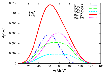
Figure 4: (Color online) ${}^{5}_{\Lambda}$He and ${}^{16}_{\Lambda}$O spectra: (a) without recoil, and (b) with recoil, evaluated within the IPSM for the P2 OME transition potential. Contributions of different orbitals $s_{1/2}$, $p_{3/2}$, and $p_{1/2}$ to the total ${}^{16}_{\Lambda}$O spectra are also displayed.

The energies ${E}_{\mbox{\tiny max}}$ are closely related to the liberated energies, i.e., to the ${Q}^{j}_{p}$-values since the latter should, in principle, also decrease when the $\Delta^{j}_{p}$ decrease. However, for light hypernuclei, this decrease is largely offset by the recoil effect, as shown by Eq. (20). The final results, displayed in Figs. 2 and 3, demonstrate that the Q-values are roughly constant and within the energy interval of $\sim 115-135$ MeV, which is consistent with the data within experimental errors.

Table 5: Results for the $\chi^{2}$ parameters $a$ and $b$, and the corresponding ratios ${\Gamma^{0}_{2}}/{\Gamma^{0}_{p}}$, and $\Gamma^{0}_{2}/\Gamma^{0}_{\rm NM}$ for FINUDA data [24], and different partition energies for ${\rm N}_{p}^{<}$, and ${\rm N}_{p}^{>}$: A) derived in Ref. [24] with ${E}^{\mbox{\tiny FINUDA}}_{\mbox{\tiny max}}$, B) and C) obtained here with ${E}^{\mbox{\tiny th}}_{\mbox{\tiny max}}$, and ${E}^{\mbox{\tiny th}}_{\mbox{\tiny even}}$, respectively.

case	$a$	$b$	${\Gamma^{0}_{2}}/{\Gamma^{0}_{p}}$	$\Gamma^{0}_{2}/\Gamma^{0}_{\rm NM}$
A	$0.654\pm 0.138$	$0.009\pm 0.013$	$0.43\pm 0.25$	$0.24\pm 0.10$
B	$0.711\pm 0.101$	$-0.010\pm 0.008$	$0.73\pm 0.61$	$0.33\pm 0.10$
C	$0.656\pm 0.101$	$-0.004\pm 0.008$	$0.45\pm 0.43$	$0.23\pm 0.09$

file=Fig4B1.eps,width=6cm

file=Fig4C1.eps,width=6cm

Figure 5: (Color online) Ratio $R$, given by (11) as a function of $A$ for the partition energies: (a) ${E}_{\mbox{\tiny max}}^{\mbox{\tiny th}}$, and (b) ${E}^{\mbox{\tiny th}}_{\mbox{\tiny even}}$.

In view of the differences between the FINUDA spectra and those calculated here, one is immediately tempted to repeat the above analysis using the energies ${E}^{\mbox{\tiny th}}_{\mbox{\tiny max}}$ instead of ${E}^{\mbox{\tiny FINUDA}}_{\mbox{\tiny max}}$. This was done and the results for $R$ are shown in the left panel of Figure 5, along with the corresponding linear $\chi^{2}$ fit. The large difference between the two sets of maxima gives rise to large differences between the values of the ratios $R$ in Ref. [24, Fig. 2] and those derived here. The parameters $a$ and $b$, and the ratios ${\Gamma^{0}_{2}}/{\Gamma^{0}_{p}}$, and $\Gamma^{0}_{2}/\Gamma^{0}_{\rm NM}$ obtained in this way are listed in row B of Table 5. The value of $a$ is not very different from the previous case but, as expected, $b$ is now negative, and the resulting $\Gamma^{0}_{2}$ is significantly different due to its strong sensitivity on $a$ in (32).

One must not forget here that, while the number of protons can be partitioned in many different ways, obtaining different results for the ratio defined in (28), the relations from (29) on are only valid when the condition $\Gamma_{p}^{0<}=\Gamma_{p}^{0>}=\Gamma^{0}_{p}/2$ is fulfilled, which does not occur for ${E}_{\mbox{\tiny max}}^{\mbox{\tiny th}}$. There is, however, always an energy ${E}^{\mbox{\tiny th}}_{\mbox{\tiny even}}$ for which this condition is fulfilled, and which are listed in the last column of Table 4. The values of new $R$, displayed in the lower panel of Fig. 5, are not very different from the previous values shown in the same figure. However, the value of the parameter $a$ and, consequently, the ratio ${\Gamma^{0}_{2}}/{\Gamma^{0}_{p}}$, is quite different now resembling those obtained by FINUDA, as can be seen from row C in Table 5. This agreement is somewhat surprising and we can not draw any conclusion from it. One has just learned that: (i) a relatively small modification of the partition energies (from ${E}_{\mbox{\tiny max}}^{\mbox{\tiny th}}$ to ${E}^{\mbox{\tiny th}}_{\mbox{\tiny even}}$) can lead to significantly different results for ${\Gamma^{0}_{2}}/{\Gamma^{0}_{p}}$, and (ii) a relatively sizeable modification of the partition energies (from ${E}_{\mbox{\tiny max}}^{\mbox{\tiny FINUDA}}$ to ${E}^{\mbox{\tiny th}}_{\mbox{\tiny even}}$) can lead to quite similar results for ${\Gamma_{2}^{0}}/{\Gamma^{0}_{p}}$.

It would be valuable to find the physical meaning of the fitting parameter $b$, which is different in the three cases discussed above. In this regard, how to arrive at (30) from (29) is not a trivial issue. One possibility is to neglect the last term in the denominator of (29), arguing, as was done in Ref. [24], that the FSIs tend to remove protons from the high energy part of the spectrum (${\rm N}_{FSI}^{>}<0$) while filling the low energy region (${\rm N}_{FSI}^{<}>0$), with the net result that ${\rm N}_{FSI}={\rm N}_{FSI}^{<}+{\rm N}_{FSI}^{>}\cong 0$. Therefore

$$R\cong a+\frac{{\rm N}_{FSI}^{<}}{(1+\Gamma^{0}_{2}/\Gamma^{0}_{p}){\rm N}_{p}^{0}},$$

which, when compared with (30), yields

$${{\rm N}_{FSI}^{<}}\cong b{A}{\rm N}_{p}^{0}\left(1+\frac{\Gamma_{2}^{0}}{\Gamma_{p}^{0}}\right)\sim b{A}{\rm N}_{p}^{0},$$ (33)

since the factor ${1+\Gamma^{0}_{2}/\Gamma^{0}_{p}}<1.5$ is unsubstantial for a qualitative discussion. At first glance, the last equation appears reasonable because the effect of the FSIs should increase with $A$. But, since $b=0.009\pm 0.013$, it turns out that ${\rm N}_{FSI}^{<}/{\rm N}_{p}^{0}\sim 0.01A$. Such a small amount of FSIs looks unrealistic. It is even more difficult to interpret physically the negative values of $b$ that we obtain in cases B and C. Evidently, the fact that the IPSM is unable to reproduce the low-energy spectra in no way affects the previous discussion of ${\Gamma^{0}_{2}}/{\Gamma^{0}_{p}}$.

A different derivation of the $2N$ branching ratio has been done at FINUDA quite recently [68], based on the analysis of the ($\pi^{-},p,n$) triple coincidence events, and a $\chi^{2}$ fit similar to (30). The new result, $\Gamma^{0}_{2}/\Gamma^{0}_{\rm NM}=021\pm 0.10$, is consistent within the errors with the previously obtained value [24], as well as with our result. Only the sum of events from all hypernuclear species are exhibited in this work, without presenting data for individual proton spectra, which would allow us to do a reanalysis similar to that done above.

6 Summary and Conclusions

Proton kinetic energy spectra of ${\mathrm{{}^{5}_{\Lambda}He}}$, ${\mathrm{{}^{7}_{\Lambda}Li}}$, ${\mathrm{{}^{9}_{\Lambda}Be}}$, ${\mathrm{{}^{11}_{\Lambda}B}}$, ${\mathrm{{}^{12}_{\Lambda}C}}$, ${\mathrm{{}^{13}_{\Lambda}C}}$, ${\mathrm{{}^{15}_{\Lambda}N}}$ and ${\mathrm{{}^{16}_{\Lambda}O}}$, measured by FINUDA a few years ago [24], were evaluated theoretically for the first time. We conclude that, in all the cases, the magnitudes of the spectra strongly depend on the parameterization that is used for the transition potential, while their shapes are very similar and independent of the transition mechanism. This statement, like all statements made in this work, do not depend at all on the inclusion or non-inclusion of the FSIs and $2N$-NM channel in the nuclear model.

It is explained in detail in Sec. 2 that our method for comparing the theory with experiment is radically different from the procedure followed by other researchers. In particular:

• The equations (4) have never been used so far by any other group. These relations show that, to evaluate the decay rates, it is essential to know the number of produced hypernuclei ${\rm N}_{W}$, which is not available in the literature.

• We focus our attention on measured transition probabilities $\Gamma_{N}$, and $\Gamma_{nN}$, instead of comparing bare quantities $\Gamma^{0}_{p}$, $\Gamma^{0}_{n}$, $\Gamma^{0}_{np}$, etc, which are extracted from the experiments by making assumptions and approximations that are often questionable.

• The difference with other studies can be immediately seen by facing our Eq. (14) with  [36, Eq. (7)].

• But, what is really important is that the method proposed here imposes more constraint in comparing theory with data, allowing us to examine more clearly the decay mechanism regardless of the importance of FSIs and the 2N-NM channel.

Despite the lack of direct information about the ${\rm N}_{W}$-values, we have been able to estimate these observables for ${\mathrm{{}^{5}_{\Lambda}He}}$, ${\mathrm{{}^{7}_{\Lambda}Li}}$, and ${\mathrm{{}^{12}_{\Lambda}C}}$ hypernuclei from the ratios $R_{p}$ presented in Ref. [22]. (The physical meaning of this ratio is also clarified.) In this way, we obtain in Sec. 3 some very useful information on the transition potential. In fact, from Figs. 2 and 3 and Table 1, we conclude that:

• The IPSM reproduces correctly the shapes of all proton kinetic energy spectra $S_{p}(E_{p})$ at medium and high energies ($E_{p}\>\raisebox{-2.15277pt}{$\stackrel{{\scriptstyle\textstyle>}}{{\sim}}$}\>40$ MeV), including the $Q$-value, which is around $115-135$ MeV. The latter could indicate that the residual nucleus ${}^{A-2}(Z-1)$ is emitted mainly in the ground state.

• This simple model also reproduces fairly well the magnitudes of the spectra at these energies when the soft $\pi+K$ potential is used to describe the NMWD. In no way do we claim that this is the ”true” physics, but we believe that it might be worth pursuing this direction, especially considering that the model is able to explain satisfactorily the NM decay rates $\Gamma_{p}$ and $\Gamma_{n}$ of the s-shell hypernuclei [8, 9].

• The measured transition rates, $\Gamma_{p}$, the same as the corresponding spectral densities $S_{p}(E_{p})$ for $E_{p}\>\raisebox{-2.15277pt}{$\stackrel{{\scriptstyle\textstyle>}}{{\sim}}$}\>40$ MeV, are significantly overestimated by the present theoretical calculations when the standard parametrization for the transition potential is used. In doing this comparison, one should keep in mind that, while the calculations refer to the $1N$-NM decay mode only, the measured rates include also the $2N$-NM decay channel and the effects of FSIs, and therefore the latter should always be larger. This happens only for the soft $\pi+K$ exchange potential.

• It is difficult to reconcile the FINUDA data with the theory based on the $\pi+2\pi/\rho+2\pi/\sigma+\omega+K+\rho\pi/a_{1}+\sigma\pi/a_{1}$ exchange potential [17].

We strongly believe that, in recent theoretical calculations [36, 38], which include both the $2N$-NM decay channel, and the FSIs, they would have arrived at very similar conclusions if the comparison with experimental data have been made ​​in the manner proposed here.

Since the calculated spectra only involve the $1N$-NM channel, the differences between them and the experimental spectra, both with respect to the magnitude and in relation to the energy distribution, can indicate which other degrees of freedom are important ($2N$-NM channel, FSIs, etc ). Our plan of action is to add them to $1N$-NM, when necessary, in order to successfully reproduce the experiments.

With regard to the FINUDA method [24] to determine the $2N$-NM decay rate, based on the assumption that the $1N$-NM strength of the kinetic proton spectra is equally distributed in the low and high energies, we conclude that:

• The proposed method is very sensitive to the energies that separate these two regions, and these energies can not be determined experimentally.

• The separation done in Ref. [24] is not supported by any firm physical argument.

• It is necessary to resort to theoretical models to establish the partition energies; the IPSM is very suitable for this purpose.

• Both theoretical sets of partition energies (${E}^{\mbox{\tiny th}}_{\mbox{\tiny max}}$, ${E}^{\mbox{\tiny th}}_{\mbox{\tiny even}}$) differ from the FINUDA result (${E}^{\mbox{\tiny FINUDA}}_{\mbox{\tiny max}}$), not only in magnitudes but also with regards to the mass-number dependence: ${E}^{\mbox{\tiny th}}_{\mbox{\tiny max}}$ and ${E}^{\mbox{\tiny th}}_{\mbox{\tiny even}}$ decrease with $A$, because the experimental single-particle energies increase; meanwhile, no reasonable explanation exists for the opposite behavior of ${E}^{\mbox{\tiny FINUDA}}_{\mbox{\tiny max}}$.

• In spite of the above mentioned differences, all three sets of partition energies yield similar results for the parameter $a$ and therefore for the ratio $\Gamma^{0}_{2}/\Gamma^{0}_{p}$. This indicates that the behavior with $A$ of the partition energies does not play a crucial role, and is consistent with a recent proposal to approximate them by a rather constant value of $\>\raisebox{-2.15277pt}{$\stackrel{{\scriptstyle\textstyle<}}{{\sim}}$}\>80$ MeV  [67].

• Physical interpretation of the FINUDA parameter $b$ is a point at issue, not only for being very small, but also because it is negative in our analysis, as well as in the a new study [68] of the contribution of the $2N$-NM channel employing the same method. Although suffering from large errors, its small value inevitably leads to the conclusion that the FSIs are very small, and that, therefore, the low-energy proton spectra dominantly comes from the $2N$-NM decay. It is very hard to understand this fact, and the only alternative possibility is that the basic approach (30) was incorrect.

Final remarks:

1. As stated in the beginning, our purpose was not to reproduce the experimental data, but to discover out what the proton kinetic energy spectra can tell us about the weak hypernuclear interaction. To account for the low energy data of the kinetic energy spectra, it is imperative to consider the FSIs. For the time being, we are working on this issue by employing an improved version of the CRISP internuclear cascade model [69] used previously to describe ${\mathrm{{}^{12}_{\Lambda}C}}$ [43, 44].

   Moreover, a complete theoretical description must also include a judicious estimate of the effect of the $2N$-NM decay channel. So far, this has been done only in the context of FGM [36, 38], and it would be interesting to know what the SM can tell us about this process. In fact, for quite some time, we have been involved in the development of a corresponding theoretical formalism and numerical codes [70].

2. To study the FSIs and the $2N$-NM decay, it is indispensable to understand first the $1N$-NM-decay dynamics. In our opinion, the SM could be a very useful tool to achieve this goal. For instance, the SM spectra are the main ingredients for establishing the initial conditions for the FSIs within the many-body multi-collision Monte Carlo cascade scheme [43, 44]. On the other hand, from Fig. 1, it is self-evident that the diagram a) plays the principal role within the diagram b) representing the $2N$-NM decay mode.

3. New experimental developments will be very welcome, such as: i) Angular correlation of $np$ and $nn$ pairs to determine the $\Gamma_{np}$ and $\Gamma_{nn}$ rates, which have been measured so far only by KEK [34] in ${}_{\Lambda}^{12}$C, and ii) Triple $(p,n,n)$, and $(p,p,n)$ coincidence detections for direct measurement of $\Gamma_{pn}$, and $\Gamma_{pp}$, as suggested previously [65]. The first steps in this direction seems to be given recently in Ref. [67].

4. To complete Figs. 2 and 3, we need the ${\rm N}_{W}$-values for ${\mathrm{{}^{9}_{\Lambda}Be}}$, ${\mathrm{{}^{11}_{\Lambda}B}}$, ${\mathrm{{}^{13}_{\Lambda}C}}$, ${\mathrm{{}^{15}_{\Lambda}N}}$ and ${\mathrm{{}^{16}_{\Lambda}O}}$ hypernuclei. Hopefully, these numbers will soon be available for public use.​ Needless to point out that, otherwise, the proton kinetic energy spectra measured by FINUDA [24] are of little use to study the NMWD dynamics. They only can be exploited to discuss the decay kinematics through the analysis of the FSIs and the $2N$-NM decay mode.

References

- [1] W.M. Alberico, G. Garbarino, Phys. Rep. 369, (2002) 1.
- [2] V. G. J. Stoks, R. A. M. Klomp, C. P. F. Terheggen, and J. J. de Swart, Phys. Rev. C 49, (1994) 2950.
- [3] J. F. Dubach, G. B. Feldman, B. R. Holstein, L. de la Torre, Ann. Phys. (N.Y.) 249, (1996) 146.
- [4] A. Parreño, A. Ramos, and C. Bennhold, Phys. Rev. C 56, (1997) 339.
- [5] R. Bockmann, C. Hanhart, O. Krehl, S. Krewald, and J. Speth, Phys. Rev. C 60, (1999) 055212.
- [6] K. Nakayama, privite comunication (2012).
- [7] J. Ryckebusch, M. Vanderhaeghen, L. Machenil, and M. Waroquier, Nucl. Phys. A 568, (1994) 828.
- [8] E. Bauer, A.P. Galeão, M. Hussein, F. Krmpotić, and J.D. Parker, Phys. Lett. B 674, (2009) 103.
- [9] F. Krmpotić, Few-Body Syst 55, (2014) 219.
- [10] F. Krmpotić, Phys. Rev. C 82, (2010) 055204.
- [11] A. Parreño, A. Ramos, Phys. Rev. C 65, (2001) 015204.
- [12] K. Sasaki, T. Inoue, and M. Oka, Nucl.Phys. A 669, (2000) 331; Erratum-ibid. A 678, (2000) 455.
- [13] K. Sasaki, T. Inoue, and M. Oka, Nucl. Phys. A 707, (2002) 477.
- [14] A. Parreño, C Bennhold, and B. R. Holstein, Phys. Rev. C 70, (2004) 051601.
- [15] C. Chumillas, G. Garbarino, A. Parreño, and A. Ramos, Phys. Lett. B 657, (2007) 180.
- [16] K. Itonaga, T. Motoba, T. Ueda, and Th.A. Rijken, Phys. Rev. C 77, (2008) 044605.
- [17] K. Itonaga, T. Motoba, Prog. Theor. Phys. Suppl. 185, (2010) 252.
- [18] M. Ruderman and R. Karplus, Phys. Rev. 102, (1956) 247.
- [19] W.M. Alberico, A. De Pace, M. Ericson, and A. Molinar, Phys. Lett. B 256, (1991) 134.
- [20] A. Ramos, E. Oset and L.L. Salcedo, Phys. Rev. C 50, (1994) 2314.
- [21] M. J. Kim, et al., Phys. Rev. Lett. 103, (2009) 182502 .
- [22] M. Agnello et al., Nucl. Phys. A 804, (2008) 151.
- [23] M. Agnello et al., Phys. Lett. B 681, (2009) 139.
- [24] M. Agnello et al., Phys. Lett. B 685, (2010) 247.
- [25] E. Bauer, and G. Garbarino, Nucl. Phys. A 828, (2009) 29.
- [26] J. D. Parker et al., Phys. Rev. C 76, (2007) 035501.
- [27] J.J. Szymanski et al., Phys. Rev. C 43, (1991) 849.
- [28] H. Noumi et al., Phys. Rev. C 52, (1995) 2936.
- [29] J. H. Kim et al., Phys. Rev. C 68, (2003) 065201.
- [30] S. Okada et al., Phys. Lett. B 597, (2004) 249.
- [31] S. Okada et al., Nucl. Phys. A 752 , (2005) 196.
- [32] H. Outa et al., Nucl. Phys. A 754 , (2005) 157c.
- [33] B. H. Kang et al., Phys. Rev. Lett. 96, (2006) 062301.
- [34] M. J. Kim et al., Phys. Lett. B 641, (2006) 28.
- [35] H. Bhang et al., Eur. Phys. J. A 33, (2007) 259.
- [36] E. Bauer, G. Garbarino, A. Parreño, and A. Ramos, Nucl. Phys. A 836, (2010) 199.
- [37] E. Bauer, and G. Garbarino, Phys. Rev. C 81, (2010) 064315.
- [38] E. Bauer, and G. Garbarino, Phys. Lett. B 698, (2011) 306.
- [39] O. Benhar, Nucl. Phys. B (Proc. Suppl.) 159, (2006) 168.
- [40] A. Meucci, C. Giusti, M. Vorabbi, Phys. Rev. D 88 013006.
- [41] H. F. Schopper , Weak Interactions and Nuclear -decay (North-Holland Publ. Co., Amsterdam, 1966).
- [42] A. Ramos, M. J. Vicente-Vacas, and E. Oset, Phys. Rev. C 55, 735 (1997);C 66, 039903 (2002)(E).
- [43] I. Gonzalez et al., J. Phys. Conf. Ser. 312, (2011) 022017.
- [44] I. Gonzalez, C. Barbero, A. Deppman, S. Duarte, F. Krmpotić, O. Rodriguez, J. Phys. G: Nucl. Part. Phys. 38, (2011) 115105.
- [45] A. Deppman, S. B. Duarte, G. Silva, O. A. P. Tavares, S. Anefalos, J. D. T. Arruda-Neto, T. Rodrigues J. Phys. G: Nucl. Part. Phys. 30 1991.
- [46] A. Deppman, G. Silva, S. Anefalos, S. B. Duarte, F. Garcia, F. H. Hisamoto, O. A. P. Tavares Phys. Rev. C 73 064607.
- [47] A. Deppman, O. A. P. Tavares , S. B. Duarte, E. C. Oliveira, J. D. T. Arruda-Neto, S. de Pina, V. Likhachev, O. Rodriguez, J. Mesa, M. Gonçalves Phys. Rev. Lett. 87 82701
- [48] O. A. P. Tavares , S. B. Duarte, V. Likhachev, A. Deppman J. Phys. G: Nucl. Part. Phys. 30 37.
- [49] G. Garbarino, A. Parreño, and A. Ramos, Phys. Rev. C 69, (2004) 054603.
- [50] E. Botta,Weak Decay of Hypernuclei (FINUDA, KEK) – Experiment, SPHERE School + 22nd Indian-Summer School of Physics STRANGENESS NUCLEAR PHYSICS, Rez/Prague, Czech Republic (2010).
- [51] D. P. Heddle and L.S . Kisslinger, Phys. Rev. C 33, (1986) 608.
- [52] J. Cohen, Prog. Part. Nucl. Phys. 25, (1990) 139.
- [53] C. Barbero, D. Horvat, F. Krmpotić, T. T. S. Kuo, Z. Narančić, and D. Tadić, Phys. Rev. C 66, (2002) 055209.
- [54] F. Krmpotić, and D. Tadić, Braz. J. Phys. 33, (2003) 187.
- [55] C. Barbero, C. De Conti, A. P. Galeão and F. Krmpotić, Nucl. Phys. A 726, (2003) 267.
- [56] C. Barbero, A. P. Galeão, and F. Krmpotić, Phys. Rev. C 76, (2007) 054321.
- [57] C. Barbero, A. P. Galeão, M. S. Hussein, and F. Krmpotić, Phys. Rev. C 78, (2008) 044312; Erratum-ibid. 059901(E).
- [58] E. Bauer, A. P. Galeão, M. S. Hussein and F. Krmpotić, Nucl. Phys. A 834, (2010) 599c.
- [59] F. Krmpotić, A. P. Galeão, and M.S. Hussein, AIP Conf. Proc. 1245, (2010) 51.
- [60] F. Krmpotić, A. Samana, and A. Mariano, Phys. Rev. C 71, (2005) 044319 .
- [61] E. Bauer, Nucl. Phys. A 818, (2009) 174.
- [62] TUNL Nuclear Data Project, www.tunl.duke.edu/nucldata/ (2012).
- [63] D.J. Millener, Lecture Notes in Physics 724 (Springer, 2007) 31.
- [64] G. Garbarino, A. Parreño and A. Ramos, Phys. Rev. Lett. 91, (2003) 112501.
- [65] C. de Conti, A. Deppman, F. Krmpotić, arXiv:1202.4223.
- [66] G. Jacob and T. A. J. Maris, Rev. Mod. Phys. 45, (1973) 6.
- [67] S. Bufalino, Nucl. Phys. A 914, (2013) 160.
- [68] M. Agnello et al., Phys. Lett. B 701, (2011) 556.
- [69] C. Barbero, A. Deppman, S. Duarte, F. Krmpotić, in preparation.
- [70] C. Barbero, E. Bauer, C. De Conti, A. P. Galeão and F. Krmpotić, in preparation.