Sparse Bayesian Dictionary Learning with a Gaussian Hierarchical Model

Abstract

We consider a dictionary learning problem whose objective is to design a dictionary such that the signals admits a sparse or an approximate sparse representation over the learned dictionary. Such a problem finds a variety of applications such as image denoising, feature extraction, etc. In this paper, we propose a new hierarchical Bayesian model for dictionary learning, in which a Gaussian-inverse Gamma hierarchical prior is used to promote the sparsity of the representation. Suitable priors are also placed on the dictionary and the noise variance such that they can be reasonably inferred from the data. Based on the hierarchical model, a variational Bayesian method and a Gibbs sampling method are developed for Bayesian inference. The proposed methods have the advantage that they do not require the knowledge of the noise variance a priori. Numerical results show that the proposed methods are able to learn the dictionary with an accuracy better than existing methods, particularly for the case where there is a limited number of training signals.

I Introduction

Sparse representation has been of significant interest over past few years and has found a variety of applications in practice as many natural signals admit a sparse or an approximate sparse representation in a certain basis [1, 2, 3]. In many applications such as image denoising and interpolation, signals are assumed to admit a sparse representation over a pre-specified non-adaptive dictionary, e.g. discrete consine/wavelet transform (DCT/DWT) bases. Nevertheless, recent research [4, 5] has shown that the recovery, denoising and classification performance can be considerably improved by utilizing an adaptive dictionary that is learned from the training signals [5, 6]. This has inspired studies on dictionary learning whose objective is to design overcompelete dictionaries that can better represent the signals. A number of algorithms, such as K-singular value decomposition (K-SVD) [4], method of optimal directions (MOD) [7], dictionary learning with the majorization method [8], and simultaneous codeword optimization (SimCO) [9], were developed for learning overcomplete dictionaries for sparse representation. Most algorithms formulate the dictionary learning as an optimization problem and solve it via a two-stage iterative process, namely, a sparse coding stage and a dictionary update stage. The main difference between these algorithms lies in the dictionary update stage. Specifically, the MOD method [7] updates the dictionary via solving a least square problem which admits a closed-form for the dictionary update. The K-SVD algorithm [4], instead, updates atoms of the dictionary in a sequential manner and while updating each atom, the atom is updated along with the nonzero entries in the corresponding row vector of the sparse matrix. The idea of this sequential atom update was later extended to sequentially updating multiple atoms each time [9], and recently was generalized to parallel atom-updating in order to further accelerate the convergence of the iterative process [10]. These methods [4, 7, 8, 9, 10], although delivering state-of-the-art performance, require the knowledge of the sparsity level or the noise/residual variance to define the stopping criterion for estimating the sparse codes (e.g. [4]), or select appropriate values for the regularization parameters controlling the tradeoff between the sparsity level and the data fitting error (e.g. [8, 10]). In practice, however, the prior information about the noise variance is usually unavailable and an inaccurate estimation may result in substantial performance degradation. To mitigate this limitation, a nonparametric Bayesian dictionary learning method called as beta-Bernoulli process factor analysis (BPFA) was recently developed in [11]. The proposed method is able to automatically infer the required number of factors (dictionary elements) and the noise variance from the image under test, which is deemed as an important advantage over other dictionary learning methods. For [11], the posterior distributions cannot be derived analytically, and a Gibbs sampler was used for Bayesian inference. We also note that a class of online dictionary learning algorithms were developed in [12, 13, 14]. Different from the above batch-based algorithms [4, 7, 9, 10] which use the whole set of training data for dictionary learning, online algorithms continuously update the dictionary using only one or a small batch of training data, which enables them to handle very large data sets.

In this paper, we propose a new hierarchical Bayesian model for dictionary learning, in which a Gaussian-inverse Gamma hierarchical prior is used to promote the sparsity of the representation. Suitable priors are also placed on the dictionary and the noise variance such that they can be reasonably inferred from the data. Based on the hierarchical model, a variational Bayesian method and a Gibbs sampling method are developed for Bayesian inference. For both inference methods, there are two different ways to update the dictionary: we can update the whole set of atoms at once, or update the atoms in a sequential manner. When updating the dictionary as a whole, the proposed variational Bayesian method has a dictionary update formula similar to the MOD method. Nevertheless, unlike the MOD method which alternates between two separate stages (i.e. dictionary update and sparse coding), for our algorithm, the dictionary and the signal are refined in an interweaved and gradual manner, which enables the algorithm to come to a reasonably nearby point as the optimization progresses, and helps avoid undesirable local minima. For the Gibbs sampler, a sequential update seems able to expedite the convergence rate and helps achieve better performance. Simulation results show that the proposed Gibbs sampling algorithm presents uniform superiority over other state-of-the-art dictionary learning methods in a number of experiments.

The rest of the paper is organized as follows. In Section II, we introduce a hierarchical prior model for learning dictionaries. Based on this hierarchical model, a variational Bayesian method and a Gibbs sampler are developed in Section III and Section IV for Bayesian inference. Simulation results are provided in Section V, followed by concluding remarks in Section VI.

II Hierarchical Model

Suppose we have $L$ training signals $\{\boldsymbol{y}_{l}\}_{l=1}^{L}$, where $\boldsymbol{y}_{l}\in\mathbb{R}^{M}$. Dictionary learning aims at finding a common sparsifying dictionary $\boldsymbol{D}\in\mathbb{R}^{M\times N}$ such that these $L$ training signals admit a sparse representation over the overcomplete dictionary $\boldsymbol{D}$, i.e.

$$\boldsymbol{y}_{l}=\boldsymbol{D}\boldsymbol{x}_{l}+\boldsymbol{w}_{l}\qquad\forall l$$ (1)

where $\boldsymbol{x}_{l}$ and $\boldsymbol{w}_{l}$ denote the sparse vector and the residual/noise vector, respectively. Define $\boldsymbol{Y}\triangleq[\boldsymbol{y}_{1}\phantom{0}\ldots\phantom{0}\boldsymbol{y}_{L}]$, $\boldsymbol{X}\triangleq[\boldsymbol{x}_{1}\phantom{0}\ldots\phantom{0}\boldsymbol{x}_{L}]$, and $\boldsymbol{W}\triangleq[\boldsymbol{w}_{1}\phantom{0}\ldots\phantom{0}\boldsymbol{w}_{L}]$, the model (1) can be re-expressed as

$$\boldsymbol{Y}=\boldsymbol{D}\boldsymbol{X}+\boldsymbol{W}$$ (2)

Also, we write $\boldsymbol{D}\triangleq[\boldsymbol{d}_{1}\phantom{0}\ldots\phantom{0}\boldsymbol{d}_{N}]$, where each column of the dictionary, $\boldsymbol{d}_{n}$, is called an atom.

In the following, we develop a Bayesian framework for learning the overcomplete dictionary and sparse vectors. To promote sparse representations, we assign a two-layer hierarchical Gaussian-inverse Gamma prior to $\boldsymbol{X}$. The Gaussian-inverse Gamma prior is one of the most popular sparse-promoting priors which has been widely used in compressed sensing [15, 16, 17]. In the first layer, $\boldsymbol{X}$ is assigned a Gaussian prior distribution

$$p(\boldsymbol{X}|\boldsymbol{\alpha})= \prod_{n=1}^{N}\prod_{l=1}^{L}p(x_{nl})$$

$$= \prod_{n=1}^{N}\prod_{l=1}^{L}\mathcal{N}(x_{nl}|0,\alpha_{nl}^{-1})$$ (3)

where $x_{nl}$ denotes the $(n,l)$th entry of $\boldsymbol{X}$, and $\boldsymbol{\alpha}\triangleq\{\alpha_{nl}\}$ are non-negative sparsity-controlling hyperparameters. The second layer specifies Gamma distributions as hyperpriors over the hyperparameters $\{\alpha_{nl}\}$, i.e.

$$p(\boldsymbol{\alpha})= \prod_{n=1}^{N}\prod_{l=1}^{L}\text{Gamma}(\alpha_{nl}|a,b)$$

$$= \prod_{n=1}^{N}\prod_{l=1}^{L}\Gamma(a)^{-1}b^{a}\alpha_{nl}^{a-1}e^{-b\alpha_{nl}}$$ (4)

where $\Gamma(a)=\int_{0}^{\infty}t^{a-1}e^{-t}dt$ is the Gamma function, and the parameters $a$ and $b$ used to characterize the Gamma distribution are usually chosen to be small values, e.g. $10^{-6}$. As discussed in [18], this hyperprior allows the posterior mean of $\alpha_{nl}$ to become arbitrarily large. As a consequence, the associated coefficient $x_{nl}$ will be driven to zero, thus yielding a sparse solution. In this paper, we choose a value of $a=0.5$ in order to achieve a more sparsity-encouraging effect. Clearly, the Gamma prior with a larger $a$ encourages large values of the hyperparameters, and therefore promotes the sparseness of the solution since the larger the hyperparameter, the smaller the variance of the corresponding coefficient.

In addition, in order to prevent the dictionary from becoming infinitely large, we assume the atoms of the dictionary $\{\boldsymbol{d}_{n}\}$ are mutually independent and each atom is placed a Gaussian prior, i.e.

$$p(\boldsymbol{D})=\prod_{n=1}^{N}p(\boldsymbol{d}_{n})=\prod_{n=1}^{N}\mathcal{N}(\boldsymbol{d}_{n}|\boldsymbol{0},\beta\boldsymbol{I})$$ (5)

where $\beta$ is a parameter whose choice will be discussed later. The noise $\{\boldsymbol{w}_{l}\}$ are assumed independent multivariate Gaussian noise with zero mean and covariance matrix $(1/\gamma)\boldsymbol{I}$, where the noise variance $1/\gamma$ is assumed unknown a priori. To estimate the noise variance, we place a Gamma hyperprior over $\gamma$, i.e.

$$p(\gamma)=\text{Gamma}(\gamma|c,d)=\Gamma(c)^{-1}d^{c}\gamma^{c-1}e^{-d\gamma}$$ (6)

where we set $c=0.5$ and $d=10^{-6}$. The proposed hierarchical model (see Fig. 1) provides a general framework for learning the overcomplete dictionary, the sparse codes, as well as the noise variance. In the following, we will develop a variational Beyesian method and a Gibbs sampling method for Bayesian inference.

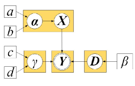
Figure 1: Hierarchical model for dictionary learning.

III Variational Inference

III-A Review of The Variational Bayesian Methodology

Before proceeding, we firstly provide a brief review of the variational Bayesian methodology. In a probabilistic model, let $\boldsymbol{y}$ and $\boldsymbol{\theta}$ denote the observed data and the hidden variables, respectively. It is straightforward to show that the marginal probability of the observed data can be decomposed into two terms

$$\ln p(\boldsymbol{y})=L(q)+\text{KL}(q||p)$$ (7)

where

$$L(q)=\int q(\boldsymbol{\theta})\ln\frac{p(\boldsymbol{y},\boldsymbol{\theta})}{q(\boldsymbol{\theta})}d\boldsymbol{\theta}$$ (8)

and

$$\text{KL}(q||p)=-\int q(\boldsymbol{\theta})\ln\frac{p(\boldsymbol{\theta}|\boldsymbol{y})}{q(\boldsymbol{\theta})}d\boldsymbol{\theta}$$ (9)

where $q(\boldsymbol{\theta})$ is any probability density function, $\text{KL}(q||p)$ is the Kullback-Leibler divergence between $p(\boldsymbol{\theta}|\boldsymbol{y})$ and $q(\boldsymbol{\theta})$. Since $\text{KL}(q||p)\geq 0$, it follows that $L(q)$ is a rigorous lower bound on $\ln p(\boldsymbol{y})$. Moreover, notice that the left hand side of (7) is independent of $q(\boldsymbol{\theta})$. Therefore maximizing $L(q)$ is equivalent to minimizing $\text{KL}(q||p)$, and thus the posterior distribution $p(\boldsymbol{\theta}|\boldsymbol{y})$ can be approximated by $q(\boldsymbol{\theta})$ through maximizing $L(q)$.

The significance of the above transformation is that it circumvents the difficulty of computing the posterior probability $p(\boldsymbol{\theta}|\boldsymbol{y})$ (which is usually computationally intractable). For a suitable choice for the distribution $q(\boldsymbol{\theta})$, the quantity $L(q)$ may be more amiable to compute. Specifically, we could assume some specific parameterized functional form for $q(\boldsymbol{\theta})$ and then maximize $L(q)$ with respect to the parameters of the distribution. A particular form of $q(\boldsymbol{\theta})$ that has been widely used with great success is the factorized form over the component variables $\{\theta_{i}\}$ in $\boldsymbol{\theta}$ [19], i.e. $q(\boldsymbol{\theta})=\prod_{i}q_{i}(\theta_{i})$. We therefore can compute the posterior distribution approximation by finding $q(\boldsymbol{\theta})$ of the factorized form that maximizes the lower bound $L(q)$. The maximization can be conducted in an alternating fashion for each latent variable, which leads to [19]

$$q_{i}(\theta_{i})=\frac{\exp(\langle\ln p(\boldsymbol{y},\boldsymbol{\theta})\rangle_{k\neq i})}{\int\exp(\langle\ln p(\boldsymbol{t},\boldsymbol{\theta})\rangle_{k\neq i})d\theta_{i}}$$ (10)

where $\langle\cdot\rangle_{k\neq i}$ denotes an expectation with respect to the distributions $q_{i}(\theta_{i})$ for all $k\neq i$.

III-B Proposed Variational Bayesian Method

We now proceed to perform variational Bayesian inference for the proposed hierarchical model. Let $\boldsymbol{\theta}\triangleq\{\boldsymbol{X},\boldsymbol{\alpha},\boldsymbol{D},\gamma\}$ denote all hidden variables. We assume posterior independence among the variables $\boldsymbol{X}$, $\boldsymbol{\alpha}$, $\boldsymbol{D}$ and $\gamma$, i.e.

$$p(\boldsymbol{\theta}|\boldsymbol{y})\approx q(\boldsymbol{x},\boldsymbol{\alpha},\boldsymbol{D},\gamma)$$

$$= q_{x}(\boldsymbol{x})q_{\alpha}(\boldsymbol{\alpha})q_{d}(\boldsymbol{D})q_{\gamma}(\gamma)$$ (11)

With this mean field approximation, the posterior distribution of each hidden variable can be computed by maximizing $L(q)$ while keeping other variables fixed using their most recent distributions, which gives

$$\ln q_{x}(\boldsymbol{X})= \langle\ln p(\boldsymbol{Y},\boldsymbol{X},\boldsymbol{D},\boldsymbol{\alpha},\gamma)\rangle_{q_{d}(\boldsymbol{D})q_{\alpha}(\boldsymbol{\alpha})q_{\gamma}(\gamma)}+\text{constant}$$

$$\ln q_{d}(\boldsymbol{D})= \langle\ln p(\boldsymbol{Y},\boldsymbol{X},\boldsymbol{D},\boldsymbol{\alpha},\gamma)\rangle_{q_{x}(\boldsymbol{X})q_{\alpha}(\boldsymbol{\alpha})q_{\gamma}(\gamma)}+\text{constant}$$

$$\ln q_{\alpha}(\boldsymbol{\alpha})= \langle\ln p(\boldsymbol{Y},\boldsymbol{X},\boldsymbol{D},\boldsymbol{\alpha},\gamma)\rangle_{q_{x}(\boldsymbol{X})q_{d}(\boldsymbol{D})q_{\gamma}(\gamma)}+\text{constant}$$

$$\ln q_{\gamma}(\gamma)= \langle\ln p(\boldsymbol{Y},\boldsymbol{X},\boldsymbol{D},\boldsymbol{\alpha},\gamma)\rangle_{q_{x}(\boldsymbol{X})q_{d}(\boldsymbol{D})q_{\alpha}(\boldsymbol{\alpha})}+\text{constant}$$

where $\langle\rangle_{q_{1}(\cdot)\ldots q_{K}(\cdot)}$ denotes the expectation with respect to (w.r.t.) the distributions $\{q_{k}(\cdot)\}_{k=1}^{K}$. In summary, the posterior distribution approximations are computed in an alternating fashion for each hidden variable, with other variables fixed. Details of this Bayesian inference scheme are provided below.

1). Update of $q_{x}(\boldsymbol{X})$: The calculation of $q_{x}(\boldsymbol{X})$ can be decomposed into a set of independent tasks, with each task computing the posterior distribution approximation for each column of $\boldsymbol{X}$, i.e. $q_{x}(\boldsymbol{x}_{l})$. We have

$$\ln q_{x}(\boldsymbol{x}_{l})\propto \langle\ln[p(\boldsymbol{y}_{l}|\boldsymbol{D},\boldsymbol{x}_{l},\gamma)p(\boldsymbol{x}_{l}|\boldsymbol{\alpha}_{l})]\rangle_{q_{d}(\boldsymbol{D})q_{\alpha}(\boldsymbol{\alpha})q_{\gamma}(\gamma)}$$ (12)

where $\boldsymbol{\alpha}_{l}\triangleq\{\alpha_{nl}\}_{n=1}^{N}$ is the sparsity-controlling hyperparameters associated with $\boldsymbol{x}_{l}$, $p(\boldsymbol{y}_{l}|\boldsymbol{D},\boldsymbol{x}_{l},\gamma)$ and $p(\boldsymbol{x}_{l}|\boldsymbol{\alpha}_{l})$ are respectively given by

$$p(\boldsymbol{y}_{l}|\boldsymbol{D},\boldsymbol{x}_{l},\gamma)= \left(\frac{\gamma}{2\pi}\right)^{\frac{M}{2}}\exp\left(-\frac{\gamma\|\boldsymbol{y}_{l}-\boldsymbol{D}\boldsymbol{x}_{l}\|_{2}^{2}}{2}\right)$$

$$p(\boldsymbol{x}_{l}|\boldsymbol{\alpha}_{l})= \prod_{n=1}^{N}\mathcal{N}(x_{nl}|0,\alpha_{nl}^{-1})$$ (13)

Substituting (13) into (12) and after some simplifications, it can be readily verified that $q_{x}(\boldsymbol{x}_{l})$ follows a Gaussian distribution

$$q_{x}(\boldsymbol{x}_{l})=\mathcal{N}(\boldsymbol{x}_{l}|\boldsymbol{\mu}_{l}^{x},\boldsymbol{\Sigma}_{l}^{x})$$ (14)

with its mean $\boldsymbol{\mu}_{l}^{x}$ and covariance matrix $\boldsymbol{\Sigma}_{l}^{x}$ given respectively as

$$\boldsymbol{\mu}_{l}^{x}= \langle\gamma\rangle\boldsymbol{\Sigma}_{l}^{x}\langle\boldsymbol{D}\rangle^{T}\boldsymbol{y}_{l}$$

$$\boldsymbol{\Sigma}_{l}^{x}= \left(\langle\gamma\rangle\langle\boldsymbol{D}^{T}\boldsymbol{D}\rangle+\langle\boldsymbol{\Lambda}_{l}\rangle\right)^{-1}$$ (15)

where $\langle\gamma\rangle$ denotes the expectation w.r.t. $q_{\gamma}(\gamma)$, $\langle\boldsymbol{D}\rangle$ and $\langle\boldsymbol{D}^{T}\boldsymbol{D}\rangle$ denote the expectation w.r.t. $q_{d}(\boldsymbol{D})$, and $\langle\boldsymbol{\Lambda}_{l}\rangle\triangleq\text{diag}(\langle\alpha_{1l}\rangle,\ldots,\langle\alpha_{Nl}\rangle)$, in which $\langle\alpha_{nl}\rangle$ represents the expectation w.r.t. $q_{\alpha}(\boldsymbol{\alpha})$.

2). Update of $q_{d}(\boldsymbol{D})$: The approximate posterior $q_{d}(\boldsymbol{D})$ can be obtained as

$$\ln q_{d}(\boldsymbol{D})\propto \langle\ln[p(\boldsymbol{Y}|\boldsymbol{X},\boldsymbol{D},\gamma)p(\boldsymbol{D})]\rangle_{q_{x}(\boldsymbol{X})q_{\gamma}(\gamma)}$$

$$\propto \langle-\gamma\|\boldsymbol{Y}-\boldsymbol{D}\boldsymbol{X}\|_{F}^{2}-\beta^{-1}\sum_{n=1}^{N}\boldsymbol{d}_{n}^{T}\boldsymbol{d}_{n}\rangle$$

$$\propto \langle-\gamma\text{tr}\{(\boldsymbol{Y}-\boldsymbol{D}\boldsymbol{X})(\boldsymbol{Y}-\boldsymbol{D}\boldsymbol{X})^{T}\}-\beta^{-1}\text{tr}\{\boldsymbol{D}\boldsymbol{D}^{T}\}\rangle$$

$$\propto \langle\text{tr}\{\boldsymbol{D}(\gamma\boldsymbol{X}\boldsymbol{X}^{T}+\beta^{-1}\boldsymbol{I})\boldsymbol{D}^{T}-2\gamma\boldsymbol{Y}\boldsymbol{X}^{T}\boldsymbol{D}^{T}\}\rangle$$

$$= \text{tr}\{\boldsymbol{D}(\langle\gamma\rangle\langle\boldsymbol{X}\boldsymbol{X}^{T}\rangle+\beta^{-1}\boldsymbol{I})\boldsymbol{D}^{T}-2\langle\gamma\rangle\boldsymbol{Y}\langle\boldsymbol{X}\rangle^{T}\boldsymbol{D}^{T}\}$$ (16)

where for simplicity, we have dropped the subscript of the $\langle\cdot\rangle$ operator. Define

$$\boldsymbol{A}\triangleq (\langle\gamma\rangle\langle\boldsymbol{X}\boldsymbol{X}^{T}\rangle+\beta^{-1}\boldsymbol{I})^{-1}$$

$$\boldsymbol{B}\triangleq \langle\gamma\rangle\boldsymbol{Y}\langle\boldsymbol{X}\rangle^{T}$$

The posterior $q_{d}(\boldsymbol{D})$ can be further expressed as

$$\ln q_{d}(\boldsymbol{D})\propto \text{tr}\{\boldsymbol{D}\boldsymbol{A}^{-1}\boldsymbol{D}^{T}-2\boldsymbol{B}\boldsymbol{D}^{T}\}$$

$$= \sum_{m=1}^{M}(\boldsymbol{d}_{m\cdot}\boldsymbol{A}^{-1}\boldsymbol{d}_{m\cdot}^{T}-2\boldsymbol{b}_{m\cdot}\boldsymbol{d}_{m\cdot}^{T})$$ (17)

where $\boldsymbol{b}_{m\cdot}$ and $\boldsymbol{d}_{m\cdot}$ represents the $m$th row of $\boldsymbol{B}$ and $\boldsymbol{D}$, respectively. It can be easily seen from (17) that the posterior distribution $q_{d}(\boldsymbol{D})$ has independent rows and each row follows a Gaussian distribution with its mean and covariance matrix given by $\boldsymbol{b}_{m\cdot}\boldsymbol{A}$ and $\boldsymbol{A}$, respectively, i.e.

$$q_{d}(\boldsymbol{D})=\prod_{m=1}^{M}p(\boldsymbol{d}_{m\cdot})=\prod_{m=1}^{M}\mathcal{N}(\boldsymbol{b}_{m\cdot}\boldsymbol{A},\boldsymbol{A})$$ (18)

3). Update of $q_{\alpha}(\boldsymbol{\alpha})$: The variational optimization of $q_{\alpha}(\boldsymbol{\alpha})$ yields

$$\ln q_{\alpha}(\boldsymbol{\alpha})\propto \langle\ln p(\boldsymbol{X}|\boldsymbol{\alpha})p(\boldsymbol{\alpha})\rangle_{q_{x}(\boldsymbol{X})}$$

$$= \sum_{n=1}^{N}\sum_{l=1}^{L}\langle\ln p(x_{nl}|\alpha_{nl})p(\alpha_{nl};a,b)\rangle$$

$$\propto \sum_{n=1}^{N}\sum_{l=1}^{L}\left\{\left(a-\frac{1}{2}\right)\ln\alpha_{nl}-\left(b+\frac{\langle x_{nl}^{2}\rangle}{2}\right)\alpha_{nl}\right\}$$ (19)

Thus $\boldsymbol{\alpha}$ has a form of a product of Gamma distributions

$$q_{\alpha}(\boldsymbol{\alpha})=\prod_{n=1}^{N}\prod_{l=1}^{L}\text{Gamma}(\alpha_{nl};\tilde{a},\tilde{b}_{nl})$$ (20)

in which the parameters $\tilde{a}$ and $\tilde{b}_{nl}$ are respectively given as

$$\tilde{a}=a+\frac{1}{2}\qquad\tilde{b}_{nl}=b+\frac{1}{2}\langle x_{nl}^{2}\rangle$$ (21)

4). Update of $q_{\gamma}(\gamma)$: The variational optimization of $q_{\gamma}(\gamma)$ yields

$$\ln q_{\gamma}(\gamma)\propto \langle\ln p(\boldsymbol{Y}|\boldsymbol{D},\boldsymbol{X},\gamma)p(\gamma)\rangle_{q_{d}(\boldsymbol{D})q_{x}(\boldsymbol{X})}$$

$$\propto \langle\ln\prod_{l=1}^{L}p(\boldsymbol{y}_{l}|\boldsymbol{D},\boldsymbol{x}_{l},\gamma)p(\gamma)\rangle$$

$$\propto \langle\frac{ML}{2}\ln\gamma-\frac{\gamma}{2}\sum_{l=1}^{L}(\boldsymbol{y}_{l}-\boldsymbol{D}\boldsymbol{x}_{l})^{T}(\boldsymbol{y}_{l}-\boldsymbol{D}\boldsymbol{x}_{l})$$

$$+(c-1)\ln\gamma-d\gamma\rangle$$

$$= \bigg{(}\frac{ML}{2}+c-1\bigg{)}\ln\gamma-\bigg{(}\frac{1}{2}\langle\|\boldsymbol{Y}-\boldsymbol{D}\boldsymbol{X}\|_{F}^{2}\rangle+d\bigg{)}\gamma$$ (22)

Therefore $q_{\gamma}(\gamma)$ follows a Gamma distribution

$$q_{\gamma}(\gamma)=\text{Gamma}(\gamma|\tilde{c},\tilde{d})$$ (23)

with the parameters $\tilde{c}$ and $\tilde{d}$ given respectively by

$$\tilde{c}= \frac{ML}{2}+c$$

$$\tilde{d}= d+\frac{1}{2}\langle\|\boldsymbol{Y}-\boldsymbol{D}\boldsymbol{X}\|_{F}^{2}\rangle$$ (24)

where

$$\langle\|\boldsymbol{Y}-\boldsymbol{D}\boldsymbol{X}\|_{F}^{2}\rangle= \langle\text{tr}\{(\boldsymbol{Y}-\boldsymbol{D}\boldsymbol{X})^{T}(\boldsymbol{Y}-\boldsymbol{D}\boldsymbol{X})\}\rangle$$

$$= \|\boldsymbol{Y}-\langle\boldsymbol{D}\rangle\langle\boldsymbol{X}\rangle\|_{F}^{2}+\text{tr}\{\langle\boldsymbol{D}^{T}\boldsymbol{D}\rangle\langle\boldsymbol{X}\boldsymbol{X}^{T}\rangle\}$$

$$-\text{tr}\{\langle\boldsymbol{D}^{T}\rangle\langle\boldsymbol{D}\rangle\langle\boldsymbol{X}\rangle\langle\boldsymbol{X}^{T}\rangle\}$$ (25)

In summary, the variational Bayesian inference involves updates of the approximate posterior distributions for hidden variables $\boldsymbol{X}$, $\boldsymbol{D}$, $\boldsymbol{\alpha}$, and $\gamma$. Some of the expectations and moments used during the update are summarized as

$$\langle x_{nl}^{2}\rangle\stackrel{{\scriptstyle(a)}}{{=}} (\boldsymbol{\mu}_{l}^{x}[n])^{2}+\boldsymbol{\Sigma}_{l}^{x}[n,n]$$

$$\langle\boldsymbol{X}\boldsymbol{X}^{T}\rangle= \langle\boldsymbol{X}\rangle\langle\boldsymbol{X}\rangle^{T}+\sum_{l=1}^{L}\boldsymbol{\Sigma}_{l}^{x}$$

$$\langle\boldsymbol{D}\rangle\stackrel{{\scriptstyle(b)}}{{=}} \boldsymbol{B}\boldsymbol{A}$$

$$\langle\boldsymbol{D}^{T}\boldsymbol{D}\rangle= \langle\boldsymbol{D}\rangle^{T}\langle\boldsymbol{D}\rangle+M\langle\boldsymbol{A}\rangle$$

$$\langle\alpha_{nl}\rangle= \tilde{a}/\tilde{b}_{nl}$$

$$\langle\gamma\rangle= \tilde{c}/\tilde{d}$$

where in $(a)$, $\boldsymbol{\mu}_{l}^{x}[n]$ denotes the $n$th entry of $\boldsymbol{\mu}_{l}^{x}$, $\boldsymbol{\Sigma}_{l}^{x}[n,n]$ represents the $n$th diagonal element of $\boldsymbol{\Sigma}_{l}^{x}$, and $(b)$ follows from (18). For clarity, we summarize our algorithm as follows.

Sparse Bayesian Dictionary Learning – A Variational Bayesian Algorithm

1.	Given the current posterior distributions $q_{d}(\boldsymbol{D})$, $q_{\alpha}(\boldsymbol{\alpha})$ and $q_{\gamma}(\gamma)$, update the posterior distribution $q_{x}(\boldsymbol{X})$ according to (14).
2.	Given $q_{x}(\boldsymbol{X})$, $q_{\alpha}(\boldsymbol{\alpha})$, and $q_{\gamma}(\gamma)$, update $q_{d}(\boldsymbol{D})$ according to (18).
3.	Given $q_{x}(\boldsymbol{X})$, $q_{d}(\boldsymbol{D})$ and $q_{\gamma}(\gamma)$, update $q_{\alpha}(\boldsymbol{\alpha})$ according to (20).
4.	Given $q_{x}(\boldsymbol{X})$, $q_{d}(\boldsymbol{D})$ and $q_{\alpha}(\boldsymbol{\alpha})$, update $q_{\gamma}(\gamma)$ according to (23).
4.	Repeat the above steps until a stopping criterion is reached.

Remarks: We discuss the choice of the parameter $\beta$ which defines the variance of the dictionary atoms. We might like to set $\beta$ equal to $1/m$ such that the norm of each atom has unit variance. Our experiment results, however, suggest that a very large value of $\beta$, e.g. $10^{8}$, leads to better performance. In fact, choosing an infinitely large $\beta$ implies placing non-informative priors over the atoms $\{\boldsymbol{d}_{n}\}$, in which case the update of the dictionary is simplified as

$$\langle\boldsymbol{D}\rangle=\boldsymbol{B}\boldsymbol{A}=\boldsymbol{Y}\langle\boldsymbol{X}^{T}\rangle\langle\boldsymbol{X}\boldsymbol{X}^{T}\rangle^{-1}$$ (26)

This update formula is similar to the formula used for dictionary update in the MOD method, except with the point estimate $\boldsymbol{X}$ and $\boldsymbol{X}\boldsymbol{X}^{T}$ replaced by the posterior mean $\langle\boldsymbol{X}\rangle$ and $\langle\boldsymbol{X}\boldsymbol{X}^{T}\rangle$, respectively. Nevertheless, unlike the MOD method which alternates between two separate stages (i.e. dictionary update and sparse coding), for our algorithm, the dictionary and the signal are refined in an interweaved and gradual manner, which enables the algorithm to come to a reasonably nearby point as the optimization progresses, and helps avoid undesirable local minima. This explains why our proposed method outperforms the MOD method.

In the above algorithm, atoms are updated in a parallel way. By assuming posterior independence among atoms $\{\boldsymbol{d}_{n}\}$, our method can also be readily adapted to update atoms in a sequential manner, i.e. update one atom at a time while fixing the rest atoms in the dictionary. The mean field approximation, in this case, can be expressed as

$$p(\boldsymbol{\theta}|\boldsymbol{y})\approx q(\boldsymbol{x},\boldsymbol{\alpha},\boldsymbol{D},\gamma)$$

$$= q_{x}(\boldsymbol{x})q_{\alpha}(\boldsymbol{\alpha})\prod_{n=1}^{N}q_{d_{n}}(\boldsymbol{d}_{n})q_{\gamma}(\gamma)$$ (27)

The posterior distribution $q_{d_{n}}(\boldsymbol{d}_{n})$ can then be computed by maximizing $L(q)$ while keeping other hidden variables fixed using their most recent distributions, which leads to

$$\ln q_{d_{n}}(\boldsymbol{d}_{n})\propto \langle\ln p(\boldsymbol{Y},\boldsymbol{X},\{\boldsymbol{d}_{k}\},\boldsymbol{\alpha},\gamma)\rangle_{q_{x}(\boldsymbol{X})\prod_{k\neq n}^{N}q_{d_{k}}(\boldsymbol{d}_{k})q_{\alpha}(\boldsymbol{\alpha})q_{\gamma}(\gamma)}$$

$$\propto \langle\ln p(\boldsymbol{Y}|\boldsymbol{X},\{\boldsymbol{d}_{k}\},\gamma)p(\boldsymbol{d}_{n})\rangle_{q_{x}(\boldsymbol{X})\prod_{k\neq n}^{N}q_{d_{k}}(\boldsymbol{d}_{k})q_{\gamma}(\gamma)}$$

$$\stackrel{{\scriptstyle(a)}}{{\propto}} \langle\ln p(\boldsymbol{Y}^{-n}|\boldsymbol{d}_{n},\boldsymbol{x}_{n\cdot},\gamma)p(\boldsymbol{d}_{n})\rangle_{q_{x}(\boldsymbol{X})\prod_{k\neq n}^{N}q_{d_{k}}(\boldsymbol{d}_{k})q_{\gamma}(\gamma)}$$

$$\stackrel{{\scriptstyle(b)}}{{\propto}} \frac{1}{2}\langle\gamma\text{tr}\{(\boldsymbol{Y}^{-n}-\boldsymbol{d}_{n}\boldsymbol{x}_{n\cdot})(\boldsymbol{Y}^{-n}-\boldsymbol{d}_{n}\boldsymbol{x}_{n\cdot})^{T}\}$$

$$+\beta^{-1}\boldsymbol{d}_{n}^{T}\boldsymbol{d}_{n}\rangle$$

$$= \frac{1}{2}\left[\boldsymbol{d}_{n}^{T}(\langle\gamma\rangle\langle\boldsymbol{x}_{n\cdot}\boldsymbol{x}_{n\cdot}^{T}\rangle+\beta^{-1})^{-1}\boldsymbol{d}_{n}-2\boldsymbol{d}_{n}\langle\boldsymbol{Y}^{-n}\rangle\langle\boldsymbol{x}_{n\cdot}^{T}\rangle\right]$$ (28)

where in $(a)$, we define

$$\boldsymbol{Y}^{-n}\triangleq\boldsymbol{Y}-\boldsymbol{D}^{-n}\boldsymbol{X}$$ (29)

in which $\boldsymbol{D}^{-n}$ is generated by $\boldsymbol{D}$ with the $n$th column of $\boldsymbol{D}$ replaced by a zero vector, and $\boldsymbol{x}_{n\cdot}$ denotes the $n$th row of $\boldsymbol{X}$, $(b)$ comes from the fact that $\boldsymbol{Y}^{-n}-\boldsymbol{d}_{n}\boldsymbol{x}_{n\cdot}=\boldsymbol{W}$ and thus we have

$$p(\boldsymbol{Y}^{-n}|\boldsymbol{d}_{n},\boldsymbol{x}_{n\cdot},\gamma)= p(\boldsymbol{Y}^{-n}-\boldsymbol{d}_{n}\boldsymbol{x}_{n\cdot})$$

$$= \frac{\gamma^{\frac{ML}{2}}}{2\pi}\exp\bigg{(}-\frac{1}{2}\gamma\|\boldsymbol{Y}^{-n}-\boldsymbol{d}_{n}\boldsymbol{x}_{n\cdot}\|_{F}^{2}\bigg{)}$$ (30)

From (28), it can be seen that $\boldsymbol{d}_{n}$ follows a Gaussian distribution

$$q_{d_{n}}(\boldsymbol{d}_{n})=\mathcal{N}(\boldsymbol{d}_{n}|\boldsymbol{\mu}_{n}^{d},\boldsymbol{\Sigma}_{n}^{d})$$ (31)

with the mean and the covariance matrix given respectively by

$$\boldsymbol{\mu}_{n}^{d}= \boldsymbol{\Sigma}_{n}^{d}\langle\boldsymbol{Y}^{-n}\rangle\langle\boldsymbol{x}_{n\cdot}^{T}\rangle$$

$$\boldsymbol{\Sigma}_{n}^{d}= (\langle\gamma\rangle\langle\boldsymbol{x}_{n\cdot}\boldsymbol{x}_{n\cdot}^{T}\rangle+\beta^{-1})^{-1}\boldsymbol{I}$$ (32)

where $\langle\boldsymbol{x}_{n\cdot}\boldsymbol{x}_{n\cdot}^{T}\rangle$ is the $n$th diagonal element of $\langle\boldsymbol{X}\boldsymbol{X}^{T}\rangle$, and $\langle\boldsymbol{Y}^{-n}\rangle=\boldsymbol{Y}-\langle\boldsymbol{D}^{-n}\rangle\langle\boldsymbol{X}\rangle$. Our proposed algorithm therefore can be readily extended to a columnwise update procedure by replacing the update of $q_{d}(\boldsymbol{D})$ with the sequential update of $q_{d_{n}}(\boldsymbol{d}_{n}),\forall n$.

IV Gibbs Sampler

Gibbs sampling is an effective alternative to the variational Bayes method for Bayesian inference. In particular, different from the variational Bayes which provides a locally-optimal, exact analytical solution to an approximation of the posterior, Monte Carlo techniques such as Gibbs sampling provide a numerical approximation to the exact posterior of hidden variables using a set of samples. It has been observed in a series of experiments (including our results) that the Gibbs sampler provides better performance than the variational Bayesian inference.

Let $\boldsymbol{\theta}\triangleq\{\boldsymbol{X},\boldsymbol{\alpha},\boldsymbol{D},\gamma\}$ denote all hidden variables in our hierarchical model. We aim to find the posterior distribution of $\boldsymbol{\theta}$ given the observed data $\boldsymbol{Y}$

$$p(\boldsymbol{\theta}|\boldsymbol{Y})\propto p(\boldsymbol{Y}|\boldsymbol{D},\boldsymbol{X},\gamma)p(\boldsymbol{D})p(\boldsymbol{X}|\boldsymbol{\alpha})p(\boldsymbol{\alpha})p(\gamma)$$ (33)

To provide an approximation to the posterior distribution of the hidden variables, the Gibbs sampler generates an instance from the distribution of each hidden variable in turn, conditional on the current values of the other hidden variables. It can be shown (see, for example, [20]) that the sequence of samples constitutes a Markov chain, and the stationary distribution of that Markov chain is just the sought-after joint distribution. Specifically, the sequential sampling procedure of the Gibbs sampler is given as follows.

• Sampling $\boldsymbol{X}$ according to its conditional marginal distribution $p(\boldsymbol{X}|\boldsymbol{Y},\boldsymbol{D}^{(t)},\boldsymbol{\alpha}^{(t)},\gamma^{(t)})$;

• Sampling $\boldsymbol{D}$ according to its conditional marginal distribution $p(\boldsymbol{D}|\boldsymbol{Y},\boldsymbol{X}^{(t+1)},\boldsymbol{\alpha}^{(t)},\gamma^{(t)})$;

• Sampling $\boldsymbol{\alpha}$ according to its conditional marginal distribution $p(\boldsymbol{\alpha}|\boldsymbol{Y},\boldsymbol{D}^{(t+1)},\boldsymbol{X}^{(t+1)},\gamma^{(t)})$;

• Sampling $\gamma$ according to its conditional marginal distribution $p(\gamma|\boldsymbol{Y},\boldsymbol{D}^{(t+1)},\boldsymbol{X}^{(t+1)},\boldsymbol{\alpha}^{(t+1)})$.

Note that the above sampling scheme is also referred to as a blocked Gibbs sampler [21] because it groups two or more variables together and samples from their joint distribution conditioned on all other variables, rather than sampling from each one individually. Details of this sampling scheme are provided below. For simplicity, the notation $p(\boldsymbol{z}|-)$ is used in the following to denote the distribution of variable $\boldsymbol{z}$ conditioned on all other variables.

1). Sampling $\boldsymbol{X}$: The samples of $\boldsymbol{X}$ can be obtained by independently sampling each column of $\boldsymbol{X}$, i.e. $\boldsymbol{x}_{l}$. The conditional marginal distribution of $\boldsymbol{x}_{l}$ is given as

$$p(\boldsymbol{x}_{l}|-) \propto p(\boldsymbol{Y}|\boldsymbol{X},\boldsymbol{D},\gamma)p(\boldsymbol{x}_{l}|\boldsymbol{\alpha}_{l})$$

$$\propto p(\boldsymbol{y}_{l}|\boldsymbol{D},\boldsymbol{x}_{l},\gamma)p(\boldsymbol{x}_{l}|\boldsymbol{\alpha}_{l})$$ (34)

Recalling (13), it can be easily verified that $p(\boldsymbol{x}_{l}|-)$ follows a Gaussian distribution

$$p(\boldsymbol{x}_{l}|-)=\mathcal{N}(\boldsymbol{\mu}_{l}^{x},\boldsymbol{\Sigma}_{l}^{x})$$ (35)

with its mean $\boldsymbol{\mu}^{x}_{l}$ and covariance matrix $\boldsymbol{\Sigma}^{x}_{l}$ given by

$$\boldsymbol{\mu}^{x}_{l} =\gamma\boldsymbol{\Sigma}^{x}_{l}\boldsymbol{D}^{T}\boldsymbol{y}_{l}$$ (36)

$$\boldsymbol{\Sigma}^{x}_{l} =(\gamma\boldsymbol{D}^{T}\boldsymbol{D}+\boldsymbol{\Lambda}_{l})^{-1}$$ (37)

where $\boldsymbol{\Lambda}_{l}\triangleq\text{diag}(\alpha_{1l},\ldots,\alpha_{Nl})$.

2). Sampling $\boldsymbol{D}$: There are two different ways to sample the dictionary: we can sample the whole set of atoms at once, or sample the atoms in a successive way. Here, in order to expedite the convergence of the Gibbs sampler, we sample the atoms of the dictionary in a sequential manner. The conditional distribution of $\boldsymbol{d}_{n}$ can be written as

$$p(\boldsymbol{d}_{n}|-) \propto p(\boldsymbol{d}_{n})p(\boldsymbol{Y}|\boldsymbol{D},\boldsymbol{X},\gamma)$$

$$\propto p(\boldsymbol{d}_{n})p(\boldsymbol{Y}^{-n}|\boldsymbol{d}_{n},\boldsymbol{x}_{n\cdot},\gamma)$$ (38)

where $\boldsymbol{Y}^{-n}$ is defined in (29). Recalling (30), we can show that the conditional distribution of $\boldsymbol{d}_{n}$ follows a Gaussian distribution

$$p(\boldsymbol{d}_{n}|-)=\mathcal{N}(\boldsymbol{\mu}_{n}^{d},\boldsymbol{\Sigma}_{n}^{d})$$ (39)

with its mean and covariance matrix given by

$$\boldsymbol{\mu}_{n}^{d} =\gamma\boldsymbol{\Sigma}_{n}^{d}\boldsymbol{Y}^{-n}\boldsymbol{x}_{n\cdot}^{T}$$ (40)

$$\boldsymbol{\Sigma}_{n}^{d} =(\gamma\boldsymbol{x}_{n\cdot}\boldsymbol{x}_{n\cdot}^{T}+\beta^{-1})^{-1}\boldsymbol{I}$$ (41)

3). Sampling $\boldsymbol{\alpha}$: The log-conditional distribution of $\alpha_{nl}$ can be computed as

$$\ln p(\alpha_{nl}|-) \propto\ln p(\alpha_{nl};a,b)p(x_{nl}|\alpha_{nl})$$

$$\propto\left(a-\frac{1}{2}\right)\ln\alpha_{nl}-\left(b+\frac{x_{nl}^{2}}{2}\right)$$ (42)

It is easy to verify that $\alpha_{nl}$ still follows a Gamma distribution

$$p(\alpha_{nl}|-)=\text{Gamma}(\hat{a},\hat{b}_{nl})$$ (43)

with the parameters $\hat{a}$ and $\hat{b}_{nl}$ given as

$$\hat{a} =a+\frac{1}{2}$$ (44)

$$\hat{b}_{nl} =b+\frac{1}{2}x_{nl}^{2}$$ (45)

4). Sampling $\gamma$: The log-conditional distribution of $\gamma$ is given by

$$\ln p(\gamma|-) \propto\ln p(\boldsymbol{Y}|\boldsymbol{D},\boldsymbol{X},\gamma)p(\gamma)$$

$$\propto\ln\prod_{l=1}^{L}p(\boldsymbol{y}_{l}|\boldsymbol{D},\boldsymbol{x}_{l},\gamma)p(\gamma)$$

$$=\bigg{(}\frac{ML}{2}+c-1\bigg{)}\ln\gamma-\bigg{(}\frac{1}{2}\|\boldsymbol{Y}-\boldsymbol{D}\boldsymbol{X}\|_{F}^{2}+d\bigg{)}\gamma$$ (46)

from which we can arrive at

$$p(\gamma|-)=\text{Gamma}(\hat{c},\hat{d})$$ (47)

where

$$\hat{c} =a+\frac{ML}{2}$$ (48)

$$\hat{d} =d+\frac{1}{2}\|\boldsymbol{Y}-\boldsymbol{D}\boldsymbol{X}\|_{F}^{2}$$ (49)

So far we have derived the conditional marginal distributions for hidden variables $\{\boldsymbol{D},\boldsymbol{X},\boldsymbol{\alpha},\gamma\}$. Gibbs sampler successively generates the samples of these variables according to their conditional distributions. After a burn-in period, the generated samples can be viewed as samples drawn from the posterior distribution $p(\boldsymbol{X},\boldsymbol{D},\boldsymbol{\alpha},\gamma|\boldsymbol{Y})$. With those samples, the dictionary can be estimated by averaging the last few samples of the Gibbs sampler. For clarity, we now summarize the Gibbs sampling algorithm as follows.

Sparse Bayesian Dictionary Learning – A Gibbs Sampling Algorithm

1.	Given the current samples $\boldsymbol{D}^{(t)}$, $\boldsymbol{\alpha}^{(t)}$ and $\gamma^{(t)}$. Generate a sample $\boldsymbol{X}^{(t+1)}$ according to (35).
2.	Given the current samples $\boldsymbol{X}^{(t+1)}$, $\boldsymbol{\alpha}^{(t)}$ and $\gamma^{(t)}$. Generate a sample $\boldsymbol{D}^{(t+1)}$ according to (39).
3.	Given the current samples $\boldsymbol{D}^{(t+1)}$, $\boldsymbol{X}^{(t+1)}$ and $\gamma^{(t)}$. Generate a sample $\boldsymbol{\alpha}^{(t+1)}$ according to (43).
4.	Given the current samples $\boldsymbol{D}^{(t+1)}$, $\boldsymbol{X}^{(t+1)}$ and $\boldsymbol{\alpha}^{(t+1)}$. Generate a sample $\gamma^{(t+1)}$ according to (47).
5.	Repeat the above steps and collect the samples after a burn-in period.

V Simulation Results

We now carry out experiments to illustrate the performance of our proposed sparse Bayesian dictionary learning (SBDL) methods, which are respectively referred to as SBDL-VB and SBDL-Gibbs. Throughout our experiments, the parameters for our proposed method are set equal to $a=0.5$, $b=10^{-6}$, $c=0.5$, and $d=10^{-6}$. The parameter $\beta$ is set to $\beta=10^{8}$ for the SBDL-VB and $\beta=1$ for SBDL-Gibbs. Note that the SBDL-Gibbs is insensitive to the choice $\beta$ and here we simply choose $\beta=1$. We compare our proposed methods with other existing state-of-the-art dictionary learning methods, namely, the K-SVD algorithm [4], the atom parallel-updating (APrU-DL) method [10], and the Bata-Bernoulli process factor analysis (BPFA) method [11]. Both the synthetic data and real data are used to test the performance of respective algorithms.

V-A Synthetic Data

We generate a dictionary $\boldsymbol{D}$ of size $20\times 50$, with each entry independently drawn from a normal distribution. Columns of $\boldsymbol{D}$ are then normalized to unit norm. The training signals $\{\boldsymbol{y}_{l}\}_{l=1}^{L}$ are produced based on $\boldsymbol{D}$, where each signal $\boldsymbol{y}_{l}$ is a linear combination of $K_{l}$ randomly selected atoms and the weighting coefficients are i.i.d. normal random variables. Two different cases are considered. First, all training samples are generated with the same number of atoms, i.e. $K_{l}=K,\forall l$, and $K$ is assumed exactly known to the K-SVD method. The other case is that $K_{l}$ varies from $3$ to $6$ for different $l$ according to a uniform distribution. In this case, the K-SVD assumes that the sparsity level equals to $6$ during the sparse coding stage. The observation noise is assumed multivariate Gaussian with zero mean and covariance matrix $\sigma^{2}\boldsymbol{I}$. Note that the APrU-DL (with FISTA) method requires to set two regularization parameters $\lambda$ and $\lambda_{s}$ to control the tradeoff between the sparsity and the data fitting error. The selection of these two parameters is always a tricky issue and an inappropriate choice may lead to considerable performance degradation. To show this, we use the following two different choices: $\{\lambda,\lambda_{s}\}=\{0.2,0.15\}$ and $\{\lambda,\lambda_{s}\}=\{0.4,0.4\}$, in which the former set of values are carefully selected to achieve the best performance, and the latter set of values slightly deviate from the former set of values. We use APrU-DL-F to denote the APrU-DL method which uses the former choice, and APrU-DL-L to denote the APrU-DL method which uses the latter one. For SBDL-Gibbs, the number of iterations is set to $300$ and the estimate of the dictionary is simply chosen to be the last sample of the Gibbs sampler. For a fair comparison, the competing algorithms including K-SVD, APrU-DL, and BPFA are executed sufficient numbers of iterations to achieve their best performance.

The recovery success rate is used to evaluate the dictionary learning performance. The success rate is computed as the ratio of the number of successfully recovered atoms to the total number of atoms. An atom is considered successfully recovered if the distance between the original atom and the estimated atom is smaller than 0.01, where the distance is defined as

$$1-\frac{|\boldsymbol{d}_{i}^{T}\hat{\boldsymbol{d}}_{i}|}{\|\boldsymbol{d}_{i}\|\|\hat{\boldsymbol{d}}_{i}\|}$$ (50)

where $\hat{\boldsymbol{d}_{i}}$ denotes the estimated atom. Table I shows the average recovery success rates of respective algorithms, where we set $L=1000$ and $L=2000$, respectively, and the signal-to-noise ratio (SNR) varies from 10 to 100dB. Results are averaged over 50 independent trials. From Table I, we can see that:

• The proposed SBDL-Gibbs method achieves the highest recovery success rates in most cases. The proposed SBDL-VB method, although not as well as the SBDL-Gibbs, still provides quite decent performance and presents a clear performance advantage over the K-SVD and APrU-DL methods when the number of training signals is limited, e.g. $L=1000$. In particular, both the SBDL-Gibbs and the SBDL-VB outperform the BPFA method by a big margin, although all these three methods were developed in a Bayesian framework.

• In the low SNR regime, e.g. $\text{SNR}=10\text{dB}$, the K-SVD method suffers from a significant performance loss when there is a discrepancy between the presumed sparsity level and the groundtruth (see the case where $K_{l}$ varies but the presumed sparsity level is fixed to 6).

• The APrU-DL method is sensitive to the choice of the regularization parameters. It provides superior recovery performance when the regularization parameters are properly selected. Nevertheless, as we can see from Table I, the APrU-DL method incurs a considerable performance degradation when the parameters deviate from their optimal choice, and there is no general guideline suggesting how to choose appropriate values for these regularization parameters.

TABLE I: Recovery Success Rates

$L$	SNR	Algorithm	$K$ = 3	$K$ = 4	$K$ = 5	Var. $K$
1000	10	K-SVD	80.52	36.36	2.52	0.80
		BPFA	64.48	38.00	11.60	26.56
		APrU-DL-F	85.64	64.40	33.44	53.68
		APrU-DL-L	48.20	17.48	4.68	12.52
		SBDL-VB	86.00	63.84	16.28	47.48
		SBDL-Gibbs	91.52	62.48	6.32	41.80
	20	K-SVD	93.20	93.44	92.08	84.68
		BPFA	83.20	85.88	85.00	85.08
		APrU-DL-F	94.04	93.32	87.76	93.48
		APrU-DL-L	72.48	40.32	14.15	33.04
		SBDL-VB	97.28	95.96	92.32	94.48
		SBDL-Gibbs	99.64	99.16	97.52	99.12
	30	K-SVD	94.24	94.32	93.92	86.64
		BPFA	75.72	80.68	82.96	81.56
		APrU-DL-F	94.24	94.92	88.16	93.96
		APrU-DL-L	73.40	43.16	17.16	34.36
		SBDL-VB	96.60	96.16	92.32	95.48
		SBDL-Gibbs	99.60	99.16	98.64	99.00
	100	K-SVD	94.24	94.32	93.92	85.44
		BPFA	75.88	78.96	82.16	78.24
		APrU-DL-F	94.36	93.84	88.68	93.64
		APrU-DL-L	74.88	44.72	18.12	36.08
		SBDL-VB	97.20	97.52	92.24	94.56
		SBDL-Gibbs	99.32	99.24	98.24	98.96
2000	10	K-SVD	91.00	88.88	50.56	25.32
		BPFA	85.44	82.84	67.92	81.24
		APrU-DL-F	97.00	94.88	86.24	95.44
		APrU-DL-L	84.84	68.36	42.28	64.04
		SBDL-VB	92.92	81.80	55.68	77.16
		SBDL-Gibbs	98.56	95.72	80.20	93.88
	20	K-SVD	95.64	96.68	95.16	94.00
		BPFA	84.44	87.16	88.48	86.68
		APrU-DL-F	95.40	96.48	95.80	96.56
		APrU-DL-L	85.32	82.44	64.48	79.84
		SBDL-VB	97.64	96.56	92.12	95.04
		SBDL-Gibbs	99.48	99.56	98.92	99.16
	30	K-SVD	95.88	96.92	96.96	93.36
		BPFA	76.84	81.00	83.60	81.64
		APrU-DL-F	94.28	95.00	96.80	95.64
		APrU-DL-L	86.32	82.40	66.08	80.52
		SBDL-VB	96.88	96.96	92.96	94.96
		SBDL-Gibbs	99.40	99.16	99.52	99.32
	100	K-SVD	96.04	97.88	96.88	92.20
		BPFA	75.24	80.12	83.00	81.36
		APrU-DL-F	95.56	95.48	96.08	96.00
		APrU-DL-L	86.36	82.92	65.76	79.56
		SBDL-VB	96.84	96.56	94.32	96.36
		SBDL-Gibbs	99.40	99.44	99.24	99.40

V-B Application To Image Denoising

We now demonstrate the results by applying the above methods to image denoising. Suppose images are corrupted by white Gaussian noise with zero mean and variance $\sigma^{2}$. We partition a noise-corrupted image into a number of overlapping patches of size $8\times 8$ pixels. Note that in our simulations, not all patches are selected for training, but only those patches whose top-left pixels are located at $[r\times i,r\times j]$ for any $i,j=0,\ldots,\lfloor(Q-8)/r\rfloor$ are selected, where $Q$ denotes the dimension of the $Q\times Q$ image, and $r$ is chosen to be $r=\{2,4\}$, respectively. The selected patches are then vectorized to generate the training signal $\{\boldsymbol{y}_{l}\}$. Also, in our experiments, we assume that the noise variance is perfectly known a priori by the K-SVD method. For the APrU-DL method, the regularization parameters $\lambda$ and $\lambda_{s}$ are carefully chosen to be $\lambda=25$ and $\lambda_{s}=30$. After the training by respective algorithms, the trained dictionary is then used for denoising. The denoising process involves a sparse coding of all patches (including those used for training and those not) of size $8\times 8$ pixels from the noisy image. Due to its simplicity and fast execution, the orthogonal matching pursuit (OMP) method is employed to perform the sparse coding of all patches. The final estimate of each pixel is obtained by averaging the associated pixel from each of the denoised overlapping patches in which this pixel is included.

Table II shows the peak signal to noise ratio (PSNR) results obtained for different nature images by respective algorithms, where the noise standard deviation is set to $\sigma=\{15,25,50\}$, respectively, and the dictionary to be inferred is assumed of size $64\times 256$. The PSNR is defined as

$$\text{PSNR}=20\log_{10}\bigg{(}\frac{255\times Q^{2}}{\|\boldsymbol{\hat{U}}-\boldsymbol{U}\|_{F}}\bigg{)}$$

where $\boldsymbol{\hat{U}}$ and $\boldsymbol{U}$ denote the denoised image and the original image, respectively. From Table II, we see that the results of all methods are very close to each other in general. The proposed SBDL-Gibbs achieves a slightly higher PSNR than other methods in most cases, particularly when less number of signals is used for training. This result again demonstrates the superiority of the proposed method. In Fig. 2 and 3, we present the noise-corrupted images “cameraman” and “couple”, and the denoised images using dictionaries trained by our proposed algorithms. The trained dictionaries are also shown on the right sides of Fig. 2 and 3.

TABLE II: PSNR Results

r	$\sigma$	Algorithm	boat	cameraman	couple
2	15	K-SVD	29.2802	31.4638	31.4068
		BPFA	29.2988	30.8684	31.0950
		APrU-DL	29.5718	31.7662	31.5304
		SBDL-VB	29.3557	31.1741	31.0691
		SBDL-Gibbs	29.5881	31.6978	31.4473
	25	K-SVD	26.9308	28.6211	28.6949
		BPFA	26.9576	28.1639	28.5825
		APrU-DL	26.8998	28.7069	28.5378
		SBDL-VB	26.6959	28.1587	28.4240
		SBDL-Gibbs	27.1570	28.8380	28.8431
	50	K-SVD	22.9499	23.9898	24.3532
		BPFA	23.5059	22.8861	24.3181
		APrU-DL	22.7274	23.5888	24.1901
		SBDL-VB	23.0861	23.3194	24.3299
		SBDL-Gibbs	23.4651	24.1899	24.7870
4	15	K-SVD	29.2585	31.3553	31.3513
		BPFA	28.8131	29.7561	30.3464
		APrU-DL	29.4554	31.5541	31.4276
		SBDL-VB	29.3217	31.0739	31.1359
		SBDL-Gibbs	29.5376	31.4931	31.5443
	25	K-SVD	26.6756	28.4350	28.5580
		BPFA	26.3727	26.8885	27.5139
		APrU-DL	26.7240	28.4447	28.4097
		SBDL-VB	26.5977	28.0960	28.3715
		SBDL-Gibbs	27.0077	28.5539	28.7889
	50	K-SVD	22.7708	23.2908	24.2388
		BPFA	23.0100	22.0422	23.4463
		APrU-DL	22.6036	23.3086	24.1107
		SBDL-VB	23.0404	23.3315	24.4163
		SBDL-Gibbs	23.2525	23.8610	24.6326

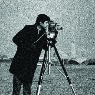
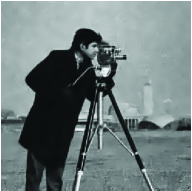
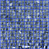
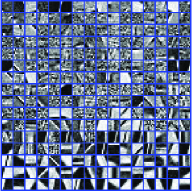
Figure 2: Example of the denoising results for the image “Cameraman” ($\sigma=25$ and $r$=2). (From left to right) The corrupted image, the denoised image by SBDL-VB (28.1587dB), the denoised image by SBDL-Gibbs (28.8380dB), the dictionary trained by SBDL-VB, the dictionary trained by SBDL-Gibbs.

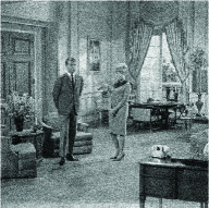
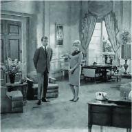
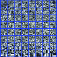
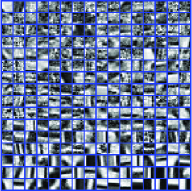
Figure 3: Example of the denoising results for the image “Couple” ($\sigma=25$ and $r$=2). (From left to right) The corrupted image, the denoised image by SBDL-VB (28.4240dB), the denoised image by SBDL-Gibbs (28.8431dB), the dictionary trained by SBDL-VB, the dictionary trained by SBDL-Gibbs.

VI Conclusions

We developed a new Bayesian hierarchical model for learning the overcomplete dictionaries based on a set of training data. This new framework can be considered as an adaptation of the conventional sparse Beysian learning framework to deal with the dictionary learning problem. Specifically, a Gaussian-inverse Gamma hierarchical prior is used to promote the sparsity of the representation. Suitable priors are also placed on the dictionary and the noise variance such that they can be reasonably inferred from the data. We developed a variational Bayesian method and a Gibbs sampler for Bayesian inference. Unlike some of previous methods, the proposed methods do not need to assume knowledge of the noise variance a priori, and can infer the noise variance automatically from the data. The performance of the proposed methods is evaluated using synthetic data. Numerical results show that the proposed methods are able to learn the dictionary with an accuracy considerably better than existing methods, particularly for the case where there is a limited number of training signals. The proposed methods are also applied to image denoising, where superior denoising results are achieved even compared to other state-of-the-art algorithms. Our proposed hierarchical model is also flexible to incorporate additional prior information to enhance the dictionary learning performance.

References

- [1] E. Candés and T. Tao, “Decoding by linear programming,” IEEE Trans. Information Theory, no. 12, pp. 4203–4215, Dec. 2005.
- [2] J. M. Duarte-Carvajalino and G. Sapiro, “Learning to sense sparse signals: simultaneous sensing matrix and sparsifying dictionary optimization,” IEEE Trans. Image Processing, vol. 18, no. 7, pp. 1395–1408, July 2009.
- [3] J. Wright, A. Y. Yang, A. Ganesh, S. S. Sastry, and Y. Ma, “Robust face recognition vis sparse representation,” IEEE Trans. Pattern Analysis and Machine Intelligence, vol. 31, no. 2, pp. 210–227, Feb. 2009.
- [4] M. Aharon, M. Elad, and A. Bruckstein, “K-svd: an algorithm for designing overcomplete dictionaries for sparse representation,” IEEE Trans. Signal Processing, vol. 54, no. 11, pp. 4311–4322, Nov. 2006.
- [5] M. Elad and M. Aharon, “Image denoising via sparse and redundant representations over learned dictionaries,” IEEE Trans. Image Processing, vol. 15, no. 12, pp. 3736–3745, Dec. 2006.
- [6] J. Mairal, F. Bach, and J. Ponce, “Task-driven dictionary learning,” IEEE Trans. Pattern Analysis and Machine Intelligence, vol. 34, no. 4, pp. 791–804, Apr. 2012.
- [7] K. Engan, S. O. Aase, and J. H. Hakon-Husoy, “Method of optimal directions for frame design,” in IEEE International Conference on Acoustics, Speech and Signal Processing, Phoenix, AZ, March 15-19 1999.
- [8] M. Yaghoobi, T. Blumensath, and M. E. Davies, “Dictionary learning for sparse approximations with the majorization method,” IEEE Trans. Signal Processing, vol. 57, no. 6, pp. 2178–2191, June 2009.
- [9] W. Dai, T. Xu, and W. Wang, “Simultaneous codeword optimization (simco) for dictionary update and learning,” IEEE Trans. Signal Processing, vol. 60, no. 12, pp. 6340–6353, Dec. 2012.
- [10] M. Sadeghi, M. Babaie-Zadeh, and C. Jutten, “Learning overcomplete dictionaries based on atom-by-atom updating,” IEEE Trans. Signal Processing, vol. 62, no. 4, pp. 883–891, Feb. 2014.
- [11] M. Zhou, H. Chen, J. Paisley, L. Ren, L. Li, Z. Xing, D. Dunson, G. Sapiro, and L. Carin, “Nonparametric Bayesian dictionary learning for analysis of noisy and incomplete images,” IEEE Trans. Image Processing, vol. 21, no. 1, pp. 130–144, Jan. 2012.
- [12] J. Mairal, F. Bach, J. Ponce, and G. Sapiro, “Online learning for matrix factorization and sparse coding,” Journal of Machine Learning Research, vol. 11, pp. 19–60, 2010.
- [13] K. Skretting and K. Engan, “Recursive least squares dictionary learning algorithm,” IEEE Trans. Signal Processing, vol. 58, no. 4, pp. 2121–2130, Apr. 2010.
- [14] K. Labusch, E. Barth, and T. Martinetz, “Robust and fast learning of sparse codes with stochastic gradient descent,” IEEE Journal of Selected Topics in Signal Processing, vol. 5, no. 5, pp. 1048–1060, 2011.
- [15] D. P. Wipf and B. D. Rao, “An empirical Bayesian strategy for solving the simultaneous sparse approximation problem,” IEEE Trans. Signal Processing, vol. 55, no. 7, pp. 3704–3716, July 2007.
- [16] S. Ji, Y. Xue, and L. Carin, “Bayesian compressive sensing,” IEEE Trans. Signal Processing, vol. 56, no. 6, pp. 2346–2356, June 2008.
- [17] J. Fang, Y. Shen, H. Li, and P. Wang, “Pattern-coupled sparse Bayesian learning for recovery of block-sparse signals,” IEEE Trans. Signal Processing, vol. 63, no. 2, pp. 360–372, Jan. 2015.
- [18] M. Tipping, “Sparse Bayesian learning and the relevance vector machine,” Journal of Machine Learning Research, vol. 1, pp. 211–244, 2001.
- [19] D. G. Tzikas, A. C. Likas, and N. P. Galatsanos, “The variational approximation for Bayesian inference,” IEEE Signal Processing Magazine, pp. 131–146, Nov. 2008.
- [20] A. Gelman, J. B. Carlin, H. S. Stern, D. B. Dunson, A. Vehtari, and D. B. Rubin, Bayesian data analysis. Chapman and Hall/CRC, third edition, 2013.
- [21] C. M. Bishop, Pattern recognition and machine learning. Springer, 2007.