Diagrammatic expansion for positive density-response spectra: Application to the electron gas

Abstract

In a recent paper [Phys. Rev. B 90, 115134 (2014)] we put forward a diagrammatic expansion for the self-energy which guarantees the positivity of the spectral function. In this work we extend the theory to the density response function. We write the generic diagram for the density-response spectrum as the sum of “partitions”. In a partition the original diagram is evaluated using time-ordered Green’s functions on the left-half of the diagram, antitime-ordered Green’s functions on the right-half of the diagram and lesser or greater Green’s function gluing the two halves. As there exist more than one way to cut a diagram in two halves, to every diagram corresponds more than one partition. We recognize that the most convenient diagrammatic objects for constructing a theory of positive spectra are the half-diagrams. Diagrammatic approximations obtained by summing the squares of half-diagrams do indeed correspond to a combination of partitions which, by construction, yield a positive spectrum. We develop the theory using bare Green’s functions and subsequently extend it to dressed Green’s functions. We further prove a connection between the positivity of the spectral function and the analytic properties of the polarizability. The general theory is illustrated with several examples and then applied to solve the long-standing problem of including vertex corrections without altering the positivity of the spectrum. In fact already the first-order vertex diagram, relevant to the study of gradient expansion, Friedel oscillations, etc., leads to spectra which are negative in certain frequency domain. We find that the simplest approximation to cure this deficiency is given by the sum of the zero-th order bubble diagram, the first-order vertex diagram and a partition of the second-order ladder diagram. We evaluate this approximation in the 3D homogeneous electron gas and show the positivity of the spectrum for all frequencies and densities.

I Introduction

Many-body perturbation theory (MBPT) has played an important role in the understanding of the excitation properties of many-electron systems ranging from molecules to solids. An important class of excitations are the neutral excitations in which (in an approximate physical picture) electrons are excited from occupied to unoccupied states. These excitations can, for instance, be induced by external light fields and indeed the optical properties of materials, e.g., the index of refraction, are completely determined by neutral excitations. For the understanding of the excitation spectrum many-body effects are of crucial importance as interactions lead to qualitatively new excited states of the system like plasmons and excitons in solids or the auto-ionizing states in molecules. In many-body theory the neutral excitation spectrum is obtained from the density response function $\chi$ which can be calculated by diagrammatic methods. In practice one does not approximate $\chi$ directly but instead its irreducible part $\mathcal{P}$, called the polarizability. The density response function and the polarizability are related through the integral equation $\chi=\mathcal{P}+\mathcal{P}v\chi$ where $v$ represents the two-body interaction between the electrons. The simplest approximation to $\mathcal{P}$ is the Random Phase Approximation (RPA) introduced by Bohm and Pines Pines and Bohm (1952) to study plasmons in the electron gas. However, many physical phenomena, such as excitons, are not described within the RPA. More complicated approximations involve typically a summation of an infinite class of diagrams, which is usually carried out with the Bethe-Salpeter equation Strinati (1988). For instance, by summing ladder diagrams with a static screened interaction the excitonic properties of many solids are well described Strinati (1988). Nevertheless, there are several other circumstances for which even the static ladder approximation is not enough. In fact, this approximation only allows for single excitations and therefore double and higher excitations are not incorporated Sangalli et al. (2011); Säkkinen et al. (2012). High excitations can significantly contribute to the spectrum of molecular systems. This is, for instance, the case in conjugated polymers, e.g., the polyenes, where the lowest lying singlet states have a double-excitation character Cave et al. (2004). Also for metallic systems there are several physical situations that require a theoretical treatment beyond the RPAHuotari et al. (2008); Sternemann et al. (2005). The calculation of plasmon lifetimes Huotari et al. (2011); Cazzaniga et al. (2011) is one example. Another example is the calculation of the correlation induced double-plasmon excitations Huotari et al. (2008); Sternemann et al. (2005) which has recently been studied both experimentally and theoretically for the simple metals. We also mention that beyond-RPA approximations have been investigated actively in time-dependent density functional theory Ullrich (2012) (TDDFT), a widely used framework to study optical properties of molecules and solids. A key quantity within the TDDFT formalism is the so-called exchange-correlation kernel which depends entirely on corrections beyond the RPA. Several parametrizations of this kernel based on the homogeneous electron gas exist Gross and Kohn (1985); Nifosì et al. (1998); Qian and Vignale (2002) but their application to finite systems is problematic and the development of better approximations is an active research area.

From the viewpoint of diagrammatic MBPT the theoretical description of many-body interactions beyond RPA involves the inclusion of vertex corrections in the Feynman diagrams for the polarizability. Vertex corrections have been studied in several works Glick and Long (1971); Kugler (1975); Sturm and Gusarov (2000); Holas et al. (1979); Devreese et al. (1980); Brosens et al. (1980); Awa et al. (1982a, b); Brosens and Devreese (1984); Engel and Vosko (1990) on the homogeneous electron gas. For this system it was found that first order vertex corrections give rise to negative spectral functions Holas et al. (1979); Brosens and Devreese (1984). Also for finite systems it was found that by either restriction to a certain class of diagrams Sangalli et al. (2011); Hellgren and von Barth (2009) or by truncation to a certain order in the iteration of the Hedin equations Schindlmayr and Godby (1998) the spectral function can become negative. This has two important consequences. First of all, it destroys the physical picture of the photo-absorption spectrum as a probability distribution and secondly it can lead to a density response function with poles off the real axis in the complex frequency plane thereby ruining its analytic and causal properties. Wrong analytic properties were, for instance, found in a study of atomic photo-absorption spectra with vertex corrections included to first order Hellgren and von Barth (2009). Concomitantly it was also shown that the absorption spectrum becomes negative around the energy of the inner-shell transitions. In this work we prove that a density response function with a positive spectrum has the correct analytic properties.

The problem of negative spectra lies in the structure of the vertex correction and therefore the solution must be sought in the way diagrammatic theory is used. In a recent paper Stefanucci et al. (2014) we showed that a similar problem occurs in the spectrum of the Green’s function (which describes the photo-emission spectrum rather than the photo-absorption spectrum). For that case we solved the problem by introducing the concept of “half-diagrams” which we then used to construct a diagrammatic expansion distinct from MBPT. In the present work we show that a similar procedure works for the polarizability too. We apply the theory to derive the lowest order vertex correction which preserves the positivity of the spectrum. We also evaluate this correction for the homogeneous electron gas by using a combination of analytical frequency integrations and numerical Monte-Carlo momentum integrations to evaluate the diagrams.

The paper is divided as follows. In Section II.1 we introduce the spectral function for the density response function and the polarizability and give a diagrammatic proof of their positivity. The basic idea of the proof consists in cutting every diagram into two halves in all possible ways and in recognizing the half-diagrams as the fundamental object of the diagrammatic expansion. Here we also derive the connection between the analytic properties and the positivity of the spectral function. In Section III we put forward a diagrammatic method to generate approximate polarizability with positive spectra. The method is first developed using bare Green’s functions and then extended to dressed Green’s functions. In Section IV we provide some illustrative examples of positive approximations and show how to turn a MBPT approximation into a positive one by adding a minimal set of diagrams. We also address the positivity of approximations generated through the Bethe-Salpeter equation in Section V. In Section VI we evaluate the lowest-order vertex correction which yields a positive spectrum in the homogeneous electron gas. Our conclusions and outlooks are drawn in Section VII.

II Theoretical Framework

II.1 The density response function

We study the properties of the reducible and irreducible response function within the Keldysh Green’s function theory. Although this theory is usually applied in the context of non-equilibrium physics we have found that it also provides a natural and powerful framework for the calculation of equilibrium spectra.

We consider a system of interacting fermions with Hamiltonian

$$\hat{H} = \int d\mathbf{x}\,\hat{\psi}^{\dagger}(\mathbf{x})\hat{h}(\mathbf{x})\hat{\psi}(\mathbf{x})$$ (1)

$$+\frac{1}{2}\int d\mathbf{x}d\mathbf{x}^{\prime}\,\hat{\psi}^{\dagger}(\mathbf{x})\hat{\psi}^{\dagger}(\mathbf{x}^{\prime})v(\mathbf{x},\mathbf{x}^{\prime})\hat{\psi}(\mathbf{x}^{\prime})\hat{\psi}(\mathbf{x}),$$

where the field operators $\hat{\psi}$, $\hat{\psi}^{\dagger}$ annihilate and create a fermion at position-spin $\mathbf{x}=(\mathbf{r}\sigma)$, and $v(\mathbf{x},\mathbf{x}^{\prime})$ is the Coulomb interaction. The one-body part of the Hamiltonian is $\hat{h}(\mathbf{x})=-\frac{\mbox{\boldmath$\nabla$}^{2}}{2m}+qV(\mathbf{x})$, with $V$ the scalar potential and $q$ the fermion charge. Within the Keldysh formalism the correlators are defined on the time-loop contour $\mathcal{C}$ going from $-\infty$ to $+\infty$ (minus-branch $\mathcal{C}_{-}$) and back to $-\infty$ (plus-branch $\mathcal{C}_{+}$). Operators on the minus-branch are ordered chronologically while operators on the plus-branch are ordered anti-chronologically. The Green’s function $G(\mathbf{x}_{1}z_{1},\mathbf{x}_{2}z_{2})$ (like any other two-time correlator) with times $z_{1}$ and $z_{2}$ on the contour embodies four different functions $G^{\alpha\beta}$, $\alpha,\beta=+/-$, depending on the branch $\mathcal{C}_{-},\mathcal{C}_{+}$ to which $z_{1}$ and $z_{2}$ belong. Stefanucci and van Leeuwen (2013); Stefanucci et al. (2014) For both times on the minus branch we have the time-ordered Green’s function $G^{{\scriptscriptstyle-}{\scriptscriptstyle-}}$ whereas for both times on the plus branch we have the anti-time-ordered Green’s function $G^{{\scriptscriptstyle+}{\scriptscriptstyle+}}$. The time-ordered and anti-time-ordered Green’s functions can be expressed in terms of $G^{{\scriptscriptstyle-}{\scriptscriptstyle+}}\equiv G^{<}$ and $G^{{\scriptscriptstyle+}{\scriptscriptstyle-}}\equiv G^{>}$ as follows (omitting the dependence on the position-spin variables)

$$G^{\pm\pm}(t_{1},t_{2})=\theta(t_{1}-t_{2})G^{\gtrless}(t_{1},t_{2})+\theta(t_{2}-t_{1})G^{\lessgtr}(t_{1},t_{2}).$$ (2)

The four functions $G^{\alpha\beta}$ form the building blocks of the following diagrammatic analysis.

The central object of this work is the density response function $\chi$ defined as the contour-ordered product of density deviation operators

$$\chi(\mathbf{x}_{1}z_{1},\mathbf{x}_{2}z_{2})=-i\langle\mathcal{T}_{\mathcal{C}}[\Delta\hat{n}_{H}(\mathbf{x}_{1}z_{1})\Delta\hat{n}_{H}(\mathbf{x}_{2}z_{2})]\rangle,$$

where $\Delta\hat{n}(\mathbf{x})=\hat{n}(\mathbf{x})-\langle\hat{n}(\mathbf{x})\rangle$, the subscript “$H$” implies operators in the Heisenberg picture and $\mathcal{T}_{\mathcal{C}}$ is the contour-ordering operator. The average $\langle\ldots\rangle$ is performed over the many-body state of the system. The greater $\chi^{{\scriptscriptstyle+}{\scriptscriptstyle-}}\equiv\chi^{>}$ and lesser $\chi^{{\scriptscriptstyle-}{\scriptscriptstyle+}}\equiv\chi^{<}$ response functions read

$$\chi^{>}(\mathbf{x}_{1}t_{1},\mathbf{x}_{2}t_{2}) = -i\langle\Delta\hat{n}_{H}(\mathbf{x}_{1}t_{1})\Delta\hat{n}_{H}(\mathbf{x}_{2}t_{2})\rangle$$ (3)

$$\chi^{<}(\mathbf{x}_{1}t_{1},\mathbf{x}_{2}t_{2}) = -i\langle\Delta\hat{n}_{H}(\mathbf{x}_{2}t_{2})\Delta\hat{n}_{H}(\mathbf{x}_{1}t_{1})\rangle$$ (4)

and fulfill the symmetry relation

$$i\chi^{\lessgtr}(\mathbf{x}_{1}t_{1},\mathbf{x}_{2}t_{2})=[i\chi^{\lessgtr}(\mathbf{x}_{2}t_{2},\mathbf{x}_{1}t_{1})]^{*}.$$ (5)

The quantity of interest for the excitation spectrum is the retarded response function

$$\chi^{R}(\mathbf{x}_{1}t_{1},\mathbf{x}_{2}t_{2}) = -i\theta(t_{1}-t_{2})\langle[\hat{n}_{H}(\mathbf{x}_{1}t_{1}),\hat{n}_{H}(\mathbf{x}_{2}t_{2})]\rangle$$

$$= \theta(t_{1}-t_{2})(\chi^{>}-\chi^{<})(\mathbf{x}_{1}t_{1},\mathbf{x}_{2}t_{2}).$$

In equilibrium the Green’s functions $G^{\alpha\beta}$ as well as the response functions $\chi^{\alpha\beta}$ depend on the time-difference $t-t^{\prime}$ and can therefore be conveniently Fourier transformed with respect to this time-difference. In the remainder of the paper we often suppress the dependence on spatial and spin indices and regard all quantities as matrices with one-particle labels. It is easy to verify that the Fourier transform of the retarded response function is given by

$$\chi^{R}(\omega)=\int\frac{d\omega^{\prime}}{2\pi}\frac{\mathcal{B}(\omega^{\prime})}{\omega-\omega^{\prime}+i\eta}$$ (6)

with $\eta$ a positive infinitesimal and spectral function

$$\mathcal{B}(\omega)=i[\chi^{>}(\omega)-\chi^{<}(\omega)].$$ (7)

The matrix function $\mathcal{B}$ contains information on the energy of the neutral excitations and can be measured in optical absorption experiments. From the relation in Eq. (5) we see that $i\chi^{>}(\omega)$ and $i\chi^{<}(\omega)$ are self-adjoint and, therefore, $\mathcal{B}$ is self-adjoint too. The matrix function $i\chi^{>}(\omega)$ vanishes for $\omega<0$ and its average is proportional to the probability of absorbing light with frequency $\omega$ for $\omega>0$. In fact, $i\chi^{>}(\omega)$ is a positive semi-definite (PSD) matrix as it follows directly from the Lehmann representation. Similarly it can be shown that $i\chi^{<}(\omega)$ is PSD and vanishes for $\omega>0$. Thus $\mathcal{B}(\omega)$ is PSD for positive frequencies and negative semi-definite for negative fequencies. Another property which follows directly from the definitions in Eqs. (3) and (4) is the relation $i\chi^{<}(\omega)=[i\chi^{>}(-\omega)]^{\ast}$. For Hamiltonians with time-reversal symmetry, such as in Eq. (1), this relation can also be written as $i\chi^{<}(\omega)=[i\chi^{>}(-\omega)]^{\dagger}$ which implies that $\mathcal{B}(\omega)=-\mathcal{B}(-\omega)$. It is worth noticing for the present work that the PSD property is not guaranteed in diagrammatic approximations to the response function. How to construct PSD diagrammatic approximations is the topic of the next section.

II.2 Positivity of the exact response function

The PSD property of the exact $i\chi^{\lessgtr}(\omega)$ is manifest from the Lehmann representation of this quantity. It is instead less obvious to prove the PSD property from the diagrammatic expansion. Here we provide such a proof and bring to light a diagrammatic structure which forms the basis of a general scheme to construct PSD approximations (or to turn non PSD approximations into PSD ones by adding a minimal set of diagrams). We follow the same line of reasoning as in the recently published work on the PSD property of the self-energy. Stefanucci et al. (2014) The main difference is that the proof for the response function involves intermediate states consisting of particle-hole pairs rather than particle-hole pairs plus a particle or a hole. Since the derivation is otherwise similar we only outline the basic steps and refer to Ref. Stefanucci et al., 2014 for more details. Moreover since the derivation for $\chi^{>}$ is essentially the same as for $\chi^{<}$ we restrict the attention to $\chi^{<}$.

The starting point is Eq. (4) for $\chi^{<}$. Writing explicitly the time-evolution operator $\hat{\mathcal{U}}$ in $\Delta\hat{n}_{H}$ we get

$$i\chi^{<}(1,2)$$

$$=\langle\Psi_{0}|\hat{\mathcal{U}}(t_{0},t_{2})\Delta\hat{n}(\mathbf{x}_{2})\hat{\mathcal{U}}(t_{2},t_{1})\Delta\hat{n}(\mathbf{x}_{1})\hat{\mathcal{U}}(t_{1},t_{0})|\Psi_{0}\rangle,$$

where $|\Psi_{0}\rangle$ is the non-degenerate ground state and the short-hand notation $1=\mathbf{x}_{1}t_{1}$ and $2=\mathbf{x}_{2}t_{2}$ has been introduced. Under the adiabatic assumption the state $|\Psi_{0}\rangle=\hat{\mathcal{U}}(t_{0},\tau)|\Phi_{0}\rangle$ is obtained by propagating the noninteracting ground-state $|\Phi_{0}\rangle$ from the distant future time $\tau$ (eventually we take $\tau\to\infty$) to some finite time $t_{0}$ with an adiabatically switched-on interaction. Therefore

$$i\chi^{<}(1,2) = \langle\Phi_{0}|\hat{\mathcal{U}}(\tau,t_{2})\Delta\hat{n}(\mathbf{x}_{2})\hat{\mathcal{U}}(t_{2},\tau)\sum_{i}|\varphi_{i}\rangle\langle\varphi_{i}|$$ (8)

$$\times\hat{\mathcal{U}}(\tau,t_{1})\Delta\hat{n}(\mathbf{x}_{1})\hat{\mathcal{U}}(t_{1},\tau)|\Phi_{0}\rangle,$$

where we inserted the completeness relation in Fock space $\sum_{i}|\varphi_{i}\rangle\langle\varphi_{i}|=1$. The only states in Fock space which contribute in Eq. (8) have the form

$$|\varphi_{\underline{p}\underline{q}}^{(N)}\rangle\equiv\hat{c}_{q_{N}}^{\dagger}....\hat{c}_{q_{1}}^{\dagger}\hat{c}_{p_{N}}..\hat{c}_{p_{1}}|\Phi_{0}\rangle,$$

where $\hat{c}_{k}$, $\hat{c}_{k}^{\dagger}$ annihilate and create a fermion in the $k$-th eigenstate of the noninteracting problem. In Eq. (8) we can therefore replace

$$\sum_{i}|\varphi_{i}\rangle\langle\varphi_{i}|\rightarrow\sum_{N=1}^{\infty}\frac{1}{N!}\frac{1}{N!}\sum_{\underline{p}\underline{q}}|\varphi_{\underline{p}\underline{q}}^{(N)}\rangle\langle\varphi_{\underline{p}\underline{q}}^{(N)}|,$$ (9)

where $\sum_{\underline{p}\underline{q}}$ denotes integration or summation over the sets $\underline{p}=(p_{1},\ldots,p_{N})$ of occupied states and $\underline{q}=(q_{1},\ldots,q_{N})$ of unoccupied states. The sum starts from $N=1$ since the only state with $N=0$ particle-hole pairs is $|\Phi_{0}\rangle$ and $\langle\Phi_{0}|\Delta\hat{n}|\Phi_{0}\rangle=0$. The prefactor in Eq. (9) originates from the inner product of the intermediate states

$$\langle\varphi_{\underline{p}\underline{q}}^{(N)}|\varphi_{\underline{p}^{\prime}\underline{q}^{\prime}}^{(N^{\prime})}\rangle=\delta_{N,N^{\prime}}\sum_{P,Q\in\pi_{N}}(-)^{P+Q}\delta_{P(\underline{p}),\underline{p}^{\prime}}\delta_{Q(\underline{q}),\underline{q}^{\prime}},$$

where $P$ and $Q$ run over the set $\pi_{N}$ of all possible permutations of $N$ indices and $(-)^{P}$ and $(-)^{Q}$ are the parities of the permutations $P$ and $Q$ respectively. Using Eq. (9) in Eq. (8) we can rewrite the lesser response function as

$$i\chi^{<}(1,2) = \sum_{N=1}^{\infty}\frac{1}{N!}\frac{1}{N!}\sum_{\underline{p}\underline{q}}\mathcal{S}^{(N)}_{\underline{p}\underline{q}}(2)\mathcal{S}^{(N)*}_{\underline{p}\underline{q}}(1),$$ (10)

where the amplitudes $\mathcal{S}$ read

$$\mathcal{S}^{(N)*}_{\underline{p}\underline{q}}(1) =\langle\varphi_{\underline{p}\underline{q}}^{(N)}|\hat{\mathcal{U}}(\tau,t_{1})\Delta\hat{n}(\mathbf{x}_{1})\hat{\mathcal{U}}(t_{1},\tau)|\Phi_{0}\rangle,$$ (11)

$$\mathcal{S}^{(N)}_{\underline{p}\underline{q}}(2) =\langle\Phi_{0}|\hat{\mathcal{U}}(\tau,t_{2})\Delta\hat{n}(\mathbf{x}_{2})\hat{\mathcal{U}}(t_{2},\tau)|\varphi_{\underline{p}\underline{q}}^{(N)}\rangle.$$ (12)

The adiabatic assumption implies that turning the interaction slowly on and off the state $\Phi_{0}$ changes at most by a phase factor: $\hat{\mathcal{U}}(\tau,-\tau)|\Phi_{0}\rangle=e^{i\alpha}|\Phi_{0}\rangle$. Hence we can rewrite the amplitudes as (for more details see Ref. Stefanucci et al., 2014)

$$\mathcal{S}_{\underline{p}\underline{q}}^{(N)*}(\mathbf{x}_{1}t_{1}) = \frac{\langle\Phi_{0}|\mathcal{T}\big{\{}e^{-i\int_{-\tau}^{\tau}d\bar{\tau}\hat{H}(\bar{\tau})}\hat{c}_{p_{1}}^{\dagger}(\tau^{+})\ldots\hat{c}_{p_{N}}^{\dagger}(\tau^{+})\hat{c}_{q_{1}}(\tau)\ldots\hat{c}_{q_{N}}(\tau)\Delta\hat{n}(\mathbf{x}_{1}t_{1})\big{\}}|\Phi_{0}\rangle}{\langle\Phi_{0}|\mathcal{T}\big{\{}e^{-i\int_{-T}^{T}d\bar{\tau}\hat{H}(\bar{\tau})}\big{\}}|\Phi_{0}\rangle}$$ (13a)

$$\mathcal{S}_{\underline{p}\underline{q}}^{(N)}(\mathbf{x}_{2}t_{2}) = \frac{\langle\Phi_{0}|\bar{\mathcal{T}}\big{\{}e^{i\int_{-\tau}^{\tau}d\bar{\tau}\hat{H}(\bar{\tau})}\Delta\hat{n}(\mathbf{x}_{2}t_{2})\hat{c}_{q_{N}}^{\dagger}(\tau)\ldots\hat{c}_{q_{1}}^{\dagger}(\tau)\hat{c}_{p_{N}}(\tau^{+})\ldots\hat{c}_{p_{1}}(\tau^{+})\big{\}}|\Phi_{0}\rangle}{\langle\Phi_{0}|\bar{\mathcal{T}}\big{\{}e^{i\int_{-\tau}^{\tau}d\bar{\tau}\hat{H}(\bar{\tau})}\big{\}}|\Phi_{0}\rangle},$$ (13b)

with $\mathcal{T}$ and $\bar{\mathcal{T}}$ the time-ordering and anti-time-ordering operators respectively. The time argument in the fermion creation and annihilation operators specifies the position of the operators on the time axis, and $\tau^{+}$ denotes a time infinitesimally larger than $\tau$. Equations (13a) and (13b) show that $\mathcal{S}^{(N)*}$ is an interacting time-ordered $(N+1)$-Green’s function whereas $\mathcal{S}^{(N)}$ is an interacting anti-time-ordered $(N+1)$-Green’s function. Hence they can be expanded diagrammatically using Wick’s theorem.van Leeuwen and Stefanucci (2012) The general structure of a $\mathcal{S}$, $\mathcal{S}^{\ast}$ diagram is illustrated in Fig. 1 and resembles half a $\chi$ diagram. The left-half corresponds to $\mathcal{S}^{(N)*}$ with lines given by noninteracting time-ordered Green’s functions $g^{--}$ whereas the right-half corresponds to $\mathcal{S}^{(N)}$ with lines given by noninteracting anti-time-ordered Green’s functions $g^{++}$ (here and in the following we use the letter $g$ to denote the noninteracting Green’s function).

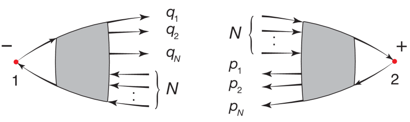
Figure 1: (Color online) Typical diagram for $S^{*}(1)$ (left) and $S(2)$ (right) forming the lesser reducible response function. Labels $p$ and $q$ on the arrows denote quantum numbers of particles and holes respectively, see Eqs. (13).

It is now easy to show that $i\chi^{<}(\omega)$ is PSD. By Fourier transforming $\mathcal{S}$ with respect to $t_{2}$ and $\mathcal{S}^{*}$ with respect to $t_{1}$ we find (omitting the dependence on the spatial and spin variables)

$$i\chi^{<}(t_{1},t_{2}) = \sum_{N=1}^{\infty}\frac{1}{N!N!}\int\frac{d\omega}{2\pi}\frac{d\omega^{\prime}}{2\pi}$$ (14)

$$\times e^{-i\omega t_{2}+i\omega^{\prime}t_{1}}\sum_{\underline{p}\underline{q}}\mathcal{S}_{\underline{p}\underline{q}}^{(N)}(\omega)\mathcal{S}_{\underline{p}\underline{q}}^{(N)*}(\omega^{\prime}).$$

In equilibrium $\chi^{<}$ is invariant under time translations, i.e., it depends on $t_{1}-t_{2}$ only. Imposing time translational invariance on the r.h.s. leads to

$$\sum_{N=1}^{\infty}\frac{1}{N!N!}\sum_{\underline{p}\underline{q}}\mathcal{S}_{\underline{p}\underline{q}}^{(N)}(\omega)\mathcal{S}_{\underline{p}\underline{q}}^{(N)*}(\omega^{\prime})=\mathcal{F}(\omega)\delta(\omega-\omega^{\prime})$$ (15)

with $\mathcal{F}$ some matrix function of the frequency $\omega$. Since for $\omega=\omega^{\prime}$ the l.h.s. is a sum of PSD matrices we conclude that $\mathcal{F}$ is PSD. Inserting Eq. (15) back into Eq. (14) we see that $\mathcal{F}(\omega)$ is the Fourier transform of $i\chi^{<}$ which, therefore, is PSD too.

II.3 Positivity of the exact polarizability

In MBPT it is often more convenient to calculate the irreducible part $\mathcal{P}$ of $\chi$ defined by the equation

$$\chi(z_{1},z_{2}) = \mathcal{P}(z_{1},z_{2})$$ (16)

$$+ \int_{\mathcal{C}}dzdz^{\prime}\,\mathcal{P}(z_{1},z)v(z,z^{\prime})\chi(z^{\prime},z_{2}),$$

where all quantities are matrices in position-spin space and matrix product is implied. The two-body interaction in Keldysh space is given by $v(z,z^{\prime})=v\delta(z,z^{\prime})$. Diagrammatically $\mathcal{P}$ is obtained by removing from $\chi$ all diagrams that can be separated into two pieces by cutting a single interaction line. Like the retarded response function in Eq. (6) the retarded polarizability has the spectral representation

$$\mathcal{P}^{R}(\omega)=\int\frac{d\omega^{\prime}}{2\pi}\frac{\tilde{\mathcal{B}}(\omega^{\prime})}{\omega-\omega^{\prime}+i\eta}$$ (17)

with spectral function

$$\tilde{\mathcal{B}}(\omega)=i[\mathcal{P}^{>}(\omega)-\mathcal{P}^{<}(\omega)].$$ (18)

The matrix functions $\mathcal{P}^{\lessgtr}$ and $\chi^{\lessgtr}(\omega)$ are related by

$$\chi^{\lessgtr}(\omega)=[1-\mathcal{P}^{R}(\omega)v]^{-1}\mathcal{P}^{\lessgtr}(\omega)[1-v\mathcal{P}^{A}(\omega)]^{-1},$$ (19)

where the advanced polarizability $\mathcal{P}^{A}(\omega)=[\mathcal{P}^{R}(\omega)]^{{\dagger}}$. As the exact $\chi^{\lessgtr}$ is PSD this relation implies that $\mathcal{P}^{\lessgtr}$ is PSD too since $[1-\mathcal{P}^{R}v]^{\dagger}=[1-v\mathcal{P}^{A}]$.

Alternatively we can use the diagrammatic expansion of the exact polarizability to show that $\mathcal{P}$ has the PSD property. In fact, the diagrammatic PSD proof for $\chi$ can easily be adapted for $\mathcal{P}$. The removal of (interaction-line) reducible diagrams from $\chi$ is equivalent to the removal of $\mathcal{S}$-diagrams that can be separated into a piece containing the external $\chi$-vertex (either 1 or 2) and a piece containing the $\underline{p}\underline{q}$ vertices by cutting a single interaction line. We refer to these $\mathcal{S}$-diagrams as irreducible $\mathcal{S}$-diagrams or irreducible half-diagrams. It is easy to realize that the product between two irreducible half-diagrams yields an irreducible $\chi$ diagram. If we define $\tilde{\mathcal{S}}$ as the sum of irreducible half-diagrams then the lesser polarizability can be written as

$$i\mathcal{P}^{<}(1,2) = \sum_{N=1}^{\infty}\frac{1}{N!}\frac{1}{N!}\sum_{\underline{p}\underline{q}}\tilde{\mathcal{S}}^{(N)}_{\underline{p}\underline{q}}(2)\tilde{\mathcal{S}}^{(N)*}_{\underline{p}\underline{q}}(1).$$ (20)

Fourier transfroming $\tilde{\mathcal{S}}^{*}$ with respect to $t_{1}$ and $\tilde{\mathcal{S}}$ with respect to $t_{2}$, and carrying out the same analysis as in the case of $\chi$, see Eq. (14), we find that

$$\sum_{N=1}^{\infty}\frac{1}{N!N!}\sum_{\underline{p}\underline{q}}\tilde{\mathcal{S}}_{\underline{p}\underline{q}}^{(N)}(\omega)\tilde{\mathcal{S}}_{\underline{p}\underline{q}}^{(N)*}(\omega^{\prime})=\tilde{\mathcal{F}}(\omega)\delta(\omega-\omega^{\prime}),$$ (21)

where $\tilde{\mathcal{F}}(\omega)$ is a PSD matrix function of the frequency $\omega$. Since $\tilde{\mathcal{F}}$ is the Fourier transform of $i\mathcal{P}^{<}$ then $i\mathcal{P}^{<}$ is PSD too.

II.4 Partitions and cutting rule

For the subsequent development of a PSD diagrammatic theory we need to introduce the concept of partitions of a $\mathcal{P}^{<}$-diagram. This concept naturally arises when we multiply two half diagrams, as we shall show below. Due to the anticommuting nature of the fermionic operators we see from Eq. (13) that a permutation $P$ of the $\underline{p}$ labels and a permutation $Q$ of the $\underline{q}$ labels changes the sign of $\mathcal{S}^{(N)}_{\underline{p}\underline{q}}$ (and hence of $\tilde{\mathcal{S}}^{(N)}$) by a factor $(-)^{P+Q}$. Let then $\{D_{\underline{p}\underline{q}}^{(j)}\}$ with $j\in I_{N}$ be the set of topologically inequivalent diagrams for $\tilde{\mathcal{S}}^{(N)}_{\underline{p}\underline{q}}$ that are not related by a permutation of the $\underline{p}$ and $\underline{q}$ labels. By construction we have the expansion

$$\tilde{\mathcal{S}}^{(N)}_{\underline{p}\underline{q}}=\sum_{j\in I_{N}}\sum_{P,Q\in\pi_{N}}(-)^{P+Q}D^{(j)}_{P(\underline{p})Q(\underline{q})}.$$ (22)

Inserting this expansion in Eq. (20) and using the fact that $\pi_{N}$ is a group we get (for more details see Ref. Stefanucci et al., 2014)

$$i\mathcal{P}^{<}(1,2) = \sum_{N=1}^{\infty}\sum_{j_{1},j_{2}\in I_{N}}\sum_{P,Q\in\pi_{N}}(-)^{P+Q}$$ (23)

$$\times \sum_{\underline{p}\underline{q}}D_{\underline{p}\underline{q}}^{(j_{2})}(2)D^{(j_{1})^{*}}_{P(\underline{p})Q(\underline{q})}(1).$$

Next we observe that the in- and out-going Green’s functions with labels $\underline{p}$ and $\underline{q}$ are evaluated at the largest time $\tau$ and, therefore, they are either a greater or a lesser Green’s function. At zero temperature the noninteracting lesser Green’s function $g^{<}$ satisfies the property

$$\sum_{p}g^{<}_{\mathbf{x}p}(t_{x},\tau)g^{<}_{p\mathbf{y}}(\tau,t_{y})=ig^{<}_{\mathbf{x}\mathbf{y}}(t_{x},t_{y})$$ (24)

with a similar relation for the greater Green’s function. Hence, in the sum $\sum_{\underline{p}\underline{q}}D_{\underline{p}\underline{q}}^{(j_{2})}(2)D^{(j_{1})^{*}}_{P_{1}(\underline{p})Q_{1}(\underline{q})}(1)$ we can replace the product of two $g^{\lessgtr}$ with a single $g^{\lessgtr}$ connecting two internal vertices. The result is a polarizability diagram in which the lines of the left-half are time-ordered Green’s functions, the lines of the right-half are anti-time-ordered Green’s functions and the lines connecting the two halves are either lesser or greater Green’s functions. To represent this type of diagrams we label every internal vertex with a $+$ or a $-$ and introduce the graphical rule according to which a line connecting a vertex with label $\alpha=\pm$ to a vertex with label $\beta=\pm$ is a $g^{\alpha\beta}$. Let us name partition a $\mathcal{P}^{<}$ diagram with decorated $\pm$ vertices. The full $\mathcal{P}^{<}$ diagram is given by the sum of all partitions. The reverse operation of splitting a partition into two half-diagrams consists in cutting all the Green’s function lines between $-$ and $+$ vertices. In the following we refer to this reverse operation as the cutting rule.

Before concluding this section we notice that in Keldsyh formalism a $\mathcal{P}^{<}(t_{1},t_{2})$ diagram is obtained from the corresponding Keldysh diagram $\mathcal{P}(z_{1},z_{2})$ by placing the contour time $z_{1}$ on the minus-branch $\mathcal{C}_{-}$, the contour time $z_{2}$ on the plus-branch $\mathcal{C}_{+}$ and by integrating every internal contour time over $\mathcal{C}$. Thus the $\mathcal{P}^{<}$ diagram is the sum of diagrams with internal vertices decorated in all possible ways. Our derivation shows that decorated diagrams which fall into multiple disjoint pieces by cutting the lines between $-$ and $+$ vertices do not contribute, i.e., they sum up to zero. In fact, these diagrams cannot be written as the product of two half-diagrams.

II.5 Connection between positivity and analytic properties

It follows from the Lehmann representation that the retarded density response function $\chi^{R}(\omega)$ has poles at $\pm\Omega_{j}-i\eta$ where $\Omega_{j}$ are the neutral excitation energies of the system. These poles lie just below the real axis in the complex frequency plane (in the continuous part of the spectrum these are smeared out to a branch cut). Therefore the function $\chi^{R}(z)$ of the complex variable $z$ is an analytic function in the upper half plane $\text{Im}\,z>0$. This analytic property is important in diagrammatic perturbation theory as the density response is an essential ingredient in the calculation of the screened interaction $W$ as is, for instance, used in the $GW$ approximation. A violation of the analytic properties of $\chi^{R}$ would lead to incorrect analytic properties of the Green’s function. It is therefore a relevant question to ask whether any approximate expression for the polarizability $\mathcal{P}^{R}(\omega)$ gives the correct analytic properties of $\chi^{R}(\omega)$. We show here that this is the case whenever $\mathcal{P}^{R}$ is PSD and the interaction matrix $v$ is PSD as well (repulsive interaction).

From the Dyson equation (16) for the response function we can write the retarded component in terms of the polarizability as

$$\chi^{R}(\omega)=\mathcal{P}^{R}(\omega)\left(1-v\mathcal{P}^{R}(\omega)\right)^{-1}.$$ (25)

For our proof it turns out to be advantageous to look at the function $v^{1/2}\chi^{R}v^{1/2}$ which can be written as

$$v^{1/2}\chi^{R}v^{1/2}=\frac{v^{1/2}\mathcal{P}^{R}(\omega)v^{1/2}}{1-v^{1/2}\mathcal{P}^{R}(\omega)v^{1/2}}$$ (26)

where we used the PSD property of $v$ to take the square root operation. The advantage of this expression is that $v^{\frac{1}{2}}\mathcal{P}^{R}(\omega)v^{\frac{1}{2}}$ is PSD whereas $v\mathcal{P}^{R}(\omega)$ does not need to be PSD. Clearly since $v^{1/2}$ is frequency independent it does not change the analytic properties of $\chi^{R}(\omega)$.

We want to know whether $\chi^{R}(z)$ has a pole in upper half of the complex plane, i.e., for $z=x+iy$ with $y>0$. This is either the case when $\mathcal{P}^{R}(z)$ has a pole at $z$ or when $1-v^{1/2}\mathcal{P}^{R}(z)v^{1/2}$ has a zero. From Eq. (17) we have

$$\mathcal{P}^{R}(x+iy)=\int\frac{d\omega^{\prime}}{2\pi}\frac{\tilde{\mathcal{B}}(\omega^{\prime})}{x-\omega^{\prime}+iy}$$ (27)

and therefore

$$\text{Im}\,\mathcal{P}^{R}(z) = -y\int\frac{d\omega^{\prime}}{2\pi}\frac{\tilde{\mathcal{B}}(\omega^{\prime})}{(x-\omega^{\prime})^{2}+y^{2}},$$ (28)

$$\text{Re}\,\mathcal{P}^{R}(z) = \int\frac{d\omega^{\prime}}{2\pi}\frac{(x-\omega^{\prime})\tilde{\mathcal{B}}(\omega^{\prime})}{(x-\omega^{\prime})^{2}+y^{2}},$$ (29)

where we used the short-hand notation $\text{Im}\,\mathcal{P}^{R}=(\mathcal{P}^{R}-\mathcal{P}^{A})/2i$ and $\text{Re}\,\mathcal{P}^{R}=(\mathcal{P}^{R}+\mathcal{P}^{A})/2$. Since $y>0$ and $\tilde{\mathcal{B}}$ is an integrable function both integrals are finite and $\mathcal{P}^{R}(z)$ does not have a pole. It remains to consider the possibility that the operator $1-v^{1/2}\mathcal{P}^{R}(z)v^{1/2}$ has a zero eigenvalue. If this was the case then there would exist an eigenvector $|\lambda\rangle$ for which $\left(1-v^{1/2}\mathcal{P}^{R}(z)v^{1/2}\right)\left|\lambda\right\rangle=0$, and hence

$$\left\langle\lambda\right|1-v^{1/2}\text{Re}\,\mathcal{P}^{R}(z)v^{1/2}\left|\lambda\right\rangle = 0,$$ (30a)

$$\left\langle\lambda\right|v^{1/2}\text{Im}\,\mathcal{P}^{R}(z)v^{1/2}\left|\lambda\right\rangle = 0.$$ (30b)

Using Eq. (28) we rewrite Eq. (30b) as

$$\langle\lambda|v^{1/2}\text{Im}\,\mathcal{P}^{R}(x+iy)v^{1/2}|\lambda\rangle$$

$$=-y\int_{0}^{\infty}\frac{d\omega^{\prime}}{2\pi}\langle\lambda|v^{1/2}\tilde{\mathcal{B}}(\omega^{\prime})v^{1/2}|\lambda\rangle\ell(\omega^{\prime}),$$ (31)

where we took into account that $\tilde{\mathcal{B}}(\omega)=-\tilde{\mathcal{B}}(-\omega)$ to write the integral between $0$ and $\infty$, and defined the function $\ell(\omega)$ according to

$$\ell(\omega)=\left[\frac{1}{(x-\omega)^{2}+y^{2}}-\frac{1}{(x+\omega)^{2}+y^{2}}\right].$$ (32)

The function $\ell(\omega)$ is odd and positive (negative) for positive frequencies and for positive (negative) $x$ values. Therefore $\ell(\omega)$ has a definite sign on the positive frequency axis when $x$ is nonzero. Let us first consider this case, i.e., $x\neq 0$. Since we assumed that $y>0$ and since $\langle\lambda|v^{1/2}\tilde{\mathcal{B}}(\omega^{\prime})v^{1/2}|\lambda\rangle\geq 0$ for positive frequencies the only way to have $\left\langle\lambda\right|v^{1/2}\text{Im}\,\mathcal{P}^{R}(z)v^{1/2}\left|\lambda\right\rangle=0$ is to demand that $\langle\lambda|v^{1/2}\tilde{\mathcal{B}}(\omega^{\prime})v^{1/2}|\lambda\rangle=0$ for all $\omega^{\prime}$. This however, would imply from Eq. (29) that also $\langle\lambda|v^{1/2}\text{Re}\,\mathcal{P}^{R}(z)v^{1/2}|\lambda\rangle=0$ which in turn would imply that $\langle\lambda|1-v^{1/2}\mathcal{P}^{R}(z)v^{1/2}|\lambda\rangle=1$ in contradiction with the assumption. We conclude that $\chi^{R}(z)$ cannot have poles in the upper half plane when $x=\text{Re}\,z\neq 0$. This leaves us with the case $x=0$. For $x=0$ the function $\ell(\omega)=0$ and Eq. (30b) is automatically satisfied. Instead Eq. (30a) reads

$$\langle\lambda|1-v^{1/2}\text{Re}\,\mathcal{P}^{R}(z)v^{1/2}|\lambda\rangle$$

$$=1+2\!\int_{0}^{\infty}\!\!\frac{d\omega^{\prime}}{2\pi}\,\frac{\langle\lambda|v^{1/2}\tilde{\mathcal{B}}(\omega^{\prime})v^{1/2}|\lambda\rangle\omega^{\prime}}{\omega^{\prime 2}+y^{2}}\geq 1$$ (33)

since $v^{1/2}\tilde{\mathcal{B}}v^{1/2}$ is PSD for positive frequencies. In this case too Eq. (30a) cannot be satisfied and therefore $\chi^{R}$ cannot have poles in the upper half plane when $\mathcal{P}^{R}$ and $v$ are PSD.

We mention that the situation is different for negative semidefinite interactions. In this case a similar formula can be defined but with a minus sign in front of the integral. In fact, for a strong enough attraction the right hand side of Eq. (33) can be zero for a well-chosen value of $y$ and consequently $\chi^{R}$ can have poles at $z=iy$ in the upper half plane. The violation of the analytic property occurs for instance in the attractive Hubbard dimer Olsen and Thygesen (2014). As a final remark we note that in a similar fashion one can prove that when the spectral function of the self-energy is PSD then the Green’s function is analytic in the upper half of the complex frequency plane.

Implications to the f-Sum Rule.

The connection between positivity and the analytic structure has important consequences for the f-sum rule, which relates the first momentum of the retarded density response function to the equilibrium density $n_{0}(\mathbf{x})$

$$\int\!\!\omega\chi^{R}(\mathbf{x},\mathbf{x}^{\prime}\omega)\,d\omega=-i\pi\mbox{\boldmath$\nabla$}^{\prime}\cdot\mbox{\boldmath$\nabla$}\left(n_{0}(\mathbf{x}^{\prime})\delta(\mathbf{r}-\mathbf{r}^{\prime})\right)\delta_{\sigma\sigma^{\prime}}.$$ (34)

The derivation of the $f$-sum rule assumes that the integral over the retarded response function can be closed on the upper half-planeStefanucci and van Leeuwen (2013), i.e., $\chi^{R}$ is analytic in this region. In accordance with the results of this Section the analytic assumption is verified for those approximations which fulfill the PSD property.

III PSD diagrammatic expansion

III.1 Formulation with noninteracting Green’s functions

In Section II.1 we have given a diagrammatic proof of the PSD property of the exact polarizability. We further showed that this PSD property is essential to guarantee the correct analytic structure of the density response function. In practice, however, the polarizability is calculated in a MBPT fashion by considering a subclass of Feynman diagrams and hence the PSD property is not, in general, a built-in property of the approximation. The proof given in Section II.3 paves the way for a diagrammatic theory of PSD polarizabilities which is alternative to the more standard MBPT. We have seen that the PSD property follows from the formation of perfect squares and that these squares are the sum of partitions. In contrast MBPT gives a sum of diagrams where each diagram is a sum of partitions but, in general, do not form perfect squares. The most general MBPT approximation to the polarizability when written in terms of partitions (or equivalently in terms of products of half-diagrams) reads

$$i\mathcal{P}^{<}(1,2) = \sum_{N=1}^{\infty}\sum_{(j_{1},j_{2})\in\mathcal{I}_{N}}\sum_{\begin{subarray}{c}P\in\pi^{(j_{1}j_{2})}_{N,p}\\ Q\in\pi^{(j_{1}j_{2})}_{N,q}\end{subarray}}(-)^{P+Q}$$ (35)

$$\times \sum_{\underline{p}\underline{q}}D_{\underline{p}\underline{q}}^{(j_{2})}(2)D^{(j_{1})^{*}}_{P(\underline{p})Q(\underline{q})}(1),$$

where $\mathcal{I}_{N}$ is a subset of the product set $I_{N}\times I_{N}$ and for any given couple $(j_{1},j_{2})$ the sums over $P$ and $Q$ run over a subset $\pi^{(j_{1}j_{2})}_{N,p}$ and $\pi^{(j_{1}j_{2})}_{N,q}$ of the permutation group $\pi_{N}$. The minimal number of additional partitions to add in order to turn the MBPT approximation into a PSD approximation is found by imposing on $\mathcal{P}^{<}$ the mathematical structure in Eq. (23). This is achieved as follows, see also Fig. 2. Let $\{\tilde{I}_{N}^{\alpha}\}$ be a set of disjoint subsets of $I_{N}$ with the property that the union of the product sets

$$\bigcup_{\alpha}\tilde{I}_{N}^{\alpha}\times\tilde{I}_{N}^{\alpha}\supset\mathcal{I}_{N}$$ (36)

and contains the least number of elements of $I_{N}\times I_{N}$. Since the subsets $\tilde{I}_{N}^{\alpha}$ are disjoint the sets $\mathcal{I}_{N}^{\alpha}=\mathcal{I}_{N}\cap(\tilde{I}_{N}^{\alpha}\times\tilde{I}_{N}^{\alpha})$ are disjoint too and due to Eq. (36) we have that $\bigcup_{\alpha}\mathcal{I}_{N}^{\alpha}=\mathcal{I}_{N}$. For any given $\alpha$ we then consider the smallest subgroups of the permutation group $\pi_{N}$ with the property that

$$\tilde{\pi}_{N,p}^{\alpha}\supset\bigcup_{(j_{1}j_{2})\in\mathcal{I}_{N}^{\alpha}}\pi_{N,p}^{(j_{1},j_{2})},$$ (37)

$$\tilde{\pi}_{N,q}^{\alpha}\supset\bigcup_{(j_{1}j_{2})\in\mathcal{I}_{N}^{\alpha}}\pi_{N,q}^{(j_{1},j_{2})}.$$ (38)

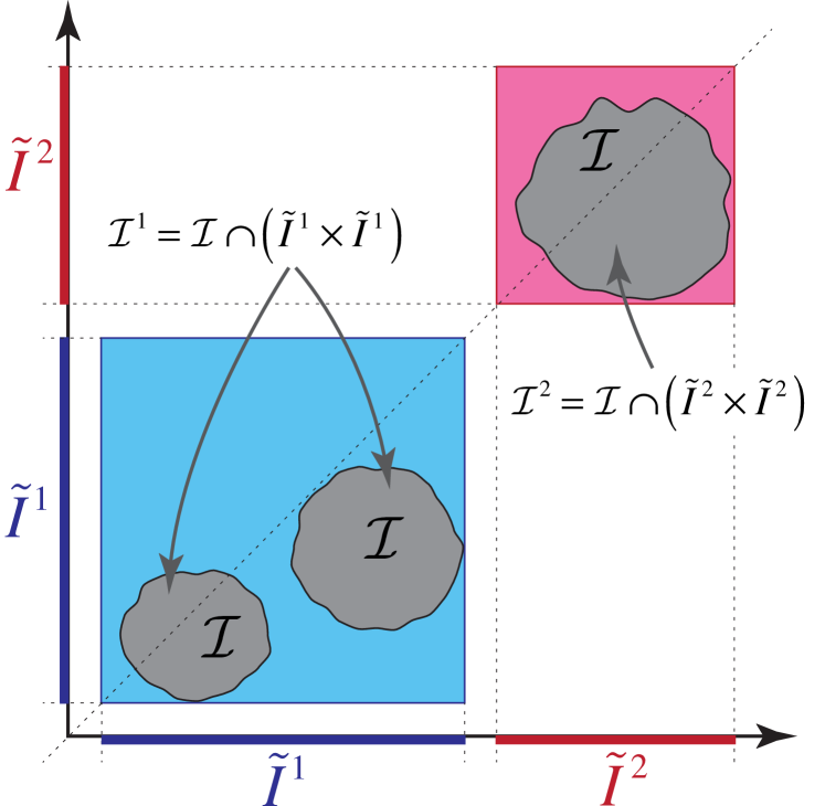
Figure 2: (Color online) Decomposition $\bigcup_{\alpha}\mathcal{I}_{N}^{\alpha}=\mathcal{I}_{N}$ of the $\mathcal{I}_{N}$ subset (denoted as three disjoint gray areas) into a union of (two in this example) product sets.

By construction the polarizability

$$i\mathcal{P}_{\rm PSD}^{<}(1,2) = \sum_{N=1}^{\infty}\sum_{\alpha}\sum_{j_{1},j_{2}\in\tilde{I}_{N}^{\alpha}}\sum_{\begin{subarray}{c}P\in\tilde{\pi}^{\alpha}_{N,p}\\ Q\in\tilde{\pi}^{\alpha}_{N,q}\end{subarray}}(-)^{P+Q}$$ (39)

$$\sum_{\underline{p}\underline{q}}D_{\underline{p}\underline{q}}^{(j_{2})}(2)D^{(j_{1})^{*}}_{P(\underline{p})Q(\underline{q})}(1)$$

contains all partitions of Eq. (35) plus the minimal number of additional partitions to form perfect squares. Consequently the polarizability in Eq. (39) is a diagrammatic PSD approximation. More precisely we can say that a PSD diagrammatic approximation to $\mathcal{P}$ is not the sum of MBPT diagrams, rather it is the sum of partial or decorated diagrams (the partitions) with internal vertices either on the minus or the plus branch of the Keldysh contour. Examples of the PSD procedure are presented in Section IV.

As a final remark we mention that another cutting procedure based on time-ordered half diagrams has been used by Sangalli et al. Sangalli et al. (2011) for the Bethe-Salpeter kernel of the so-called second RPA approximation. In that work the Lehmann product structure was important to satisfy an identity for the determinant of the Bethe-Salpeter kernel which guarantees that no spurious poles occur in the density response function obtained by solving the Bethe-Salpeter equation. However, the procedure proposed in Ref. Sangalli et al., 2011 cannot be used to obtain a direct expression for the spectral function, thus making it difficult to address the PSD property. The difficulty has its origin in the fact that the standard time-ordered formalism is not the natural formalism to express the spectral function. As it has been shown in this work the Keldysh contour technique facilitates enormously the calculation of the spectral function of any diagram, the result being a product of time-ordered and anti-time-ordered half diagrams joined by lesser and greater Green’s function lines.

III.2 Formulation with dressed Green’s functions

In the previous Section we discussed how to generate PSD diagrammatic approximations for the polarizability. A diagrammatic approximation is the sum of partitions and for the PSD property to be satisfied the product of half-diagrams resulting from the cut partitions has to form the sum of perfect squares. The possibility of cutting a partition relies on Eq. (24), according to which the product of two $g^{\lessgtr}$ yields a single $g^{\lessgtr}$. This property, however, is valid only for noninteracting Green’s functions. It would be extremely useful to formulate a cutting rule for partitions written in terms of dressed Green’s functions. The main advantage of a dressed PSD formulation is the absence of polarizability-diagrams with self-energy insertions, thus enabling us to work exclusively with skeleton diagrams.

Here we consider partitions with dressed Green’s function lines and show how to write these partitions as the product of two half-diagrams. We therefore need to replace Eq. (24) with some other equation where $G^{\lessgtr}$ is expressed as the “product” of two functions. The main idea has been discussed in detail in our recent work on the self-energy. Stefanucci et al. (2014) In frequency space the greater and lesser Green’s function read

$$G^{\gtrless}(\mathbf{x}_{1}t_{1},\mathbf{x}_{2}t_{2})=\mp i\int\frac{d\omega}{2\pi}A^{\gtrless}(\mathbf{x}_{1},\mathbf{x}_{2};\omega)e^{-i\omega(t_{1}-t_{2})},$$ (40)

where $A^{<}(\omega)\equiv f(\omega)A(\omega)$ is the removal part of the spectral function $A(\omega)$ whereas $A^{>}(\omega)\equiv(1-f(\omega))A(\omega)$ is the addition part of $A(\omega)$, and $f(\omega)$ is the zero temperature Fermi function. If the self-energy is PSD then both $A^{>}$ and $A^{<}$ are PSD. We expand the matrix $A^{\gtrless}(\omega)$ in terms of its eigenvalues $a_{n}^{\gtrless}(\omega)\geq 0$ and eigenvectors $u_{n}(\omega,\mathbf{x})$

$$A^{\gtrless}(\mathbf{x}_{1},\mathbf{x}_{2};\omega)=\sum_{n}a_{n}^{\gtrless}(\omega)u_{n}(\omega,\mathbf{x}_{1})u_{n}^{*}(\omega,\mathbf{x}_{2})$$ (41)

and define the square root matrix as

$$\sqrt{A^{\gtrless}}(\mathbf{x}_{1},\mathbf{x}_{2};\omega)=\sum_{n}\sqrt{a_{n}^{\gtrless}(\omega)}u_{n}(\omega,\mathbf{x}_{1})u_{n}^{*}(\omega,\mathbf{x}_{2}).$$ (42)

We then make the rule that when cutting a partition the internal lines are $G^{{\scriptscriptstyle-}{\scriptscriptstyle-}}$ for the left half, $G^{{\scriptscriptstyle+}{\scriptscriptstyle+}}$ for the right half, and

$$\sqrt{G^{\gtrless}}(\mathbf{x}_{1}t_{1},\mathbf{x}_{2}t_{2})=\int\frac{d\omega}{2\pi}\sqrt{A^{\gtrless}}(\mathbf{x}_{1},\mathbf{x}_{2};\omega)e^{-i\omega(t_{1}-t_{2})}$$ (43)

for the dangling lines of the two halves. For the reverse operation of gluing the two halves we make the rule that the “product” of two dangling lines is defined according to

$$\int\!d\mathbf{y}dt\,\sqrt{G^{<}}_{\mathbf{x}_{1}\mathbf{y}}(t_{1},t)\sqrt{G^{<}}_{\mathbf{y}\mathbf{x}_{2}}(t,t_{2}) = iG^{<}(1,2),\quad$$ (44a)

$$\int\!d\mathbf{y}dt\,\sqrt{G^{>}}_{\mathbf{x}_{1}\mathbf{y}}(t_{1},t)\sqrt{G^{>}}_{\mathbf{y}\mathbf{x}_{2}}(t,t_{2}) = -iG^{>}(1,2).\quad\quad$$ (44b)

These equations replace Eq. (24) and the analogous for $g^{>}$ in the dressed case. Except that for an additional time-integration Eqs. (44) have the same matrix-product structure as in the undressed case and it is straightforward to verify that the gluing of two half-diagrams gives back the original partition. This implies that if a certain sum of partitions with undressed Green’s functions $g$ is PSD, and hence it can be written as in Eq. (39), then the same sum of partitions with dressed Green’s functions $G$ is PSD too since the corresponding polarizability can be written as

$$i\mathcal{P}_{\rm PSD}^{<}(1,2) = \sum_{N=1}^{\infty}\sum_{\alpha}\sum_{j_{1},j_{2}\in\tilde{I}_{N}^{\alpha}}\sum_{\begin{subarray}{c}P\in\tilde{\pi}^{\alpha}_{N,p}\\ Q\in\tilde{\pi}^{\alpha}_{N,q}\end{subarray}}(-)^{P+Q}$$ (45)

$$\times \int\!d1_{p}\ldots dN_{p}\int\!d1_{q}\ldots dN_{q}$$

$$\times D_{1_{p}\ldots N_{p},1_{q}\ldots N_{q}}^{(j_{2})}(2)\,D^{(j_{1})^{*}}_{P(1_{p}\ldots N_{p})Q(1_{q}\ldots N_{q})}(1),\quad\quad$$

where we introduced the short-hand notation $n_{p}=(p_{n},t^{(p)}_{n})$ ($n=1,\ldots,N$) and $m_{q}=(q_{m},t^{(q)}_{m})$ ($m=1,\ldots,N$) as well as

$$\int dn_{p}=\sum_{p_{n}}\int dt^{(p)}_{n}\;;\quad\int dm_{q}=\sum_{q_{m}}\int dt^{(q)}_{m}.$$ (46)

In Eq. (45) the $D$’s represent the half diagrams with dangling lines $\sqrt{G^{\lessgtr}}$ and external vertices in $1_{p}\ldots N_{p},1_{q}\ldots N_{q}$.

IV Examples

In this section we consider some commonly used diagrammatic approximations to the polarizability and address the PSD property for each of them.

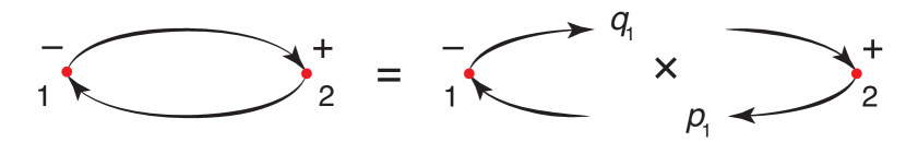
Figure 3: (Color online) Partition and decomposition in half-diagrams of the RPA bubble diagram.

Zeroth order

In Fig. 3 we show the RPA bubble. This diagram can be partitioned in only one way and the decomposition in terms of half-diagrams is shown on the right of the equality sign. According to the cutting rules for dressed diagrams we have

$$D_{1_{p}1_{q}}^{*}(1) = \sqrt{G^{<}}_{\mathbf{x}_{1}p_{1}}(t_{1},t^{(p)}_{1})\sqrt{G^{>}}_{q_{1}\mathbf{x}_{1}}(t^{(q)}_{1},t_{1}),$$

$$D_{1_{p}1_{q}}(2) = \sqrt{G^{<}}_{p_{1}\mathbf{x}_{2}}(t^{(p)}_{1},t_{2})\sqrt{G^{>}}_{\mathbf{x}_{2}q_{1}}(t_{2},t^{(q)}_{1}),$$

and it is straightforward to verify that the RPA bubble can be written as

$$\mathcal{P}^{<}_{\textrm{RPA}}(1,2) = -i\int\,d1_{p}d1_{q}\;D_{1_{p}1_{q}}(2)\,D_{1_{p}1_{q}}^{\ast}(1).$$ (47)

The RPA $\mathcal{P}$ has clearly the structure of Eq. (45) and therefore the spectrum for the response function is positive.

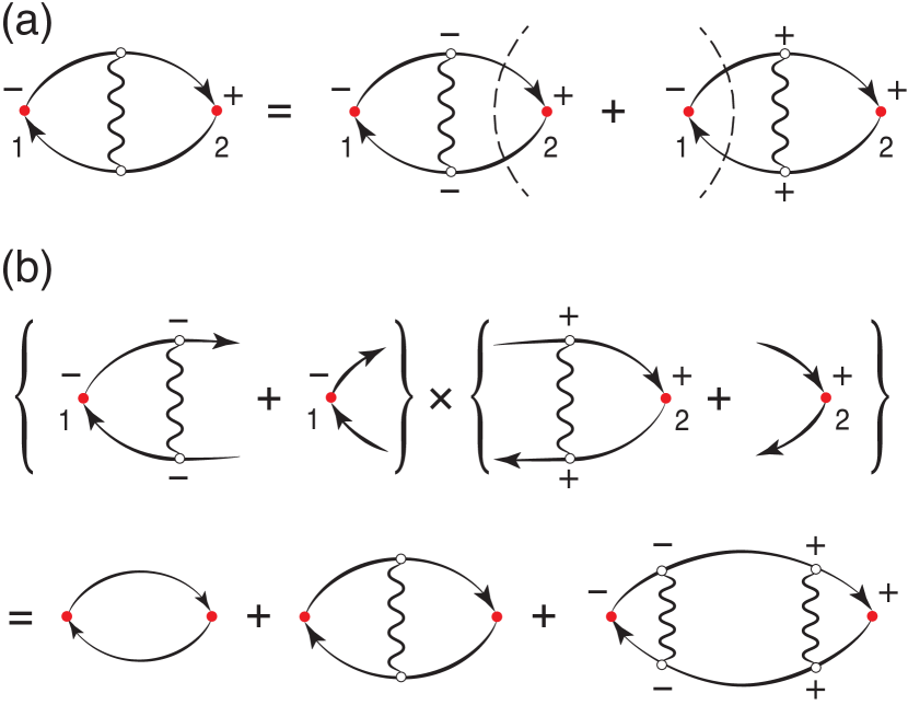
Figure 4: (Color online) (a) Partition and decomposition in half-diagrams of the vertex diagram. The wiggly line denotes the bare interaction $v$. (b) The minimal set of additional partitions to restore the PSD property.

Simplest vertex

In Fig. 4(a) we consider the lowest order (in bare Coulomb interaction) vertex diagram for $\mathcal{P}$. The cutting rules yield only two partitions (on the right of the equality sign) since the bare interaction is local in time and hence $v^{\lessgtr}=0$. From the decomposition in half-diagrams we see that the vertex diagram does not have the structure of Eq. (45). Therefore the PSD property is not guaranteed. The minimal set of partitions to add follows directly from the rules of Section III.1. The result is shown in Fig. 4(b). By multipling the half-diagrams in the curly brackets we get two additional diagrams: the RPA bubble and a partition of the second-order ladder diagram. Here and in the following we use the convention that an internal vertex without $-/+$ labels implies a summation over $-/+$. From this example we also infer that the sum of only the RPA bubble and the vertex diagram is not, in general, PSD. Noteworthy this sum constitute the so called exact exchange (EXX) approximation to the kernel of Time-Dependent Density Functional Theory (TDDFT). The EXX kernel has been calculated in Ref. Hellgren and von Barth, 2009 for the case of closed shell atoms and it was found that it has poles in the upper half of the complex frequency plane. This incorrect analytic behavior is a direct consequence of the relation between the PSD and the analytic properties, as discussed in Section II.5. The correct analytic properties of the EXX kernel can be restored by adding the partition of the second-order ladder diagram shown in Fig. 4(b).

RPA screening

In bulk systems the electron screening plays a crucial role and, therefore, one usually works with interaction-skeletonic diagrams in which the bare interaction $v$ is replaced by some screened interaction $W$. Below we apply the theory developed in Section III.1 to a few diagrammatic approximations in which $W$ is the RPA screened interaction, i.e., $W=v+v\mathcal{P}_{0}W$ where $\mathcal{P}_{0}=-iGG$. Taking into account that partitions with isolated $+/-$ islands do not contribute to the polarizability we immediately conclude that $W^{--}$ and $W^{++}$ should not be cut along the internal Green’s function lines. For the lesser/greater $W$-lines we note that $W^{<}=W^{--}\mathcal{P}_{0}^{<}W^{++}$ and $W^{>}=W^{++}\mathcal{P}_{0}^{>}W^{--}$, see Fig. 5. Therefore the cut of a $W^{\lessgtr}$ amounts to a cut of the two Green’s function lines in $\mathcal{P}_{0}^{\lessgtr}$.

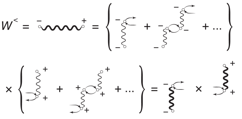
Figure 5: Decomposition of the screened interaction (thick wiggly line) $W^{<}$ in half-diagrams. The decomposition of $W^{>}$ is analogous and given by the bottom diagram with $-\leftrightarrow+$.

Figure 6: (Color online) The simplest PSD approximation to the polarizability in terms of the screened interaction $W$ (thick wiggly line).

The simplest diagrammatic approximation in terms of $W$ is given by the four partitions of Fig. 4(b) in which $v\to W$, see Fig. 6. We observe that the sum of them does not give the full vertex diagram since the partitions with $W^{-+}=W^{<}$ and $W^{+-}=W^{>}$ are missing. These partitions would vanish if, instead of the RPA $W$, we used an externally given static $W$ like, e.g., a Yukawa-type interaction. We will come back to this example in Section VI where we give explicit expressions of the diagrams of Fig. 6 for the electron gas and show the crucial role played by the second-order ladder diagram for the PSD property.

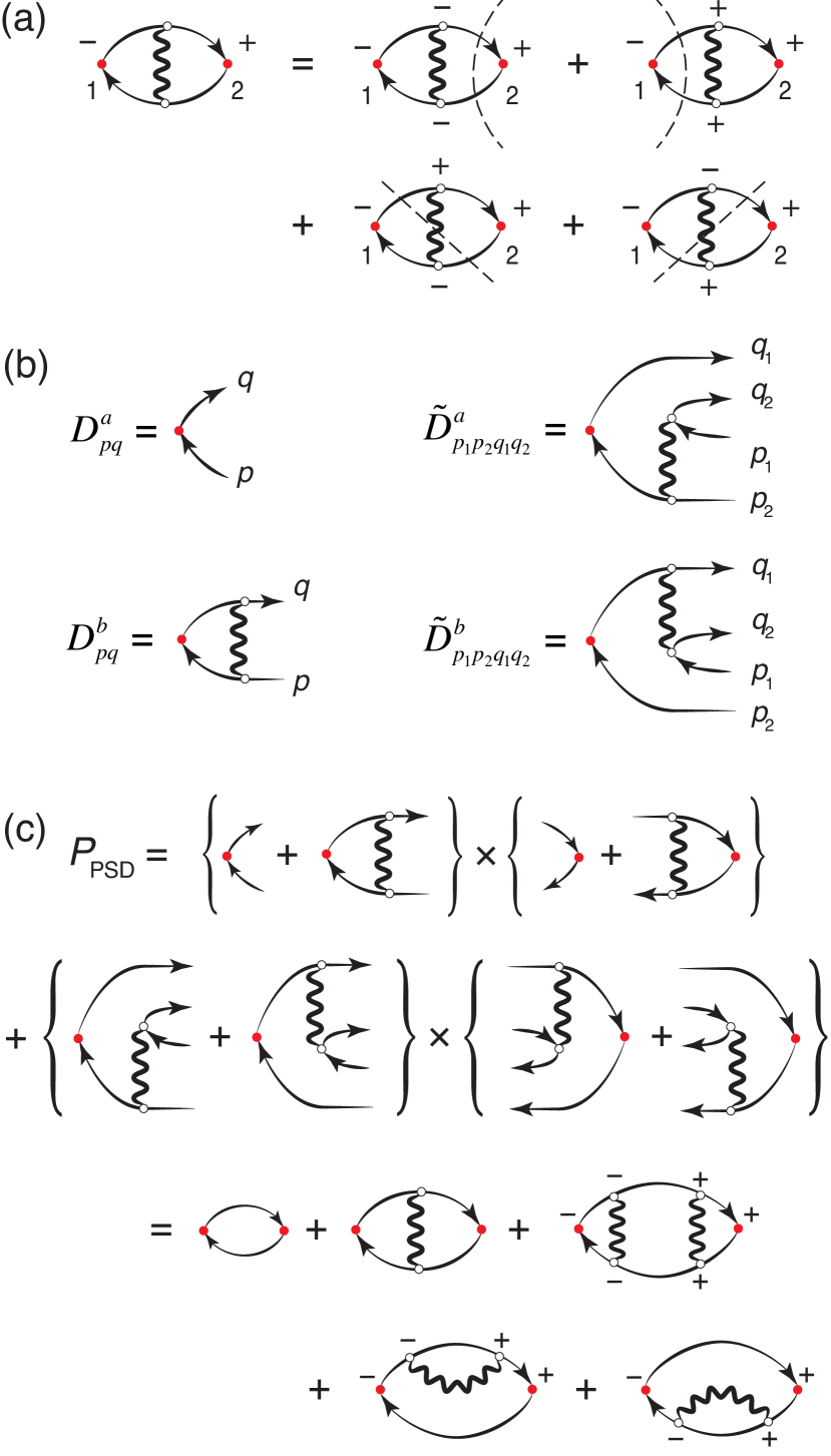
Figure 7: (Color online) (a) Decomposition of the vertex diagram with screened interaction line into half-diagrams. (b) Constituent half-diagrams. (c) The resulting PSD polarizability.

First order

The decomposition into half-diagrams of the full first order (in screened Coulomb interaction) vertex diagram is shown in Fig. 7(a). Since the times of the internal vertices can be different (nonlocal interaction) we have four different partitions. In two of them we only cut the $G$-lines while in the other two we also cut the $W$-line (the cut of the $W$-line leads to half-diagrams with four dangling lines). Thus, we have two half-diagrams with one particle-hole ($D^{(a)}$ and $D^{(b)}$) and two half-diagrams with two particle holes ($\tilde{D}^{(a)}$ and $\tilde{D}^{(b)}$). Naming each half-diagram as shown in the figure 7(b) we can write (omitting the integrals over the vertices to be glued as well as dependence on the external vertices)

$$i\mathcal{P}^{<}=D^{(a)}D^{(b)^{\ast}}+D^{(b)}D^{(a)^{\ast}}+\tilde{D}^{(a)}\tilde{D}^{(b)^{\ast}}+\tilde{D}^{(b)}\tilde{D}^{(a)^{\ast}},$$ (48)

which does not have the structure of Eq. (45) and hence it is not PSD. Applying the rules of Section III.1 we find the minimal set of partitions to add in order to restore the PSD property

$$i\mathcal{P}^{<}_{\rm PSD}=\sum_{ij=a,b}D^{(i)}D^{(j)^{\ast}}+\sum_{ij=a,b}\tilde{D}^{(i)}\tilde{D}^{(j)^{\ast}},$$ (49)

where in each of the sums the indices $i$ and $j$ independently take values $a$, $b$. The resulting diagrammatic approximation to $\mathcal{P}$ is illustrated in Fig. 7(c). The important message of this example is that the additional diagrams are not necessarily skeletonic in $G$ (occurrence of self-energy insertions, viz. the last two diagrams in the figure). Thus attention has to be paid when restoring the PSD property using a dressed $G$. In order to avoid double countings one should not dress the $G$ with the same self-energy appearing in the diagrams of the PSD polarizability.

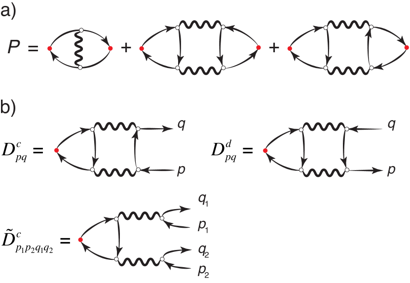
Figure 8: (Color online) (a) Diagrammatic approximation to the polarizability. (b) Constituent half-diagrams in addition to those presented in Fig. 7(b).

GW exchange-correlation kernel

We conclude this section with another important example. In Ref. von Barth et al., 2005 it was shown how to generate conserving approximations to the TDDFT kernel using a variational principle à la Luttinger-Ward. Luttinger and Ward (1960) The underlying variational functional of Luttinger-Ward is a functional of the bare interaction $v$ and the Green’s function $G$. To lowest order in $v$ one can show that the variational principle leads to the EXX approximation. It is possible to extend the Luttinger-Ward idea to functionals of the screend interaction $W$ and the Green’s function $G$.Almbladh et al. (1999) In this case the lowest order approximation is the “time-dependent $GW$” (TD$GW$) approximation; and the TDDFT kernel (more precisely its convolution with two $\mathcal{P}_{0}$’s) is given by the sum of the diagrams in Fig. 8(a) (see also Sec. III.B of Ref. von Barth et al., 2005). These are the same diagrams evaluated by Sternemann et al. Sternemann et al. (2005) and by Huotari et al. Huotari et al. (2008) for the electron gas in order to explain the double-plasmon shoulder in the absorption spectrum of sodium. By partitioning each diagram of the approximate polarizability we find that $\mathcal{P}^{<}$ can be written in terms of four half-diagrams with one particle-hole and three half-diagrams with two particle-holes. Some of them have already been introduced in Fig. 7(b), the new ones are shown in Fig. 8(b) and the expression of $\mathcal{P}^{<}$ in terms of them is (again omitting integrals and the dependence on the external vertices)

$$i\mathcal{P}^{<} = \tilde{D}^{(a)}\left(\tilde{D}^{(a)}_{PQ}+\tilde{D}^{(b)}+\tilde{D}^{(b)}_{PQ}+\tilde{D}^{(c)}_{P}+\tilde{D}^{(c)}_{Q}\right)^{\ast}$$ (50)

$$+ \tilde{D}^{(b)}\left(\tilde{D}^{(b)}_{PQ}+\tilde{D}^{(a)}+\tilde{D}^{(a)}_{PQ}+\tilde{D}^{(c)}_{P}+\tilde{D}^{(c)}_{Q}\right)^{\ast}$$

$$+ \tilde{D}^{(c)}\left(\tilde{D}^{(c)}+\tilde{D}^{(c)}_{PQ}+\tilde{D}^{(a)}_{P}+\tilde{D}^{(a)}_{Q}+\tilde{D}^{(b)}_{P}+\tilde{D}^{(b)}_{Q}\right)^{\ast}$$

$$+ D^{(a)}\left(D^{(b)}+D^{(c)}+D^{(d)}\right)^{\ast}$$

$$+ \left(D^{(b)}+D^{(c)}+D^{(d)}\right)D^{(a)^{\ast}},$$

where the half-diagrams with subindex $P$ (and/or $Q$) are calculated at permuted values $2_{p},1_{p}$ (and/or $2_{q},1_{q}$). For instance, $\tilde{D}^{(c)}\tilde{D}^{(c)^{\ast}}_{PQ}$ is a short form of the integral

$$\int\!d1_{p}d2_{p}\int\!d1_{q}d2_{q}\;\tilde{D}^{(c)}_{1_{p}2_{p}1_{q}2_{q}}(2)\,\tilde{D}^{(c)^{\ast}}_{2_{p}1_{p}2_{q}1_{q}}(1).$$

The polarizability of Eq. (50) is not, in general, PSD since it does not have the form of Eq. (45). The minimal addition to restore the PSD property follows from the rules of Section III.1 which give

$$i\mathcal{P}^{<}_{\rm PSD}=\sum_{ij=a,b,c,d}D^{(i)}D^{(j)^{\ast}}+\sum_{ij=a,b,c}\sum_{P,Q\in\pi_{2}}\tilde{D}^{(i)}\tilde{D}^{(j)^{\ast}}_{PQ}.$$ (51)

The first sum leads to $4\times 4=16$ partitions whereas the second sum leads to $3\times(2^{2}\times 3)=36$ partitions. In Fig. 9 some representative ones are shown.

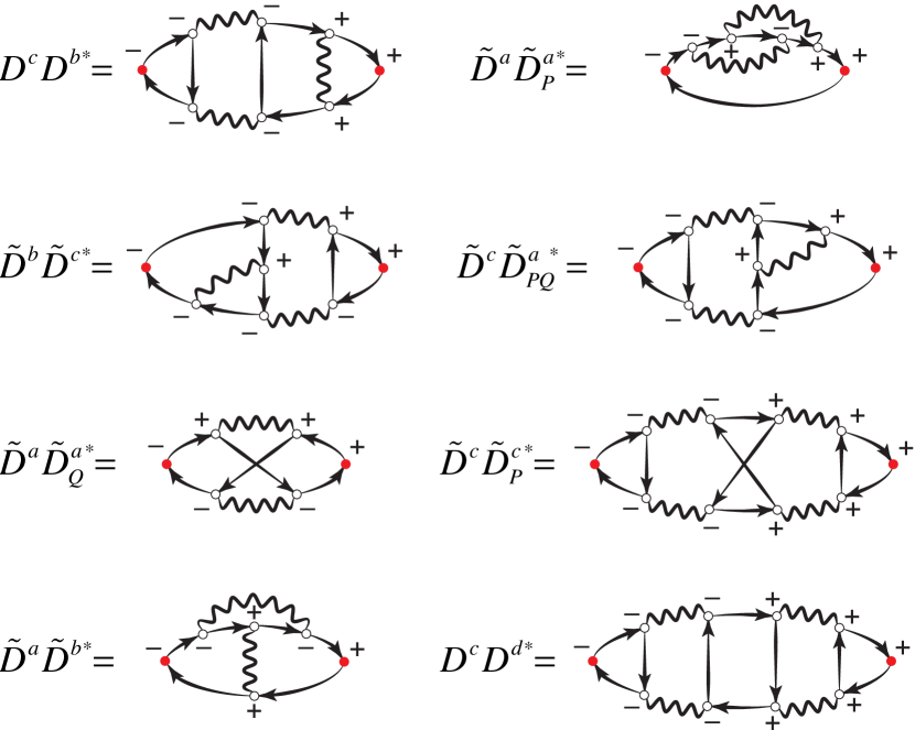
Figure 9: (Color online) A few additional partitions of Eq. (51).

V On the Positivity of the Bethe-Salpeter kernel

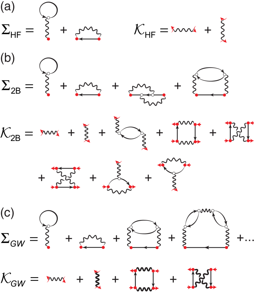
Figure 10: (Color online) Self-energy and the corresponding BSE kernel for (a) Hartree-Fock (b) Second order Born and (c) $GW$ approximations.

So far we have studied only approximations to the irreducible response function consisting of a finite number of diagrams. However, typically approximations beyond the RPA involve an infinite series of diagrams conveniently resummed through the Bethe-Salpeter equation (BSE) Salpeter and Bethe (1951); Strinati (1988). A natural question to ask is whether the corresponding spectral function is PSD. To answer we have to find the diagrammatic structure encoded in the kernel of the BSE. The BSE is a Dyson-like equation for the four-point reducible polarizability $\mathcal{L}(12;34)$ and it is obtained as the response to a non-local scalar potential $u(4,3)$ Strinati (1988)

$$\mathcal{L}(12;34) = \!-\frac{\delta G(1,2)}{\delta u(4,3)}=\mathcal{L}_{0}(12;34)$$

$$+ \!\!\!\!\!\!\!\!\int\!d(5678)G(1,5)G(7,3)\mathcal{K}(56;78)\mathcal{L}(82;64)\quad$$ (52)

where $\mathcal{L}_{0}(12;34)=G(1,4)G(2,3)$ and the four-point reducible kernel $\mathcal{K}$ is given by $\mathcal{K}(12;34)=-i\delta\Sigma(1,3)/\delta G(4,2)$. The variation of the Green’s function is related to the two-particle Green’s function and therefore $\mathcal{L}$ is related to the two-particle excitation spectrum. By taking the limit $3\to 1^{+}$ and $4\to 2^{+}$ we obtain an equation for the response function since $\chi(1,2)=i\mathcal{L}(12;1^{+}2^{+})$.

From standard approximations to the self-energy, e.g., Hartree-Fock (HF), second order Born (2B) or the $GW$ approximation, we can derive a diagrammatic expression for the kernel $\mathcal{K}$, see Fig. 10. By defining a two-particle irreducible and one interaction line irreducible kernel $\tilde{\mathcal{K}}$ as (see also Fig. 11(a))

$$\tilde{\mathcal{K}}(12;34)=\mathcal{K}(12;34)-i\delta(1,3)\delta(2,4)v(1,2),$$ (53)

we can write the polarizability as an infinite series of response diagrams

$$\mathcal{P}(1,2)=\mathcal{P}_{0}(1,2)+i\!\int\!d(3456)\,G(5,1)G(1,3)\tilde{\mathcal{K}}(34;56)$$

$$\times G(4,2)G(2,6)+\ldots.\quad$$ (54)

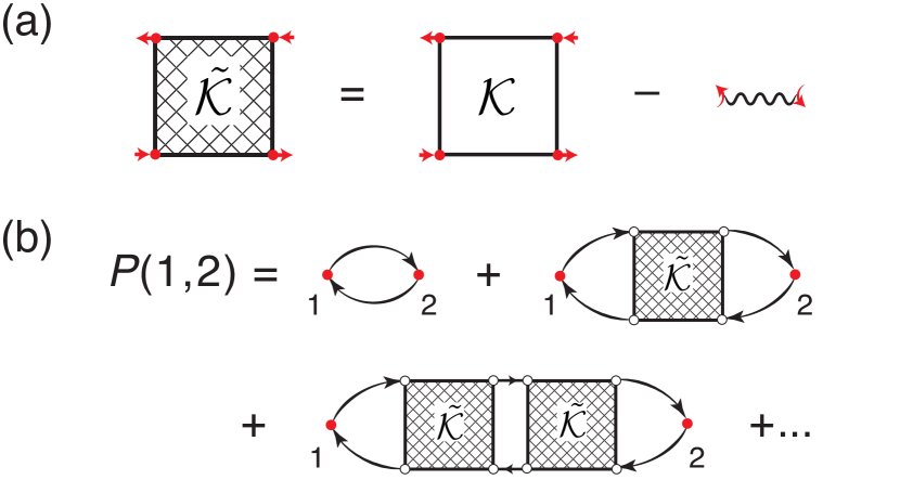
Figure 11: (Color online) (a) Two-particle irreducible and one interaction line irreducible kernel $\tilde{\mathcal{K}}$. (b) The diagrammatic expression for the polarizability in terms of BSE kernel $\tilde{\mathcal{K}}$.

where $\mathcal{P}_{0}(1,2)=-iG(1,2)G(2,1)$. The diagrammatic expression for this equation is shown in Fig. 11(b). By using the kernels in Fig. 10 we obtain the approximations shown in Fig. 12. The HF approximation for the BSE kernel yields the diagrams shown in the Fig. 13, which we can easily see to be PSD. From this example we also deduce that if a kernel cannot be partitioned then the corresponding polarizability is PSD. A commonly used approximation to study the exitonic properties of solids is the static $GW$ approximation Strinati (1988); Sangalli et al. (2011); Olsen and Thygesen (2014) with kernel

$$\tilde{\mathcal{K}}^{(0)}_{\textrm{GW}}(12;34)=i\delta(1,2)\delta(3,4)W(1,3),$$ (55)

where the functional derivative of $W$ with respect to $G$ is neglected.

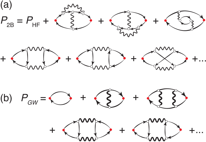
Figure 12: (Color online) Approximations for the polarizability by using BSE kernel with various self-energy approximations. (a) 2B polarizability. (b) $GW$ polarizability.

This approximation leads to the polarizability of Fig. 13 in which the bare interaction lines are replaced by statically screened ones. Therefore, the static $GW$ approximation yields PSD spectra. For the full $GW$ approximation some of the half-diagrams have been already worked out in Fig. 8 and the resulting diagrams after the gluing procedure have been shown in Fig. 9. From this figure we see that the PSD procedure leads to new types of diagrams which are not obtained via the iteration of the BSE. Thus, we conclude that the BSE polarizability with $GW$ kernel does not necessarily have PSD spectra. The same is true for the 2B approximation as can be seen from the half-diagrams generated by the last diagram on the first line of Fig. 12. By applying the PSD procedure we will generate diagrams which are not obtained via iteration of the BSE. Therefore, even the 2B approximation is not a PSD approximation for the BSE. These simple examples show that the kernels generated by conserving $\Phi$-derivable self-energies Baym and Kadanoff (1961); Baym (1962); Luttinger and Ward (1960) do not need to be PSD.

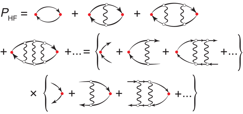
Figure 13: (Color online) The polarizability calculated from the HF BSE kernel is PSD.

VI Numerical results

As an illustration of our method we compute the spectral functions $\tilde{\mathcal{B}}(k,\omega)$ of the polarizability $\mathcal{P}(k,\omega)$ for the three-dimensional homogeneous electron gas. For convenience we introduce here the spectral functions for the positive $\tilde{\mathcal{B}}^{>}(k,\omega)$ and negative $\tilde{\mathcal{B}}^{<}(k,\omega)$ frequencies and scale them by the factor of $8\pi\alpha r_{s}$ in order to make the zeroth order (the Lindhard polarization function) density independent

$$\tilde{\mathcal{B}}^{(0)}(k,\omega)=\left\{\begin{array}[]{lr}\frac{\omega}{k}&\frac{|\omega|}{k}\leq 2-k,\\ \frac{1}{k}-\frac{1}{4k}\big{(}k-\frac{\omega}{k}\big{)}^{2}&\;\;|2-k|<\frac{|\omega|}{k}\leq 2+k,\end{array}\right.$$ (56)

where we expressed $k$ in units of the Fermi momentum $k_{F}=1/(\alpha r_{s})$ and $\omega$ in units of the Fermi energy $\epsilon_{F}=k_{F}^{2}/2$. Here $\alpha=[4/(9\pi)]^{1/3}$ and $r_{s}$ is the standard measure of the system’s density–the Wigner-Seitz radius–expressed in units of the Bohr radius.

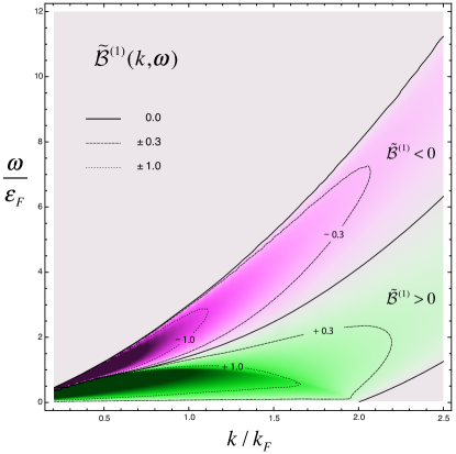
Figure 14: (Color online) Distribution of positive (green) and negative (pink) values of the first order spectral function of the vertex diagram in Fig. 4(b) in the $k-\omega$ plane. The lines represent isospectral curves with values $\pm 0.3$ (dashed) $\pm 0.1$ (dotted) and $0$ (solid).

In 1958 J. Hubbard diagrammatically studied the correlation energy of a free-electron gas Hubbard (1958) and introduced what is now known as the local field factor ($f(k,\omega)$, same notation as in the original manuscript is used). A very interesting introduction to the historical development of this concept and its importance for the density functional theory can be found in Ref. Giuliani and Vignale, 2005. In essence, it provides a simple way to go beyond RPA both in the treatment of the density response function and the total energy of a many-body system and relates between the exact and zeroth order polarizabilities $v(k)f(k,\omega)=[\mathcal{P}(k,\omega)]^{-1}-[\mathcal{P}^{(0)}(k,\omega)]^{-1}$. Thus, every advancement in the calculation of the proper density response function leads to our improved knowledge of the local field factor and, correspondingly, of the density functionals. After Hubbard’s original static approximation $f(k,\omega)\approx k^{2}/(k^{2}+k_{F}^{2})$ there were numerous works to compute the local field factor using the above relation, notably the exact long and short wavelength limits (see Ref. Giuliani and Vignale, 2005 and references therein). Diagrammatically, the simplest case of the first order diagrams (in terms of the bare Coulomb interaction) was computed in a concise form by Engel and Vosko Engel and Vosko (1990) for the static case. Importantly, they considered two types of diagrams, the proper first order response and the first order self-energy insertions and demonstrated a rather large cancellations between these two contributions. In a full generality the frequency dependent first-order results were obtained by Holas, Aravind, and Singwi Holas et al. (1979). However, the analytic form is rather complicated and can only be expressed in terms of a one-dimensional integral. We will use these results for a comparison and, therefore, numerical details concerning the evaluation of this integral are presented in Appendix A. In fact, already the first order vertex diagram of Fig. 4(b) demonstrates the problem of standard MBPT. In Fig. 14 we depict its momentum and energy resolved spectral function $\tilde{\mathcal{B}}^{(1)}$ computed according to the expression of Ref. Holas et al., 1979. The pink shaded area denotes a part of the particle-hole continuum where the 1st order spectral function is negative.

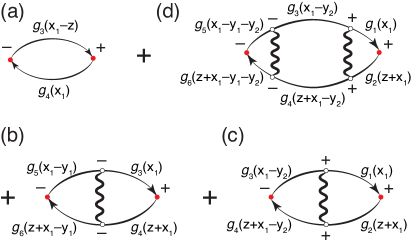
Figure 15: (Color online) Sum of these zero to second order polarizability diagrams yields positive spectral function. Lines with arrows denote the electron propagator $G_{0}(k,\omega)$, whereas wavy-lines stand for bare or screened Coulomb interaction. Vertices are labeled with $+$ ($-$) if they belong to the positive (negative) time ordering part of the Keldysh contour.

In order to solve this problem we use our method and consider the irreducible polarizability diagrams shown in Fig. 4(b) and Fig. 6: a particular second order diagram must be added in order to compensate for the negative sign of $\tilde{\mathcal{B}}^{(1)}$. The two sets of diagrams are topologically identical, however, the first one is given in terms of bare Coulomb, while the second contains screened interacting lines. To be general we will start with the second more complicated case and derive the first case by making the limit $w(k)\rightarrow\Omega(k)\rightarrow\infty$ in the plasmon pole approximation for the screened Coulomb interaction:

$$W_{0}^{--}(k,\omega)=\frac{v(k)}{2}\!\left[\frac{w(k)}{\omega-\Omega(k)+i\eta}-\frac{w(k)}{\omega+\Omega(k)-i\eta}\right].$$ (57)

In this expression $w(k)=t(k)\Omega^{2}(0)/\Omega(k)$, $0\leq t(k)\leq 1$ is the plasmonic spectral weight, and $\Omega(k)$ is the plasmonic dispersion with $\Omega(0)=4\sqrt{\alpha r_{s}/(3\pi)}\epsilon_{F}$, where $\epsilon_{F}$ is the Fermi energy. For the numerical integration we define the bare time-ordered Green’s function asStefanucci et al. (2014)

$$G_{0}^{--}(k,\omega)=\frac{B(k)}{\omega-\epsilon_{k}-i\eta}+\frac{A(k)}{\omega-\epsilon_{k}+i\eta}.$$ (58)

In non-interacting systems $B(k)=n_{k}$ and $A(k)=1-n_{k}$ with $n_{k}$ denoting the occupation of the state with momentum $k$. The frequency integrations can be done completely analytically (facilitated by the mathematica computer algebra system (CAS)) whereas for the remaining momentum integrations one has to rely on numerics Pavlyukh et al. (2013). The starting point are the four diagrams depicted at Fig. 15. The momentum flows are explicitly shown. There are in general many possibilities to assign momenta to propagators. Our choice is dictated by the matter of convenience and is not unique. In order to further simplify notations we adopt the following short forms: $A_{i}\equiv A(x_{i})$, $B_{i}\equiv B(x_{i})$, $C_{i}\equiv\frac{1}{2}v(y_{i})w(y_{i})$, and introduce the function

$$\mathcal{H}_{i}(a,\Omega)=\frac{A_{i}}{a-\Omega-\epsilon_{i}}+\frac{B_{i}}{a+\Omega-\epsilon_{i}}.$$

We also recall that $\tilde{\mathcal{B}}^{>}(k,|\omega|)=\tilde{\mathcal{B}}^{<}(k,-|\omega|)$. Therefore, it is sufficient to consider only one case, e.g., $\omega>0$. The results of frequency integration are

$$\tilde{\mathcal{B}}_{a}^{<}(z,\zeta)\!\! = \!\!-\pi\!\!\int\!\!\frac{d^{3}x_{1}}{(2\pi)^{3}}A_{3}B_{4}\delta(\zeta-\epsilon_{4}+\epsilon_{3}),$$ (59a)

$$\tilde{\mathcal{B}}_{b}^{<}(z,\zeta)\!\! = \!\!-\pi\!\!\int\!\!\frac{d^{3}x_{1}}{(2\pi)^{3}}\!\int\!\!\frac{d^{3}y_{1}}{(2\pi)^{3}}\frac{\mathcal{H}_{6}(\epsilon_{4},\Omega_{1})-\mathcal{H}_{5}(\epsilon_{3},\Omega_{1})}{\epsilon_{3}-\epsilon_{4}-\epsilon_{5}+\epsilon_{6}}C_{1}A_{3}B_{4}\delta(\zeta-\epsilon_{4}+\epsilon_{3}),$$ (59b)

$$\tilde{\mathcal{B}}_{c}^{<}(z,\zeta)\!\! = \!\!-\pi\!\!\int\!\!\frac{d^{3}x_{1}}{(2\pi)^{3}}\!\int\!\!\frac{d^{3}y_{2}}{(2\pi)^{3}}\frac{\mathcal{H}_{2}(\epsilon_{4},\Omega_{2})-\mathcal{H}_{1}(\epsilon_{3},\Omega_{2})}{\epsilon_{3}-\epsilon_{4}-\epsilon_{1}+\epsilon_{2}}C_{2}A_{3}B_{4}\delta(\zeta-\epsilon_{4}+\epsilon_{3}),$$ (59c)

$$\tilde{\mathcal{B}}_{d}^{<}(z,\zeta)\!\! = \!\!-\pi\!\!\int\!\!\frac{d^{3}x_{1}}{(2\pi)^{3}}\!\int\!\!\frac{d^{3}y_{1}}{(2\pi)^{3}}\!\int\!\!\frac{d^{3}y_{2}}{(2\pi)^{3}}\frac{\mathcal{H}_{6}(\epsilon_{4},\Omega_{1})-\mathcal{H}_{5}(\epsilon_{3},\Omega_{1})}{\epsilon_{3}-\epsilon_{4}-\epsilon_{5}+\epsilon_{6}}\frac{\mathcal{H}_{2}(\epsilon_{4},\Omega_{2})-\mathcal{H}_{1}(\epsilon_{3},\Omega_{2})}{\epsilon_{3}-\epsilon_{4}-\epsilon_{1}+\epsilon_{2}}C_{1}C_{2}A_{3}B_{4}\delta(\zeta-\epsilon_{4}+\epsilon_{3}).\;\;$$ (59d)

They are quite general and can be used to obtain e.g. plasmonic contribution. If, however, results for bare Coulomb interacting lines are needed we take the limits and obtain:

$$\tilde{\mathcal{B}}_{a}^{<}(z,\zeta)\!\! = \!\!-\pi\!\!\int\!\!\frac{d^{3}x_{1}}{(2\pi)^{3}}A_{3}B_{4}\delta(\zeta-\epsilon_{4}+\epsilon_{3}),$$ (60a)

$$\tilde{\mathcal{B}}_{b}^{<}(z,\zeta)\!\! = \!\!-\pi\!\!\int\!\!\frac{d^{3}x_{1}}{(2\pi)^{3}}\int\!\!\frac{d^{3}y_{1}}{(2\pi)^{3}}v(y_{1})\frac{A_{6}-A_{5}}{\epsilon_{3}-\epsilon_{4}-\epsilon_{5}+\epsilon_{6}}A_{3}B_{4}\delta(\zeta-\epsilon_{4}+\epsilon_{3}),$$ (60b)

$$\tilde{\mathcal{B}}_{c}^{<}(z,\zeta)\!\! = \!\!-\pi\!\!\int\!\!\frac{d^{3}x_{1}}{(2\pi)^{3}}\int\!\!\frac{d^{3}y_{2}}{(2\pi)^{3}}v(y_{2})\frac{A_{2}-A_{1}}{\epsilon_{3}-\epsilon_{4}-\epsilon_{1}+\epsilon_{2}}A_{3}B_{4}\delta(\zeta-\epsilon_{4}+\epsilon_{3}),$$ (60c)

$$\tilde{\mathcal{B}}_{d}^{<}(z,\zeta)\!\! = \!\!-\pi\!\!\int\!\!\frac{d^{3}x_{1}}{(2\pi)^{3}}\int\!\!\frac{d^{3}y_{1}}{(2\pi)^{3}}\int\!\!\frac{d^{3}y_{2}}{(2\pi)^{3}}v(y_{1})v(y_{2})\frac{A_{6}-A_{5}}{\epsilon_{3}-\epsilon_{4}-\epsilon_{5}+\epsilon_{6}}\frac{A_{2}-A_{1}}{\epsilon_{3}-\epsilon_{4}-\epsilon_{1}+\epsilon_{2}}A_{3}B_{4}\delta(\zeta-\epsilon_{4}+\epsilon_{3}).$$ (60d)

Notice that the spectral functions in Eqs. (59) and (60) are denoted by the same symbol because their type can always be inferred from the context. In these equations $A$, $B$, and $\epsilon$ quantities are labeled by the momenta as shown at Fig. 15. For instance

$$B_{5}\equiv\left\{\begin{array}[]{cc}1&|x_{1}-y_{1}-y_{2}|\leq k_{F},\\ 0&|x_{1}-y_{1}-y_{2}|>k_{F},\end{array}\right.$$

and $\epsilon_{5}=(x_{1}-y_{1}-y_{2})^{2}/2$. $\tilde{\mathcal{B}}_{a}(z,\zeta)\equiv\tilde{\mathcal{B}}^{(0)}(z,\zeta)$ is obviously the Lindhard polarization function. $\tilde{\mathcal{B}}_{b}(z,\zeta)$ and $\tilde{\mathcal{B}}_{c}(z,\zeta)$ differ only by the permutation of indices and, therefore, are equal in view of the left-right symmetry of the corresponding diagrams. There are no other topologically identical diagrams of the first order, i.e. $\tilde{\mathcal{B}}_{b}(z,\zeta)+\tilde{\mathcal{B}}_{c}(z,\zeta)=\tilde{\mathcal{B}}^{(1)}(z,\zeta)$. There are two more partitions of the second order having the same topology as $\tilde{\mathcal{B}}_{d}(z,\zeta)$. They have different combinations of pluses and minuses assigned to the vertices and are not considered here, hence $\tilde{\mathcal{B}}_{d}(z,\zeta)=\tilde{\mathcal{B}}^{(2)}(z,\zeta)$.

Before analyzing numerical results let us first notice a different proportionality of each perturbative order to the electron density. Because we scaled all spectral functions such that $\tilde{\mathcal{B}}^{(0)}$ is density independent it is easy to see that $\tilde{\mathcal{B}}^{(n)}=\mathcal{O}((\alpha r_{s})^{n})$. Thus, the sum of four terms in Eqs. (60) is given by a quadratic polynomial in terms of $\alpha r_{s}$. The requirement of its positivity leads, therefore, to the following inequality

$$\mathcal{D}=(\tilde{\mathcal{B}}_{b}^{<}(z,\zeta))^{2}-\tilde{\mathcal{B}}_{a}^{<}(z,\zeta)\tilde{\mathcal{B}}_{d}^{<}(z,\zeta)\leq 0,$$ (61)

which should hold for all values of frequency and momenta for at least one density. This ensures the positivity of the spectral function at all densities. Mathematically, inequality (61) is the Cauchy-Schwarz inequality applied to the integrals of half-diagrams.

The 1st and 2nd order expressions (Eqs. (60)) as well as the analytic result of Holas et al. [Holas et al., 1979] (Appendix A) suffer from the logarithmic singularities of the integrated functions. This poses additional challenges for numerics. We tackle this problem by introducing a small imaginary part $i\delta$ into the energy denominators. The Monte-Carlo integration is performed as in Ref. Stefanucci et al., 2014 with the use of Mersenne twister 19937 random number generator Haramoto et al. (2008). Additional complication arises due to the use of bare rather than the plasmonically screened Coulomb interaction, i.e. even large momentum transfers are possible. In this case we can still map the integration variables to the $[0,1]$ interval by the logarithmic scaling. For instance, we represent the vector $\mathbf{y}_{1}$ as follows $r_{1}=-p\log(x_{1})$, $\cos(\theta_{1})=-1+2x_{2}$, $\phi_{1}=2\pi x_{3}$, where $p$ is some suitably chosen constant  and $x_{i}\in[0,1]$. Thus, $d^{3}y_{1}=\frac{4\pi p}{x_{1}}dx_{1}dx_{2}dx_{3}$.

Let us look now at the results of the Monte-Carlo integration for a density of $r_{s}=3$. The full momentum ($0.1k_{F}\leq k\leq 2.5k_{F}$) and energy ($0\leq\omega\leq 12\epsilon_{F}$) resolved spectral functions are shown in Fig. 16. On this graph the numerically produced points are projected on the analytically known results depicted as surfaces. For the second order analytical expressions are not known, therefore, only points are shown. At small momenta the spectral functions diverge, therefore we introduced some truncation. The sum of all tree terms, $\tilde{\mathcal{B}}_{\rm PSD}$, is always positive as an example of a cross-section at $k=1.2k_{F}$ in Fig. 17 demonstrates. For some frequencies, however, $\tilde{\mathcal{B}}_{\rm PSD}(k,\omega)$ is rather small and lies within the error bar of the Monte Carlo simulation.

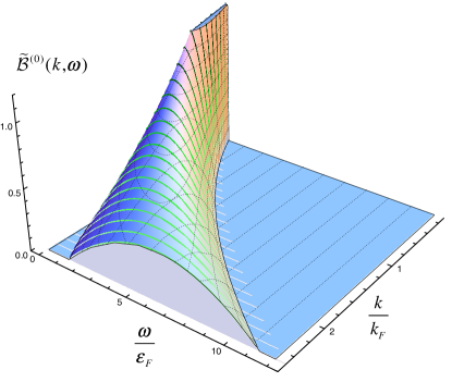
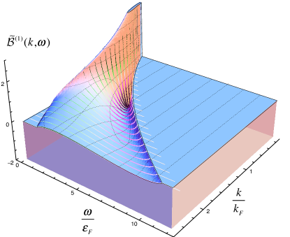
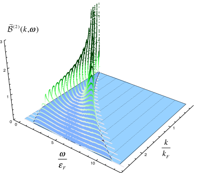
Figure 16: (Color online) The scaled spectral function for the polarizability $\mathcal{P}$ of homogeneous electron gas at $r_{s}=3$. Surfaces denote exact analytical results: 0th order is given by the Lindhard function (Eq. (56)) and 1st order is computed according to 1d integral representation of Holas et al.Holas et al. (1979). Dots denote numerical results obtained by the Monte-Carlo calculation.

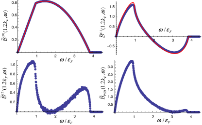
Figure 17: (Color online) Cross-sections of the results in Fig. 16 for the momentum value of $k=1.2k_{F}$ and density $r_{s}=3$. Top left: zeroth order contribution $\tilde{\mathcal{B}}^{(0)}$. Top right: first order contribution $\tilde{\mathcal{B}}^{(1)}$. Bottom left: second order contribution $\tilde{\mathcal{B}}^{(2)}$. Bottom right: the sum of all three contributions $\tilde{\mathcal{B}}_{\rm PSD}$ which is positive. Dots (blue) denote numerical Monte Carlo results. Solid lines (red) stand for analytical results.

The domain where $\tilde{\mathcal{B}}^{(1)}(k,\omega)$ is negative is not bounded, see again Fig. 14. Thus, corrections originating from $\tilde{\mathcal{B}}^{(2)}(k,\omega)$ qualitatively modify the behavior of the spectral function at any momentum. This, in view of the Hilbert transform in Eq. (17), leads to a modification of the real part of the response function. The general conclusion is that the cutting procedure for PSD spectra works as it should. The addition of the second order vertex diagram correctly removes the negative parts of the response function to first order in the vertex.

Cancellation between vertex corrections and self-energy insertions

Although our example is the simplest one that illustrates the PSD diagrammatic theory, it is too simple from a physical point of view. The main reason is that we used bare propagators $G_{0}$ and bare interactions $v$. The first order vertex diagram is not the only first order diagram as we missed two first order diagrams that contain exchange self-energy insertions. If we had used an expansion in dressed Green’s functions $G$ and dressed interactions $W$ such diagrams would not appear as in that case we could restrict ourselves to skeleton diagrams. However, in an expansion in $G_{0}$ and $v$ they become relevant. In particular the self-energy diagrams lead to a cancellation of the divergent small $k$-behavior of the spectral function $\tilde{\mathcal{B}}^{(1)}(k,\omega)$. For the case $\omega=0$ this as been explicitly demonstrated by Engel and Vosko Engel and Vosko (1990). It would therefore be a natural step to include the first order self-energy diagrams as it would, for instance, guarantee the existence of a gradient expansion for the exchange-correlation energy, see below. Taken together these diagrams can be expanded in a power series in terms of the momenta which plays an important role in determining the gradient expansion of the exchange-correlation energy functional in density functional theory. It is well known that in the lowest order the gradient correction to the exchange-correlation functional can be expressed as Engel and Vosko (1990); van Leeuwen (2013)

$$\Delta E_{xc}[n_{0},\delta n(\mathbf{q})]=\frac{1}{2}\int\frac{d^{3}q}{(2\pi)^{3}}\delta n(\mathbf{q})\frac{\Delta\mathcal{P}(\mathbf{q},0)}{[\mathcal{P}(\mathbf{q},0)]^{2}}\delta n(-\mathbf{q}),$$

where $\delta n$ is the density variation with respect to the density $n_{0}$ of the homogeneous system, and $\Delta\mathcal{P}(\mathbf{q},0)$ denotes corrections to the response function from the first and higher order diagrams. Therefore, the inclusion of $\tilde{\mathcal{B}}^{(2)}$ will certainly modify the gradient expansion coefficients, e.g, due to Engel and Vosko Engel and Vosko (1990). However, to have a well-defined gradient expansion one has to add the self-energy diagrams as well. Unfortunately, a simple addition would destroy the positivity of the resulting spectral function again. This was noticed e.g. by Brosens and Devreese Brosens and Devreese (1984) and is illustrated in Fig.18, where we also display the contribution of the self-energy diagram ($\tilde{\mathcal{B}}^{(1,\mathrm{Se})}(k,\omega)$) calculated using the analytic expression of Holas et al.Holas et al. (1979).

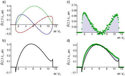
Figure 18: (Color online) Spectral functions at momentum $k=2.5k_{F}$ and density $r_{s}=3$. (a) In addition to previously considered zeroth order ($\tilde{\mathcal{B}}^{(0)}$, dotted) and first order ($\tilde{\mathcal{B}}^{(1)}$, short dash) a contribution of the diagrams with self-energy insertion ($\tilde{\mathcal{B}}^{(1,\mathrm{Se})}$, long dash) is shown. (b) Sum of three terms in panel (a). (c) Second order contribution, $\tilde{\mathcal{B}}^{(2)}$. (d) $\tilde{\mathcal{B}}_{\rm PSD}$ including the first order self-energy diagrams (dots), solid line as in (b), shaded area denotes second order contribution. In order to cancel small negative spectral function at the edge of particle-hole continuum ($\omega=1.25\epsilon_{F}$) inclusion of more diagrams as shown at Fig. 19 is required.

Therefore, if we desire to include the self-energy diagrams and still wish to guarantee positivity we have to apply our PSD theory and consider an extended set of diagrams. The minimal set that achieves this goal is displayed in Fig. 19 which apart from additional self-energy diagrams also contains mixed self-energy and vertex diagrams. Rather than developing codes to evaluate these additional diagrams we found it more worthwhile to explore approximations that involve dressed Green’s functions and interactions. First of all, the dressing of the interaction reduces the singular behavior of the diagrams and secondly they reduce the number of diagrams to be evaluated since we can then stick to skeletonic diagrams. However, since this requires an extensive discussion by itself we will address this topic in a future publication. An alternative route was undertaken by Brosens, Devreese and Lemmens in a series of works Brosens et al. (1976, 1977); Devreese et al. (1980); Brosens et al. (1980) using the variational solution of the linearized equation of motion for the electron density distribution function. They have shown that the first term in a series expansion of the variational result for the local field factor yields the lowest order diagrammatic result. Since such solution also contains higher order terms the spectral function is positive. However, it is not free from singularities suggesting again possible benefits of working with dressed Green’s functions and interactions.

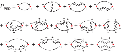
Figure 19: (Color online) $\mathcal{P}_{\rm PSD}$ obtained from the cutting procedure including the first order self-energy diagrams.

VII Conclusions and outlook

Vertex corrections in diagrammatic approximations to the polarizability are known to be crucial for capturing double and higher particle-hole excitations, excitons, multiple plasmon excitations, etc. as well as for estimating excitation life-times. However, the straighforward inclusion of MBPT vertex diagrams can lead to negative spectra, a drawback which discouraged the scientific community to develop numerical recipes and tools for the evaluation of these diagrams in molecules and solids. In this work we provided a simple set of rules to select special combinations of diagrams yielding a positive spectrum.

In our formulation every MBPT diagram is written as the sum of partitions, and every partition is cut into half-diagrams. We recognized that they are the half-diagrams the fundamental quantities for a PSD expansion. In fact, the sum of squares of half-diagrams corresponds to a special selection of partitions which is PSD by construction. The requirement of positivity on the spectrum is important not only for the physical interpretation of the results but also for the correct analytic structure of the polarizability. We demonstrated that a PSD polarizability cannot generate a (retarded) density response function with poles in the upper-half of the complex frequency plane. This is a critical property to converge self-consistent numerical schemes. Although the PSD diagrammatic expansion put foward in this work applies equally well to bare as well as dressed Green’s functions a word of caution is due in the dressed case. The gluing of skeletonic, i.e., self-energy insertion-free, half-diagrams can lead to nonskeletonic polarizability diagrams. In order to avoid the double counting of some of the diagrams it is therefore necessary to use Green’s functions dressed with self-energy diagrams distinct from those appearing in $\mathcal{P}$.

A natural way to sum to infinite-order a subclass of polarizability diagrams is through the BSE, an integral equation with kernel given by the functional derivative of the self-energy with respect to the Green’s function. Due to the popularity of the BSE we also addressed the issue whether the polarizability which solves the BSE is PSD for conserving self-energies, and found a negative answer. The counter example is provided by the self-energy in the second-Born or $GW$ approximations. Noteworthy these self-energies yield a positive spectrum for the Green’s function Stefanucci et al. (2014); therefore neither a conserving nor a PSD self-energy does necessarily generate a PSD polarizability through the BSE.

The simplest approximation with vertex corrections is the first-order ladder diagram. This diagram has been calculated both in finite and bulk systems and it is known to be not PSD. How to include vertex corrections without altering the positivity of the spectrum has been a long-standing problem, which we have solved in this work. By adding a partition of the second-order ladder diagram we obtained the simplest PSD approximation with vertex corrections. We then evaluated this approximation in the 3D homogeneous electron gas and confirmed numerically the correctness of our PSD theory. We stress again that the PSD property alone does not necessarily guarantee physically meaningful spectra. In fact, the PSD spectrum with vertex corrections has un unphysical divergency at zero frequency and momentum. The inclusion of bubble diagrams with first-order exchange self-energy insertions removes this divergency but destroys the PSD property. We worked out the minimal set of diagrams to turn this extended approximation into a PSD one. The evaluation of the resulting extra diagrams is within reach of our code but it requires a considerable numerical effort and it goes beyond the scope of the present work.

VIII Acknowledgments

AMU would like to thank the Alfred Kordelin Foundation for support. GS acknowledges funding by MIUR FIRB Grant No. RBFR12SW0J. YP acknowledges support by the DFG through SFB762. RvL would like to thank the Academy of Finland for support.

Appendix A Numerical evaluations of the analytical expressions for the first order polarizability

As in the rest of the text we measure the momentum and the energy in units of the Fermi momentum $k_{F}=1/(\alpha r_{s})$ and the Fermi energy $\epsilon_{F}=k_{F}^{2}/2$. In older papers $k_{F}^{2}$ as the energy unit was used Holas et al. (1979). This must be taken into account when comparing. Also notice that Engel and Vosko measured momentum in terms of $2k_{F}$. It is natural because the first order polarizability has a logarithmic singularity at this point. The imaginary part of the dielectric function resulting from the first order polarizability is given by

$$\text{Im}\,\varepsilon(q,\omega)=\frac{8}{\pi}\frac{\alpha^{2}r_{s}^{2}}{k^{4}}\left(F^{\mathrm{Ex}}\Big{(}k,\frac{\omega}{2}\Big{)}+F^{\mathrm{Se}}\Big{(}k,\frac{\omega}{2}\Big{)}\right),$$ (62)

whereas the scaled spectral functions considered in Sec. VI read

$$\tilde{\mathcal{B}}^{(1)}(k,\omega) = \frac{4}{\pi}\frac{\alpha r_{s}}{k^{2}}F^{\mathrm{Ex}}\Big{(}k,\frac{\omega}{2}\Big{)},$$ (63)

$$\tilde{\mathcal{B}}^{(1,\mathrm{Se})}(k,\omega) = \frac{4}{\pi}\frac{\alpha r_{s}}{k^{2}}F^{\mathrm{Se}}\Big{(}k,\frac{\omega}{2}\Big{)},$$ (64)

with the function $F$ non-zero at two domains in $k-\omega$ plane (restricted by the Heaviside $\theta$-functions):

$$F^{\mathrm{Ex,Se}}(k,\bar{\omega})=\theta\Big{[}1-\Big{(}\frac{\bar{\omega}}{k}-\frac{k}{2}\Big{)}^{2}\Big{]}\Phi^{\mathrm{Ex,Se}}\Big{(}\frac{\bar{\omega}}{k}-\frac{k}{2},k\Big{)}\\ -\theta\Big{[}1-\Big{(}\frac{\bar{\omega}}{k}+\frac{k}{2}\Big{)}^{2}\Big{]}\Phi^{\mathrm{Ex,Se}}\Big{(}-\frac{\bar{\omega}}{k}-\frac{k}{2},k\Big{)},$$ (65)

and in turn

$$\Phi^{\mathrm{Se}}(\nu,k) = kf_{L}\big{(}\big{[}(k+\nu)^{2}+\left(1-\nu^{2}\right)\big{]}^{1/2}\big{)}$$ (66)

$$\quad\quad\quad-(k+\nu)f_{L}(k+\nu)+\nu f_{L}(\nu),\quad$$

$$\Phi^{\mathrm{Ex}}(\nu,k) = -G_{1}(\nu)+G_{2}(\nu+k,1-\nu^{2}),$$ (67)

where $f_{L}$ is the Lindhard function

$$f_{L}(z)=\frac{1}{2}+\frac{1-z^{2}}{4z}\log\left|\frac{z+1}{1-z}\right|,$$

and $G_{1}$ is (cf. Eq. (2.15) of Holas et al.in Ref. [Holas et al., 1979])

$$G_{1}(\nu) = \frac{1}{4}(1-\nu^{2})g\Big{(}\frac{1-\nu}{1+\nu}\Big{)}-\frac{1}{2}\nu$$

$$\times \big{(}(1-\nu)\log(1-\nu)+(1+\nu)\log(1+\nu)-2\log 2\big{)},$$

with $g(z)=\mathrm{Li}_{2}(-z)-\mathrm{Li}_{2}\big{(}-1/z\big{)}$ represented in terms of the polylogarithm functions. The second function is more involved, it is given by the Hilbert transform which has to be computed numerically:

$$G_{2}(x,y)=-\frac{1}{4}\int_{-1}^{1}d\xi\frac{T(\xi,x,y)}{\xi-x}.$$ (69)

If $|x|<1$ the simplest way to avoid singularity is to exclude a small ($|x_{a}-x_{b}|<\epsilon$) interval $x\in(x_{a},x_{b})\subset(-1,1)$ from the integration. Finally, the $T(\xi,x,y)$ function is defined as (cf. Eqs. (2.18-2.23) of Holas et al. in Ref. [Holas et al., 1979]):

$$T(\xi,x,y) = \left(\frac{a_{1}}{2t}-\frac{a_{1}}{2}+\left(1-\xi^{2}\right)(1-t)\right)$$ (70)

$$\times \log\left(2t\left(1-\xi^{2}\right)+a_{1}\right)-y\log\left(a_{1}\right)$$

$$+ \left(1-\xi^{2}\right)(t-\log(t)-1)$$

in terms of auxiliary functions ($\gamma=x^{2}+y$, $a_{1}=2(\xi-x)^{2}$, $a_{2}=4(1-\xi^{2})(\xi-x)^{2}$, $a_{3}=2\xi(\xi-x)-1$, $\lambda=\frac{a_{2}}{(\gamma+a_{3})^{2}}$) and

$$t(\xi,x,y)=\left\{\begin{array}[]{lc}\frac{(\xi-x)^{2}}{a_{3}+\gamma}&|\lambda|\leq\epsilon,\\ \frac{a_{3}+\gamma}{\left(1-\xi^{2}\right)}\frac{\sqrt{1+\lambda}-1}{2}&|\lambda|>\epsilon.\end{array}\right.$$ (73)

From the imaginary part of the polarization function the real part can be computed through the Hilbert transform. For the static case $\omega=0$ we have:

$$\mathrm{Re}\chi^{(1)}(k,0)\!\! = \!\!\frac{2}{\pi^{3}k^{2}}\!\int_{\epsilon}^{k(k+2)}\frac{d\omega}{\omega}\left[F^{\mathrm{Ex}}\big{(}k,\frac{\omega}{2}\big{)}+F^{\mathrm{Se}}\big{(}k,\frac{\omega}{2}\big{)}\right]$$ (74)

$$= \!\!-\frac{1}{\pi^{3}}\left[a\left(\frac{k}{2}\right)+b\left(\frac{k}{2}\right)\right],$$

where for $a(q)$ and $b(q)$ there are analytic expressions due to Engel and VoskoEngel and Vosko (1990):

$$b(q) = \frac{1-q^{2}}{8q^{2}}\log^{2}\left|\frac{1+q}{1-q}\right|+\frac{q+1}{2q}\log|1+q|$$ (75)

$$- \frac{1-q}{2q}\log|1-q|-\log|q|,$$

$$a(q) = \frac{\left(1-q^{2}\right)}{24q^{2}}\int_{0}^{q}\frac{1-x^{2}}{x^{2}}\log^{3}\left|\frac{1+x}{1-x}\right|\,dx$$ (76)

$$- \left(\frac{1-q^{2}}{16q^{2}}\log\left|\frac{1+q}{1-q}\right|+\frac{1}{8q}\right)$$

$$\times \int_{0}^{q}\frac{1-x^{2}}{x^{2}}\log^{2}\left|\frac{1+x}{1-x}\right|\,dx$$

$$- \frac{\left(1-q^{4}\right)}{48q^{3}}\log^{3}\left|\frac{1+q}{1-q}\right|-b(q).$$

Numerically Eq. (76) is much faster than the Hilbert transform (74). However, it is good to know that both ways yield identical results that also agree with our Monte-Carlo simulations.

References

- Pines and Bohm (1952) D. Pines and D. Bohm, Phys. Rev. 85, 338 (1952).
- Strinati (1988) G. Strinati, Riv. Nuovo Cimento 11, 1 (1988).
- Sangalli et al. (2011) D. Sangalli, P. Romaniello, G. Onida, and A. Marini, J. Chem. Phys. 134, 034115 (2011).
- Säkkinen et al. (2012) N. Säkkinen, M. Manninen, and R. van Leeuwen, New J. Phys. 14, 013032 (2012).
- Cave et al. (2004) R. J. Cave, F. Zhang, N. T. Maitra, and K. Burke, Chem. Phys. Lett. 389, 39 (2004).
- Huotari et al. (2008) S. Huotari, C. Sternemann, W. Schülke, K. Sturm, H. Lustfeld, H. Sternemann, M. Volmer, A. Gusarov, H. Müller, and G. Monaco, Phys. Rev. B 77, 195125 (2008).
- Sternemann et al. (2005) C. Sternemann, S. Huotari, G. Vankó, M. Volmer, G. Monaco, A. Gusarov, H. Lustfeld, K. Sturm, and W. Schülke, Phys. Rev. Lett. 95 (2005).
- Huotari et al. (2011) S. Huotari, M. Cazzaniga, H.-C. Weissker, T. Pylkkänen, H. Müller, L. Reining, G. Onida, and G. Monaco, Phys. Rev. B 84, 075108 (2011).
- Cazzaniga et al. (2011) M. Cazzaniga, H.-C. Weissker, S. Huotari, T. Pylkkänen, P. Salvestrini, G. Monaco, G. Onida, and L. Reining, Phys. Rev. B 84, 075109 (2011).
- Ullrich (2012) C. A. Ullrich, Time-Dependent Density-Functional theory: Concepts and Applications, Oxford Graduate Texts (Oxford University Press, Oxford, 2012).
- Gross and Kohn (1985) E. K. U. Gross and W. Kohn, Phys. Rev. Lett. 55, 2850 (1985).
- Nifosì et al. (1998) R. Nifosì, S. Conti, and M. P. Tosi, Phys. Rev. B. 58, 12758 (1998).
- Qian and Vignale (2002) Z. Qian and G. Vignale, Phys. Rev. B 65, 235121 (2002).
- Glick and Long (1971) A. J. Glick and W. F. Long, Phys. Rev. B 4, 3455 (1971).
- Kugler (1975) A. A. Kugler, Journal of Statistical Physics 12, 35 (1975).
- Sturm and Gusarov (2000) K. Sturm and A. Gusarov, Phys. Rev. B 62, 16474 (2000).
- Holas et al. (1979) A. Holas, P. K. Aravind, and K. S. Singwi, Phys. Rev. B 20, 4912 (1979).
- Devreese et al. (1980) J. T. Devreese, F. Brosens, and L. F. Lemmens, Phys. Rev. B 21, 1349 (1980).
- Brosens et al. (1980) F. Brosens, J. T. Devreese, and L. F. Lemmens, Phys. Rev. B 21, 1363 (1980).
- Awa et al. (1982a) K. Awa, H. Yasuhara, and T. Asahi, Phys. Rev. B 25, 3670 (1982a).
- Awa et al. (1982b) K. Awa, H. Yasuhara, and T. Asahi, Phys. Rev. B 25, 3687 (1982b).
- Brosens and Devreese (1984) F. Brosens and J. T. Devreese, Phys. Rev. B 29, 543 (1984).
- Engel and Vosko (1990) E. Engel and S. H. Vosko, Phys. Rev. B 42, 4940 (1990).
- Hellgren and von Barth (2009) M. Hellgren and U. von Barth, J. Chem. Phys. 131, 044110 (2009).
- Schindlmayr and Godby (1998) A. Schindlmayr and R. W. Godby, Phys. Rev. Lett. 80, 1702 (1998).
- Stefanucci et al. (2014) G. Stefanucci, Y. Pavlyukh, A.-M. Uimonen, and R. van Leeuwen, Phys. Rev. B 90, 115134 (2014).
- Stefanucci and van Leeuwen (2013) G. Stefanucci and R. van Leeuwen, Nonequilibrium Many-Body Theory of Quantum Systems: A Modern Introduction (Cambridge University Press, Cambridge, 2013).
- van Leeuwen and Stefanucci (2012) R. van Leeuwen and G. Stefanucci, Phys. Rev. B 85, 115119 (2012).
- Olsen and Thygesen (2014) T. Olsen and K. S. Thygesen, J. Chem. Phys. 140, 164116 (2014).
- von Barth et al. (2005) U. von Barth, N. E. Dahlen, R. van Leeuwen, and G. Stefanucci, Phys. Rev. B 72, 235109 (2005).
- Luttinger and Ward (1960) J. M. Luttinger and J. C. Ward, Phys. Rev. 118, 1417 (1960).
- Almbladh et al. (1999) C.-O. Almbladh, U. von Barth, and R. van Leeuwen, International Journal of Modern Physics B 13, 535 (1999).
- Salpeter and Bethe (1951) E. Salpeter and H. Bethe, Phys. Rev. 84, 1232 (1951).
- Baym and Kadanoff (1961) G. Baym and L. P. Kadanoff, Phys. Rev. 124, 287 (1961).
- Baym (1962) G. Baym, Phys. Rev. 127, 1391 (1962).
- Hubbard (1958) J. Hubbard, Proceedings of the Royal Society of London. Series A. Mathematical and Physical Sciences 243, 336 (1958).
- Giuliani and Vignale (2005) G. Giuliani and G. Vignale, Quantum theory of the electron liquid (Cambridge University Press, Cambridge, UK, 2005).
- Pavlyukh et al. (2013) Y. Pavlyukh, A. Rubio, and J. Berakdar, Phys. Rev. B 87, 205124 (2013).
- Haramoto et al. (2008) H. Haramoto, M. Matsumoto, T. Nishimura, F. Panneton, and P. L’Ecuyer, INFORMS Journal on Computing 20, 385 (2008).
- Note (1) We set . We verified that an order of magnitude variation of this parameter has no impact on the accuracy of calculations.
- van Leeuwen (2013) R. van Leeuwen, Phys. Rev. B 87, 155142 (2013).
- Brosens et al. (1976) F. Brosens, L. F. Lemmens, and J. T. Devreese, Phys. Status Solidi B 74, 45 (1976).
- Brosens et al. (1977) F. Brosens, J. T. Devreese, and L. F. Lemmens, Phys. Status Solidi B 80, 99 (1977).