Modeling non local thermodynamic equilibrium plasma using the Flexible Atomic Code data

Abstract

We present a new code, RCF(”Radiative-Collisional code based on FAC”), which is used to simulate steady-state plasmas under non local thermodynamic equilibrium condition, especially photoinization dominated plasmas. RCF takes almost all of the radiative and collisional atomic processes into rate equation to interpret the plasmas systematically. The Flexible Atomic Code (FAC) supplies all the atomic data RCF needed, which insures calculating completeness and consistency of atomic data. With four input parameters relating to the radiation source and target plasma, RCF calculates the population of levels and charge states, as well as potentially emission spectrum. In preliminary application, RCF successfully reproduces the results of a photoionization experiment with reliable atomic data. The effects of the most important atomic processes on the charge state distribution are also discussed.

Author(s) in page-headRunning Head

1 Introduction

Non local thermodynamic equilibrium (NLTE) exists in a wide variety of astrophysical and laboratory plasmas. Examples of NLTE astronomical plasmas are the stellar corona, interstellar nebulae and some other low density ionized plasmas. X-ray satellites, such as Chandra and XMM-Newton, provided large amount of high resolution spectra from astronomical objects, many of which are in NLTE. In laboratory, NLTE exists in laser produced plasmas, tokamaks and Z-pinch based experiments.

In the present paper, we introduce a new NLTE plasma computer code, which we called Radiative-Collisional code based on FAC (abbreviated RCF). RCF is a radiative-collisional code that includes photoionization as well, thereby it is appropriate especially to astrophysical plasmas. In the following we show its accuracy relative to other codes.

Several similar codes, which are being used for analysis of astrophysical spectra, have already been published in the literature. Examples are GALAXY ([Rose(1998)], [Foord et al.(2004)], [Foord et al.(2006)], [Rose et al.(2004)]), NIMP ([Djaoui & Rose(1992)], [Rose et al.(2004)]), FLYCHK ([Chung et al.(2003)]), CLOUDY ([Ferland et al.(1998)]), XSTAR ([Kallman et al.(1996)], [Kallman et al.(2004)], [Kallman & Bautista(2001)], [Bautista & Kallman(2001)], [Boroson et al.(2003)]), PhiCRE ([Salzmann et al.(2011)], [Wang et al.(2011)]) and SASAL ([Liang et al.(2014)]). Some of these codes are used to interpret laboratory experiments (GALAXY, FLYCHK, NIMP and PhiCRE), while others are used in analysis of astrophysical spectra (CLOUDY and XSTAR), while RCF is designed to be applicable to both of the conditions above.

The aim of this paper is to give a detail introduction of RCF and to present its application to a phoionization experiment. Section 2 presents the model and the method of to calculate the atomic rate coefficients. In section 3, we apply RCF to reproduce the iron charge state distribution of a photonionization experiment, together with a discussion of the importance of the various atomic processes. A short summary is given in the last section.

2 Rate equation and Atomic Data

2.1 Rate Equation

RCF is a steady-state collisional-radiative optically-thin model. Its rate-equation ([Salzmann(1998)]) is

$$\frac{dN_{i,j}}{dt}=populating\;\,processes-depopulating\;processes=0$$ (1)

where $N_{i,j}$ is the density of the $j$th level of the $i$th charge state. The processes included are the ionization and recombination between neighboring charge states and excitation and de-excitation within the same charge state. Their inverse processes are also taken into account by detailed balance principle. The processes included in Eq.(1) are listed in Table 2.1.

lll Atomic processes in RCF ([Salzmann(1998)]). Reaction Direct Process Inverse Process
Reaction Direct Process Inverse Process
$X_{i,j}\rightleftharpoons X_{i,j^{\prime}}+h\nu$ Spontaneous Decay Photo excitation
$X_{i,j}+e\rightleftharpoons X_{i,j^{\prime}}+e^{\prime}$ Electron Impact Excitation Electron Impact Deexcitation
$X_{i,j}+h\nu\rightleftharpoons X_{i+1,j^{\prime}}+e$ Photoionization Radiative Recombination
$X_{i,j}+e\rightleftharpoons X_{i+1,j^{\prime}}+e^{\prime}+e^{\prime\prime}$ Electron Impact Ionization Three-Body Recombination
$X_{i,j}\rightleftharpoons X_{i+1,j^{\prime}}+e$ Autoionization Dieletronic Captrue

2.2 Atomic Data and Reaction Rates

The atomic data for RCF are calculated by FAC ([Gu(2008)]). FAC is a fully relativistic software package that computes various atomic data, which has been widely used in astrophysical and laboratory research ([Gu(2008)]). With the ions and their configurations as input, the SFAC interface can supply $j-j$ coupled energy levels ($E_{i,j}$), bound-bound spontaneous decay rates ($A_{i,j\rightarrow j^{\prime}}$), bound-bound electron-collision excitation (CE) cross sections ($\sigma_{CE}$), bound-free photoionization (PI) and electron-impact ionization (EI) cross sections ($\sigma_{PI},\sigma_{EI}$), autoionization rate (AI) ($R_{AI}$), and free-bound radiative recombination (RR) cross section ($\sigma_{RR}$), where $\sigma_{PI}$ and $\sigma_{RR}$ are related through the Milne relation.

The processes in Table 1 can be divided into two kinds, the inherent reactions inside the plasma and the reactions driven by an external radiation field.

The inherent ones include the reactions between ions and electrons driven by collision, and spontaneous decay inside all ions. The solar corona plasma is believed to be dominated by these processes. In such low density plasma, the dominant processes are spontaneous decay and radiative recombination, whose rates are much higher than collisional decay and three-body recombination. As a result, the plasma departs from the local thermodynamic equilibrium, and can no longer be described by Saha and Boltzmann equations. The collisions between particles cause energy exchange and state distribution changes. Usually charge exchange reactions between ions have negligibly low probabilities ([Salzmann(1998)]).

The rate per volume of electron impact excitation reaction is calculated by

$$\frac{reactions}{cm^{3}s}=N_{i,j}n_{e}\mathcal{E}_{c},$$ (2)

where $n_{e}$ is the electron density in plasma, and $\mathcal{E}_{c}$(cm³s^-1) is the collisional excitation rate coefficient. The rate coefficient of collisional excitation is given by

$$\mathcal{E}_{c}=\int_{\Delta E}^{+\infty}f(v)\sigma_{CE}(v)dv,$$ (3)

where $f(v)$ is velocity distribution of electrons, assumed to have Maxwellian distribution with electron temperature $T_{e}$, $\sigma_{CE}(v)$ is the collisional excitation cross section from $X_{i,j}$ to $X_{i,j^{\prime}}$ at velocity $v$, and $\Delta E$ is the excitation energy. Thus, the CE rate coefficient expressed in term of incident electron energy is

$$\mathcal{E}_{c}=\sqrt{\frac{8}{\pi m_{e}T_{e}^{3}}}\int_{\Delta E}^{+\infty}E\sigma_{CE}(E)exp(-\frac{E}{T_{e}})dE,$$ (4)

where $E$ is incident electron energy, $m_{e}$ is the mass of electron, and $\sigma_{CE}(E)$ is the collisional excitation cross section calculated by FAC.

The calculations of collisional ionization and radiative recombination rates have a similar form with CE. The CI and RR rate coefficients (cm³s^-1) are

$$\mathcal{I}_{c}=\sqrt{\frac{8}{\pi m_{e}T_{e}^{3}}}\int_{\Delta E}^{+\infty}E\sigma_{CI}(E)exp(-\frac{E}{T_{e}})dE,$$ (5)

$$\mathcal{R}_{r}=\sqrt{\frac{8}{\pi m_{e}T_{e}^{3}}}\int_{0}^{+\infty}E\sigma_{RR}(E)exp(-\frac{E}{T_{e}})dE,$$ (6)

where $\sigma_{CI}(E)$ is the CI cross section from $X_{i,j}$ to $X_{i+1,j^{\prime}}$ and $\sigma_{RR}(E)$ is the RR cross section from $X_{i+1,j^{\prime\prime}}$ to $X_{i,j}$.

The inverse process to CI is three-body recombination from $X_{i+1,j^{\prime\prime}}$ to $X_{i,j}$ and CE’s inverse process is collisional deexcitation from $X_{i,j^{\prime}}$ to $X_{i,j}$. Their rate coefficients are obtained by Detailed Balance Principle

$$\mathcal{R}_{t}=\frac{1}{2}\left(\frac{2\pi~{}\hbar^{2}}{m_{e}T_{e}}\right)^{3/2}\frac{g_{i,j}}{g_{i+1,j^{\prime}}}exp(\frac{\Delta E}{T_{e}})\mathcal{I}_{c},$$ (7)

$$\mathcal{D}_{c}=\frac{g_{i,j}}{g_{i,j^{\prime\prime}}}exp(\frac{\Delta E}{T_{e}})\mathcal{E}_{c},$$ (8)

It should be mentioned that the three body recombination rate coefficient, being dependent on two electrons, is proportional to $n_{e}^{2}$,

$$\frac{reactions}{cm^{3}s}=N_{i,j}{n_{e}}^{2}\mathcal{R}_{t},$$ (9)

and the unit of $\mathcal{R}_{t}$ is cm⁶s^-1.

The spontaneous processes in plasma are radiative decay and autoionization. Their rates are directly given by FAC, $A_{i,j\rightarrow j^{\prime}}$(s^-1) and $R_{AI}$(s^-1). Radiative decay process is the mechanism of plasma emitting line spectrum. In the present work, we assume that the photons emitted by radiative decay are not reabsorbed. Autoionization occurs in case of doubly excited ions, and is possible only if the sum of the energies of the two electrons is higher than the binding energy of the ion. During autoionization, the energy, which is released by the inner excited electrons decays to a lower state, ionizes the outer one into the continuum. There are several ways to produce such highly excited ions, such as dielectron capture, photoexcitation and photoionization of inner-shell electrons, and the two inner-shell processes are especially important in conditions where strong fields exist. Dielectronic capture into doubly excited states is the inverse process of autoionization, and its rate coefficient (cm³s^-1) is obtained by the detailed balance principle,

$$\mathcal{R}_{d}=\frac{1}{2}\left(\frac{2\pi~{}\hbar^{2}}{m_{e}T_{e}}\right)^{3/2}\frac{g_{i,j}}{g_{i+1,j^{\prime}}}exp(\frac{\Delta E}{T_{e}})R_{AI}.$$ (10)

The rate coefficient of dielectronic recombination is obtained when Eq.(10) is multiplied by the branching ratio for radiative stabilization of the doubly excited state, $A_{i,j}/(\sum A_{i,j}+\sum R_{AI})$ ([Salzmann(1998)]).

When the plasma is irradiated by a strong external radiation source, the radiative field will excite or ionize the ions causing the plasma gets into photoionizational collisional radiative equilibrium regime. In this case, the photoionization and photoexitation processes are not negligible and may dominate the charge state distribution. For example, the strong radiation field emitted by an accreting compact object is believed to be the main ionization mechanism of the highly ionized low density gas around it.

The photoionization reaction rate per unit volume is calculated by

$$\frac{reactions}{cm^{3}s}=N_{i,j}R_{PI}=N_{i,j}\int_{\Delta E}^{+\infty}n_{p}(h\nu)c\sigma_{PI}(h\nu)d(h\nu),$$

where $R_{PI}$ is the photoionization rate(s^-1), $\Delta E$ is the ionizing energy from $X_{i,j}$ to $X_{i+1,j^{\prime}}$, $h\nu$ is the energy of incident photon, $\sigma_{PI}(h\nu)$ is the photoionization cross section, c is the speed of light, and $n_{p}(h\nu)\,d(h\nu)$ is the density of photons having energy in the range $[h\nu,h\nu+d(h\nu)]$. For a black body radiation source having radiation temperature $T_{r}$, with energy intensity $I(h\nu)$ (eV/(cm${}^{2}\cdot$s$\cdot$ eV)) and dilution factor $\alpha$, $n_{p}(h\nu)=(\alpha I(h\nu))/(ch\nu)$, then $R_{PI}$ becomes

$$R_{PI}=\alpha\int_{\Delta E}^{+\infty}\frac{I(h\nu)}{h\nu}\sigma_{PI}(h\nu)d(h\nu),$$ (11)

The photoexcitation rate per volume from $X_{i,j}$ to $X_{i,j^{\prime}}$ is

$$\frac{reactions}{cm^{3}s}=N_{i,j}R_{PE}=N_{i,j}hJ(h\nu)B_{i,j\rightarrow j^{\prime}},$$ (12)

$B_{i,j\rightarrow j^{\prime}}$ is the Einstein $B$-coefficient The photo-excitation rate($s^{-1}$) irradiated by a diluted isotropical black body radiation source is

$$R_{PE}=\alpha~{}I(h\nu)\frac{g_{j^{\prime}}}{g_{j}}\frac{h^{2}c^{2}}{2(h\nu)^{3}}A_{i,j^{\prime}\rightarrow j},$$ (13)

Currently, RCF is assumes a blackbody radiator, thereby the photoionization and photoexcitation rate are

$$R_{PI}=\alpha\frac{2}{h^{3}c^{2}}\int_{\Delta E}^{+\infty}\frac{(h\nu)^{2}}{e^{\frac{h\nu}{T_{r}}}-1}d(h\nu),$$ (14)

$$R_{PE}=\alpha~{}\frac{g_{j^{\prime}}}{g_{j}}A_{i,j^{\prime}\rightarrow j}\frac{1}{e^{\frac{h\nu}{T_{r}}}-1},$$ (15)

2.3 Input Parameters

These equations require four input parameters in RCF, which are radiation temperature $T_{r}$, dilution factor $\alpha$, electron temperature $T_{e}$, and electron density $n_{e}$. $T_{r}$ is the temperature of the blackbody radiation source. $\alpha$ stands for the attenuation of radiation between the source and the irradiated plasma, and it mainly depends on the opacity and distance. $T_{e}$ and $n_{e}$ are the properties of the irradiated plasma, and they are sufficient to describe plasma under coronal equilibrium. However, when the external radiation field is important, all the four input parameters are needed.

In experiments these parameters are measured directly or deduced indirectly from some measured values. However, depending on the experiment setup, some parameters cannot be obtained. For example, the experiment by Fujioka et al. (2009) with silicon target provided all four parameters with some uncertainties, whereas $T_{e}$ does not have a definite value in the Sandia experiment by Foord et al. (2004) with iron target. In astrophysics, $T_{r}$ is estimated by the observed continuum spectrum, and $\alpha$ is roughly deduced from the distance between two celestial objects by the inverse square law. Usually, $T_{e}$ and $n_{e}$ of the irradiated plasma are deduced from some characteristic spectral line ratios. For example, the ratios of resonance, intercombination and forbidden lines of He-like ions are important diagnostics of electron density and temperature ([Porquet & Dubau(2000)]). The radiative recombination continuum (RRC) is also an important method to diagnose electron temperature of plasmas.

3 Simulation of Sandia Photoionization Experiment

Photoionized plasma is a special kind of NLTE plasma. It is widely observed in the universe, such as low density nebula near accreting X-ray source. Recently, this kind of plasmas were also produced in laboratory using high power laser ([Fujioka et al.(2009)]) and Z-pinch ([Foord et al.(2004)]).

In this section, RCF is applied to the photoionization experiment at Sandia National Laboratory Z-facility ([Foord et al.(2004)]). In this experiment, a 165 eV near-blackbody radiation source was created to produce a $n_{e}=2\pm 0.7\times 10^{19}$cm^-3 plasma ([Foord et al.(2004)]) in photoionizational collisional radiative equilibrium regime ([Wang et al.(2011)]). A distribution of iron charge states was deduced from the absorption spectrum. A number of papers ([Foord et al.(2004)], [Foord et al.(2006)], [Wang et al.(2011)], [Han et al.(2013)], [Liang et al.(2014)]) tried reproducing the measured charge state distribution using different models and computer codes. All these works assumed a steady state photoionized plasma, which is also adopted by RCF.

In this experiment, only two of the parameters needed in RCF are specified, which are $T_{r}$ and $n_{e}$. $T_{e}$ is a disputed focus of the former works, and it spans from 70 eV to 150 eV in different models ([Foord et al.(2006)], [Wang et al.(2011)]). However, $\alpha$ was not specified by some models ([Foord et al.(2006)]), although it is an important parameter that controls the influence of radiative field on the plasma ([Han et al.(2013)]). Fortunately, the experiment yielded an ionization parameter $\xi_{exp}=25$ $erg\cdot cm\cdot s^{-1}$ ([Foord et al.(2004)]) at the peak of the radiation pulse. $\xi$ is a parameter related to the radiation field $\xi=16\pi^{2}J/n_{e}$, and for an isotropic blackbody radiation field $\xi=16\pi\sigma T_{r}^{4}/n_{e}$, where $J$ is the mean intensity and $\sigma$ is the Stefan-Boltzmann constant. Therefore, the ratio between experimental value and theoretical value stands for the attenuation of the radiative field, ie. $\alpha=\xi_{exp}/\xi_{theo}$, which can be derived as $\alpha=0.85\%-1.76\%$.

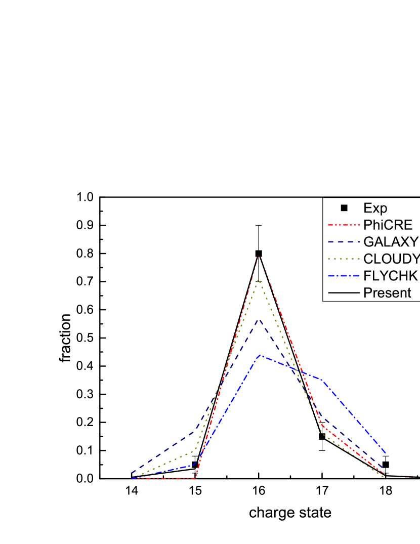
Figure 1: The charge state distribution calculated by RCF (Solid) for Fe photoionization experiment(Scatters), and comparison with PhiCRE (Dash Dot Dot), GALAXY (Dash), CLOUDY (Dot), and FLYCHK (Dash Dot) ([Foord et al.(2006)], [Wang et al.(2011)]). The temperatures are electron temperatures used by these models.

Figure 1 displays the charge state distribution of the iron photoionization experiment predicted by RCF and comparisons with the experiment values and some previous works ([Foord et al.(2006)], [Wang et al.(2011)]). Seemingly, RCF produces the result closest to the experiment, and almost every ion is within the experiment uncertainties. The average charge state in present calculation is $<Z>=16.12$, which agrees well with the measured value $<Z>=16.1\pm 0.2$. The input parameters used here are $T_{r}$=165 eV, $n_{e}=2\times 10^{19}$cm^-3, $\alpha=1.4\%$ and $T_{e}=150eV$. $T_{e}$=150 eV agrees with CLOUDY and FLYCHK, and some other works, such as NIMP ([Rose et al.(2004)]) and Han et al. (2013). $\alpha=1.4\%$ is in the interval deduced above.

A main reason of the differences among the codes in Figure 1 is the different sources of atomic data. GALAXY employs an average-of-configuration approximation for electronic states, screened hydrogenic for both collisional and radiative processes, and Hartree-Dirac-Slater or Kramers cross sections for photoionization ([Rose(1998)], [Foord et al.(2006)]). FLYCHK uses hydrogenic approximation to calculate energy levels and level populations ([Chung et al.(2003)], [Foord et al.(2006)]). Results of GALAXY and FLYCHK largely deviate from the measured one. The atomic databases of CLOUDY are accurate enough to be comparable with spectral emission data ([Ferland et al.(1998)], [Foord et al.(2006)]), but there still are some obvious disparities between it and the experiment. The energy levels and spontaneous decay rates of PhiCRE are taken from the NIST database, and other rate coefficients are calculated by widely used formulas ([Salzmann et al.(2011)], [Wang et al.(2011)]).

The atomic data of RCF are calculated by FAC, which calculates all the atomic data by a fully relativistic approach based on Dirac equation ([Gu(2008)]), and this single theoretical framework ensures self-consistency between different parts. The configurations calculated with FAC of present work are listed Table 3, which include 1948 singly or doubly excited levels. For saving computation time, the maximum principle quantum number n is set to be 4. Because the states with K-shell vacancies have energies higher than 7 keV, which are much higher than the energies of photons and electrons under this experiment condition, K-shell is closed in FAC calculation. For ensuring the accuracy of present work, we compare the present FAC data with some literature values. Table 3 is the comparison of energy levels for $2s^{2}2p^{5}3l$ and $2s2p^{6}3l$ states of Fe¹⁶⁺ between the NIST database ([Kramida et al.(2014)]) and present work, and it shows excellent agreement (within 0.4%). Figure 2 shows the comparison of radiative decay rates (s^-1) between present work and the available corresponding transitions on the NIST database ([Kramida et al.(2014)]) of the four most abundant charge states. As shown, there are more than 80% of present data within 20% agreement with NIST database ([Kramida et al.(2014)]). According to Eq.(14), the accuracy of radiative decay rates also guarantees the calculating of photoexcitation rates. For collisional excitation, Figure 3 is the comparison of cross section of Fe¹⁵⁺ and Fe¹⁶⁺ for transitions from their ground states to their first excited levels. The present FAC results agree well with those calculated with ICFT (intermediate-coupling frame transformation) R-matrix ([Liang et al.(2009)],[Liang & Badnell(2010)]) and Dirac R-matrix ([Aggarwal et al.(2003)]). Using these data, RCF successfully reproduces the experiment result, and we look forward to applying it to spectral analysis of laboratory or astrophysical plasmas in future works.

llllll The configurations used by Case A. Charge State Singly Excited     Doubly Excited  
Charge State Singly Excited     Doubly Excited  
$Fe^{14+}$ $2s^{2}2p^{6}3s^{2}$ $2s^{2}2p^{6}3s3p$ $2s^{2}2p^{6}3p^{2}$ $2s^{2}2p^{5}3s^{2}3p$ $2s2p^{6}3s^{2}3p$
  $2s^{2}2p^{6}3s3d$ $2s^{2}2p^{6}3p3d$ $2s^{2}2p^{6}3d^{2}$    
  $2s^{2}2p^{6}3s4s$ $2s^{2}2p^{6}3s4p$ $2s^{2}2p^{6}3s4d$    
  $2s^{2}2p^{6}3s4f$        
$Fe^{15+}$ $2s^{2}2p^{6}3s$ $2s^{2}2p^{6}3p$ $2s^{2}2p^{6}3d$ $2s^{2}2p^{5}3s^{2}$ $2s^{2}2p^{5}3s3p$
  $2s^{2}2p^{6}4s$ $2s^{2}2p^{6}4p$ $2s^{2}2p^{6}4d$ $2s^{2}2p^{5}3p^{2}$ $2s^{2}2p^{5}3s3d$
  $2s^{2}2p^{6}4f$     $2s^{2}2p^{5}3p3d$ $2s^{2}2p^{5}3d^{2}$
        $2s2p^{6}3s^{2}$ $2s2p^{6}3s3p$
        $2s2p^{6}3p^{2}$ $2s2p^{6}3s3d$
        $2s2p^{6}3p3d$ $2s2p^{6}3d^{2}$
$Fe^{16+}$ $2s^{2}2p^{6}$ $2s^{2}2p^{5}3s$ $2s^{2}2p^{5}3p$ $2s2p^{5}3s^{2}$ $2s2p^{5}3s3p$
  $2s^{2}2p^{5}3d$ $2s2p^{6}3s$ $2s2p^{6}3p$ $2s2p^{5}3p^{2}$ $2s2p^{5}3s3d$
  $2s2p^{6}3d$ $2s^{2}2p^{5}4s$ $2s^{2}2p^{5}4p$ $2s2p^{5}3p3d$ $2s2p^{5}3d^{2}$
  $2s^{2}2p^{5}4d$ $2s^{2}2p^{5}4f$      
$Fe^{17+}$ $2s^{2}2p^{5}$ $2s2p^{6}$ $2s^{2}2^{4}3s$ $2s2p^{4}3s^{2}$ $2s2p^{4}3s3p$
  $2s^{2}2^{4}3p$ $2s^{2}2^{4}3d$ $2s2p^{5}3s$ $2s2p^{4}3p^{2}$ $2s2p^{4}3s3d$
  $2s2p^{5}3p$ $2s2p^{5}3d$ $2s^{2}2^{4}4s$ $2s2p^{4}3p3d$ $2s2p^{4}3d^{2}$
  $2s^{2}2^{4}4p$ $2s^{2}2^{4}4d$ $2s^{2}2^{4}4f$    
  $2s^{2}2^{4}4s$ $2s^{2}2^{4}4p$ $2s^{2}2^{4}4d$    
  $2s^{2}2^{4}4f$        
$Fe^{18+}$ $2s^{2}2p^{4}$ $2s2p^{5}$ $2p^{6}$    
  $2s^{2}2p^{3}3s$ $2s2p^{4}3s$      
$Fe^{19+}$ $2s^{2}3p^{3}$

lllll Comparison of energy levels for $2s^{2}2p^{5}3l$ and $2s2p^{6}3l$ states of Fe¹⁶⁺ between NIST and present work. Index Level   NIST Present
Index Level   NIST Present
0 $2s^{2}2p^{6}$ ${}^{1}S_{0}$ 0 0
1 $2s^{2}2p^{5}3s$ ${}^{3}P_{2}$ 725.2443 723.9074
2   ${}^{1}P_{1}$ 727.1388 725.874
3 $2s^{2}2p^{5}3s$ ${}^{3}P_{0}$ 737.856 736.5231
4   ${}^{3}P_{1}$ 739.0537 737.762
5 $2s^{2}2p^{5}3p$ ${}^{3}S_{1}$ 755.4915 755.008
6 $2s^{2}2p^{5}3p$ ${}^{3}D_{2}$ 758.9928 757.7623
7 ${}^{3}D_{3}$ 760.6095 759.327
8 ${}^{3}D_{1}$ 771.0614 769.7896
9 $2s^{2}2p^{5}3p$ ${}^{1}P_{1}$ 761.7403 760.5093
10 $2s^{2}2p^{5}3p$ ${}^{3}P_{2}$ 763.5529 762.2596
11 ${}^{3}P_{0}$ 768.981 767.8495
12 ${}^{3}P_{1}$ 774.3073 773.1159
13 $2s^{2}2p^{5}3p$ ${}^{1}D_{2}$ 774.6855 773.415
14 $2s^{2}2p^{5}3p$ ${}^{1}S_{0}$ 787.7224 790.3189
15 $2s^{2}2p^{5}3d$ ${}^{3}P_{0}$ 801.4313 800.4122
16 ${}^{3}P_{1}$ 802.401 801.3396
17 ${}^{3}P_{2}$ 804.211 803.0749
18 $2s^{2}2p^{5}3d$ ${}^{3}F_{4}$ 804.2644 802.9189
19 ${}^{3}F_{3}$ 805.0331 803.6367
20 ${}^{3}F_{2}$ 817.5964 816.2671
21 $2s^{2}2p^{5}3d$ ${}^{1}D_{2}$ 806.728 805.3275
22 $2s^{2}2p^{5}3d$ ${}^{3}D_{3}$ 807.8004 806.4032
23 ${}^{3}D_{1}$ 812.369 811.2368
24 ${}^{3}D_{2}$ 818.4135 817.0462
25 $2s^{2}2p^{5}3d$ ${}^{1}F_{3}$ 818.9342 817.4908
26 $2s^{2}2p^{5}3d$ ${}^{1}P_{1}$ 825.7 825.4368
27 $2s2p^{6}3s$ ${}^{1}S_{0}$ 869.1 867.1547
28 $2s2p^{6}3p$ ${}^{3}P_{1}$ 892.55 892.5898
29 $2s2p^{6}3p$ ${}^{1}P_{1}$ 896.939 895.3807

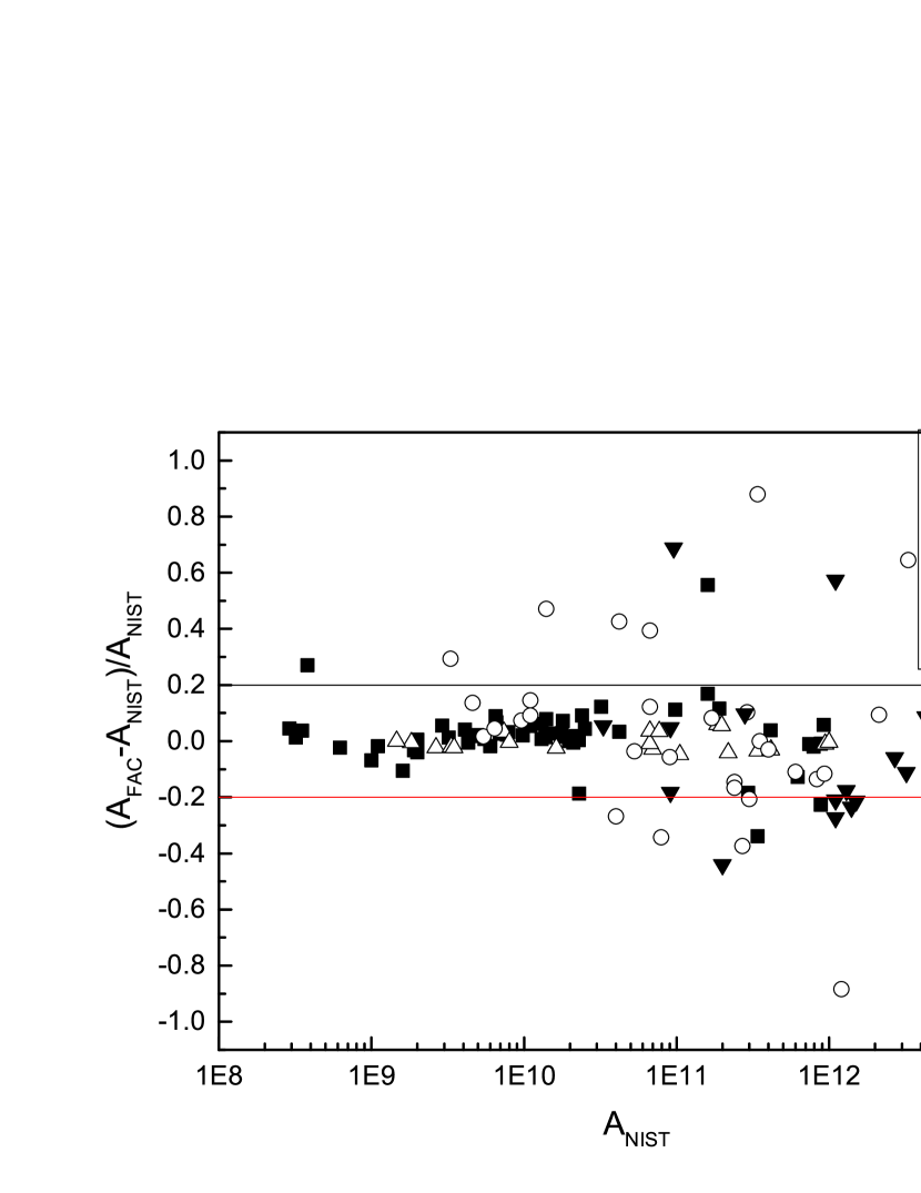
Figure 2: Comparison of radiative decay rates between present work and corresponding available data on NIST from Fe¹⁴⁺ to Fe¹⁷⁺.

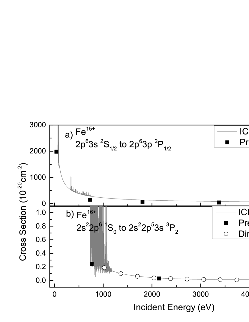
Figure 3: Comparison of collisional excitation cross sections. (a)Transition from $2p^{6}3s$ ${}^{2}S_{1/2}$ to $2p^{6}3p$ ${}^{2}P_{1/2}$ of Fe¹⁵⁺. Grey solid: ICFT R-matrix ([Liang et al.(2009)]), black square: present FAC. (b)Transition from $2s^{2}2p^{6}$ ${}^{1}S_{0}$ to $2s^{2}2p^{5}3s$ ${}^{3}P_{2}$ of Fe¹⁶⁺. Grey solid: ([Liang & Badnell(2010)]), black square: present FAC, circle: Dirac R-matrix ([Aggarwal et al.(2003)]).

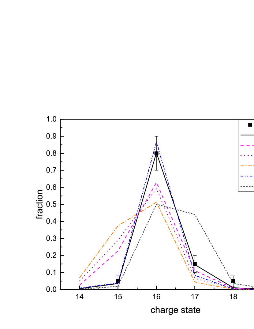
Figure 4: The charge state distribution calculated by RCF with different data or without specific processes. Case A uses data with inner-shell holes (Solid), Case B use data without inner-shell holes (Dash).Case C (Dot), D (Dash Dot), E (Dash Dot Dot) use the same data as Case A, but there are no AI and DC processes in Case C, no PE process in Case D, no PI process in Case E, no CE process in Case F. The scatters are experiment values.

In Figure 4, we compare the influences of some important processes on the experimental results. Case A is the one presented in Figure 1, in which we included all the relevant processes in RCF and all the configurations in Table 3.

Case B uses data without the doubly excited levels in Table 3. As can be seen, there are significant differences relative to Case A.

In Case C both the autoionization and its inverse process, dielectronic capture, are turned off. Results of Case C are close to those of Case B, and both predict an average charge lower than that of Case A. This means that doubly excited states are non-ignorable in the current calculation of charge state distributions. In other words, autoionization is an important ionizing channel, and doubly excited states act like ladders to the next charge state in this experiment.

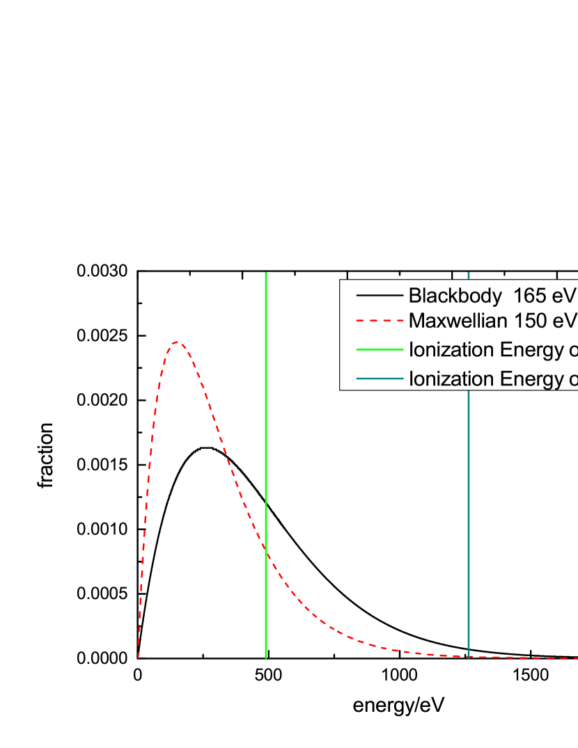
Figure 5: The distribution of 165 eV blackbody photons (solid) and 150 eV Maxwellian electrons (dash).

In Cases D and E, we examine the influence of the radiation field on the Sandia experiment charge state distribution. First we note that there is a big difference between the binding energy of the two most important charge states in the experiment: the ionization energy of Fe¹⁵⁺ (Na-like) is 489.312 eV, and that of Fe¹⁶⁺(Ne-like) is 1262.7 eV. As shown in Figure 5, a larger fraction of photons than electrons has sufficient energy to excite or ionize Fe⁺¹⁵ and Fe⁺¹⁶. In fact, we have found that the influence of electron collisional ionization is so small that its omission from the computations is hardly different from Case A.

There are two radiation driven processes in the code, photoexcitation (PE) and photoionization (PI). PE is omitted in Case D, whereas PI is turned off in Case E. It can be seen from Figure 4 that the absence of PE significantly reduces the average charge state, i.e., photoexcited states play an important role in the charge state distribution. Case E is very close to Case A. The reason for this behavior is the large difference between the binding energies of Fe⁺¹⁵ and Fe⁺¹⁶. On the other hand, there is a threshold between Fe¹⁶⁺ and Fe¹⁷⁺, because neon-like Fe⁺¹⁶ has a closed shell stable configuration.

Both of PE and PI have preference to ionize inner-shell electrons resulting in autoionizing states. However, according to the photon energy distribution in Figure 5 and the energy levels of main ions, the doubly excited levels seem to be more likely produced by PE process. Actually, when the PE channel to doubly excited states is shut down, the result is almost the same as Case D, which confirms that PE is the main pumping mechanism of doubly excited states. Case E indicates that PE+AI process wins the competition in ionizing Fe¹⁵⁺, but for Fe¹⁶⁺ the PI channel is important, too.

In Case F, collisional excitation (CE) is omitted, and it gets a strange result. The deletion of CE does not lower $<Z>$ as Case D, but rather the plasma is more ionized than Case A. According to Figure 5, although the electrons have comparatively lower energy and cannot ionize the ions as effectively as photons, they still can excite the ions to singly excited levels by collision. However, the collision produced singly excited levels have smaller reaction cross sections with photons than the ground state and lower levels, namely, they are more difficult to be ionized by photons. Therefore, the electrons certainly would take part in the competition of reacting with the ground state of ions, and as a result reducing the ionizing efficiency of PI and PE+AI. What is more, when the CE channel from the ground states of ions to the singly excited states is shut down, it produces a result similar to Case F, which confirms the discussion above. So that, it makes sense that why $<Z>$ rises when CE is shut down.

In conclusion, RCF has a good agreement to the photoionization experiment results ([Foord et al.(2004)]), and gives reasonable explanation for the charge state distribution. In the calculations of RCF, the charge state distribution of this experiment is a composite result of different atomic processes. The external field dominates the ionizations in the plasma by photoionization directly and photoexcitation plus autoionization indirectly. The transitions within any given single charge state can significantly affect the charge state distribution, and one of the interesting results of our computations is the role played by collisional excitation in this experiment, in which it reduces the total ionization rate by competing with PE and PI.

4 Summary

In this paper we introduced a new code, RCF, which is applied to plasma in NLTE condition, especially in the photoionization dominating regime. This code can calculate the level population, charge state distribution and spectra of a plasma in steady state. The atomic data source of this code is FAC, which is an easy to use and powerful software package to calculate various atomic data. The SFAC interface can provide all the atomic data needed in RCF, without any additional modifications. FAC is based on a fully relativistic theoretical framework, which ensures the accuracy and consistency of the atomic data.

All the plasma processes and their inverse ones are related by the detailed balance principle in RCF. As a result, in high density regime, the RCF generates results similar to the Saha equation with same atomic data. In other words, RCF converges to LTE approximation under the appropriate condition. In radiation dominant regimes, RCF gets a charge state distribution which closely agrees to the results of the Fe photoionization experiment. A comparison is given to the results of other similar codes. We also discussed the influence of the various atomic processes to the charge state distribution of this experiment. Photoionization is not the only important ionizing channel, but the photoexcitation plus autoionization process are proved to be also significant. Although the electrons have comparatively lower energy than the photons, they still are important. The electrons can excite the ions to the levels which have small reaction cross sections for the photons, and the result is reducing the ionizing efficiency of the photons.

The charge state and levels’ distributions are a prerequisite for the simulation of the emission spectrum, and we showed that all the atomic processes may have significant effect under the appropriate conditions. In particular, in the analysis of X-ray spectrum from a compact object photoexcitation is an important pumping mechanism ([Kallman et al.(2014)]). Porquet & Dubau (2004) also emphasized the influence of cascading decay from higher levels and collisional excitation on the line ratios in plasma diagnosis. According to the result shown, RCF is a reasonable code to get accurate distributions in steady NLTE plasma by including all the processes and using FAC data. We shall use it for spectrum analysis in astrophysics and laboratory of photoionizing and collisional NLTE plasmas in our further works.

Acknowledgement

This work is supported by the NSFC under grants Nos.11173032 and 11135012, and by the National Basic Research Program of China (973 Program) under grant No.2013CBA01503.

References

- [1]
- [Aggarwal et al.(2003)] Aggarwal, K. M., Keenan, F. P., & Msezane, A. Z. 2003, ApJS, 144, 169
- [Bautista & Kallman(2001)] Bautista, M. A., & Kallman, T. R. 2001, ApJS, 134, 139
- [Boroson et al.(2003)] Boroson, B., Vrtilek, S. D., Kallman, T., & Corcoran, M. 2003, ApJ, 592, 516
- [Chung et al.(2003)] Chung, H.-K., Morgan, W. L., & Lee, R. W. 2003, J. Quant. Spec. Radiat. Transf., 81, 107
- [Djaoui & Rose(1992)] Djaoui, A., & Rose, S. J. 1992, Journal of Physics B Atomic Molecular Physics, 25, 2745
- [Ferland et al.(1998)] Ferland, G. J., Korista, K. T., Verner, D. A., et al. 1998, PASP, 110, 761
- [Foord et al.(2004)] Foord, M. E., Heeter, R. F., van Hoof, P. A., et al. 2004, Physical Review Letters, 93, 055002
- [Foord et al.(2006)] Foord, M. E., Heeter, R. F., Chung, H.-K., et al. 2006, J. Quant. Spec. Radiat. Transf., 99, 712
- [Fujioka et al.(2009)] Fujioka, S., Takabe, H., Yamamoto, N., et al. 2009, Nature Physics, 5, 821
- [Gu(2008)] Gu, M. F. 2008, Canadian Journal of Physics, 86, 675
- [Han et al.(2013)] Han, X.-Y., Wang, F.-L., Wu, Z.-Q., Yan, J., & Zhao, G. 2013, Journal of the Physical Society of Japan, 82, 024501
- [Kallman et al.(1996)] Kallman, T. R., Liedahl, D., Osterheld, A., Goldstein, W., & Kahn, S. 1996, ApJ, 465, 994
- [Kallman & Bautista(2001)] Kallman, T., & Bautista, M. 2001, ApJS, 133, 221
- [Kallman et al.(2004)] Kallman, T. R., Palmeri, P., Bautista, M. A., Mendoza, C., & Krolik, J. H. 2004, ApJS, 155, 675
- [Kallman et al.(2014)] Kallman, T., Evans, D. A., Marshall, H., et al. 2014, ApJ, 780, 121
- [Kramida et al.(2014)] Kramida, A., Ralchenko, Yu., Reader, J., and NIST ASD Team (2014). NIST Atomic Spectra Database (ver. 5.2), [Online]. Available: http://physics.nist.gov/asd [2014, November 19]. National Institute of Standards and Technology, Gaithersburg, MD.
- [Liang et al.(2009)] Liang, G. Y., Whiteford, A. D., & Badnell, N. R. 2009, A&A, 500, 1263
- [Liang & Badnell(2010)] Liang, G. Y., & Badnell, N. R. 2010, A&A, 518, AA64
- [Liang et al.(2014)] Liang, G. Y., Li, F., Wang, F. L., et al. 2014, ApJ, 783, 124
- [Porquet & Dubau(2000)] Porquet, D., & Dubau, J. 2000, A&AS, 143, 495
- [Rose(1998)] Rose, S. J. 1998, Journal of Physics B Atomic Molecular Physics, 31, 2129
- [Rose et al.(2004)] Rose, S. J., van Hoof, P. A. M., Jonauskas, V., et al. 2004, Journal of Physics B Atomic Molecular Physics, 37, L337
- [Salzmann(1998)] Salzmann, D. 1998,Atomic Physics in Hot Plasmas(New York:Oxford Univ.Press)
- [Salzmann et al.(2011)] Salzmann, D., Takabe, H., Wang, F., & Zhao, G. 2011, ApJ, 742, 52
- [Wang et al.(2011)] Wang, F., Salzmann, D., Zhao, G., & Takabe, H. 2011, ApJ, 742, 53