Toward Fast Topological-Shape Optimization With Boundary Elements

Abstract

Abstract. Wide variety of engineering design tasks can be formulated as constrained optimization problems where the shape and topology of the domain are optimized to reduce costs while satisfying certain constraints. Several mathematical approaches were developed to address the problem of finding optimal design of an engineered structure. Recent works [1, 2] have demonstrated the feasibility of boundary element method as a tool for topological-shape optimization. However, it was noted that the approach has certain drawbacks, and in particular high computational cost of the iterative optimization process. In this short note we suggest ways to address critical limitations of boundary element method as a tool for topological-shape optimization. We validate our approaches by supplementing the existing complex variables boundary element code for elastostatic problems with robust tools for fast topological-shape optimization. The efficiency of the approach is illustrated with a numerical example.

1 Introduction

Problems of optimal design, i.e. variation of shape and topology of the domain to extremize certain functional subject to additional constraints, are ubiquitous in different branches of engineering. Recent emergence and rapid development of stereolithography and 3D printing technologies [3, 4] have enabled fast prototyping of complex-shaped structures and revived the interest in automated optimal design. The most common formulation of optimization problems studied in structural engineering (e.g. [5]) seeks for an optimal shape and topology of an elastic body that minimize the strain energy (compliance) while satisfying the weight constraint and the additional constraints imposed by the boundary value problem. Non-convex nature of such optimization problems often makes finding globally optimal designs difficult or impossible. Various numerical methods, including shape gradient-based approaches [6], level set methods [7, 8], homogenization [9, 10] and topological-shape sensitivity [11] have been developed during the last few decades to address this class of problems. These approaches are typically implemented within the finite element method (FEM) context. In case if admissible designs include only homogeneous regions with piecewise-constant properties (micro-structured composite designs are prohibited), the problem of optimization reduces to finding optimal configuration of the domain boundaries. Few recent papers [1, 2] suggested that boundary integral approaches, and in particular boundary element method (BEM), can be a convenient tool to address this class of problems. The implementation of optimization algorithms within BEM utilizes the concept of topological derivative (TD) [12, 11, 13] - a cost of making an infinitesimal circular (spherical) cavity with a center in a given point of the domain. Existence of this kind of derivative opens wide avenue for numerous gradient-based approaches. The most straightforward one utilizes the idea of calculation of the field of TD on a given mesh, and removing material in the regions where the TD is below certain cutoff level. This kind of approach has demonstrated its feasibility in both 2D and 3D elastostatic problems [1, 2]. However, existing papers on the subject do not address the issue of complexity of topological-shape optimization with BEM, and, particularly, the question of competitiveness of BEM approaches as compared to FEM.

In this note we suggest a simple optimization technique based on 2D BEM. It is demonstrated that even without using fast BEM techniques, one can easily reach $O(n_{s}^{2})$ asymptotic performance of shape optimization with BEM, which corresponds to the performance of 2D FEM approaches - $O(n_{v})$ ($n_{s}$ and $n_{v}$ are the numbers of surface elements and volume elements after BEM/FEM discretization).

The suggested technique is based on complex variables boundary element method (CVBEM) [14]. It utilizes quadtree-based calculation of TD inside the domain, allowing $O(n_{s}^{2})$ performance of evaluation of fields inside the domain. We also use simple $O(n_{s}^{2})$ algebraic solver based on blockwise update of the inverse system matrix to solve direct boundary value problem at every iteration.

The paper has the following organization. The next section describes the method of topological optimization employed in our research, as well as its novel features. Section 3 provides an illustrative numerical example that is served to highlight the capabilities of our approach. The summary and discussion of our results, as well as the major directions of future work are presented in Section 4.

2 Method

2.1 Optimization technique

In this paper we develop our approach in 2D using the framework of CVBEM [14]. The method offers a number of attractive features: i) complex hypersingular boundary integral equation (BIE) for tractions and displacement discontinuities, derived for a system that can include an infinite matrix, finite-sized blocks with piecewise-constant properties, voids and cracks [14]; ii) closed form analytical calculation of all the integrals in BIE [14], iii) circular elements to approximate curved boundaries [14]; vi) asymptotic approximations to model cracks [14]; v) implementation of piecewise-constant body forces [15].

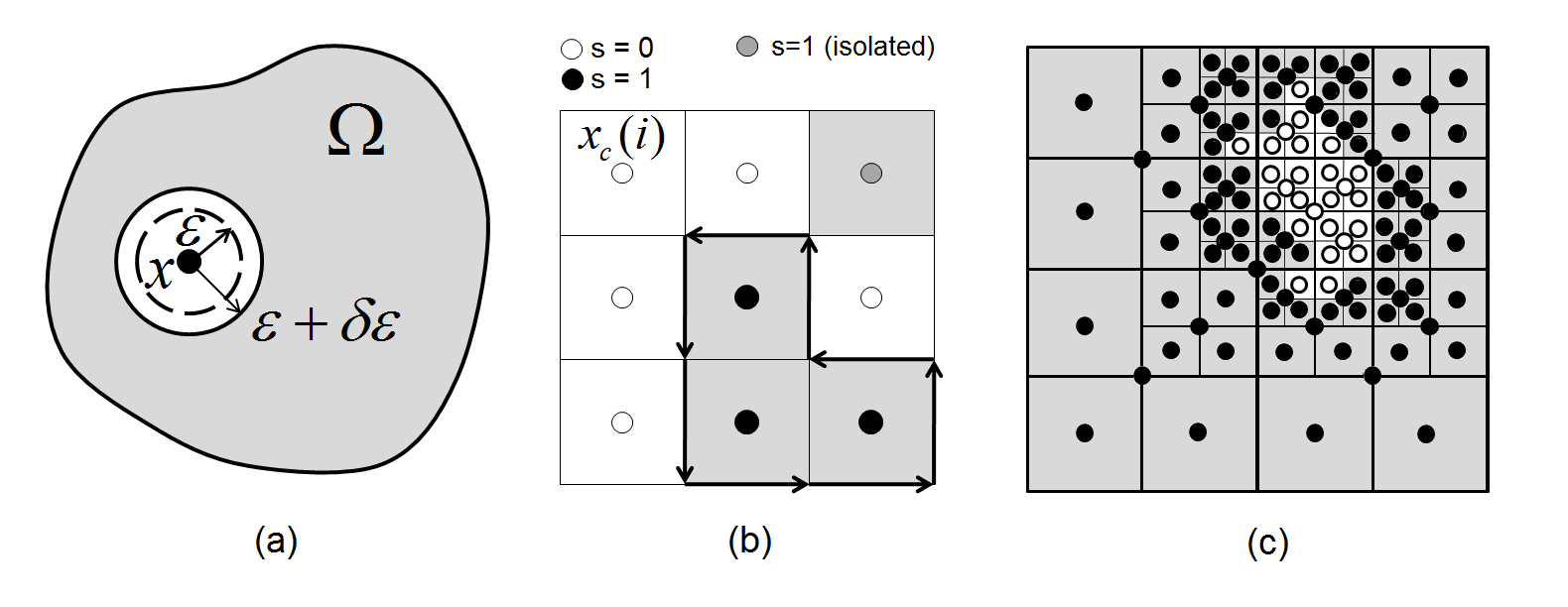
Figure 1: (a) Details on the definition of TD. (b) Optimization on the rectangular mesh. (c) Quadtree strategy of sampling of the TD inside the domain.

Our scheme of topological optimization utilizes the notion of topological derivative [11]. Following [16] we define the TD as (Fig. 1(a)):

$$D(x)=\underset{\underset{\delta\varepsilon\rightarrow 0}{\varepsilon\rightarrow 0}}{\lim}\frac{\varPsi(\varOmega_{\varepsilon+\delta\varepsilon})-\varPsi(\varOmega_{\varepsilon})}{f(\varepsilon+\delta\varepsilon)-f(\varepsilon)}$$ (1)

Here $\Psi$ is the cost functional, $\Omega_{\varepsilon}$ is the original domain perturbed by the presence of an infinitesimal cavity of radius $\varepsilon$ centered at the point $x$, $\delta\varepsilon$ is the small perturbation of the cavity radius, and $f$ is regularizing, problem-dependent function. Here and below we’ll be working with the strain energy functional, that serves as a global measure of compliance of an elastic structure. For this case the area (volume) of the cavity serves as regularizing function. In absence of body forces, the closed form analytical expressions are available both in 2D and 3D [16, 5]. In the case of 2D plane strain elasticity the expression for TD writes

$$D(x)=\frac{2}{(1+\nu)(1-2\nu)}\sigma\cdot\epsilon+\frac{(1-\nu)(4\nu-1)}{2(1-2\nu)}tr\sigma tr\epsilon$$ (2)

Here $\sigma$ and $\epsilon$ are stress and strain tensors at point $x$. In case of presence of a constant body force $\boldsymbol{b}$ the expression (2) should be enriched with an additional term, associated with work done by the body force $-\boldsymbol{bu}(x)$, where $\boldsymbol{u}(x)$ is displacement at point $x$. The treatment of constant body force within CVBEM is discussed in [15]. It worth noting here that similar analytical expressions for TDs are also available for other important classes of cost functionals, in particular, for the components of homogenized elasticity tensor of a periodic cell [17, 18].

Shape optimization approaches based on TDs use either hard-kill methods [16, 1], or bidirectional optimization[19]. In our work we utilize a hard-kill algorithm, in which the optimization is achieved by progressive elimination of material in the areas where the TD is below the cutoff level, as discussed further.

2.2 Boundary generation procedure

The new set of domain boundaries is created at every iteration of optimization procedure. Boundary generation strategy employed in our work is similar to one described in [2]. We discretize the initial domain onto a set of $M$ square cells (Fig. 1(b)). The fields inside the domain are calculated at the center of each cell $x_{c}(i)$, $i=1..M$. The cutoff level for the TD is defined as $D_{0}=D_{min}+\alpha(D_{max}-D_{min})$, where $D_{min}$ and $D_{max}$ are minimum and maximum values of TD within the current domain, and the coefficient $\alpha$ is tuned in range between 0.1% and 2%. For every cell of the initial domain we define the Boolean status $s$. At the beginning of the iterative process $s=1$ for every cell. At every iteration we assign $s=0$ for the cells with $D(x_{c}(i))<D_{0}$ (marked with empty points in Fig. 1(b)), and for isolated cells (marked with gray points in Fig. 1(b)). When the status is assigned, we generate the new boundary using straightforward algorithm - if $i$-th cell has $s=1$ and its right (top, left, bottom) neighbor has $s=0$, then generate a corresponding boundary element. For every boundary between the neighboring cells one straight element with three points of collocation (quadratic approximation) is used. At every iteration we mark the elements that were deleted and those that were added at the current step.

Boundary value problem constraints are incorporated explicitly - for the cells bounded by the elements with non-homogeneous Neumann boundary conditions $s\equiv 1$. The volume constraint does not present explicity in this scheme, so it is incorporated as the stopping criteria - the iterative process is discontinued when the ratio of current area of the material to the initial one $R$ reaches the prescribed value $R_{0}$.

2.3 Quadtree sampling of fields inside the domain

The described procedure of sampling of TDs on the uniform mesh should be considered computationally inefficient, since the calculation of a field of TDs inside the domain takes $O(n_{s}^{3})$ operations. In order to reduce the asymptotic complexity of this step, we use the specific strategy of calculation of TDs, which is based on quadtree algorithm of sampling [20]. The main idea is to use few different levels of refinement, that are employed for initial detection and further refinement of features of optimized domain. Within this approach each refined cell is subdivided onto 4 sub-cells (Fig. 1(c)). One can formulate different possible criteria of refinement. In this work we use the following criterion - if the values of $s$ for a current cell and its nearest neighbor are not the same, both cells should be refined to the next level. The boundary generation algorithm described above is used to generate boundaries around the points of highest level of refinement. It is easy to see that such an algorithm of sampling and boundary generation requires calculation of the topological derivative at $O(n_{s})$ points inside the domain, leading to $O(n_{s}^{2})$ operations of evaluations of boundary integrals for each boundary element.

2.4 Iterative update of the inverse matrix

CVBEM [14] generates non-symmetric and non-sparce system matrix, and the corresponding system of equations is difficult to solve using regular iterative approaches. Here we describe one possible way to treat the resulting system matrix during the iterative updates of the initial boundary value problem. The original boundary consisting of $n_{s}$ elements leads to $N_{s}=6n_{s}$ rows/columns in the resulting non-symmetric matrix generated by CVBEM (considering $3$ collocation points per element and $2$ degrees of freedom per collocation point). Assume that at $k-th$ iteration $n_{a}$ elements have been added to a boundary, and $n_{r}$ elements have been removed. This results in $N_{a}=6n_{a}$ and $N_{r}=6n_{r}$ added and removed rows/columns in the system matrix. If, as always the case in the iterative process, $n_{a}\ll n_{s}$, $n_{r}\ll n_{s}$, it is efficient to perform update of the inverse matrix using incremental expressions, such as Sherman–Morrison–Woodbury formula [21] or Banachiewicz [22] formula for blockwise matrix inverse:

$$\left(\begin{array}[]{cc}A&B\\ C&D\end{array}\right)^{-1}=\left(\begin{array}[]{cc}A^{-1}+A^{-1}BS{}^{-1}CA^{-1}&-A^{-1}BS{}^{-1}\\ -S^{-1}CA^{-1}&S^{-1}\end{array}\right)$$ (3)

Where $S=D-CA^{-1}B$. Denoting blocks of an extended matrix as $E,F,G$ and $H$, and expressing $A^{-1}$, we obtain the formula for inverse matrix update in case of removing elements:

$$A^{-1}=\left(\begin{array}[]{cc}E&\cancel{F}\\ \cancel{G}&\cancel{H}\end{array}\right)^{-1}=E-FH^{-1}G$$ (4)

It is clear that calculations of both expressions do not require $(N_{s}\times N_{s})(N_{s}\times N_{s})$ matrix multiplications, only lower-rank operations with $(N_{s}\times N_{s})$, $(N_{s}\times N_{a})$,$(N_{s}\times N_{d})$,$(N_{a}\times N_{a})$ and $(N_{d}\times N_{d})$ matrices. This leads to $O(n_{s}^{2})$ performance of the algorithm of iterative matrix update.

It is important to mention that in case if the matrix update is associated with the new cavity in the domain, matrix $S$ is singular and requires regularization, e.g. truncated SVD regularization [23] (used in this work) or explicit incorporation of additional conditions that fix rigid body motion of a new closed boundary [14].

The suggested (or similar) schemes of low-rank inverse matrix update are well know and are widely used in adjacent fields of scientific and engineering calculations, including network structures, asymptotic analysis and boundary value problems with changing boundaries (see the excellent review presented in [24]). It is thus natural to adopt this approach for fast iterative optimization schemes with boundary elements.

3 Numerical example

In this section we discuss a simple benchmark example that allows us to evaluate the capabilities of our approach. Consider a 2D problem of optimization of a shape and topology of a fixed support. The initial domain has the square shape (Fig. 2(a)). The left side of the support is rigidly fixed, and the point load is applied at the upper-right angle.

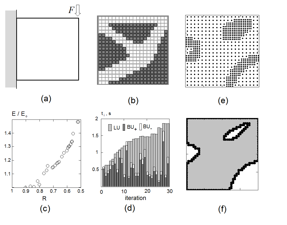
Figure 2: Shape optimization of a fixed support. (a) Initial boundary value problem. (b) Final configuration reached after $29$ iterations. (c) The ratio of current strain energy $E$ to the initial strain energy $E_{0}$ as a function of current volume fraction $R$.

We utilize the optimization scheme described above to find an optimal shape and topology of the support, providing the smallest strain energy $E$ for the volume fraction $R_{0}=0.5$. The cutoff parameter $\alpha$ was set to $0.003$. The TDs are sampled on a grid containing $20\times 20$ cells. The solution was found in $29$ iterations. The final shape is given in Fig. 2(b). The obtained solution is in good agreement with the one obtained with FEM and BEM in the earlier works [16, 1]. Fig. 2(c) gives the evolution of the strain energy functional during the iterative process. Fig. 2(d) presents the comparison of times spent during the iteration with full LU factorization ($LU$), and the blockwise inverse matrix update, including adding rows/columns according to (3) ($BU_{+}$) and removing rows/columns according to (4) ($BU_{-}$). The boost in performance clearly depends on rank of the update (number of added/removed elements) and varies significantly from iteration to iteration. The total time spent on the full LU factorization is 41 s, whereas the total time spent on the blockwise matrix update is 15.5 s. Calculations were performed with regular Core i-5 laptop machine. Linear algebra operations were implemented within non-optimized BLAS/LAPACK framework [25] and win-32 gfortran compiler [26].

In order to illustrate the quadtree sampling of TDs inside the domain, we consider the same example, but with the twice higher degree of grid refinement. Two levels of grid refinement are used. The coarse level discretizes domain onto $20\times 20$ cells. As we could see above, this level is sufficient to detect the important features of the optimized domain. On the finer level we discretize the domain onto $40\times 40$ cells. This level is used to render finer features of the optimal design. Fig. 2(e) gives the sampling points during first iteration, Fig. 2(f) demonstrates corresponding configuration of domain boundaries. Using quadtree sampling has led to decrease of the number of points inside the domain from 1600 to 676, and decrease of the corresponding computational time from 11.3 to 4.8 s.

4 Discussion and conclusions

In this work we suggested a set of tools for topological-shape optimization with boundary elements. As we could see on the example of 2D CVBEM method and a simple toolkit for topological optimization, one can reach the computational performance available with 2D FEM techniques.

It is therefore clear that the usage of fast BEM techniques [27, 28] would undoubtedly allow to outperform all the existing FEM techniques of topological-shape optimization. For example, using fast BEM would allow solution of direct boundary value problem for $O(n_{s})$ operations, and calculation of the field of TD inside the domain for $O(n_{s}ln(n_{s}))$ operations, which is much faster than the corresponding operations performed within FEM (both take $O(n_{v})$ operations). In addition, FEM techniques require good quality domain discretization, generation of which takes at least $O(n_{v}ln(n_{v}))$ operations.

These considerations motivate the development of three-dimensional fast BEM-based framework for topological-shape optimization of an elastic domain. Its implementation can be based on the principles similar to those presented in this work, and extended with additional features: smoother boundaries generation, combined shape and topology optimization iterations, etc. Clearly, the BEM-based techniques should become the most computationally efficient tools for topological-shape optimization.

References

- [1] Marczak, R., 2007. “Optimization of elastic structures using boundary element and a topological-shape sensitivity formulation”. In Mechanics of Solids in Brazil. Brasilian Society of Mechanical Sciences and Engineering, pp. 279–293.
- [2] Bertsch, C., Cisilino, A., Langer, S., and Reese, S., 2008. “Topology optimization of 3d elastic structures using boundary elements”. In Proc. Appl. Math. Mech. 8, pp. 10771–10772.
- [3] Gross, B., Erkal, J., Lockwood, S., Chen, C., and Spence, D., 2014. “An evaluation of 3d printing and its potential impact on biotechnology and the chemical sciences”. Analytical Chemistry, 86(7), pp. 3240–3253.
- [4] Melchels, F. P. W., Feijen, J., and Grijpma, D. W., 2010. “A review on stereolithography and its applications in biomedical engineering”. Biomaterials, 31(24), pp. 6121–6130.
- [5] Novotny, A., Feijoo, R., Taroco, E., and Padra, C., 2007. “Topological sensitivity analysis for three-dimensional linear elasticity problem”. Computational Methods in Applied Mechanics and Engineering(196), pp. 4354–4364.
- [6] Azegami, H., Shimoda, M., Katamine, E., and Wu, Z., 1995. “A domain optimization technique for elliptic boundary value problems”. In Computer Aided Optimization Design of Structures IV, Structural Optimization, S. Hernandez, M. El-Sayed, and C. Brebbia, eds. Computational Mechanics Publications, Southampton.
- [7] Allaire, G., Jouve, F., and Toader, A.-M., 2004. “Structural optimization using sensitivity analysis and a level-set method”. Journal of Computational Physics, 194(1), pp. 363–393.
- [8] Amstutz, S., and Andra, H., 2006. “New algorithm for topology optimization using a level-set method”. Journal of Computational Physics, 216(2), pp. 573–588.
- [9] K.Suzuki, and Kikuchi, N., 1991. “A homogenization method for shape and topology optimization”. Computer methods in applied mechanics and engineeirng, 93, pp. 291–318.
- [10] Allaire, G., Bonnetier, E., Francfort, G., and Jouve, F., 1997. “Shape optimization by the homogenization method”. Numerische Mathematik, pp. 27–68.
- [11] Novotny, A., and Sokolovsky, J., 2013. Topological Derivatives in Shape Optimization. Springer Heidelberg New York Dordrecht London.
- [12] Sokolovski, J., and Zochovski, A., 1999. “On topological derivative in shape optimization”. SIAM Journal on Control and Optimization, 37(4), pp. 1251–1272.
- [13] Sokolovski, J., and Zochovski, A., 2002. “Topological derivatives of shape functionals for elasticity systems”. ISNM International Series of Numerical Mathematics, 139, pp. 231–244.
- [14] Mogilevskaya, S., 1996. “The universal algorithm based on complex hypersingular integral equation to solve plane elasticity problems”. Computational Mechanics, 18, pp. 127–138.
- [15] Ostanin, I., Mogilevskaya, S., Labuz, J., and Napier, J., 2011. “Complex variables boundary element method for elasticity problems with constant body force”. Engineering Analysis with Boundary Elements, 35(4), pp. 623–630.
- [16] Feijoo, R. A., Novotny, A. A., Padra, C., and Taroco, E. O., 2002. “The topological-shape sensitivity analysis and its applications in optimal design”. Mecanica Computacional, XXI, pp. 2687–2711.
- [17] Barbarosie, C., and Toader, A.-M., 2010. “Shape and topology optimization for periodic problems. part i: The shape and the topological derivative”. Structural and Multidisciplinary Optimization, 40, pp. 381–391.
- [18] Barbarosie, C., and Toader, A.-M., 2008. “Shape and topology optimization for periodic problems. part ii: Optimization algorithm and numerical examples”. Preprint CMAF, 017, pp. 1–14.
- [19] Querin, O., Steven, G., and Xie, Y., 1998. “Evolutionary structural optimisation (eso) using a bidirectional algorithm”. Engineering Computations, 15(8), pp. 1031–1048.
- [20] Finkel, R. A., and Bentley, J., 1974. “Quad trees a data structure for retrieval on composite keys”. Acta Informatica, 4(1), pp. 1–9.
- [21] Duncan, W., 1944. “Some devices for the solution of large sets of simultaneous equations (with an appendix on the reciprocation of partitioned matrices)”. The London, Edinburgh and Dublin Philosophical Magazine and Journal of Science, 7(35), p. 660.
- [22] Banachiewicz, T., 1937. “Zur berechnung der determinanten, wie auch der inversen, und zur darauf basierten auflosung der systeme linearer gleichungen.”. Acta Astronomica, c(3), pp. 41–67.
- [23] Hansen, P. C., 1987. “The truncated svd as a method for regularization”. BIT Numerical Mathematics, 27(4), pp. 534–553.
- [24] Hager, W., 1989. “Updating the inverse of a matrix”. SIAM Review, 31(2), pp. 221–239.
- [25] Anderson, E., Bai, Z., Bischof, C., Blackford, S., Demmel, J., Dongarra, J., Du Croz, J., Greenbaum, A., Hammarling, S., McKenney, A., and Sorensen, D., 1999. LAPACK Users’ Guide, third ed. Society for Industrial and Applied Mathematics, Philadelphia, PA.
- [26] Free Software Foundation, I., 2014.
- [27] Nishimura, N., 2002. “Fast multipole accelerated boundary integral equation methods”. Applied Mechanics Reviews, 55(4), pp. 299–324.
- [28] Benedetti, I., Aliabadi, M., and Davi, G., 2008. “A fast 3d dual boundary element method based on hierarchical matrices”. International Journal of Solids and Structures, 45, pp. 2355–2376.