Homogeneous spectroscopic parameters for bright planet host stars from the northern hemisphere

Abstract

Aims. In this work we derive new precise and homogeneous parameters for 37 stars with planets. For this purpose, we analyze high resolution spectra obtained by the NARVAL spectrograph for a sample composed of bright planet host stars in the northern hemisphere. The new parameters are included in the SWEET-Cat online catalogue.

Methods. To ensure that the catalogue is homogeneous, we use our standard spectroscopic analysis procedure, ARES+MOOG, to derive effective temperatures, surface gravities, and metallicities. These spectroscopic stellar parameters are then used as input to compute the stellar mass and radius, which are fundamental for the derivation of the planetary mass and radius.

Results. We show that the spectroscopic parameters, masses, and radii are generally in good agreement with the values available in online databases of exoplanets. There are some exceptions, especially for the evolved stars. These are analyzed in detail focusing on the effect of the stellar mass on the derived planetary mass.

Conclusions. We conclude that the stellar mass estimations for giant stars should be managed with extreme caution when using them to compute the planetary masses. We report examples within this sample where the differences in planetary mass can be as high as 100% in the most extreme cases.

1 Introduction

The stellar characterization of planet hosts is fundamental and has a direct impact on the derivation of the bulk properties of exoplanets. Moreover, it provides unique evidence for the understanding of planet formation and evolution. One early indication was that the giant exoplanets were preferentially discovered orbiting metal-rich stars (Gonzalez, 1997; Santos et al., 2000, 2004; Fischer & Valenti, 2005; Sousa et al., 2008). Later, it was also observed that this metallicity correlation is not the same for less massive planets (Sousa et al., 2011b; Mayor et al., 2011; Buchhave et al., 2012). This evidence give strength to the theory of core-accretion for the planet formation (e.g., Mordasini et al., 2009, 2012). We note, however, that although these correlations seem to be clear for dwarf stars, the same scenario is not so clear for evolved giant stars (e.g., Maldonado et al., 2013; Mortier et al., 2013). Interestingly, the stellar metallicity plays a crucial role not only on planet formation, but also on the evolution and architecture of the planetary systems. For instance, Beaugé & Nesvorný (2013) and Adibekyan et al. (2013) found that planets around metal-poor stars show longer periods, and probably migrate less.

These are just a few of the many examples revealing the importance of stellar characterization for the study of planetary systems. One fundamental aspect common to many of these studies is the homogeneity of methods used to characterize the stars. With this in mind, the SWEET-Cat (Santos et al. 2013) catalogue is available to the community with a very ambitious objective: to provide homogeneous spectroscopic parameters for all planet hosts detected with radial velocity, astrometry, and transit techniques. In this work we focus our attention on the bright northern hemisphere targets that were significantly lacking in this catalogue, and therefore we increase the number of these planet hosts with homogeneous spectroscopic parameters (84% to 93% for all known RV planet host stars known at the present time).

2 Data

The stars analyzed in this work were selected in order to extend the SWEET-CAT catalogue with missing homogeneous parameters. In order to save telescope time, we only focused on northern brighter planet host stars (V ¡ 9 and $\delta>+30\textordmasculine$) for which there were not any suitable spectra available in any high resolution spectrograph archive.

The spectroscopic data were collected between 16 April 2013 and 20 August 2013 with the NARVAL spectrograph located at the 2-meter Bernard Lyot Telescope (@ Pic du Midi). The data was obtained through the Opticon proposal (OPTICON_2013A_027). The spectra were collected in “spectroscopic/object only” mode which allows us to have a high resolution of R $\sim$ 80 000. The exposure times for the stars were chosen in order to reach high signal-to-noise ratio for all the targets ($\geq$ 200). The spectra were reduced using the data reduction software Libre-ESpRIT (Donati et al., 1997) from IRAP (Observatoire Midi-Pyrénées).

The star HD 132563B was observed at two epochs with low signal-to-noise. These two spectra were combined in order to increase the signal-to-noise for this star. This was achieved using the scombine routine which is part of IRAF .

3 Spectroscopic parameters

3.1 Spectroscopic analysis

To derive homogeneous spectroscopic parameters for SWEET-Cat, we made use of our standard spectroscopic analysis (ARES+MOOG; see Sousa et al., 2008; Molenda-Żakowicz et al., 2013; Sousa, 2014). In summary, the measurement of the equivalent widths (EWs) was done automatically and systematically using the ARES code (Sousa et al., 2007). The EWs were then used together with a grid of Kurucz Atlas 9 plane-parallel model atmospheres (Kurucz, 1993). The abundances were computed using MOOG. For the analysis, we first used the linelist from Sousa et al. (2008). However, since a large number of the planet hosts turned out to be cool K stars, we reanalyzed the stars with temperatures lower than 5200 K with a recent linelist from Tsantaki et al. (2013).

During the analysis we identified three planet hosts for which we were not able to derive reliable parameters with ARES+MOOG. Two of them (HD 8673 and XO-3) revealed a significant high rotational velocity, making the measurement of the individual equivalent widths difficult. For these cases the use of a new analysis based on a synthesis method is presented in Tsantaki et al. (2014).

The third planet host for which we were not able to have reliable results with ARES+MOOG is HD 208527, marked as a K5V star in SIMBAD, but which is actually an M giant star (Lee et al., 2013). The problem is also connected with the difficulty of measuring equivalent widths. Here we also have strongly blended lines due to the presence of many more spectral lines, including those from molecular species.

Table 11 presents the spectroscopic parameters derived with ARES+MOOG. The errors were determined following the same procedure as in previous works (Santos et al., 2004; Sousa et al., 2008, 2011b).

We would also like to note that three stars in our sample were already analyzed in the SWEET-Cat catalogue with the same procedure but using other spectroscopic data, allowing us to check the consistency of our results. The stars HD 118203 and HD 16175 were analyzed in Santos et al. (2013) using spectra from SARG and FIES, respectively, while HD 222155 was analyzed in the work of Boisse et al. (2012) using spectra from the SOPHIE spectrograph. Our results are consistent with those previously obtained with other spectrographs.

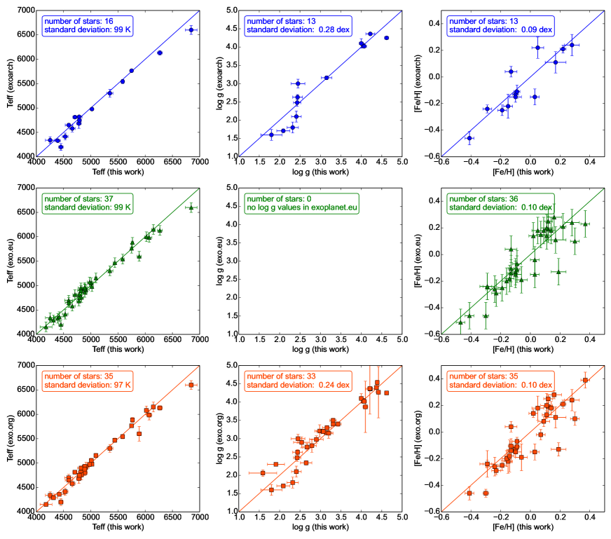
Figure 1: Comparison of the spectroscopic stellar parameters (Teff - left panels; log g - middle panels; [Fe/H] - right panels) derived in this work with the ones that are available in exoarch (top row - red circles), exo.eu (middle row - green triangles), and exo.org (bottom row - orange squares). The comparison shows general good consistency, but reveals some outliers that are discussed in the text.

3.2 Comparison with literature

To perform a comparison with values of spectroscopic parameters derived in other works we used the following online catalogues to collect the data: the Extrasolar Planets Encyclopaedia (hereafter exo.eu; Schneider et al., 2011), the exoplanets.org (here after exo.org; Wright et al., 2011), and the NASA Exoplanet Archive(here after exoarch).

Figure 1 shows the comparisons of the effective temperature, surface gravity, and metallicity for the stars in common between each of the catalogues and our sample. For both the exo.eu and exo.org we were able to find parameters for almost all the stars in our sample, while for the exoarch we have fewer stars with parameters available for the comparison. We note that for the case of exo.eu we do not have the stellar log g available.

The comparisons are generally quite consistent for the temperatures, surface gravities, and metallicities, with standard deviations of the differences around 100 K, 0.25 dex, and 0.1 dex, respectively. The significant high dispersion certainly comes from the heterogeneous nature of the literature compilations.

There are three stars in the comparison with significant large differences in effective temperature (see Fig. 1). These are the cases of 42 Dra, HAT-P-14, and HD 118203. Interestingly, these stars have very different temperatures covering different spectral types.

42 Dra:

This is a K giant star and in both the exo.eu and exoarch catalogues the provided temperature is 4200 K (Döllinger et al., 2009), which is a difference of about 250 K with the one derived in this work (4452 K). Using the VizieR database, we found a dispersion of temperatures for this star between 4200 K to 4500 K. We note that most of the temperatures in VizieR for this star fall in the range 4400-4500 K, which is in good agreement with our measurement.

HAT-P-14:

This is a F dwarf star, and actually the hottest star in the sample, appearing in the top-right corner of the left panels in Fig. 1. The difference is again nearly 250 K (6845 K being our value against the 6600 K found in the online databases). Making a new census using VizieR to find additional temperatures for this star, we found only a few values ranging from 6427 K to 6671 K. Our value is still compatible with the higher values found when considering the errors.

HD 118203:

This is a star much more similar to our Sun. However, when comparing it with the exoplanet databases the difference is surprisingly large, almost 300 K (5890 K being our value against the 5600 K found in the online databases). The values that we found in the literature, again using VizieR, vary from 5600 K up to 5910 K. Given that our analysis is actually a differential analysis relative to the Sun (Sousa et al., 2008; Sousa, 2014), we are very confident in our temperature derivation for this star.

For the surface gravity the comparisons are quite consistent, with larger dispersion for the giant stars (surface gravity lower than 2.5 dex), but without a clear outlier that deserves to be discussed. The good consistency in surface gravity for giants is in line with our latest results (Mortier et al., 2014).

The dispersion in metallicity is quite significant, but HD 139357 clearly stands out as an outlier showing a difference of more than 0.3 dex between the values that we found on exo.eu and exo.org (-0.13 dex in both cases) and the value derived in this work (0.19 dex). As before, using VizieR to find additional values in the literature, we found values ranging from -0.13 dex up to as much as 0.34 dex. Such differences in metallicity might indeed significantly affect the stellar mass estimation and consequently the mass of the planet (see Sect. 4.4 for a deeper discussion of this particular case).

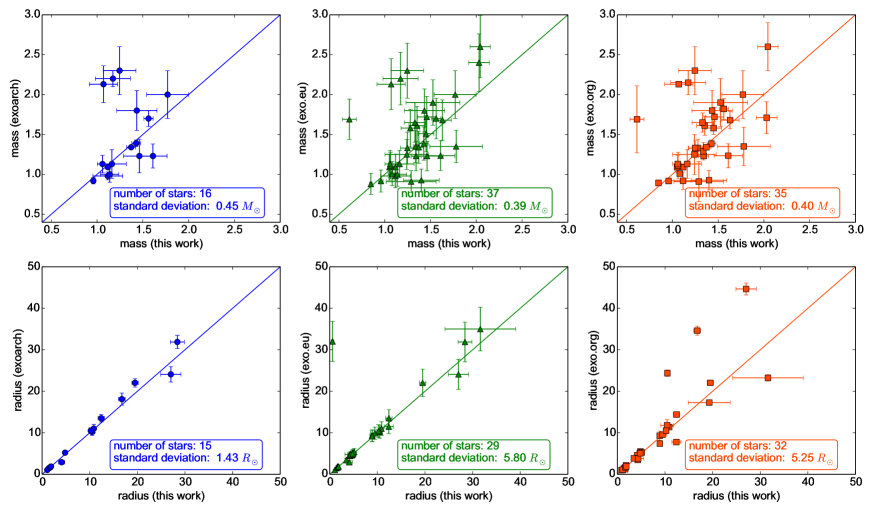
Figure 2: Comparison of the stellar masses (top row) and stellar radius (bottom row) estimated in this work with the ones that are available in exoarch (left column - red circles), exo.eu (middle column - green triangles), and exo.org (right column - orange squares). The comparison reveals some extreme outliers that are discussed in detail in the text.

4 Stellar masses

4.1 Methods used to estimate the stellar mass

To estimate the mass for these planet host stars in a homogeneous way we follow the same procedure that was used in SWEET-CAT (see Santos et al., 2013). Because most of the planet hosts analyzed here are evolved stars, we used the web interface for the Bayesian estimation of stellar parameters based on the PARSEC isochrones (da Silva et al., 2006; Bressan et al., 2012). This web interface also derives an estimation for the stellar radius and the age. To use this tool we need the parallax values for the stars. These were compiled from the SIMBAD astronomical database whenever they were present. For the cases where the parallax value is not available, we computed the spectroscopic parallax using our derived spectroscopic stellar parameters (for more details on the iterative method see Sousa et al. (2011a)).

To double check the results from this iterative method we computed the spectroscopic parallax (and iterative mass) for all the stars analyzed in this work. The comparison for the stars that have parallax present in SIMBAD can be seen in Fig. 3. The top panel shows a direct comparison between the parallax values showing a dispersion with a standard deviation of 2 milliarcseconds. The bottom plot of the same figure shows the comparison of the masses computed using the different parallax values. As already shown in Sousa et al. (2011a), the comparison is in general agreement with a significant large dispersion on the masses. The standard deviation here has a value of 0.22 $M_{\sun}$. We note that a few stars (4 UMa, HD 116029, HD 139357, HD 173416, and HD 240237) show a significant difference in the mass determinations by the two methods, thus heavily contributing to the large dispersion. If we remove these five stars from the comparison, then the standard deviation drops to 0.09 solar masses, which is compatible with the previously observed result (Sousa et al., 2011a).

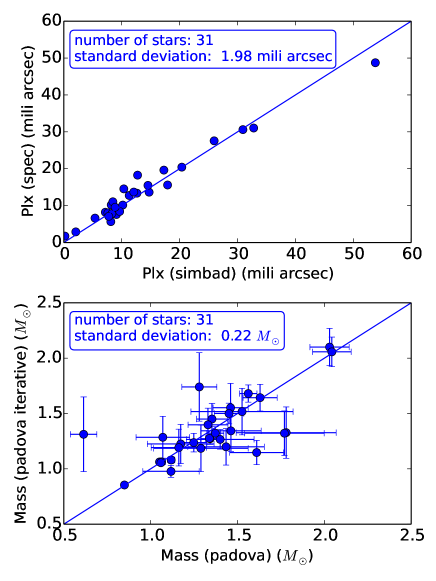
Figure 3: Top panel: Comparison between the parallax values found on SIMBAD and the derived spectroscopic parallax values. Bottom panel: Comparison between the estimated stellar mass using the different parallax values. These panels show that the iterative method to derive paralax/mass without the distance information works fairly well.

The presence of the outliers observed in Fig. 3 already alert us to be cautious with the use of fast stellar mass estimations like the tool that we are using here. For most of the cases we are able to derive masses within $\sim$ 10% accuracy, although there are some cases where the mass estimation has larger errors. We note that all five outlier stars in the bottom panel present larger errors than the rest of the stars. This issue should be considered very important, especially if we keep in mind that the inaccuracy on the stellar mass is transferred directly to the determination of the planetary masses ($M_{p}\propto M_{*}^{2/3}$, where $M_{p}$ and $M_{*}$ are the planetary and stellar masses, respectively). In Sect. 4.3 we discuss some examples where we bring up this issue again.

Table 12 contains the results that we obtained for the stellar mass, radius, age, as well as the visual magnitude and the parallax values used as input for the web interface tool. To keep consistency in the catalogue, for the few unevolved stars (with log g $\geq$ 4) we also derived the mass using the calibration of Torres et al. (2010). For this calibration we used the spectroscopic parameters derived previously and applied the small correction presented in Eq. (1) of Santos et al. (2013). These values are also presented in Table 12, and as expected, they are in good agreement with those derived with the web interface.

4.2 Comparison with literature

As in the previous section, we used the same online exoplanet databases to get values of masses and radius from the literature and compare them with our estimations. Figure 2 shows the result of the direct comparison of these fundamental parameters for the stars in common between our sample and each online database. For the cases where the errors for the mass or radius were not available in the online databases, we chose to adopt a 15% uncertainty, which is a conservative value when compared with the available values. The different comparisons of the masses are very similar for most of the stars, showing again that the online databases use the same sources for the majority of the stars in common. In the top panels we can see a significant large dispersion on the mass. There are five planet hosts that present significant offsets, but in this case all in the same direction. They are 14 And, HD 17092, HD 180314, HD 240237, and Omi CrB. We note that these stars are not the same outliers that appeared before when discussing the parallax values, except the case of HD 240237. For this star we note that using the iterative method we found a mass of 1.34 $M_{\sun}$, which is in between the values in Fig. 2 (0.61 $M_{\sun}$ and 1.69 $M_{\sun}$). In the next section we discuss in more detail the effect of our estimated mass values for these five outlier stars and the effect that it has on the respective planetary masses. Looking back at the top panels, if we neglect the three to five most extreme outlier stars present in each plot, we then obtain a better agreement between the masses that have less than half the original standard deviation ($\sim$ 0.2 $M_{\sun}$).

Because the stellar radius is also fundamental for the characterization of the transiting planet hosts, we present in the bottom panels of Fig. 2 the comparison of the stellar radius that we find in the same exoplanet databases. The results are generally in good agreement with only very few outliers. In the comparison with the values that we found in exo.eu the very strong outlier is again the star HD 240237. Looking again at the results obtained with the iterative method, we obtained a radius of 17.9 $R_{\sun}$ which is also in between the values in the plot (0.59 $R_{\sun}$ and 31 $R_{\sun}$). The three outliers present in the comparison with the radius for stars in common with exo.org are the planet hosts 11 UMi, 4 UMa, and HD 32518.

4.3 Impact of planetary masses

In this section we want to address the impact of the derived stellar mass on the planetary mass (here mass is defined as m$\sin i$ since most cases in this work are radial velocity detections, where $i$ is the orbital inclination to the line of sight). We exemplify this effect using the extreme outlier cases described in the previous section.

14 And:

Sato et al. (2008) have detected a giant planet with 4.8 $M_{jup}$ around 14 And, assuming a stellar mass of 2.2 $M_{\sun}$. Using our mass determination for this star, we can recalculate the planetary mass assuming the relation already mentioned ($M_{p}\propto M_{*}^{2/3}$). Using this relation and our mass determination (1.17 $M_{\sun}$) we reach a planetary mass of only 2.22 $M_{jup}$, which is a change of more than 100%. Recently, also for this planet host, Ligi et al. (2012) have reviewed the mass of this planet using interferometry. With a radius derived from interferometry of 12.82 $\pm$ 0.32 $R_{\sun}$, these authors then used the surface gravity derived in Sato et al. (2008) (2.63 dex) and the gravitational acceleration relation to derive a stellar mass reaching a value of 2.6 $\pm$ 0.42 $M_{\sun}$. If we do the same exercise using the stellar radius from interferometry together with our determination of surface gravity (2.44 dex) we reach a stellar mass of only 1.68 $M_{\sun}$, which then translates into a planetary mass of 3.18 $M_{jup}$, which still represents a difference of $\sim$ 66%.

HD 17092:

Niedzielski et al. (2007) reported the presence of a 4.6 $M_{jup}$ planet around HD 17092. A mass of 2.3 $M_{\sun}$ for the stellar host was adopted by these authors to derive the mass of the companion. Using our mass determination (1.25 $M_{\sun}$) we reach to a planetary mass of 2.2 $M_{jup}$. Again more than a 100% difference.

HD 180314:

This star represents another interesting case. Sato et al. (2010) detected a substellar companion around HD 180314 with 22 $M_{jup}$. The estimated stellar mass in this work was 2.6 $M_{\sun}$. If we use our stellar mass estimation of 2.04 $M_{\sun}$ we reach a less massive companion of 15.8 $M_{jup}$.

HD 240237:

This object was mentioned before because we found very different values for both its mass and radius. Doing the same exercise using the values reported in Gettel et al. (2012) (a 5.3 $M_{jup}$ giant planet derived with a stellar mass of 1.69 $M_{\sun}$) and using our mass determination of only 0.61 $M_{\sun}$ we obtain a planetary mass of only 1.53 $M_{jup}$.

omi CrB:

Sato et al. (2012) reported a 1.5 $M_{jup}$ giant planet orbiting around omi CrB, assuming a stellar mass of 2.13 $M_{\sun}$. With our mass determination of 1.07 $M_{\sun}$ we put the planet at a sub-Jupiter mass class with only 0.65 $M_{jup}$.

Our goal with these examples is not to state that our mass estimations are the best ones, defining therefore new, precise, and better planetary masses. Instead, we want to show that the estimation of the stellar mass for the planet hosts should be very well studied, especially in the more problematic case of evolved stars. On the one hand, it is known that the determination of spectroscopic stellar parameters can change significantly, in particular when using different line lists in the spectroscopic analysis (e.g., Taylor & Croxall, 2005; Santos et al., 2012; Mortier et al., 2013; Alves et al., 2015). On the other hand, the estimation of the fundamental parameters using stellar modeling can also lead to significant differences and interesting discussions such as the ones of Lloyd (2011, 2013) and Johnson et al. (2013). These simple examples presented here show that the different estimations of the stellar mass can change significantly the understanding of the discovered planets. Taking this to extreme examples, it can eventually reclassify the status of stellar companions.

4.4 Mass and metallicity in HD 139357

In the previous examples we showed that by using our mass estimation the planetary masses all changed to smaller values. We did not have any star that would produce the opposite scenario where the mass of the planet would be larger. Here we present such a case, but for this example the mass estimation is closely related with the metallicity of the star.

In Sect. 3.2. we report that the planet host HD 139357 has a large difference when comparing the metallicity derived in this work with the one that we found in the online databases. For the case of exo.eu, the values reported for metallicity and temperature are -0.13 dex and 4700 K, respectively, derived by Döllinger et al. (2009). If we use these values in the web-interface to estimate the stellar mass we obtain a value of 1.36 $\pm$ 0.18 $M_{\sun}$, which is in perfect agreement with the value used in the same work (1.35 $\pm$ 0.24 $M_{\sun}$) and which was used to derive a planetary mass of 9.76 $M_{jup}$.

If we go back to our parameters derived for this star, we have a temperature of 4595 K $\pm$ 76, which is compatible with the one derived by Döllinger et al. (2009). However, as reported in section 3.2. we obtained 0.19 dex for metallicity, corresponding to a large difference of 0.34 dex. The mass that we report in table 12 derived using our spectroscopic values is 1.78 $M_{\sun}$, which is significantly larger. Using this to recompute the planetary mass we obtain a value of 11.7 $M_{jup}$.

To test if this change could be due to the small difference in the derived effective temperature ($\sim$ 100 K) we used our spectroscopic parameters, changing only the metallicity, to derive the stellar mass again. The result is 1.33 $M_{\sun}$, which is very close to the value reported in Döllinger et al. (2009). This means that the stellar metallicity determination alone can be responsible for a change of 20% in the planetary mass for this extreme case. This example shows that we can also strongly underestimate a planetary mass in opposition with the examples that were described in the previous section.

5 Summary

We have collected high resolution and high signal-to-noise spectra with the NARVAL spectrograph. We used this data to derive new, precise, and homogeneous spectroscopic parameters using our standard analysis (ARES+MOOG) for 37 FGK planet host stars bright in different stages of evolution.

We also estimated the mass, radius, and age for all the stars in the sample following the same procedure as in previous works. The homogeneous parameters derived in this work were then included in the SWEET-Cat catalogue making it even more complete for the RV detected planets.

We compare our values with the ones available in online databases for exoplanets. The results are generally consistent, but we were able to identify some targets for which significant offsets are present, especially for the mass determination of a few giant stars in the sample.

We also discuss the effect of the stellar mass determination on the planetary mass. We show the most extreme cases for which the planetary masses may be overestimated. In addition, we also spotted an example with the opposite trend. In this case the source for the underestimation of the planetary mass is the stellar metallicity determination. We show with clear examples that it is fundamental to have precise stellar masses, which are not easy to obtain. To achieve this, spectroscopic stellar parameters are fundamental in order to constrain the stellar models.

Appendix A Spectroscopic parameters

Table 1: Spectroscopic parameters derived with ARES+MOOG.

Star ID	Teff	$\log{g}_{spec}$	$\xi_{\mathrm{t}}$	[Fe/H]	N(Fe i, Fe ii)	$\sigma$(Fe i, Fe ii)	Transiting planet
	[K]	[cm s-2]	[km s-1]	[dex]		[dex]	[Yes/No]
11 UMi	4255 $\pm$  88	1.80 $\pm$ 0.26	1.79 $\pm$ 0.08	-0.13 $\pm$ 0.04	113, 15	0.18, 0.30	No
14 And	4709 $\pm$  37	2.44 $\pm$ 0.12	1.51 $\pm$ 0.03	-0.29 $\pm$ 0.03	120, 15	0.09, 0.20	No
42 Dra	4452 $\pm$  42	2.09 $\pm$ 0.16	1.50 $\pm$ 0.04	-0.41 $\pm$ 0.03	117, 15	0.10, 0.29	No
4 Uma	4531 $\pm$  52	2.32 $\pm$ 0.14	1.54 $\pm$ 0.04	-0.19 $\pm$ 0.03	118, 15	0.11, 0.20	No
6 Lyn	5022 $\pm$  28	3.15 $\pm$ 0.13	1.16 $\pm$ 0.03	-0.10 $\pm$ 0.02	118, 14	0.06, 0.23	No
gam01 Leo	4395 $\pm$  48	1.66 $\pm$ 0.13	1.67 $\pm$ 0.04	-0.47 $\pm$ 0.03	118, 15	0.12, 0.21	No
HAT-P-14	6845 $\pm$ 108	4.62 $\pm$ 0.05	1.92 $\pm$ 0.15	0.17 $\pm$ 0.07	215, 34	0.19, 0.11	Yes
HAT-P-22	5351 $\pm$  57	4.22 $\pm$ 0.11	0.89 $\pm$ 0.10	0.28 $\pm$ 0.05	256, 33	0.13, 0.22	Yes
HD 100655	4891 $\pm$  46	2.79 $\pm$ 0.11	1.37 $\pm$ 0.04	0.07 $\pm$ 0.03	118, 15	0.10, 0.17	No
HD 102956	5010 $\pm$  37	3.31 $\pm$ 0.08	1.12 $\pm$ 0.04	0.12 $\pm$ 0.03	117, 15	0.08, 0.09	No
HD 116029	4819 $\pm$  54	2.98 $\pm$ 0.12	1.03 $\pm$ 0.06	0.09 $\pm$ 0.04	118, 15	0.11, 0.16	No
HD 118203	5890 $\pm$  41	4.10 $\pm$ 0.06	1.25 $\pm$ 0.04	0.30 $\pm$ 0.03	252, 33	0.10, 0.13	No
(1)	5910 $\pm$  35	4.18 $\pm$ 0.07	1.34 $\pm$ 0.04	0.25 $\pm$ 0.03	-	-	-
HD 131496	4886 $\pm$  45	3.16 $\pm$ 0.11	1.16 $\pm$ 0.05	0.12 $\pm$ 0.03	119, 15	0.09, 0.15	No
HD 132406	5766 $\pm$  23	4.19 $\pm$ 0.03	1.05 $\pm$ 0.03	0.14 $\pm$ 0.02	253, 35	0.06, 0.06	No
HD 132563B	6073 $\pm$  51	4.42 $\pm$ 0.05	1.02 $\pm$ 0.07	-0.06 $\pm$ 0.04	246, 35	0.11, 0.11	No
HD 136418	4979 $\pm$  44	3.43 $\pm$ 0.08	1.03 $\pm$ 0.05	-0.09 $\pm$ 0.03	118, 14	0.09, 0.08	No
HD 139357	4595 $\pm$  76	2.54 $\pm$ 0.20	1.61 $\pm$ 0.08	0.19 $\pm$ 0.05	117, 15	0.16, 0.31	No
HD 145457	4829 $\pm$  41	2.67 $\pm$ 0.10	1.48 $\pm$ 0.03	-0.13 $\pm$ 0.03	119, 15	0.09, 0.16	No
HD 152581	5095 $\pm$  23	3.31 $\pm$ 0.05	1.07 $\pm$ 0.02	-0.30 $\pm$ 0.02	119, 13	0.05, 0.07	No
HD 154345	5442 $\pm$  30	4.39 $\pm$ 0.04	0.76 $\pm$ 0.06	-0.13 $\pm$ 0.02	256, 33	0.07, 0.10	No
HD 158038	4822 $\pm$  64	3.06 $\pm$ 0.16	1.11 $\pm$ 0.07	0.16 $\pm$ 0.05	119, 15	0.13, 0.23	No
HD 16175	6022 $\pm$  34	4.21 $\pm$ 0.06	1.26 $\pm$ 0.03	0.37 $\pm$ 0.03	255, 35	0.08, 0.13	No
(1)	6030 $\pm$  22	4.23 $\pm$ 0.04	1.39 $\pm$ 0.02	0.32 $\pm$ 0.02	-	-	-
HD 163607	5586 $\pm$  29	4.05 $\pm$ 0.05	1.09 $\pm$ 0.03	0.22 $\pm$ 0.02	255, 35	0.07, 0.12	No
HD 17092	4596 $\pm$  65	2.45 $\pm$ 0.17	1.55 $\pm$ 0.06	0.05 $\pm$ 0.04	118, 15	0.14, 0.25	No
HD 173416	4783 $\pm$  43	2.43 $\pm$ 0.09	1.49 $\pm$ 0.03	-0.15 $\pm$ 0.03	118, 14	0.10, 0.10	No
HD 180314	4913 $\pm$  60	2.90 $\pm$ 0.17	1.45 $\pm$ 0.05	0.11 $\pm$ 0.04	119, 15	0.13, 0.28	No
HD 197037	6150 $\pm$  34	4.37 $\pm$ 0.04	1.11 $\pm$ 0.04	-0.16 $\pm$ 0.03	235, 36	0.08, 0.09	No
HD 219415	4787 $\pm$  53	3.22 $\pm$ 0.11	1.00 $\pm$ 0.06	0.03 $\pm$ 0.03	118, 14	0.10, 0.10	No
HD 222155	5750 $\pm$  23	4.00 $\pm$ 0.05	1.13 $\pm$ 0.02	-0.09 $\pm$ 0.02	253, 34	0.06, 0.11	No
(2)	5765 $\pm$  22	4.10 $\pm$ 0.13	1.22 $\pm$ 0.02	-0.11 $\pm$ 0.05	-	-	-
HD 240210	4316 $\pm$  78	1.91 $\pm$ 0.21	1.76 $\pm$ 0.07	-0.14 $\pm$ 0.03	115, 15	0.16, 0.26	No
HD 240237	4422 $\pm$ 101	1.69 $\pm$ 0.24	2.31 $\pm$ 0.08	-0.24 $\pm$ 0.06	111, 14	0.19, 0.30	No
HD 32518	4661 $\pm$  53	2.41 $\pm$ 0.12	1.53 $\pm$ 0.05	-0.10 $\pm$ 0.04	119, 13	0.12, 0.16	No
HD 96127	4179 $\pm$ 110	1.59 $\pm$ 0.34	2.01 $\pm$ 0.11	-0.29 $\pm$ 0.05	114, 14	0.23, 0.40	No
HD 99706	4891 $\pm$  35	3.07 $\pm$ 0.08	1.15 $\pm$ 0.03	0.02 $\pm$ 0.03	119, 15	0.07, 0.12	No
kappa CrB	4889 $\pm$  48	3.20 $\pm$ 0.11	1.13 $\pm$ 0.04	0.11 $\pm$ 0.03	120, 15	0.09, 0.14	No
Kepler-21	6269 $\pm$  47	4.07 $\pm$ 0.06	1.35 $\pm$ 0.05	0.03 $\pm$ 0.03	236, 34	0.10, 0.12	Yes
omi CrB	4792 $\pm$  35	2.65 $\pm$ 0.14	1.48 $\pm$ 0.03	-0.23 $\pm$ 0.03	119, 15	0.07, 0.25	No

Appendix B Stellar masses and radii

Table 2: Estimations of the stellar masses, radii, and ages for the planet hosts.

Star ID	V mag	Plx	Mass (Padova)	Mass (Torres)	Radius (Padova)	Age (Padova)
		mili arcsec	$M_{\sun}$	$M_{\sun}$	$R_{\sun}$	Gyr
11UMi	5.02	8.19  $\pm$  0.19	1.434 $\pm$ 0.220	-	27.032  $\pm$ 2.135	3.186 $\pm$ 1.521
14And	5.22	12.63  $\pm$  0.27	1.173 $\pm$ 0.192	-	10.859  $\pm$ 0.409	5.477 $\pm$ 3.089
42Dra	4.83	10.36  $\pm$  0.20	1.117 $\pm$ 0.162	-	19.507  $\pm$ 0.655	5.911 $\pm$ 3.002
4Uma	4.60	12.74  $\pm$  0.26	1.610 $\pm$ 0.155	-	16.751  $\pm$ 0.704	2.080 $\pm$ 0.625
6Lyn	5.88	17.92  $\pm$  0.47	1.562 $\pm$ 0.050	-	4.830  $\pm$ 0.164	2.353 $\pm$ 0.211
gam01Leo	2.12	25.96  $\pm$  0.83	1.462 $\pm$ 0.174	-	28.395  $\pm$ 1.458	2.412 $\pm$ 0.879
HAT-P-14	9.99	6.42*	1.427 $\pm$ 0.048	1.364	1.426  $\pm$ 0.078	0.431 $\pm$ 0.295
HAT-P-22	9.76	9.87*	0.959 $\pm$ 0.024	0.985	1.084  $\pm$ 0.120	9.407 $\pm$ 3.130
HD100655	6.44	8.18  $\pm$  0.50	2.030 $\pm$ 0.113	-	8.891  $\pm$ 0.483	1.309 $\pm$ 0.236
HD102956	7.85	7.92  $\pm$  0.83	1.630 $\pm$ 0.098	-	4.275  $\pm$ 0.453	2.328 $\pm$ 0.418
HD116029	7.89	8.12  $\pm$  0.65	1.280 $\pm$ 0.101	-	4.693  $\pm$ 0.406	4.855 $\pm$ 1.307
HD118203	8.06	11.29  $\pm$  0.70	1.342 $\pm$ 0.055	1.279	1.829  $\pm$ 0.119	3.578 $\pm$ 0.492
HD131496	7.80	9.09  $\pm$  0.78	1.353 $\pm$ 0.089	-	4.132  $\pm$ 0.368	4.060 $\pm$ 0.821
HD132406	8.45	14.73  $\pm$  0.61	1.051 $\pm$ 0.014	1.105	1.245  $\pm$ 0.055	7.187 $\pm$ 0.660
HD132563B	9.61	9.12*	1.081 $\pm$ 0.029	1.049	1.092  $\pm$ 0.080	2.310 $\pm$ 1.886
HD136418	7.88	10.18  $\pm$  0.58	1.248 $\pm$ 0.076	1.303	3.463  $\pm$ 0.220	4.649 $\pm$ 0.985
HD139357	5.98	8.47  $\pm$  0.30	1.780 $\pm$ 0.288	-	12.394  $\pm$ 0.941	2.028 $\pm$ 0.937
HD145457	6.57	7.98  $\pm$  0.45	1.526 $\pm$ 0.294	-	9.483  $\pm$ 0.907	2.605 $\pm$ 1.608
HD152581	8.35	5.39  $\pm$  0.96	1.400 $\pm$ 0.195	-	4.370  $\pm$ 1.177	2.850 $\pm$ 1.112
HD154345	6.74	53.80  $\pm$  0.32	0.849 $\pm$ 0.015	0.862	0.869  $\pm$ 0.008	9.527 $\pm$ 1.662
HD158038	7.46	9.65  $\pm$  0.74	1.330 $\pm$ 0.115	-	4.858  $\pm$ 0.418	4.433 $\pm$ 1.223
HD16175	7.28	17.28  $\pm$  0.67	1.338 $\pm$ 0.022	1.292	1.633  $\pm$ 0.070	2.802 $\pm$ 0.162
HD163607	7.98	14.53  $\pm$  0.46	1.118 $\pm$ 0.021	1.146	1.695  $\pm$ 0.063	7.581 $\pm$ 0.475
HD17092	7.73	4.59*	1.246 $\pm$ 0.179	-	10.439  $\pm$ 1.310	5.580 $\pm$ 2.669
HD173416	6.06	7.17  $\pm$  0.28	1.770 $\pm$ 0.229	-	12.422  $\pm$ 0.674	1.730 $\pm$ 0.653
HD180314	6.61	7.61  $\pm$  0.39	2.043 $\pm$ 0.111	-	8.911  $\pm$ 0.434	1.295 $\pm$ 0.234
HD197037	6.81	30.93  $\pm$  0.38	1.063 $\pm$ 0.022	1.059	1.105  $\pm$ 0.023	3.408 $\pm$ 0.924
HD219415	8.91	5.89*	1.138 $\pm$ 0.100	-	4.098  $\pm$ 0.640	7.233 $\pm$ 2.295
HD222155	7.12	20.38  $\pm$  0.62	1.059 $\pm$ 0.018	1.135	1.685  $\pm$ 0.059	7.854 $\pm$ 0.407
HD240210	8.27	2.41*	1.241 $\pm$ 0.238	-	19.293  $\pm$ 4.399	5.085 $\pm$ 3.089
HD240237	8.17	0.19  $\pm$  0.72	0.614 $\pm$ 0.076	-	0.587  $\pm$ 0.274	4.420 $\pm$ 4.007
HD32518	6.42	8.29  $\pm$  0.58	1.162 $\pm$ 0.159	-	10.499  $\pm$ 0.567	6.468 $\pm$ 3.058
HD96127	7.41	2.07  $\pm$  0.58	1.289 $\pm$ 0.272	-	31.610  $\pm$ 7.414	4.067 $\pm$ 2.624
HD99706	7.64	7.76  $\pm$  0.68	1.460 $\pm$ 0.101	-	5.120  $\pm$ 0.465	3.085 $\pm$ 0.625
kappaCrB	4.80	32.79  $\pm$  0.21	1.451 $\pm$ 0.085	-	4.791  $\pm$ 0.165	3.286 $\pm$ 0.554
Kepler-21	8.25	8.86  $\pm$  0.58	1.372 $\pm$ 0.049	1.359	1.863  $\pm$ 0.126	2.818 $\pm$ 0.341
omiCrB	5.52	12.08  $\pm$  0.44	1.070 $\pm$ 0.154	-	10.216  $\pm$ 0.351	7.827 $\pm$ 3.844