Anharmonicity changes the solid solubility of a random alloy at high temperatures — supplementary information

I Methodological details

In order to find the effective force constant matrix that best represents the Born-Oppenheimer potential energy surface, we minimize the difference in forces between the model system and the SQS model of a real alloy, computing the latter by means of ab initio molecular dynamics (AIMD). We seek the linear least squares solution for the force constants $\mathbf{\bar{\bar{\Phi}}}^{\textrm{eff}}_{ij}$ that minimize the difference in forces $\Delta\mathbf{F}$ between AIMD and our Hamiltonian form $\{\mathbf{F}_{t}^{\textrm{m}}\}$.

$$\begin{split}\min_{\mathbf{\bar{\bar{\Phi}}}}\Delta\mathbf{F}&=\frac{1}{N_{t}}\sum_{t=1}^{N_{t}}\left|\mathbf{F}_{t}^{\textrm{MD}}-\mathbf{F}_{t}^{\textrm{H}}\right|^{2}\\ &=\frac{1}{N_{t}}\sum_{t=1}^{N_{t}}\left|\mathbf{F}_{t}^{\textrm{MD}}-\mathbf{\bar{\bar{\Phi}}}^{\textrm{eff}}\mathbf{U}_{t}^{\textrm{MD}}\right|^{2},\end{split}$$ (1)

where $\{\mathbf{U}_{t}^{\textrm{MD}}\}$ and $\{\mathbf{F}_{t}^{\textrm{MD}}\}$ are sets of displacements and forces from AIMD respectively.

TDEP potential energy surface is given by

$$U_{\textrm{TDEP}}(t)=U_{0}(t)+\frac{1}{2}\sum_{ij}\mathbf{u}_{i}(t)\mathbf{\bar{\bar{\Phi}}}^{\textrm{eff}}_{ij}(t)\mathbf{u}_{j}(t),$$ (2)

where $\mathbf{u}_{i,j}$ are displacement of atoms i, j respectively and $t$ is time. $U_{0}$ is a non-harmonic term, containing the renomalized baseline for the TDEP quasiparticles. It is determined from the criteria that the average potential energy from MD and TDEP should be equal:

$$U_{0}(T)=\left\langle U_{\textrm{MD}}(t)-\frac{1}{2}\sum_{ij}\mathbf{u}_{i}(t)\mathbf{\bar{\bar{\Phi}}}^{\textrm{eff}}_{ij}(t)\mathbf{u}_{j}(t)\right\rangle,$$ (3)

where the brackets indicate a configuration (time) average at temperature $T$. To extract only the non-harmonic renormalization term we take the difference between between 0 K energies and calculated $U_{0}$ in eq. (3):

$$\Delta U_{0}(T)=U_{0}(T)-U_{el}.$$ (4)

This term later is added to the vibrational free energy in eq. (3) in the main text.

II Computational details

II.1 Ab initio molecular dynamics

Canonical ensemble ab initio molecular dynamics simulations were performed using the projector-augmented wave (PAW) method Blöchl (1994) as implemented in VASPKresse and Hafner (1993); Kresse and Furthmüller (1996a, b); Kresse (1999) over a range of temperatures, volumes, and concentrations. The temperature was set with a Nosé thermostat Nosé (1984); Hoover (1985) with Fermi smearing corresponding to the simulation temperature. The plane wave energy cutoff was set to 600 eV and the Brillouin zone (BZ) was sampled at the Gamma point. The random alloy was generated using a special quasirandom structure (SQS) approach Zunger et al. (1990). A 128 atom SQS ($4\times 4\times 4$) supercell was constructed, in which 64 atoms were metal and 64 were nitrogen. Three different SQS were generated, corresponding to different compositions of the random Ti_1-xAl_xN alloy, with B1 symmetry and $x$=$\{$0.25,0.5,0.75$\}$. 128 atoms SQS was generated trying to mimic the SRO parameters of perfect random alloys for the first 7 coordination shells for pair interactions with extra focus on the first 5. The small-radius 4 and 3-site clusters where taken into account, but focus was on pairs. For Al-rich compositions all configurational interactions become strong, but the short range 2-site interactions give the largest contribution to the energy. We assume that the vibrational free energy shows a qualitatively similar dependence with respect to energy on 2-site correlation functions as it does with 3- and 4-site functions.

A subset of uncorrelated samples from the AIMD simulations was selected and upsampled to high accuracy with a $3\times 3\times 3$ k-point mesh for the BZ integration. The effective force constants where found to be smooth and easily interpolated across the whole concentration interval, giving the phonon DOS as a continuous function of concentration, volume and temperature.

II.2 Thermodynamic integration

Thermodynamic integration was used to validate our choice of Hamiltonian. A Langevin thermostat was used to control the temperature and break the mode-locking. The numerical integration over coupling parameter $\lambda$ was carried out over 5 discrete steps, and the MD simulations were run for $\sim$100 000 timesteps with k-point sampling at the Gamma-point only. A set of uncorrelated snapshots was selected from AIMD and upsampled to high accuracy with a $3\times 3\times 3$ k-point mesh to ensure convergence for $\Delta F$.

II.3 Benchmark test

We perform a series of additional calculations to check the reliability of our method. Using the small displacement method, the harmonic vibrational Gibbs free energy was calculated for the full SQS, treating all atoms as non-equivalent and thus including local environment effects in the force constants. This was compared to the SIFC-TDEP vibrational Gibbs free energy (Fig. 1 in the main text). Harmonic phonon free energies are compared at a specific concentration (Ti_0.5Al_0.5N) and volume/atom (9.1260 ų). For the small displacement method, force constants are taken at zero temperature, while “SIFC-TDEP” denotes a free energy calculated using SIFC-TDEP force constants. At high temperature, the harmonic approximation is no longer a good benchmark, even at constant volume. In this case, we benchmarked using UP-TILD, which is formally exact in that region. Fig. 1 shows the comparison of the phonon free energies at the same volume taken at 1500 K. The free energy calculated using temperature-dependent force constants and the anharmonic correction ($\Delta U_{0}$) lies closer to the thermodynamic integration point. Omitting anharmonic effects leads to the underestimation of the phonon contribution (Fig. 1).

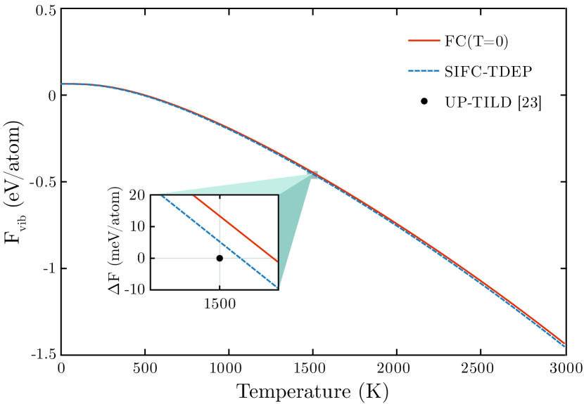
Figure 1: (Color online) Phonon free energy as a function of temperature at constant volume. Harmonic free energy calculated with force constants extracted at 0K using small displacement method (red solid line). Harmonic free energy calculated using SIFC-TDEP with the force constants and $\Delta U_{0}$ at the same volume (1500 K) is shown by blue dashed line. Free energy calculated by upsampled thermodynamic integration using Langevin dynamics is shown as the black point. We include the insert showing the difference between mentioned above free energies at 1500 K taking the thermodynamic integration point as a reference.

III Phase diagram reconstruction

G${}_{mix}(\mathbf{x})$ is defined as a function of the vector $\mathbf{x}$ in composition space. In the general case at a given pressure and temperature, a mixture of $N_{c}$ atomic species, or components, may split into $N_{p}$ distinct phases. We define a $N_{c}\times N_{p}-1$ grid of compositions $\mathbf{x}$ with elements $x_{ik}$, where element $x_{ik}$ is an atomic fraction of component $i$ in phase $k$. The solution must satisfy two constraints Gibbs (1871) : the component material balance constraint and the positive value of the atomic fraction of components in the system:

$$\sum_{i=1}^{N_{c}}\sum_{k=1}^{N_{p}-1}x_{ik}=1,$$ (5)

$$0\leq x_{ik}\leq x_{i}.$$

The Gibbs free energy can be expressed as discrete function

$$G(\mathbf{x})=\sum\limits_{i=1}^{N_{c}}\sum\limits_{k=1}^{N_{p}-1}x_{ik}G_{ik}.$$ (6)

The mass balance constraint can be rewritten in matrix form $\mathbf{A}\mathbf{x}=\mathbf{B}$, or

$$\sum\limits_{i=1}^{N_{c}}\sum\limits_{k=1}^{N_{p}-1}a_{ei}x_{ik}=B,$$ (7)

where $e$ is an index of number of possible combinations of fractions of component $i$ and a_ei are the matrix elements. B is a global concentration of component $i$ in the initial solid solution phase.

We consider the Gibbs free energy of mixing. There are two phases or distinct regions (k=2); one is a solid solution of Ti_1-xAl_xN and the other is the miscibility region.

$$G_{mix}(\mathbf{x})=\sum\limits_{i=1}^{N_{c}}G^{mix}_{i}.$$ (8)

To recover the phase diagram, we minimise $G_{\mathrm{mix}}$ or $G$ subject to the constraint (7).

This can be done via, for example, the method of constrained least squares Antoniou and Lu (2007). In order to construct the phase diagram, we repeat this procedure over a range of temperatures in the regime of interest.

This is a convenient methodology since no assumptions about reactions are necessary, and the constraints are easy to identify. There is also no need to define $G$ across the entire concentration interval if we have a many phase system, which removes complications such as the presence of dynamically unstable phases. Furthermore the proposed technique removes the need to numerically calculate derivatives of the Gibbs free energy needed in state-of-the-art methods for constructing phase diagrams, a procedure that is notoriously sensitive to numerical noise. Of course in our case, we still determine the spinodal from the condition ($\frac{\partial^{2}G_{mix}}{\partial x^{2}}|_{T}\leq 0$).

IV Experimental details

Atom probe tomography (APT) samples were prepared in a dual-beam focused ion beam/scanning electron microscopy workstation (FIB/SEM) (Helios NanoLab 600${}^{\textrm{TM}}$, FEI Company, USA) by the standard lift-out technique Thompson et al. (2007). Laser Pulsed APT was carried out with a LEAP${}^{\textrm{TM}}$ 3000X HR (CAMECA) at a repetition rate of 200 kHz, a specimen temperature of about 60 K, a pressure lower than 1 $\times$ 10^-10 Torr (1.33 $\times$ 10^-8 Pa), and a laser pulse energy of 0.5 nJ. The evaporation rate of the specimen was 5 atoms per 1000 pulses. The positions and the time-of-flight of the ions coming into the detector are used to generate a three-dimensional reconstruction with IVAS${}^{\textrm{TM}}$3.6.6 software (CAMECA). The accuracy of atomic-scale of APT and concentration are discussed in literature Seidman (2007); Allen et al. (2008); Kim et al. (2014); Biswas et al. (2014). Previous results demonstrate that it is now possible to obtain highly quantitative information from APT.

References

- Blöchl (1994) P. E. Blöchl, Physical Review B 50, 17953 (1994).
- Kresse and Hafner (1993) G. Kresse and J. Hafner, Physical Review B 48, 13115 (1993).
- Kresse and Furthmüller (1996a) G. Kresse and J. Furthmüller, Physical Review B 54, 11169 (1996a).
- Kresse and Furthmüller (1996b) G. Kresse and J. Furthmüller, Computational Materials Science 6, 15 (1996b).
- Kresse (1999) G. Kresse, Physical Review B 59, 1758 (1999).
- Nosé (1984) S. Nosé, Molecular Physics 52, 255 (1984).
- Hoover (1985) W. Hoover, Physical Review A 31, 1695 (1985).
- Zunger et al. (1990) A. Zunger, S. H. Wei, L. G. Ferreira, and J. Bernard, Physical Review Letters 65, 353 (1990).
- Gibbs (1871) J. W. Gibbs, A Method of Geometrical Representation of the Thermodynamic Properties of Substances by Means of Surfaces, Vol. Volumes 38 (The Academy, 1871).
- Antoniou and Lu (2007) A. Antoniou and W. S. Lu, Practical Optimization: Algorithms and Engineering Applications (Springer, 2007).
- Thompson et al. (2007) K. Thompson, D. Lawrence, D. J. Larson, J. D. Olson, T. F. Kelly, and B. Gorman, Ultramicroscopy 107, 131 (2007).
- Seidman (2007) D. N. Seidman, Annual Review of Materials Research 37, 127 (2007).
- Allen et al. (2008) J. E. Allen, E. R. Hemesath, D. E. Perea, J. L. Lensch-Falk, Z. Y. Li, F. Yin, M. H. Gass, P. Wang, A. L. Bleloch, R. E. Palmer, and L. J. Lauhon, Nature nanotechnology 3, 168 (2008).
- Kim et al. (2014) Y.-J. Kim, J. D. Weiss, E. E. Hellstrom, D. C. Larbalestier, and D. N. Seidman, Applied Physics Letters 105, 162604 (2014).
- Biswas et al. (2014) A. Biswas, D. J. Siegel, and D. N. Seidman, Acta Materialia 75, 322 (2014).