Exchange interaction between $J$-multiplets

Abstract

Analytical expressions for the exchange interaction between $J$-multiplets of interacting metallic centers are derived on the basis of a complete electronic model which includes the intrasite relativistic effects. A common belief that this interaction can be approximated by an isotropic form $\propto{\mathbf{J}}_{1}\cdot{\mathbf{J}}_{2}$ (or $\propto{\mathbf{J}}_{1}\cdot{\mathbf{S}}_{2}$ in the case of interaction with an isotropic spin) is found to be ungrounded. It is also shown that the often used “$1/U$ approximation” for the description of the kinetic contribution of the exchange interaction is not valid in the case of $J$-multiplets. The developed theory can be used for microscopic description of exchange interaction in materials containing lanthanides, actinides and some transition metal ions.

I Introduction

Strong magnetic anisotropy induced by spin-orbit coupling on the metal sites is a key ingredient for a number of intriguing properties of magnetic materials, such as single-molecule magnet behavior Gatteschi et al. (2006); Layfield and Murugesu (2015), magnetic multipole ordering Santini et al. (2009), and various exotic electronic phases Witczak-Krempa et al. (2014); Gingras and McClarty (2014). If the spin-orbit coupling exceeds the crystal-field splitting of the ground term $LS$ on the metal site, the latter acquires unquenched orbital momentum $\hat{\mathbf{L}}$ and the low-lying spectrum is well described as crystal-field split eigenstates of the total angular momentum $\hat{\mathbf{J}}=\hat{\mathbf{L}}+\hat{\mathbf{S}}$, where $\hat{\mathbf{S}}$ is the spin of the metallic term. This situation takes place in lanthanides Wybourne (1965), actinides Santini et al. (2009) and some transition metal ions in a cubic symmetry environment Griffith (1971); Abragam and Bleaney (1970).

The exchange interaction between such split-$J$ crystal-field levels (or groups of levels) is significantly more complicated than the exchange interaction between pure spin terms ($L=0$) described by the Heisenberg Hamiltonian $\mathcal{J}\hat{\mathbf{S}}_{1}\cdot\hat{\mathbf{S}}_{2}$. For the weak spin-orbit coupling, the discrepancy of the exchange Hamiltonian from the isotropic form was first pointed out by Stevens Stevens (1953). Later, the anisotropic exchange interaction was extensively developed by Moriya Moriya (1960) based on the Anderson’s microscopic approach Anderson (1959, 1963). In the case of the strong spin-orbit coupling, the exchange interaction including the higher order terms of $\hat{\mathbf{J}}$ was also phenomenologically treated since long time ago Levy (1964); Birgeneau et al. (1969). The microscopic description was addressed for the first time by Elliott and Thorpe Elliott and Thorpe (1968) for uranium oxides, and by Hartmann-Boutron Hartmann-Boutron (1968) for transition metal compounds on the basis of simplified analysis based on so-called $1/\bar{U}$ approximation ($\bar{U}$ is the average electron promotion energy between the sites). Recently, within the same approximation, the microscopic derivation of the exchange Hamiltonian between $J$-multiplets was completed by Santini et al. Santini et al. (2009).

Despite this early evidence of complexity of exchange interaction between metal ions with unquenched orbital moments, it was repeatedly conjectured that the exchange interaction between fully degenerate $J$-shells, involving $(2J_{1}+1)$ and $(2J_{2}+1)$ angular momentum eigenstates on the first and the second magnetic centers, respectively, is described by an isotropic exchange Hamiltonian written in terms of $\hat{\mathbf{J}}_{i}$ momenta:

$$\hat{H}_{\text{Heis}} = \mathcal{J}\hat{\mathbf{J}}_{1}\cdot\hat{\mathbf{J}}_{2}.$$ (1)

Contrary to Heisenberg Hamiltonian for isotropic spins, there is no a priori justification for the Hamiltonian (1). Nevertheless, this form is often used for the description of interaction between lanthanides or actinides (or a similar form, $\propto\hat{\mathbf{J}}_{1}\cdot\hat{\mathbf{S}}_{2}$, in the case of their interaction with an isotropic spin), especially, in the last years Molavian et al. (2007); Talbayev et al. (2008); Curnoe (2008); Arnold et al. (2010); Magnani et al. (2010); Lukens et al. (2012); Carretta et al. (2013); Przychodzen et al. (2007); Yamaguchi et al. (2008); Klokishner et al. (2009); Klokishner and Reu (2012); Reu et al. (2013); Dreiser et al. (2012); Kofu et al. (2013). One of the reasons that the simple bilinear form has been often used is that the large numbers of the phenomenological exchange parameters cannot be easily determined.

It is not clear, however, how important are “non-Heisenberg” terms in the actual $J$-$J$ coupling, nor is the $1/\bar{U}$ approximation a priori justified for metal ions with unquenched orbital momenta. Both these questions can only be answered after a more complete derivation of exchange interaction between $J$ multiplets on the basis of a reliable microscopic model. Besides, a microscopic description of $J$-$J$ ($J$-$S$) exchange interaction is desirable due to a very large number of phenomenological parameters, in contrast to weakly-anisotropic spin systems containing only a few of them Bencini and Gatteschi (1990); Chibotaru (2015). Given that many microscopic electronic parameters describing individual magnetic centers and their interaction can be accurately derived via density functional theory Imada and Miyake (2010) or ab initio calculations Ungur and Chibotaru (2015), a microscopically derived Hamiltonian for $J$ multiplets can become a powerful tool for the investigation of exchange interaction in materials containing lanthanides, actinides and transition metal ions with unquenched orbital momentum. To this end the electronic Hamiltonians only need to be downfolded on the reduced manifold of low-lying states at the corresponding metal ions.

In this work, we derive analytically the exchange Hamiltonians for interacting $J$-multiplets and for interacting $J$-multiplet and isotropic spin, starting from a microscopic electronic Hamiltonian including the relativistic interactions on the metal sites. The obtained exchange parameters are expressed via electronic matrix elements which can be derived from electronic structure calculations. The structure of the exchange Hamiltonian is discussed and the result is applied for the analysis of some systems with different geometries. Comparison with the predictions given by the Hamiltonian (1) and the simplified treatment on the basis of $1/\bar{U}$ approximation shows that both of them are not suitable approaches to describe the exchange interaction of ions with unquenched orbital momentum. Finally, the relative contributions to the kinetic exchange interaction from intermediate states is analyzed.

II Microscopic description of intersite interaction

We derive the expression for the interaction between metal ions with unquenched orbital moments. The derivation is based on a complete electronic Hamiltonian, including all intrasite relativistic effects, and employs adequate approximations. The multipolar intersite interactions of electromagnetic type, such as the electric quadrupolar and magnetic dipolar interactions, have been described elsewhere Santini et al. (2009); Birgeneau et al. (1969); Birgeneau (1967); Zvezdin et al. (1985) and are not considered here. Their effect can be taken into account as additive contribution to the exchange parameters.

II.1 Electronic multiplets on sites

The nonrelativistic electronic state of an ion with partially filled $nl$ shell ($n$ is the main quantum number and $l$ is the one-electron orbital angular momentum) corresponds to an $LS$-term characterized by the total orbital $\hat{\mathbf{L}}$ and spin $\hat{\mathbf{S}}$ angular momenta Landau and Lifshitz (1977). The eigenfunctions $\{|\alpha_{LS}LM_{L}SM_{S}\rangle\}$ are described by orbital and spin quantum numbers, $L$ and $S$, and the projections of $\hat{\mathbf{L}}$ and $\hat{\mathbf{S}}$ on a given axis $z$, $M_{L}$ and $M_{S}$, respectively; $\alpha_{LS}$ indicates the other quantum numbers. The $(2L+1)(2S+1)$-fold degenerate term is further split by the spin-orbit interaction into $J$-multiplets which are eigenstates of the total angular momentum $\hat{\mathbf{J}}=\hat{\mathbf{L}}+\hat{\mathbf{S}}$. The corresponding eigenfunctions $\{|\alpha_{J}JM\rangle\}$ are characterized by quantum numbers of the total angular momentum $J$ and its projection $M=-J,-J+1,\cdots J$ ($\alpha_{J}$ stands for other quantum numbers).

In general, the spin-orbit interaction mixes multiplets with the same $J$ belonging to different $LS$ terms (the so-called $J$-$J$ mixing Zvezdin et al. (1985)). In the case when this mixing can be neglected, each $J$-multiplet is attributed to one $LS$-term and the corresponding wave functions become of the form ($\alpha_{J}=(\alpha_{LS},L,S)$):

$$|\alpha_{J}JM\rangle = \sum_{M_{L}M_{S}}|\alpha_{LS}LM_{L}SM_{S}\rangle C_{LM_{L}SM_{L}}^{JM},$$ (2)

where $C_{LM_{L}SM_{L}}^{JM}$ is the Clebsch-Gordan coefficient (49) Varshalovich et al. (1988). This is a good approximation, in particular, for the ground $J$-multiplet of trivalent ions from the late lanthanides series, Ln³⁺.

When the metal ions are embedded in complexes or crystals, their electronic structure is modified due to covalent and electrostatic interaction of the magnetic $nl$ orbitals with the environment. In the case of $f$-metals the magnetic orbitals are usually strongly localized and the effect of the surrounding is relatively weak. For example, in the case of lanthanide, the intraionic bielectronic interaction leading to atomic terms separation is ca 5-7 eV and the spin-orbit splitting is ca 1 eV for lanthanide ions, thus exceeding several times the the crystal-field splitting, which is usually of the order of 0.1 eV van der Marel and Sawatzky (1988). In this situation the low-energy electronic states are well approximated as crystal-field split atomic $J$-multiplets. Due to the weak hybridization of the $4f$ orbitals with the surrounding, the Wannier functions of the corresponding magnetic orbitals practically coincide with the atomic $4f$ orbitals. Similar holds true for actinide ions although $5f$ orbitals are more delocalized than $4f$ orbitals.

On the other hand, the effect of the hybridization of $d$ orbitals with the ligand orbitals is usually much stronger than in lanthanides and actinides resulting in a crystal-field splitting which often overcomes the atomic $LS$-term splitting. Therefore, the orbital angular momentum is generally not a good quantum number for nondegenerate ground state of embedded transition metal ions. Moreover this orbital angular momentum is quenched as a rule, $\langle\hat{\mathbf{L}}\rangle=0$, in most compounds. The exception is the cubic environment, in which the $d$ orbitals split into doubly degenerate $e$ and triply degenerate $t_{2}$ levels. When the $t_{2}$ orbital are partially filled, the electronic state is characterized by the nonzero fictitious orbital angular momentum $\tilde{L}=1$, which couples to the total spin of the site via spin-orbit coupling and gives molecular multiplets characterized by fictitious total angular momentum $\tilde{\mathbf{J}}=\tilde{\mathbf{L}}+\hat{\mathbf{S}}$ (see Ref. Abragam and Bleaney, 1970 for details).

II.2 Intersite interaction

The electronic Hamiltonian $\hat{H}$ for electrons localized at two sites can be divided into the intrasite contributions $\hat{H}_{0}^{i}$ $(i=1,2)$, the intersite bielectronic $\hat{H}_{\text{bi}}^{\prime}$ and electron transfer $\hat{H}_{\text{t}}$ parts:

$$\hat{H} = \sum_{i=1,2}\hat{H}_{0}^{i}+\hat{H}^{\prime}_{\text{bi}}+\hat{H}_{\text{t}}.$$ (3)

The intrasite Hamiltonian for site $i$, $\hat{H}_{0}^{i}$, contains all effects discussed in Sec. II.1 such as the non-relativistic atomic terms, the spin-orbit term and other relativistic corrections, and the crystal-field. The eigenstate of $\hat{H}_{0}^{i}$ is determined by the number of electrons $N_{i}$ in magnetic orbitals and crystal-field level $p$, $|iN_{i},p\rangle$. $\hat{H}_{\rm bi}^{\prime}$ consists of intersite Coulomb interaction $\hat{H}_{\rm Coul}$ and direct exchange (multipole) part $\hat{H}_{\rm DE}$:

$$\hat{H}^{\prime}_{\rm bi} = \hat{H}_{\rm Coul}+\hat{H}_{\rm DE},$$ (4)

$$\hat{H}_{\rm Coul} = \sum_{mn\sigma\sigma^{\prime}}U^{\prime}\hat{n}_{1m\sigma}\hat{n}_{2n\sigma^{\prime}},$$ (5)

$$\hat{H}_{\rm DE} = -\sum_{mnm^{\prime}n^{\prime}\sigma\sigma^{\prime}}V_{mm^{\prime}n^{\prime}n}\hat{c}_{1m\sigma}^{\dagger}\hat{c}_{1n\sigma^{\prime}}\hat{c}_{2m^{\prime}\sigma^{\prime}}^{\dagger}\hat{c}_{2n^{\prime}\sigma},$$ (6)

where $m,n$ indicate the projection of the orbital angular momentum $l_{i}$, $\sigma$ is the projection of the electron spin momentum, $\hat{c}_{im\sigma}^{\dagger}$ ($\hat{c}_{im\sigma}$) is the electron creation (annihilation) operator in spin-orbital $(m,\sigma)$ of site $i$ $(=1,2)$, $\hat{n}_{im\sigma}=\hat{c}^{\dagger}_{im\sigma}\hat{c}_{im\sigma}$, $U^{\prime}$ is the intersite electron repulsion, $V_{mm^{\prime}n^{\prime}n}$ is the intersite exchange integral,

$$V_{mm^{\prime}n^{\prime}n} = \int d\mathbf{r}_{1}d\mathbf{r}_{2}\psi_{1m}^{*}(\mathbf{r}_{1})\psi_{2m^{\prime}}^{*}(\mathbf{r}_{2})$$ (7)

$$\times v(|\mathbf{r}_{1}-\mathbf{r}_{2}|)\psi_{2n}(\mathbf{r}_{1})\psi_{1n^{\prime}}(\mathbf{r}_{2}),$$

$\psi_{im}$ is the Wannier function at site $i$ and component $m$, and $v(|\mathbf{r}_{1}-\mathbf{r}_{2}|)$ is the two body interaction. Note that $\hat{H}^{\prime}_{\rm bi}$ does not change the number of the electrons on each sites. The transfer Hamiltonian is written as

$$\hat{H}_{\rm t} = \sum_{i\neq j}\sum_{mm^{\prime}\sigma}t^{ij}_{mm^{\prime}}\hat{c}_{im\sigma}^{\dagger}\hat{c}_{jm^{\prime}\sigma},$$ (8)

where $t^{ij}_{mm^{\prime}}$ is the electron transfer parameter between orbitals $m$ of site $i$ and $m^{\prime}$ of $j$.

As discussed by Anderson Anderson (1959, 1963), the direct exchange parameter (7) and the transfer parameters are finite due to the delocalization of the magnetic orbital $\psi_{im}$ on the ligand between metal sites (or the other magnetic site). The electron transfer parameter between metal sites is at least several times smaller than the intrasite electron repulsion. Thus, the electronic Hamiltonian $\hat{H}$ (3) can be divided into zeroth order Hamiltonian

$$\hat{H}_{0}=\sum_{i=1}^{2}\hat{H}_{0}^{i}+\hat{H}_{\rm Coul}$$ (9)

and small terms $\hat{H}_{\rm DE}$ and $\hat{H}_{\rm t}$. For localized magnetic electrons, the latter can be treated in the first and the second order of perturbation theory, respectively Anderson (1959, 1963). This is done here via a unitary transformation,

$$\hat{H}_{\rm eff}=e^{-\hat{S}}\hat{H}e^{\hat{S}},$$ (10)

removing $\hat{H}_{\rm t}$ from the initial Hamiltonian. Neglecting the terms higher than second order after the transfer parameters, we obtain the effective Hamiltonian acting on the ground $J$-multiplets on sites,

$$\hat{H}_{\rm eff}=\hat{H}_{0}+\bar{H}.$$ (11)

In the unperturbed Hamiltonian (9), there are no terms which vary the numbers of the electrons. Then the electronic states can be written as follows:

$$|N_{1},N_{2},r\rangle = \sum_{p,q}|1N_{1},p\rangle|2N_{2},q\rangle C^{N_{1}N_{2}}_{pq,r},$$ (12)

where $r$ indicates the eigenstate of the system and $C^{N_{1}N_{2}}_{pq,r}$ is a coefficient. In the derivation of the effective Hamiltonian, we consider the truncated vector space $\mathcal{B}$ of the electron configurations which include up to one electron transfer with respect to the numbers of the electrons in the ground electron configurations. Hereafter, $N_{i}$ is used as the number of electrons on site $i$ in the ground electron configurations. For simplicity, the numbers of electrons in the ground configurations will not be written explicitly, and the configurations $s$ with $N_{1}-1$ and $N_{2}+1$ ($N_{1}+1$ and $N_{2}-1$) electrons on sites 1 and 2 are expressed by the type of the virtual electron transfer, $1\rightarrow 2$ ($2\rightarrow 1$). Therefore, $\mathcal{B}$ is defined as follows:

$$\mathcal{B} = \{|r\rangle,|1\rightarrow 2,s\rangle,|2\rightarrow 1,s^{\prime}\rangle\}.$$ (13)

The eigenenergies of the states $|r\rangle$, $|i\rightarrow j,s\rangle$ are denoted as $E_{r}^{0}$ and $E_{s}^{i\rightarrow j}$, respectively.

The exponent of the unitary operator $e^{\hat{S}}$ is given as

$$\hat{S} = \sum_{i\neq j}\sum_{r}\sum_{s}\left(\frac{\hat{P}_{s}^{i\rightarrow j}\hat{H}_{\rm t}\hat{P}_{r}^{0}}{E_{r}^{0}-E_{s}^{i\rightarrow j}}-\frac{\hat{P}_{r}^{0}\hat{H}_{\rm t}\hat{P}_{s}^{i\rightarrow j}}{E_{r}^{0}-E_{s}^{i\rightarrow j}}\right),$$ (14)

where $\hat{P}_{r}^{0}$ and $\hat{P}_{s}^{i\rightarrow j}$ are the projection operators,

$$\hat{P}_{r}^{0} = |r\rangle\langle r|,$$ (15)

$$\hat{P}_{s}^{i\rightarrow j} = |i\rightarrow j,s\rangle\langle i\rightarrow j,s|.$$ (16)

The exponent $\hat{S}$ is chosen to fulfill the condition

$$[\hat{S},\hat{H}_{0}+\hat{H}_{\rm DE}] = \hat{H}_{\rm t}$$ (17)

within the space $\mathcal{B}$. The effective Hamiltonian (10) within $\mathcal{B}_{0}=\{|r\rangle\}$ is obtained as

$$\hat{H}_{\rm eff} = \hat{H}_{0}+\hat{H}_{\rm DE}-\frac{1}{2}[\hat{S},\hat{H}_{\rm t}],$$ (18)

up to second order after $\hat{H}_{\rm t}$. The second and the third terms in Eq. (18) correspond to $\bar{H}$ defined above,

$$\bar{H} = \hat{H}_{\rm DE}+\hat{H}_{\rm KE},$$ (19)

$$\hat{H}_{\rm KE} = \frac{1}{2}\sum_{i\neq j}\sum_{r}\sum_{s}\frac{\hat{H}_{\rm t}\hat{P}_{s}^{i\rightarrow j}\hat{H}_{\rm t}\hat{P}_{r}^{0}}{E_{r}^{0}-E_{s}^{i\rightarrow j}}+\text{H.c.}$$ (20)

Note that the terms $\hat{P}_{s}^{i\rightarrow j}\hat{H}_{\text{t}}\hat{P}_{r}^{0}\hat{H}_{\text{t}}$ and $\hat{H}_{\text{t}}\hat{P}_{r}^{0}\hat{H}_{\text{t}}\hat{P}_{s}^{i\rightarrow j}$ do not enter here because they map the states outside the domain $\mathcal{B}_{0}$.

Neglecting the effects of the crystal-field splitting in the denominator of $\hat{H}_{\text{KE}}$, which is a reasonable approximation for our systems, the eigenstates $r,s$ reduce to the sets of the $J$-multiplet states:

$$r \rightarrow (\alpha_{1}J_{1}M_{1},\alpha_{2}J_{2}M_{2}),$$ (21)

$$s \rightarrow (\alpha_{J}JM,\alpha_{J}^{\prime}J^{\prime}M^{\prime}),$$ (22)

where, $J_{i}$ is the total angular momentum with the ground electron configuration, and $J,J^{\prime}$ are the total angular momenta for intermediate states arising from the transfer of one electron between the sites. The kinetic exchange Hamiltonian becomes

$$\hat{H}_{\text{KE}} = \frac{1}{2}\sum_{i\neq j}\sum_{\alpha_{i}J_{i},\alpha_{j}J_{j}}\sum_{\alpha_{J}J,\alpha_{J}^{\prime}J^{\prime}}\frac{\hat{H}_{\text{t}}\hat{P}_{\alpha_{J}J,\alpha_{J}^{\prime}J^{\prime}}^{i\rightarrow j}\hat{H}_{\rm t}\hat{P}_{\alpha_{i}J_{i},\alpha_{j}J_{j}}^{0}}{E_{\alpha_{i}J_{i},\alpha_{j}J_{j}}^{0}-E_{\alpha_{J}J,\alpha_{J}^{\prime}J^{\prime}}^{i\rightarrow j}}$$ (23)

$$+ \text{H.c.},$$

where the projection operators are

$$\hat{P}_{\alpha_{i}J_{i},\alpha_{j}J_{j}}^{0} = \hat{P}^{N_{i}}_{i\alpha_{i}J_{i}}\hat{P}^{N_{j}}_{j\alpha_{j}J_{j}},$$ (24)

$$\hat{P}_{\alpha_{J}J,\alpha_{J}^{\prime}J^{\prime}}^{i\rightarrow j} = \hat{P}^{N_{i}-1}_{i\alpha_{J}J}\hat{P}^{N_{j}+1}_{j\alpha_{J}^{\prime}J^{\prime}},$$ (25)

and $\hat{P}^{N}_{i\alpha_{J}J}$ is the projection operator on site $i$,

$$\hat{P}^{N}_{i\alpha_{J}J}=\sum_{M=-J}^{J}|iN\alpha_{J}JM\rangle\langle iN\alpha_{J}JM|.$$ (26)

In the space of the ground $J$-multiplets on sites, $\mathcal{B}_{J}=\{|J_{1}M_{1},J_{2}M_{2}\rangle:-J_{i}\leq M_{i}\leq J_{i}\}$, the kinetic exchange Hamiltonian reduces to

$$\hat{H}_{\rm KE} = \sum_{i\neq j}\sum_{\alpha_{J}J,\alpha_{J}^{\prime}J^{\prime}}\frac{\hat{H}_{\rm t}\hat{P}_{\alpha_{J}J,\alpha_{J}^{\prime}J^{\prime}}^{i\rightarrow j}\hat{H}_{\rm t}}{E_{J_{i},J_{j}}^{0}-E_{\alpha_{J}J,\alpha_{J}^{\prime}J^{\prime}}^{i\rightarrow j}}.$$ (27)

Here, $\alpha_{i}$ of the ground $J$-multiplet is not written for the sake of simplicity and $\hat{P}_{\alpha_{i}J_{i},\alpha_{j}J_{j}}^{0}$ is omitted because it is the unit operator within $\mathcal{B}_{J}$.

Substituting Eq. (8) into Eq. (27), we obtain

$$\hat{H}_{\rm KE} = \sum_{i\neq j}\sum_{\alpha_{J}J}\sum_{\alpha_{J}^{\prime}J^{\prime}}\sum_{mn\sigma}\sum_{m^{\prime}n^{\prime}\sigma^{\prime}}-t_{mm^{\prime}}^{ij}t_{n^{\prime}n}^{ji}$$ (28)

$$\times \frac{\left(\hat{c}_{im\sigma}^{\dagger}\hat{P}^{N_{i}-1}_{i\alpha_{J}J}\hat{c}_{in\sigma^{\prime}}\right)\left(\hat{c}_{jm^{\prime}\sigma}\hat{P}^{N_{j}+1}_{j\alpha_{J}^{\prime}J^{\prime}}\hat{c}_{jn^{\prime}\sigma^{\prime}}^{\dagger}\right)}{U_{ij}+\Delta E_{i\alpha_{J}J}^{N_{i}-1}+\Delta E_{j\alpha_{J}^{\prime}J^{\prime}}^{N_{j}+1}},$$

where $U_{ij}$ is the smallest promotion energy for the electron transfer from site $i$ to site $j$, and $\Delta E_{i\alpha_{J}J}^{N}$ is the excitation energy from the ground intermediate state with $N$ electrons. In the derivation of Eq. (28), we have not used the approximate form (2) for the $J$-multiplets in both the ground and the virtual states. The quantum number $J$ for the virtual states fulfills the condition $|J_{i}-l_{i}-1/2|\leq J\leq J_{i}+l_{i}+1/2$. Although the crystal-field splitting is neglected, the multiplet structures of sites are completely retained in Eq. (28). Hence, important effects such as the Goodenough’s mechanism Goodenough (1963) are included in the kinetic exchange Hamiltonian.

III Exchange Hamiltonian in $J$-representation

The Hamiltonian $\bar{H}$ (19) is transformed into tensor form with the use of irreducible (double) tensor technique Judd (1967), method of equivalent operator Abragam and Bleaney (1970), and the form of $J$-multiplet state (2):

$$\bar{H}=\sum_{kqk^{\prime}q^{\prime}}\mathcal{J}_{kqk^{\prime}q^{\prime}}\frac{O_{k}^{q}(\hat{\mathbf{J}}_{1})O_{k^{\prime}}^{q^{\prime}}(\hat{\mathbf{J}}_{2})}{O_{k}^{0}(J_{1})O_{k^{\prime}}^{0}(J_{2})}.$$ (29)

Here, $O_{k}^{q}(\hat{\mathbf{J}}_{1})$ and $O_{k^{\prime}}^{q^{\prime}}(\hat{\mathbf{J}}_{2})$ are Stevens operators Stevens (1952) (see also Appendix A.3) whose ranks $k$ and $k^{\prime}$ have to obey the relation $k+k^{\prime}=$ even due to the invariance of the Hamiltonian with respect to time inversion Abragam and Bleaney (1970) (see Appendix C), $q$ and $q^{\prime}$ are component, and $O_{k}^{0}({J}_{1})$ and $O_{k^{\prime}}^{0}({J}_{2})$ are the scalars obtained by replacing $\hat{\mathbf{J}}_{i}^{2}$ and $\hat{J}_{iz}$ in $O_{k}^{0}(\hat{\mathbf{J}}_{i})$ with eigenvalues $J_{i}(J_{i}+1)$ and $J_{i}$, respectively ($i=1,2$). The exchange coupling constant $\mathcal{J}_{kqk^{\prime}q^{\prime}}$ is a sum of the direct exchange $\mathcal{J}^{\rm DE}_{kqk^{\prime}q^{\prime}}$ and the kinetic $\mathcal{J}^{\rm KE}_{kqk^{\prime}q^{\prime}}$ contributions :

$$\mathcal{J}_{kqk^{\prime}q^{\prime}} = \mathcal{J}^{\rm DE}_{kqk^{\prime}q^{\prime}}+\mathcal{J}^{\rm KE}_{kqk^{\prime}q^{\prime}}.$$ (30)

The advantages of using the exchange Hamiltonian in the tensorial form is that with Eq. (29) it is easier (i) to obtain physical insight on the exchange interaction and (ii) to combine it with other terms such as crystal-field and Zeeman interaction included in $\hat{H}_{0}$. The latter can be treated at ab initio level Chibotaru (2015); Ungur and Chibotaru (2015).

III.1 Direct exchange interaction

The outline of the derivation for the direct exchange part in $\bar{H}$ is given here, whereas details of the calculations are given in Appendix B.1. The direct product of the double tensors $\hat{c}_{im\sigma}^{\dagger}\hat{c}_{im\sigma^{\prime}}$ appearing in $\hat{H}_{\rm DE}$ (6) is reduced as follows:

$$\hat{c}_{im\sigma}^{\dagger}\hat{c}_{in\sigma^{\prime}} = (-1)^{l_{i}+n+\frac{1}{2}+\sigma^{\prime}}\sum_{a\alpha b\beta}\left\{\hat{c}_{i}^{\dagger}\otimes\bar{c}_{i}\right\}^{a\alpha}_{b\beta}$$ (31)

$$\times C_{l_{i}ml_{i}-n}^{a\alpha}C_{\frac{1}{2}\sigma\frac{1}{2}-\sigma^{\prime}}^{b\beta},$$

where $\bar{c}_{in\sigma^{\prime}}=(-1)^{l_{i}+n+\frac{1}{2}+\sigma^{\prime}}\hat{c}_{i-n-\sigma^{\prime}}$ (63) is a double tensor (see Appendix A.2), the curly bracket $\{\hat{c}_{i}^{\dagger}\otimes\bar{c}_{i}\}^{a\alpha}_{b\beta}$ indicates the irreducible operator of ranks $(a,b)$ and components $(\alpha,\beta)$ constructed from the product of two tensors, where the superscripts and subscripts are the orbital and spin parts, respectively. The irreducible tensor operator is replaced by the total angular momentum operator $\hat{\mathbf{J}}_{i}$ using the method of equivalent operator for double tensor (73):

$$\left\{\hat{c}_{i}^{\dagger}\otimes\bar{c}_{i}\right\}^{a\alpha}_{b\beta} = \sum_{kq}C_{a\alpha b\beta}^{kq}\mathcal{D}^{i}_{abk}\frac{O_{k}^{q}(\hat{\mathbf{J}}_{i})}{O_{k}^{0}(J_{i})}.$$ (32)

Here, $\mathcal{D}_{abk}^{i}$ is a tensor with three indices $a,b,k$ (77). Note that when the method of equivalent operator (73) is used, the form of $|JM\rangle$ (2) is assumed.

Substituting Eqs. (31), (32) into $\hat{H}_{\text{DE}}$ (6), we obtain the tensor form of the direct exchange Hamiltonian. The exchange parameter $\mathcal{J}^{\text{DE}}$ is obtained as

$$\mathcal{J}^{\rm DE}_{kqk^{\prime}q^{\prime}} = -\sum_{aa^{\prime}b}\mathcal{V}^{aa^{\prime}b}_{kqk^{\prime}q^{\prime}}\mathcal{D}_{abk}^{1}\mathcal{D}_{a^{\prime}bk^{\prime}}^{2},$$ (33)

where

$$\mathcal{V}^{aa^{\prime}b}_{kqk^{\prime}q^{\prime}} = \sum_{mn}\sum_{m^{\prime}n^{\prime}}\sum_{\alpha\alpha^{\prime}\beta}(-1)^{l_{1}+l_{2}+n+n^{\prime}-\beta}V_{mm^{\prime}n^{\prime}n}$$ (34)

$$\times C_{l_{1}ml_{1}-n}^{a\alpha}C_{a\alpha b\beta}^{kq}C_{l_{2}m^{\prime}l_{2}-n^{\prime}}^{a^{\prime}\alpha^{\prime}}C_{a^{\prime}\alpha^{\prime}b-\beta}^{k^{\prime}q^{\prime}}.$$

III.2 Kinetic exchange interaction

The derivation of the kinetic exchange parameter $\mathcal{J}^{\text{KE}}$ is similar to that of $\mathcal{J}^{\text{DE}}$. As in the previous case, only the outline of the derivation is given here and the details can be found in Appendix B.2. In comparison with the direct exchange, the derivation of $\mathcal{J}^{\text{KE}}$ is cumbersome because of the projection operator $\hat{P}_{i\alpha_{J}J}^{N}$ appearing in Eq. (28). The latter is reducible within the product group $SO(3)\otimes SU(2)$ where the creation $\hat{c}^{\dagger}$ and annihilation $\bar{c}$ (63) operators are irreducible. Therefore, we first transform $\hat{P}_{i\alpha_{J}J}^{N}$ into the sum of the irreducible double tensors $\hat{P}_{i\alpha_{J}a\alpha a^{\prime}\alpha^{\prime}}^{N}$ (LABEL:Eq:P1), and then the product such as $\hat{c}_{im\sigma}^{\dagger}\hat{P}^{N_{i}-1}_{i\alpha_{J}a\alpha a^{\prime}\alpha^{\prime}}\hat{c}_{in\sigma^{\prime}}$ is reduced. The irreducible tensor operator $\{\hat{c}_{i}^{\dagger}\otimes\{\hat{P}^{N_{i}-1}_{i\alpha_{J}aa}\otimes\bar{c}_{i}\}^{b}_{d}\}^{c\gamma}_{e\epsilon}$ is replaced by the total angular momentum $\hat{\mathbf{J}}_{i}$ using the method of the equivalent operator (73), and finally we obtain the kinetic exchange parameter:

$$\mathcal{J}^{\rm KE}_{kqk^{\prime}q^{\prime}} = \sum_{fxx^{\prime}}\sum_{\alpha_{J}J}\sum_{\alpha_{J}^{\prime}J^{\prime}}\frac{\{t\times t\}^{fxx^{\prime}}_{kqk^{\prime}q^{\prime}}\mathcal{F}^{1}_{\alpha_{J}Jfxk}\mathcal{G}^{2}_{\alpha_{J}^{\prime}J^{\prime}fx^{\prime}k^{\prime}}}{U_{12}+\Delta E_{1\alpha_{J}J}^{N_{1}-1}+\Delta E_{2\alpha_{J}^{\prime}J^{\prime}}^{N_{2}+1}}$$

$$+ \sum_{fxx^{\prime}}\sum_{\alpha_{J}J}\sum_{\alpha_{J}^{\prime}J^{\prime}}\frac{\{t\times t\}^{fxx^{\prime}}_{kqk^{\prime}q^{\prime}}\mathcal{G}^{1}_{\alpha_{J}Jfxk}\mathcal{F}^{2}_{\alpha_{J}^{\prime}J^{\prime}fx^{\prime}k^{\prime}}}{U_{21}+\Delta E_{1\alpha_{J}J}^{N_{1}+1}+\Delta E_{2\alpha_{J}^{\prime}J^{\prime}}^{N_{2}-1}},$$

where

$$\{t\times t\}^{fxx^{\prime}}_{kqk^{\prime}q^{\prime}} = (-1)^{l_{1}-l_{2}-f+q^{\prime}}\sum_{mn}\sum_{m^{\prime}n^{\prime}}\sum_{\xi\xi^{\prime}\phi}t_{mm^{\prime}}^{12}t_{n^{\prime}n}^{21}$$ (36)

$$\times C_{l_{1}nkq}^{x\xi}C_{f\phi l_{1}m}^{x\xi}C_{l_{2}-n^{\prime}k^{\prime}q^{\prime}}^{x^{\prime}\xi^{\prime}}C_{f-\phi l_{2}-m^{\prime}}^{x^{\prime}\xi^{\prime}}.$$

The range of variation of indices of the tensors described above, as well as in the subscripts of $\mathcal{F}$ and $\mathcal{G}$ is specified in Appendix B.2. As in the case of the derivation of $\mathcal{J}^{\text{DE}}$, Eq. (2) is used. Because of this assumption, the quantum numbers of the intermediate multiplets contributing to $\mathcal{J}^{\rm KE}$ obey the relations: $|L_{i}-l_{i}|\leq L\leq L_{i}+l_{i}$, $|S_{i}-1/2|\leq S\leq S_{i}+1/2$, and $|J_{i}-l_{i}-1/2|\leq J\leq J_{i}+l_{i}+1/2$, where $L,S,J$ without subscript $i$ refer to the intermediate states .

III.3 Structure of the exchange Hamiltonian

The domains of variation of $k$ and $q$ characterize the structure of the Hamiltonian (29). The upper bound for the rank $k$ and $k^{\prime}$ in Eq. (29) is only determined by the electronic state of site 1 and 2, respectively :

$$k_{\text{max}}=\min[2l_{i}+1,2J_{i}].$$ (37)

Thus the maximum rank for $f$-electron system, $f^{N}$, is 7 for $N=$ 2-4 and 7-13, $k_{\text{max}}=$ 5 for $N=$ 1,5 and $k_{\text{max}}=$ 0 for $N=6$ .

On the other hand, the range of $q$ is determined by the nonzero parameters describing the intersite interactions, $V_{mm^{\prime}n^{\prime}n}$ and $t_{mm^{\prime}}^{12}t_{n^{\prime}n}^{21}$. If $\Delta_{\text{max}}$ is the maximal difference of the indices corresponding to one site in the above parameters ($m-n$ for site 1 and $m^{\prime}-n^{\prime}$ for site 2) then the upper bound for $q$ ($q^{\prime}$) is

$$q_{\text{max}}=\min[\Delta_{\text{max}}+1,k_{\text{max}}].$$ (38)

Note that terms with $-q_{\text{max}}$ will also be present in the Hamiltonian (29) due to the time reversal symmetry, implying the following range: $-q_{\text{max}}\leq q\leq q_{\text{max}}$.

The effective Hamiltonian (29) is further divided into the exchange $\hat{H}_{\rm ex}$ and the zero-field splitting parts. The latter is defined as comprising terms with either $k=0$ or $k^{\prime}=0$.

III.4 Decomposition of $\bar{H}$

Knowledge of the domain of rank $k$ (37) in the general exchange Hamiltonian (29) allows us to calculate $\mathcal{J}_{kqk^{\prime}q^{\prime}}$ by using the orthogonality of the Stevens operators:

$$\mathcal{J}_{kqk^{\prime}q^{\prime}} = (-1)^{q+q^{\prime}}\left(\frac{\Pi_{kk^{\prime}}}{\Pi_{J_{1}J_{2}}}C_{J_{1}J_{1}k0}^{J_{1}J_{1}}C_{J_{2}J_{2}k^{\prime}0}^{J_{2}J_{2}}\right)^{2}$$ (39)

$$\times \text{Tr}\left[\hat{Q}_{k-qk^{\prime}-q^{\prime}}\bar{H}\right],$$

where $\Pi_{j}=\sqrt{2j+1}$ and $\Pi_{jj^{\prime}}=\Pi_{j}\Pi_{j^{\prime}}$, the trace (Tr) is taken over the ground $J$-multiplets, and

$$\hat{Q}_{kqk^{\prime}q^{\prime}}=\frac{O_{k}^{q}(\hat{\mathbf{J}}_{1})O_{k^{\prime}}^{q^{\prime}}(\hat{\mathbf{J}}_{2})}{O_{k}^{0}(J_{1})O_{k^{\prime}}^{0}(J_{2})}.$$ (40)

The form (39) for the exchange parameters offer some advantages for practical calculations. $\bar{H}$ enters Eq. (39) in the form of the numerical matrices in the basis of the products of multiplet wave functions on sites, $|J_{1}M_{1},J_{2}M_{2}\rangle$. The exchange parameters obtained by Eqs. (33), (LABEL:Eq:JKE) and those calculated by the projection (39) have been compared with each other for some test examples.

IV Exchange interaction between $J$-multiplet and isotropic spin

When the orbital angular momentum is zero in the ground state term of one of the sites, the low-energy states of this site are characterized by the corresponding spin $\hat{\mathbf{S}}$. This situation is encountered in mixed lanthanide-transition metal and lanthanide-radical complexes Gatteschi et al. (2006); Chibotaru (2015); Demir et al. (2015). The exchange Hamiltonian between a $J$-multiplet and an isotropic spin is obtained in a similar way as Eq. (29):

$$\bar{H} = \sum_{kq}\mathcal{J}_{kq00}\frac{O_{k}^{q}(\hat{\mathbf{J}}_{1})\hat{I}_{2}}{O_{k}^{0}(J_{1})}+\sum_{kqq^{\prime}}\mathcal{J}_{kq1q^{\prime}}\frac{O_{k}^{q}(\hat{\mathbf{J}}_{1})\hat{S}_{2q^{\prime}}}{O_{k}^{0}(J_{1})S_{2}}.$$

The expressions for exchange coupling constants are similar to Eqs. (33), (LABEL:Eq:JKE) and are listed in Appendix D. Because of the lack of orbital degrees of freedom on site $2$ ($l_{2}=0$), the rank $k^{\prime}$ of the spin operator does not exceed 1. Due to the time-reversal symmetry, $k$ is even and odd for the first and the second terms in Eq. (LABEL:Eq:HJS), respectively. As in the previous case, the former ($k^{\prime}=0$) is zero-field splitting term and the latter ($k^{\prime}=1$) is the exchange interaction.

Table 1: Excitation energies of Dy²⁺ and Dy⁴⁺ (meV). The number in the parenthesis indicates quantum number $\alpha_{LS}$ in the main text, where the enumeration follows Ref. Nielson and Koster, 1963.

Dy2+			Dy4+			Dy4+
$LS$-term	$J$	$\Delta E_{\alpha_{J}J}$	$LS$-term	$J$	$\Delta E_{\alpha_{J}J}$	$LS$-term	$J$	$\Delta E_{\alpha_{J}J}$
${}^{5}I$	8	0.000	${}^{7}F$	6	0.000	${}^{5}H$(2)	4	8738.547
	7	458.212		5	309.504	${}^{5}I$(1)	8	10579.798
	6	859.148		4	508.583		7	10778.918
	5	1202.808	${}^{5}D(1)$	4	13934.562		6	10917.180
	4	1489.190	${}^{5}D(2)$	4	7624.320		5	11003.924
${}^{5}D$	4	5667.150	${}^{5}D(3)$	4	3298.723		4	11049.978
${}^{5}F$	5	2369.357	${}^{5}F(1)$	5	5838.268	${}^{5}I$(2)	8	5827.337
	4	2655.740		4	5936.668		7	6035.414
${}^{5}G$	6	3412.346	${}^{5}F(2)$	5	11206.930		6	6173.415
	5	3756.005		4	11118.121		5	6242.469
	4	4042.388	${}^{5}G(1)$	6	6925.862		4	6261.863
				5	7221.721	${}^{5}K$	9	6516.513
				4	7423.960		8	6766.583
			${}^{5}G(2)$	6	4540.837		7	6935.080
				5	4539.168		6	7051.111
				4	4613.355		5	7130.959
			${}^{5}G(3)$	6	13458.495	${}^{5}L$	10	4277.003
				5	13323.410		9	4402.240
				4	13191.767		8	4537.021
			${}^{5}H(2)$	7	8096.483		7	4674.613
				6	8392.826		6	4809.212
				5	8603.858

(a)	(b)
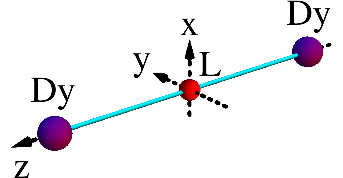
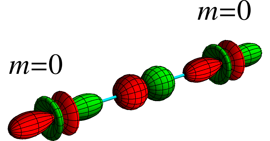
(c)

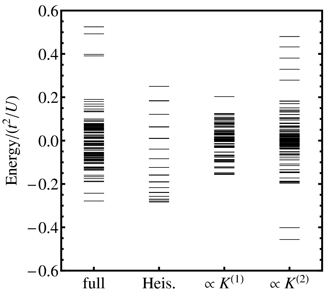
Figure 1: (Color online) (a) Linearly bridged Dy dimer with one ligand atom (L). (b) Kinetic exchange interaction between $4f_{(5z^{2}-3r^{2})z}$ orbitals. (c) Calculated exchange spectrum with full $\hat{H}_{\rm ex}$ (43) and with its different contributions ($U\equiv U_{12}=U_{21}=5$ eV). The excitation energies of the intermediate states entering Eq. (LABEL:Eq:JKE) have been calculated ab initio (Sec. V.1).

Table 2: $\mathcal{K}_{kk^{\prime}}^{(1)}$ and $\mathcal{K}_{kk^{\prime}}^{(2)}$.

$\mathcal{K}_{00}^{(1)}$	$4.4458\times 10^{-3}$	$\mathcal{K}_{11}^{(2)}$	$2.2245\times 10^{-3}$
$\mathcal{K}_{02}^{(1)}$	$-3.7903\times 10^{-3}$	$\mathcal{K}_{13}^{(2)}$	$-3.2216\times 10^{-4}$
$\mathcal{K}_{04}^{(1)}$	$1.7181\times 10^{-4}$	$\mathcal{K}_{15}^{(2)}$	$1.5888\times 10^{-5}$
$\mathcal{K}_{06}^{(1)}$	$-1.7242\times 10^{-6}$	$\mathcal{K}_{17}^{(2)}$	$-1.8049\times 10^{-7}$
$\mathcal{K}_{11}^{(1)}$	$1.0908\times 10^{-2}$	$\mathcal{K}_{22}^{(2)}$	$4.8355\times 10^{-5}$
$\mathcal{K}_{13}^{(1)}$	$-1.1514\times 10^{-3}$	$\mathcal{K}_{24}^{(2)}$	$-4.6269\times 10^{-6}$
$\mathcal{K}_{15}^{(1)}$	$3.5361\times 10^{-5}$	$\mathcal{K}_{26}^{(2)}$	$7.4785\times 10^{-8}$
$\mathcal{K}_{17}^{(1)}$	$-2.9084\times 10^{-7}$	$\mathcal{K}_{33}^{(2)}$	$4.3815\times 10^{-5}$
$\mathcal{K}_{22}^{(1)}$	$2.9710\times 10^{-3}$	$\mathcal{K}_{35}^{(2)}$	$-2.1423\times 10^{-6}$
$\mathcal{K}_{24}^{(1)}$	$-1.3026\times 10^{-4}$	$\mathcal{K}_{37}^{(2)}$	$2.3716\times 10^{-8}$
$\mathcal{K}_{26}^{(1)}$	$1.2614\times 10^{-6}$	$\mathcal{K}_{44}^{(2)}$	$4.4502\times 10^{-7}$
$\mathcal{K}_{33}^{(1)}$	$1.1745\times 10^{-4}$	$\mathcal{K}_{46}^{(2)}$	$-7.2365\times 10^{-9}$
$\mathcal{K}_{35}^{(1)}$	$-3.3571\times 10^{-6}$	$\mathcal{K}_{55}^{(2)}$	$1.0531\times 10^{-7}$
$\mathcal{K}_{37}^{(1)}$	$2.6060\times 10^{-8}$	$\mathcal{K}_{57}^{(2)}$	$-1.1732\times 10^{-9}$
$\mathcal{K}_{44}^{(1)}$	$5.4544\times 10^{-6}$	$\mathcal{K}_{66}^{(2)}$	$1.1839\times 10^{-10}$
$\mathcal{K}_{46}^{(1)}$	$-4.9672\times 10^{-8}$	$\mathcal{K}_{77}^{(2)}$	$1.3155\times 10^{-11}$
$\mathcal{K}_{55}^{(1)}$	$7.4109\times 10^{-8}$
$\mathcal{K}_{57}^{(1)}$	$-3.9138\times 10^{-10}$
$\mathcal{K}_{66}^{(1)}$	$4.1115\times 10^{-10}$

(a)	(b)	(c)	(d)
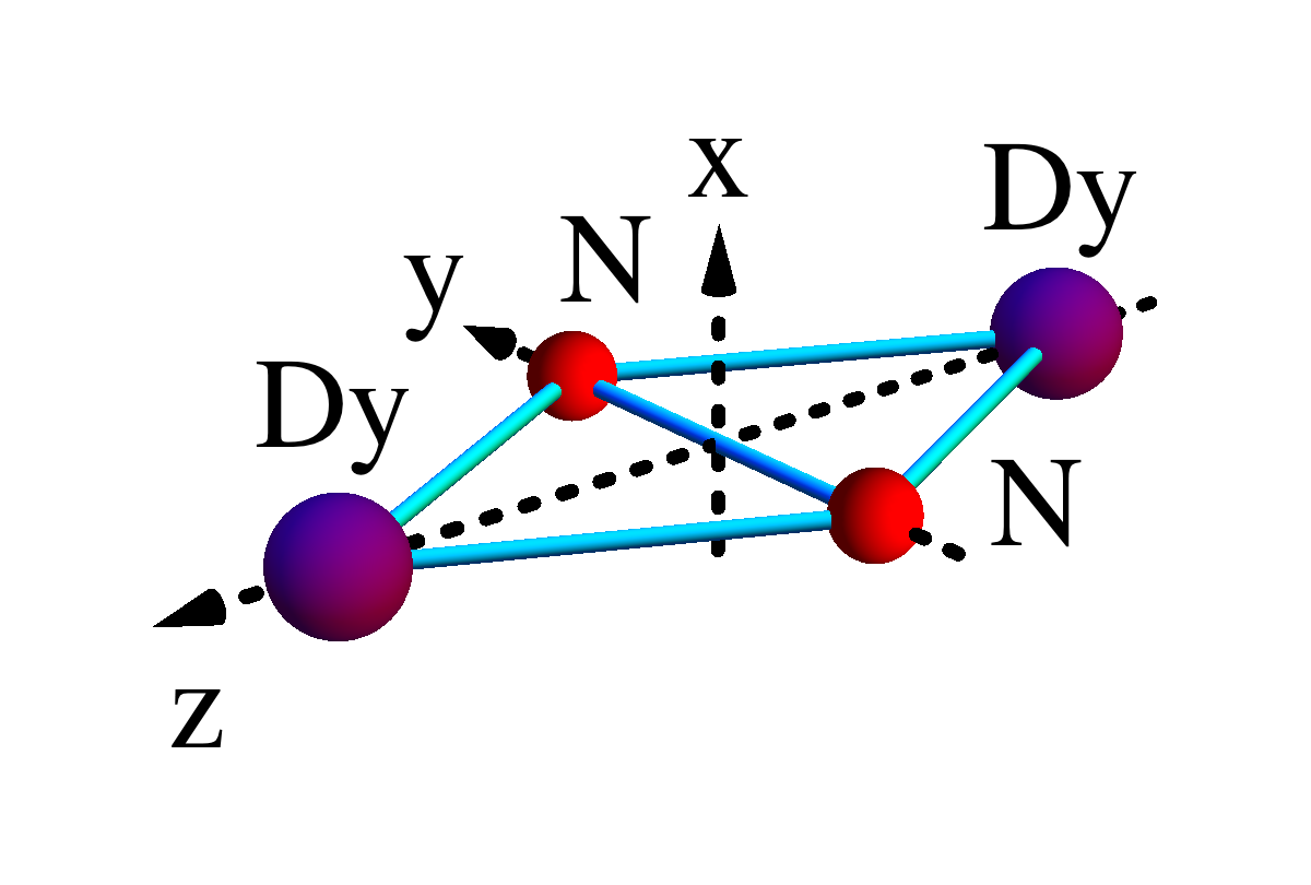
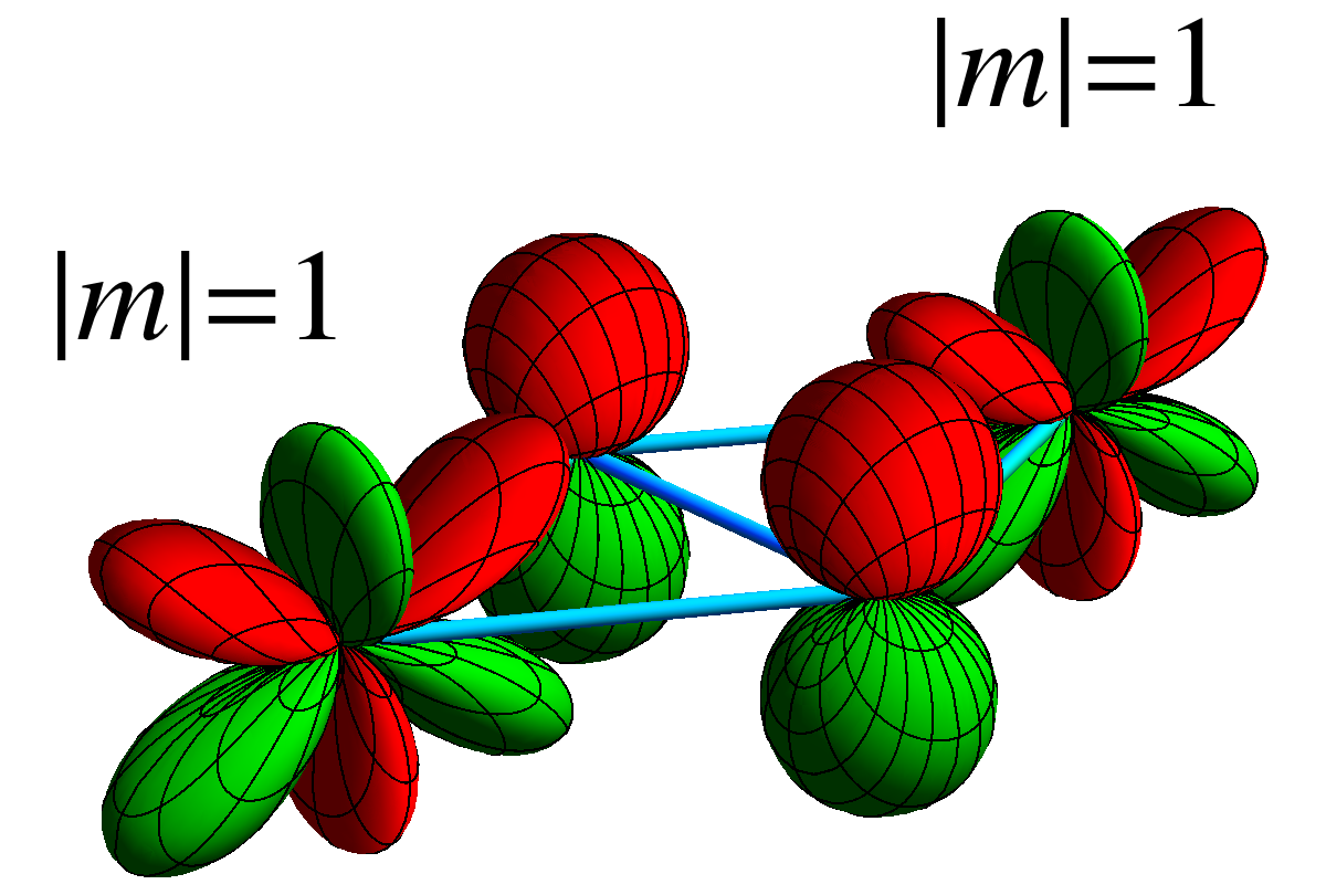
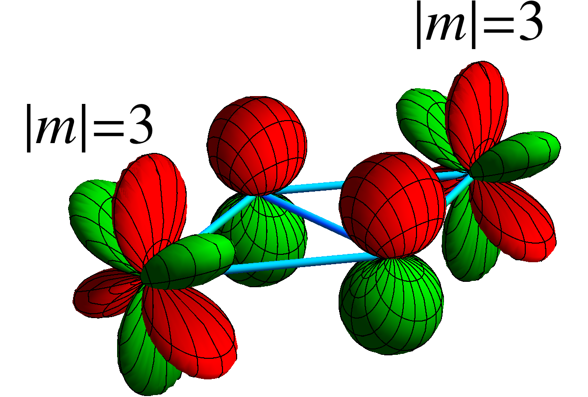
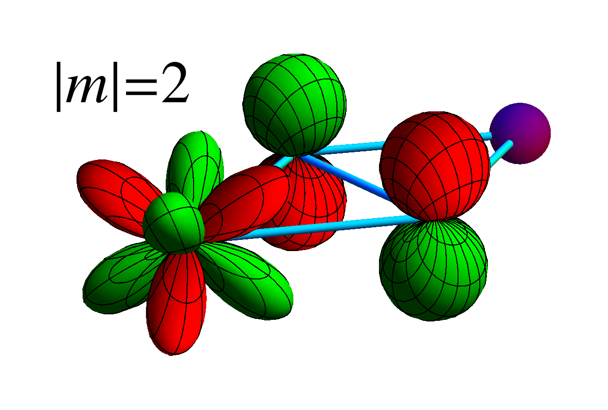
(e)		(f)

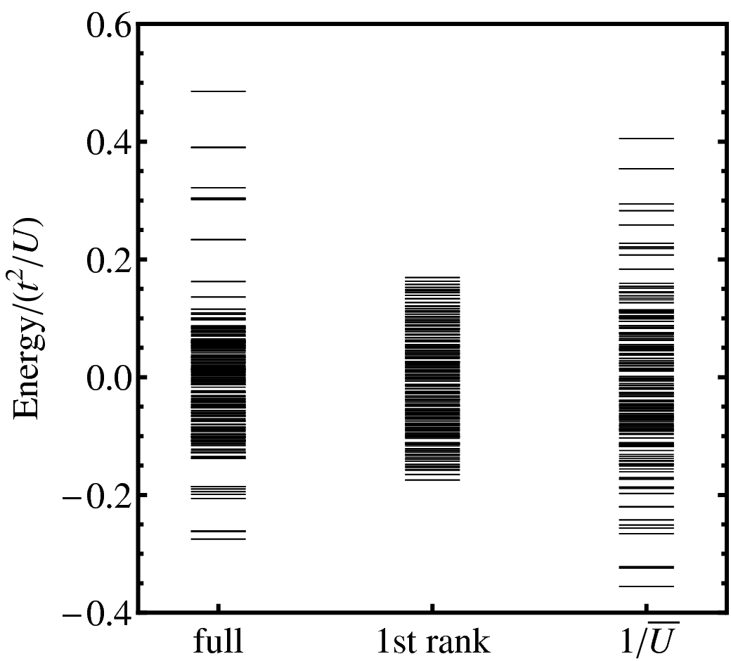
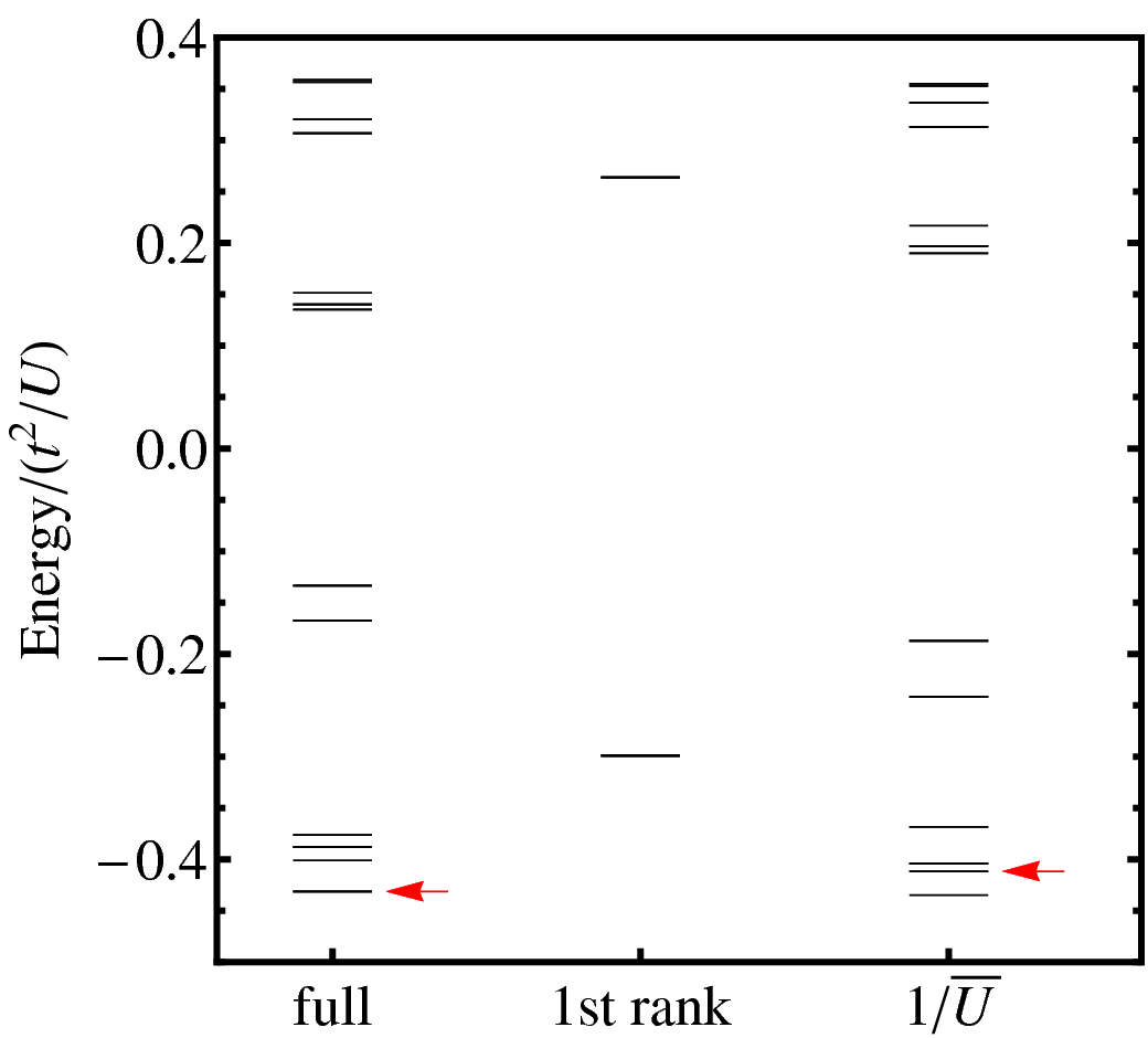
Figure 2: (Color online) (a) Dy dimer bridged via N${}_{2}^{n-}$ anion ($D_{2h}$ core symmetry). Large (purple) and small (red) balls are Dy and N, respectively. (b), (c) Kinetic exchange interaction between $4f_{(5z^{2}-r^{2})x}$ orbitals and $4f_{x^{3}-3xy^{2}}$ orbitals, respectively, via the HOMO of N${}_{2}^{2-}$. (d) Kinetic exchange interaction between the $4f_{xyz}$ orbital of Dy and the LUMO of N${}_{2}^{2-}$. (e) Calculated exchange spectrum with full $\hat{H}_{\rm ex}$ and its first-rank contribution ($U\equiv U_{12}=U_{21}=5$ eV), and in the $1/\bar{U}$ approximation for kinetic exchange pattern (b). (f) Calculated exchange spectrum with full $\hat{H}_{\rm ex}$ and its first-rank contribution ($U_{21}=$ 3 eV), and in the $1/\bar{U}$ approximation for kinetic exchange pattern (d). The calculations in (e) and (f) involved exchange parameters (LABEL:Eq:JKE) with excitation energies of the intermediate states on Dy evaluated ab initio. $\bar{U}$ in the calculation within $1/\bar{U}$ approximation was chosen to reproduce the width of the spectrum for full $\hat{H}_{\rm ex}$.

V Examples

We further consider some typical examples of $J$-$J$ and $J$-$S$ exchange interaction. Since the kinetic exchange interaction is usually much stronger than the direct exchange interaction Anderson (1959, 1963), we only take into account the former. In order to include the multiplet structure of intermediate states in Eq. (LABEL:Eq:JKE), first we calculate ab initio the excitation energies of the virtual electron-transfer states. The calculated exchange levels are compared with those arising from the bilinear form (1) and corresponding to the $1/\bar{U}$ approximation.

V.1 Excitation energies of Dy²⁺ and Dy⁴⁺ ions

The excitation energies $\Delta E_{\alpha_{J}J}$ appearing in the denominator of the kinetic exchange Hamiltonian (28) are calculated ab initio. Since the effect of the crystal-field splitting in the intermediate states is negligible (Sec. II.1), we used the energy levels of the free Ln²⁺ and Ln⁴⁺ ions. In this work, we only calculated the energies for Ln $=$ Dy that we will use in the following sections. Apart from the crystal-field splitting, there is totally symmetric electrostatic potential which only depends on the number of electrons and shifts uniformly the $J$-multiplet energies. This effect is absorbed in the minimum promotion energy $U_{ij}$ in Eq. (LABEL:Eq:JKE). The energies are calculated using the complete active space self-consistent field (CASSCF) and the restricted active space SCF state interaction (RASSI) methods with ANO-RCC QZP basis set Aquilante et al. (2010). With the CASSCF method, the $LS$-term energies are obtained, while with the RASSI method, the spin-orbit ($J$-multiplet) energy levels are calculated. For the CASSCF calculations, all $4f$ orbitals are included into the active space. The terms included in the RASSI mixing are ${}^{6}P$, ${}^{6}F$, ${}^{6}H$ for Dy²⁺ and ${}^{7}F$, ${}^{5}S$, ${}^{5}P$, three ${}^{5}D$, two ${}^{5}F$, three ${}^{5}G$, two ${}^{5}H$, two ${}^{5}I$, ${}^{5}K$, ${}^{5}L$ for Dy⁴⁺. The excitation energies are tabulated in Table 1.

There are several $LS$-terms which appear more than once, i.e., ${}^{5}D$, ${}^{5}F$, ${}^{5}G$, ${}^{5}H$, ${}^{5}I$ terms of Dy⁴⁺ ion. These terms obtained by the CASSCF calculations are assigned to the symmetrized $LS$-states within the shell model, $|l^{N}\alpha_{LS}LSJM\rangle$, comparing the patterns of the ab initio and the model spin-orbit splittings of each $LS$-term. The symmetrized $LS$-states are constructed by using the coefficient of fractional parentage Nielson and Koster (1963). In the basis of symmetrized states, the matrix element of the spin-orbit Hamiltonian $\hat{H}_{\rm so}=\zeta\sum_{i=1}^{N}\hat{\mathbf{l}}_{i}\cdot\hat{\mathbf{s}}_{i}$ $(\zeta>0)$ is given by

$$\langle l^{4l+2-N} \alpha_{LS}LSJM_{J}|\hat{H}_{\rm so}|l^{4l+2-N}\alpha_{LS}^{\prime}L^{\prime}S^{\prime}J^{\prime}M_{J}^{\prime}\rangle$$

$$=-\delta_{LL^{\prime}}\delta_{SS^{\prime}}\delta_{JJ^{\prime}}\delta_{M_{J}M_{J}^{\prime}}\zeta\frac{\Pi_{lJ}\sqrt{l(l+1)}}{\sqrt{2}}$$

$$\times\begin{Bmatrix}L&S&J\\ L&S&J\\ 1&1&0\end{Bmatrix}\langle l^{N}\alpha_{LS}LS\|\{\hat{c}^{\dagger}\otimes\bar{c}\}_{1}^{1}\|l^{N}\alpha_{LS}^{\prime}LS\rangle$$

for $N\leq 2l+1$. Here, the curly bracket with $3\times 3$ elements are the $9j$ symbol (LABEL:Eq:9j). Therefore, the spin-orbit splitting is proportional to the reduced matrix element of operator $\{\hat{c}^{\dagger}\otimes\bar{c}\}_{1-m}^{1m}$ .

V.2 Kinetic exchange through monoatomic bridge

As a simple example, consider an exchange-coupled Dy³⁺ dimer with axial bridging geometry (Fig. 1a). The largest transfer parameter ($t$) is expected between $f_{5z^{3}-3r^{2}z}$ $(m=0)$ orbitals because of their sigma bonding to the $p_{z}$ orbital of the bridging ligand atom (Fig. 1b). Then, according to the rule (38), $q_{\rm max}=1$, while Eq. (36) gives $q=-q^{\prime}$. The resulting form of the exchange Hamiltonian $\hat{H}_{\rm ex}$, after expanding the Stevens operators in Eq. (29), is

$$\hat{H}_{\rm ex} = \hat{K}^{(1)}+\hat{\mathbf{J}}_{1}\cdot\hat{\mathbf{J}}_{2}\hat{K}^{(2)}+\hat{K}^{(2)}\hat{\mathbf{J}}_{1}\cdot\hat{\mathbf{J}}_{2},$$ (43)

$$\hat{K}^{(1)} = \sum_{k,k^{\prime}=0}^{7}\mathcal{K}^{(1)}_{kk^{\prime}}\hat{J}_{1z}^{k}\hat{J}_{2z}^{k^{\prime}},$$ (44)

$$\hat{K}^{(2)} = \sum_{k,k^{\prime}=1}^{7}\mathcal{K}^{(2)}_{kk^{\prime}}\hat{J}_{1z}^{k-1}\hat{J}_{2z}^{k^{\prime}-1},$$ (45)

where $k+k^{\prime}$=even. We can see that, even in this simplest case, $\hat{H}_{\rm ex}$ does not reduce to the isotropic form (1) because Ising ($\propto\hat{K}^{(1)}$) and mixed Ising-Heisenberg ($\propto\hat{K}^{(2)}$) terms, both involving high powers of momentum projection operators of two sites. The parameters $\mathcal{K}_{kk^{\prime}}^{(1)},\mathcal{K}_{kk^{\prime}}^{(2)}$ are tabulated in Table 2. When the eigenvalue of $\hat{J}_{iz}$ is large, the higher order terms are significantly enhanced and contribute to the exchange interaction rather than the bilinear term. As a result the exchange spectra calculated with the full Hamiltonian (43) and with its Heisenberg-type part (1) show large discrepancy between them (Fig. 1(c)). The discrepancy is also seen in their eigenstates. The difference between the exchange states of (43) with those of $\hat{H}_{\text{Heis}}$ (1) is compared by expanding the former by the latter. The solution of $\hat{H}_{\text{Heis}}$ for two site system is given

$$|J_{12}M_{12}\rangle=\sum_{M_{1},M_{2}}|J_{1}M_{1},J_{2}M_{2}\rangle C_{J_{1}M_{1}J_{2}M_{2}}^{J_{12}M_{12}},$$ (46)

where $J_{12}$ and $M_{12}$ are the total angular momentum for the dimer and its projection. The low-energy exchange states of $\hat{H}_{\rm ex}$ (43) are written in the basis of $\{|J_{12}M_{12}\rangle\}$ as follows:

$$|\Psi_{1},A_{1g}\rangle \approx 0.574|0,0\rangle+0.773|2,0\rangle+0.190|4,0\rangle$$

$$- 0.160|6,0\rangle,$$

$$|\Psi_{2},A_{1u}\rangle \approx 0.846|1,0\rangle+0.505|3,0\rangle-0.161|7,0\rangle,$$

$$|\Psi_{3,4},E_{1u}\rangle \approx 0.352|1,\pm 1\rangle+0.768|3,\pm 1\rangle+0.522|5,\pm 1\rangle$$

$$+ 0.107|7,\pm 1\rangle,$$

$$|\Psi_{5,6},E_{1g}\rangle \approx 0.636|2,\pm 1\rangle+0.712|4,\pm 1\rangle+0.294|6,\pm 1\rangle.$$

Here, the irreducible representation $\Gamma$ of $D_{\infty h}$ is used, and the states $|\Psi_{i},\Gamma\rangle$ belong to the eigenvalues $E_{1,2}=-0.278523$, $E_{3,4,5,6}=-0.243015$, respectively, in the units of $t^{2}/U_{12}$. The low-energy exchange states are not necessarily mainly contributed by the ground state of the antiferromagnetic $\hat{H}_{\text{Heis}}$, $|J_{12}M_{12}\rangle=|0,0\rangle$. Therefore, we conclude that the Heisenberg form of the interaction is not adequate to describe the exchange interaction between $J$-multiplets.

(a)	(b)
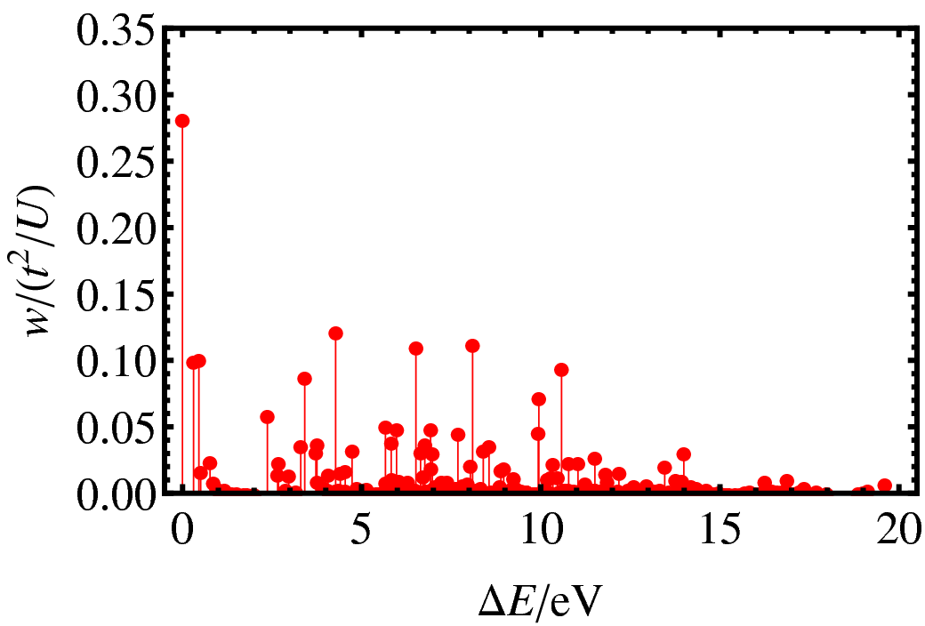
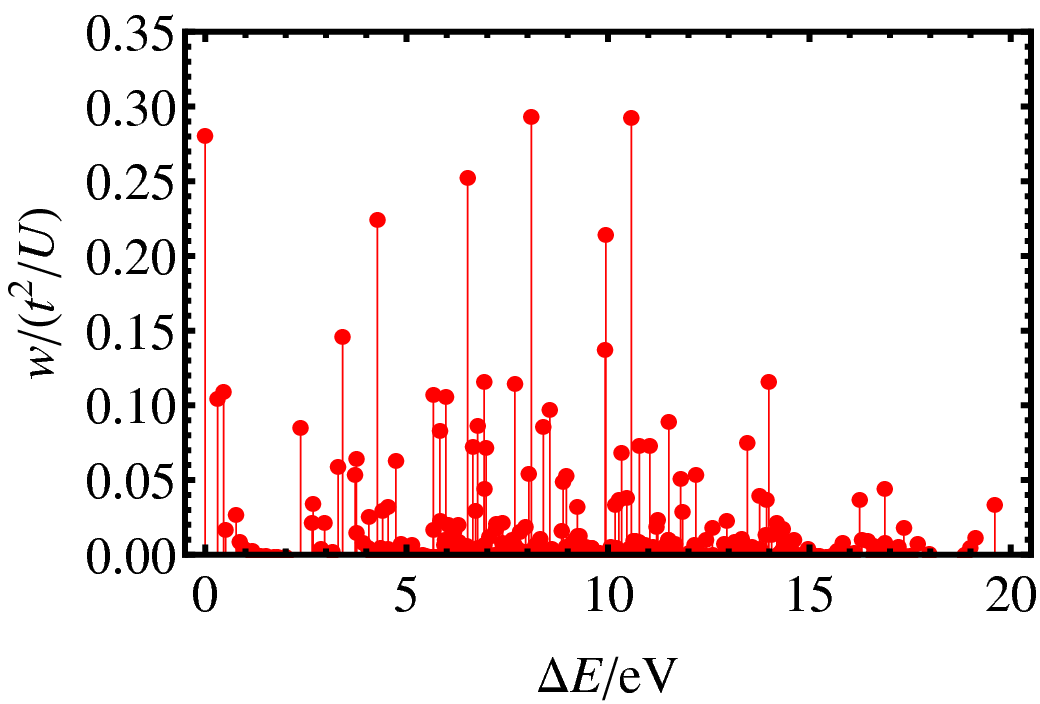
(c)	(d)

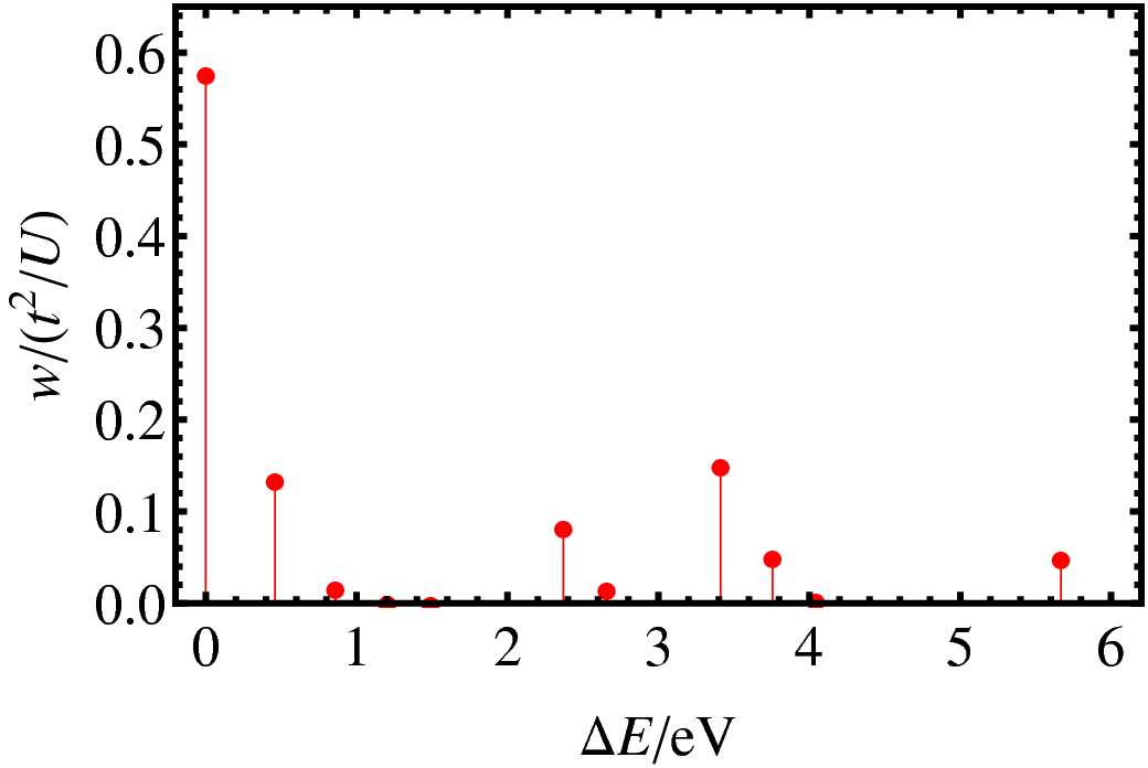
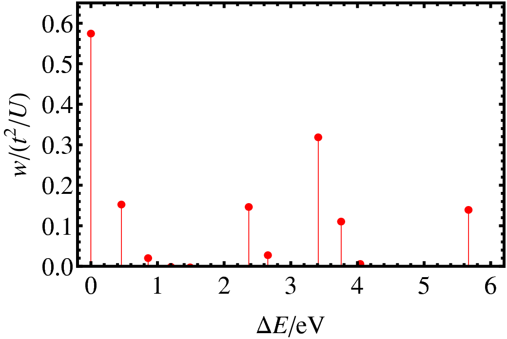
Figure 3: The contributions from the intermediate states $w$ corresponding to the excitation energy $\Delta E$ ($=\Delta E_{\alpha_{J}J}^{N}+\Delta E_{\alpha_{J}^{\prime}J^{\prime}}^{N^{\prime}}$) for (a) the full exchange interaction $\hat{H}_{\rm ex}$ and (b) the exchange within the $1/\bar{U}$ approximation $\hat{H}_{\rm ex}^{1/\bar{U}}$ for Dy³⁺ dimer bridged by N${}_{2}^{2-}$ and for (c) the full exchange interaction and (d) the exchange within the $1/\bar{U}$ approximation for the Dy-radical system ($n=3$). The units of $w$ are $t^{2}/U_{21}$ for (a), (c) and $t^{2}/\bar{U}$ for (b), (d).

V.3 Kinetic exchange through biatomic bridge

Consider the exchange interaction in the Dy³⁺ dimer bridged by the N${}_{2}^{n-}$ $(n=2,3)$ anion (Fig. 2(a)) Rinehart et al. (2011). In the case of $n=2$, $4f$ electrons of Dy³⁺ ions would transfer between the metal sites via the highest occupied molecular orbital (HOMO) of N${}_{2}^{2-}$ (Figs. 2(b),(c)). The HOMO overlaps with the $f_{(5z^{2}-r^{2})x}$ ($|m|=1$) and the $f_{x^{3}-3xy^{2}}$ ($|m|=3$) metal orbitals, the former interaction being dominant. Hence, we only consider the electron transfer between the orbitals with $|m|=1$ (Fig. 2(b)). For them $\Delta_{\rm max}=2$ and we obtain according to Eq. (38) $q_{\rm max}=3$. Then $\hat{H}_{\rm ex}$ will include powers of $\hat{J}_{i\pm}$ $(=\hat{J}_{ix}\pm i\hat{J}_{iy})$ for each center up to third order.

Figure 2(e) shows the calculated exchange spectrum for full $\hat{H}_{\rm ex}$, and its first-rank contribution, and for one single promotion energy $\bar{U}$ ($1/\bar{U}$ approximation) Elliott and Thorpe (1968); Santini et al. (2009). Although the first-rank contribution is bilinear in $\hat{J}_{i\gamma}$, it is not isotropic and the corresponding spectrum does not resemble the pattern of levels of Heisenberg-type Hamiltonian (1). Also the spectrum is quite different when the $1/\bar{U}$ approximation is applied. This approximation neglects the splitting of the $LS$-terms which exceeds several times the minimal electron promotion energy. As a result, the relative contributions to the exchange interaction from various intermediate states are significantly modified. In order to see the variation of the contributions from the intermediate states to the kinetic exchange interaction, we divide the kinetic exchange Hamiltonian as follows:

$$\hat{H}_{\text{ex}} = \sum_{\alpha_{J}J}\sum_{\alpha_{J}^{\prime}J^{\prime}}\hat{h}_{\text{ex}}(\alpha_{J}J,\alpha_{J}^{\prime}J^{\prime}).$$ (47)

Here, $\hat{h}_{\text{ex}}(\alpha_{J}J,\alpha_{J}^{\prime}J^{\prime})$ indicates the term which only includes the contribution from the set of the intermediate states $(\alpha_{J}J,\alpha_{J}^{\prime}J^{\prime})$. The contribution from each such process can be measured by the width $w$ of the eigenvalues of $\hat{h}_{\text{ex}}(\alpha_{J}J,\alpha_{J}^{\prime}J^{\prime})$. The widths $w$ for the full exchange Hamiltonian $\hat{H}_{\text{ex}}$ and those within $1/\bar{U}$ approximation are shown in Figure 3(a) and (b), respectively. In comparison with the contributions to the full Hamiltonian, those from the high energy states ($\Delta E\approx$ 5-10 eV) are exaggerated in $\hat{H}_{\text{ex}}^{1/\bar{U}}$.

In the case of N${}_{2}^{3-}$ bridge, the main exchange coupling arises between the $f_{xyz}$ orbital of Dy and the unpaired electron occupying the lowest unoccupied molecular orbital (LUMO) of N${}_{2}^{2-}$ (Fig. 2(d)). The LUMO level in N${}_{2}^{3-}$ has significantly higher energy compared to the orbital energy of $4f$ electrons in Dy³⁺. On this reason and also due to a larger space distribution of the LUMO compared to the $4f$ orbitals, the minimal electron promotion energy from N${}_{2}^{3-}$ to Dy³⁺ ($U_{21}$) is expected to be much smaller than in the opposite direction ($U_{12}$). Hence, we neglect the latter process. Given that the Dy orbitals involved in the electron transfer have $|m|=2$, according to Eq. (38) $q_{\rm max}=5$, the same for the maximal power of $\hat{J}_{1\pm}$ in the exchange Hamiltonian.

Figure 2(f) shows the exchange levels obtained for full $\hat{H}_{\rm ex}$, its first-rank part, and for the $1/\bar{U}$ approximation. In the present case, the first-rank part of $\hat{H}_{\rm ex}$ coincides with Eq. (1), while the corresponding spectrum strongly differs from the full $\hat{H}_{\rm ex}$ indicating the importance of higher order terms. As in the previous example, the $1/\bar{U}$ approximation modifies the relative contributions to the exchange interaction from intermediate states (Fig. 3 (c),(d)) and induces, in particular, the interchange of the three-fold degenerate ground and the nondegenerate first excited states (marked with arrow in Fig. 2(f)) . Because of the difference in the nature of the exchange states, the magnetic properties predicted by the exchange states of the full Hamiltonian and the $1/\bar{U}$ approximation differ from each other.

There is another reason that the $1/\bar{U}$ approximation is not recommended: the Hund’s rule coupling is completely neglected within this approximation, leading to the removal of the Goodenough’s ferromagnetic exchange contribution Goodenough (1963) though the latter plays important role in many systems.

VI Conclusion

The main results of the present work can be summarized as follows:

1. We derived the Hamiltonian of exchange interaction between $J$-multiplets ($J$-$J$) and between $J$-multiplet and isotropic spin ($J$-$S$) on the basis of a complete electronic Hamiltonian, including the intrasite relativistic effects. The exchange parameters are expressed via microscopic quantities which can be extracted from first principle calculations. Despite their microscopic character, the obtained expressions (33) and (LABEL:Eq:JKE) are general (i) for arbitrary choice of quantization axes on two magnetic sites (which are not expected to coincide) and (ii) for various magnetic ions, which can be lanthanides, actinides, transition metal ions under special conditions or any their combinations. The only requirement is that the low-lying states on the sites are well approximated by crystal-field split eigenstates of a total angular momentum.

2. The structure of the $J$-$J$ and $J$-$S$ exchange Hamiltonian is clarified on the basis of derived exchange Hamiltonian. More specific, the maximal rank and the projections of the irreducible tensors appearing in the exchange Hamiltonian are elucidated.

3. The obtained form of the (kinetic) exchange Hamiltonian was analyzed for different geometries of the bridge. The relation between the geometry and the structure of the Hamiltonian was established.

4. On the basis of considered examples, we found that the exchange spectrum in systems with $J$-$J$ and $J$-$S$ interaction cannot be adequately described neither by exchange Hamiltonian of isotropic form (1) nor within the $1/\bar{U}$ approximation.

5. The contributions to the kinetic exchange Hamiltonian from the intermediate $J$-multiplets are analyzed. It is found that the $1/\bar{U}$ approximation exaggerates the terms from the excited states. Moreover, within the $1/\bar{U}$ approximation, the term splitting which is larger than the average $U$ is neglected, leading to the wrong order of exchange levels.

In combination with ab initio and DFT extraction of microscopic electronic parameters, the microscopic exchange Hamiltonians derived in this work can become a powerful tool for the investigation of strongly anisotropic materials containing metal ions with unquenched orbital momentum.

Appendix A Theoretical tools

The transformation of the exchange Hamiltonian into the tensor form is done using the theory of angular momentum Judd (1967); Edmonds (1974); Varshalovich et al. (1988). For the convenience of the readers, the tools necessary in the derivation are collected here.

A.1 Coupling of angular momenta

For the phase of the spherical harmonics $Y_{j}^{m}(\theta,\phi)$, we use the convention in Refs. Edmonds, 1974; Varshalovich et al., 1988. With this phase convention, the complex conjugation of $Y_{j}^{m}$ is related to $Y_{j}^{-m}$ as

$$\left[Y_{j}^{m}(\theta,\phi)\right]^{*} = (-1)^{m}Y_{j}^{-m}(\theta,\phi).$$ (48)

Here, the subscript $j$ indicates the rank, the superscript $m$ is the component, $\theta$ and $\phi$ are the spherical angular coordinates.

Consider two systems whose states are the eigenstates of the angular momentum, $|j_{i}m_{i}\rangle$ $(i=1,2)$. The coupled state characterized by the total angular momentum can be constructed using the Clebsch-Gordan coefficients, $C_{j_{1}m_{1}j_{2}m_{2}}^{jm}$:

$$|jm\rangle = \sum_{m_{1},m_{2}}|j_{1}m_{1},j_{2}m_{2}\rangle C_{j_{1}m_{1}j_{2}m_{2}}^{jm}.$$ (49)

The Clebsch-Gordan coefficients have following symmetry properties (Eqs. 8.4.3. (10), (11) in Ref. Varshalovich et al., 1988):

$$C_{j_{1}m_{1}j_{2}m_{2}}^{j_{3}m_{3}} = (-1)^{j_{1}+j_{2}-j_{3}}C_{j_{2}m_{2}j_{1}m_{1}}^{j_{3}m_{3}}$$ (50)

$$= (-1)^{j_{1}-m_{1}}\frac{\Pi_{j_{3}}}{\Pi_{j_{2}}}C_{j_{1}m_{1}j_{3}-m_{3}}^{j_{2}-m_{2}}$$

$$= (-1)^{j_{1}-m_{1}}\frac{\Pi_{j_{3}}}{\Pi_{j_{2}}}C_{j_{3}m_{3}j_{1}-m_{1}}^{j_{2}m_{2}}$$

$$= (-1)^{j_{2}+m_{2}}\frac{\Pi_{j_{3}}}{\Pi_{j_{1}}}C_{j_{3}-m_{3}j_{2}m_{2}}^{j_{1}-m_{1}}$$

$$= (-1)^{j_{2}+m_{2}}\frac{\Pi_{j_{3}}}{\Pi_{j_{1}}}C_{j_{2}-m_{2}j_{3}m_{3}}^{j_{1}m_{1}}$$

$$= (-1)^{j_{1}+j_{2}-j_{3}}C_{j_{1}-m_{1}j_{2}-m_{2}}^{j_{3}-m_{3}},$$

where $\Pi_{j}=\sqrt{2j+1}$.

Using the Clebsch-Gordan coefficients, the $6j$ and $9j$ symbols are defined as Varshalovich et al. (1988)

$$\delta_{jj^{\prime}}\delta_{mm^{\prime}}(-1)^{j_{1}+j_{2}+j_{3}+j}\Pi_{j_{12}j_{23}}\begin{Bmatrix}j_{1}&j_{2}&j_{12}\\ j_{3}&j&j_{23}\end{Bmatrix} = \sum_{m_{i}m_{ij}}C_{j_{12}m_{12}j_{3}m_{3}}^{jm}C_{j_{1}m_{1}j_{2}m_{2}}^{j_{12}m_{12}}C_{j_{1}m_{1}j_{23}m_{23}}^{j^{\prime}m^{\prime}}C_{j_{2}m_{2}j_{3}m_{3}}^{j_{23}m_{23}},$$ (51)

and

$$\delta_{jj^{\prime}}\delta_{mm^{\prime}}\Pi_{j_{12}j_{34}j_{13}j_{24}}\begin{Bmatrix}j_{1}&j_{2}&j_{12}\\ j_{3}&j_{4}&j_{34}\\ j_{13}&j_{24}&j\end{Bmatrix} = \sum_{m_{i}m_{ij}}C_{j_{12}m_{12}j_{34}m_{34}}^{jm}C_{j_{1}m_{1}j_{2}m_{2}}^{j_{12}m_{12}}C_{j_{3}m_{3}j_{4}m_{4}}^{j_{34}m_{34}}C_{j_{13}m_{13}j_{24}m_{24}}^{j^{\prime}m^{\prime}}C_{j_{1}m_{1}j_{3}m_{3}}^{j_{13}m_{13}}C_{j_{2}m_{2}j_{4}m_{4}}^{j_{24}m_{24}},$$

respectively. Here, $\sum_{m_{i},m_{ij}}$ stands for the summation over all $m_{i}$ and $m_{ij}$ ($i,j=1,2,3,4$). The $6j$ symbol (51) is symmetric with respect to the permutation of columns and the interchange of the upper and lower components of two columns (Eq. 9.4.2. (2) in Ref. Varshalovich et al., 1988).

From Eqs. (51), (LABEL:Eq:9j), we immediately obtain some formulae involving $6j$ or $9j$ symbol. Multiplying both sides of Eq. (51) by $C_{j_{1}m_{1}j_{23}m_{23}}^{j^{\prime}m^{\prime}}$ and summing over $j^{\prime}m^{\prime}$, we obtain (Eq. 8.7.3. (12) in Ref. Varshalovich et al., 1988)

$$(-1)^{j_{1}+j_{2}+j_{3}+j}\Pi_{j_{12}j_{23}}C_{j_{1}m_{1}j_{23}m_{23}}^{jm}\begin{Bmatrix}j_{1}&j_{2}&j_{12}\\ j_{3}&j&j_{23}\end{Bmatrix} = \sum_{m_{2}m_{3}m_{12}}C_{j_{12}m_{12}j_{3}m_{3}}^{jm}C_{j_{1}m_{1}j_{2}m_{2}}^{j_{12}m_{12}}C_{j_{2}m_{2}j_{3}m_{3}}^{j_{23}m_{23}}.$$ (53)

Similarly, multiplying both sides of Eq. (51) by $C_{j_{12}m_{12}j_{3}m_{3}}^{jm}C_{j_{1}m_{1}j_{23}m_{23}}^{j^{\prime}m^{\prime}}$ and summing over $jm,j^{\prime}m^{\prime}$, we obtain (Eq. 8.7.3. (12) in Ref. Varshalovich et al., 1988)

$$\sum_{jm}(-1)^{j_{1}+j_{2}+j_{3}+j}\Pi_{j_{12}j_{23}}C_{j_{12}m_{12}j_{3}m_{3}}^{jm}C_{j_{1}m_{1}j_{23}m_{23}}^{jm}\begin{Bmatrix}j_{1}&j_{2}&j_{12}\\ j_{3}&j&j_{23}\end{Bmatrix} = \sum_{m_{2}}C_{j_{1}m_{1}j_{2}m_{2}}^{j_{12}m_{12}}C_{j_{2}m_{2}j_{3}m_{3}}^{j_{23}m_{23}}.$$ (54)

Multiplying both sides of Eq. (LABEL:Eq:9j) by $C_{j_{13}m_{13}j_{24}m_{24}}^{j^{\prime}m^{\prime}}$ and summing over $j^{\prime}m^{\prime}$, we obtain similar formula involving five Clebsch-Gordan coefficients:

$$\Pi_{j_{12}j_{34}j_{13}j_{24}}C_{j_{13}m_{13}j_{24}m_{24}}^{jm}\begin{Bmatrix}j_{1}&j_{2}&j_{12}\\ j_{3}&j_{4}&j_{34}\\ j_{13}&j_{24}&j\end{Bmatrix} = \sum_{m_{i}m_{ij}}C_{j_{12}m_{12}j_{34}m_{34}}^{jm}C_{j_{1}m_{1}j_{2}m_{2}}^{j_{12}m_{12}}C_{j_{3}m_{3}j_{4}m_{4}}^{j_{34}m_{34}}C_{j_{1}m_{1}j_{3}m_{3}}^{j_{13}m_{13}}C_{j_{2}m_{2}j_{4}m_{4}}^{j_{24}m_{24}}.$$ (55)

Multiplying both sides of Eq. (LABEL:Eq:9j) by $C_{j_{12}m_{12}j_{34}m_{34}}^{jm}C_{j_{13}m_{13}j_{24}m_{24}}^{j^{\prime}m^{\prime}}$ and summing over $jm,j^{\prime}m^{\prime}$, we obtain a formula involving five Clebsch-Gordan coefficients (Eq. 8.7.4. (26) in Ref. Varshalovich et al., 1988):

$$\Pi_{j_{12}j_{34}j_{13}j_{24}}\sum_{jm}C_{j_{12}m_{12}j_{34}m_{34}}^{jm}C_{j_{13}m_{13}j_{24}m_{24}}^{jm}\begin{Bmatrix}j_{1}&j_{2}&j_{12}\\ j_{3}&j_{4}&j_{34}\\ j_{13}&j_{24}&j\end{Bmatrix} = \sum_{m_{i}}C_{j_{1}m_{1}j_{2}m_{2}}^{j_{12}m_{12}}C_{j_{3}m_{3}j_{4}m_{4}}^{j_{34}m_{34}}C_{j_{1}m_{1}j_{3}m_{3}}^{j_{13}m_{13}}C_{j_{2}m_{2}j_{4}m_{4}}^{j_{24}m_{24}}.$$ (56)

A.2 Irreducible tensor operator

The irreducible tensor operator is defined as the operator $\hat{T}_{kq}$ which transforms as spherical harmonics $Y_{k}^{q}$ (48) under $SO(3)$ rotations:

$$\hat{R}\hat{T}_{kq}\hat{R}^{\dagger} = \sum_{q^{\prime}=-k}^{k}\hat{T}_{kq^{\prime}}D_{q^{\prime}q}^{k}(R),$$ (57)

where $D_{q^{\prime}q}^{k}(R)=\langle Y_{k}^{q^{\prime}}|\hat{R}|Y_{k}^{q}\rangle$ is the Wigner $D$-function Varshalovich et al. (1988), $R\in SO(3)$, and $\hat{R}$ is the rotational operator for $R$. Since Eq. (57) holds for any infinitesimal rotations, $\hat{T}_{kq}$ satisfies

$$\left[\hat{J}_{\mu},\hat{T}_{kq}\right] = \sqrt{k(k+1)}C_{kq1\mu}^{kq+\mu}\hat{T}_{kq+\mu}.$$ (58)

The matrix element of $\hat{T}_{kq}$ with respect to the eigenstates of the angular momentum, $\{|JM\rangle\}$, is proportional to the Clebsch-Gordan coefficient (49). The Wigner-Eckart theorem reads (Eq. 13.1.1. (2) in Ref. Varshalovich et al., 1988)

$$\langle JM^{\prime}|\hat{T}_{kq}|JM\rangle = \frac{(-1)^{2k}\langle J\|\hat{T}_{k}\|J\rangle}{\Pi_{J}}C_{JMkq}^{JM^{\prime}}.$$ (59)

One of the irreducible tensor operators is the spherical tensor operator $Y_{k}^{q}(\hat{\mathbf{J}})$ which is constructed replacing the coordinates in the spherical harmonics $Y_{k}^{q}(\mathbf{r}/r)$ by the total angular momentum operator ($\mathbf{r}/r\rightarrow\hat{\mathbf{J}}$) and averaging it over all possible permutations of $\hat{\mathbf{J}}$ operators Abragam and Bleaney (1970). For example, $\hat{J}_{\mu}\hat{J}_{\nu}$ is replaced by $(\hat{J}_{\mu}\hat{J}_{\nu}+\hat{J}_{\nu}\hat{J}_{\mu})/2$.

When the system consists of two subsystems, double tensor Judd (1967); Varshalovich et al. (1988) is used. In this work, the subsystems are the orbital and the spin parts of the system. The orbital and spin subsystems transform as irreducible tensor within $SO(3)$ and $SU(2)$ operations, respectively. Thus, for the rotation of the system $R=R_{1}R_{2}\in SO(3)\otimes SU(2)$, where $R_{1}\in SO(3)$ and $R_{2}\in SU(2)$, the double tensor $\hat{T}^{k_{1}q_{1}}_{k_{2}q_{2}}$ of ranks $k_{1}$ and $k_{2}$ transform as

$$\hat{R}\hat{T}^{k_{1}q_{1}}_{k_{2}q_{2}}\hat{R}^{\dagger} = \sum_{q_{1}^{\prime}=-k_{1}}^{k_{1}}\sum_{q_{2}^{\prime}=-k_{2}}^{k_{2}}\hat{T}^{k_{1}q_{1}^{\prime}}_{k_{2}q_{2}^{\prime}}D_{q_{1}^{\prime}q_{1}}^{k_{1}}(R_{1})D_{q_{2}^{\prime}q_{2}}^{k_{2}}(R_{2}),$$

and $\hat{T}^{k_{1}q_{1}}_{k_{2}q_{2}}$ fulfills

$$\left[\hat{L}_{\mu},\hat{T}^{k_{1}q_{1}}_{k_{2}q_{2}}\right] = \sqrt{k_{1}(k_{1}+1)}C_{k_{1}q_{1}1\mu}^{k_{1}q_{1}+\mu}\hat{T}^{k_{1}q_{1}+\mu}_{k_{2}q_{2}},$$ (61)

$$\left[\hat{S}_{\mu},\hat{T}^{k_{1}q_{1}}_{k_{2}q_{2}}\right] = \sqrt{k_{2}(k_{2}+1)}C_{k_{2}q_{2}1\mu}^{k_{2}q_{2}+\mu}\hat{T}^{k_{1}q_{1}}_{k_{2}q_{2}+\mu}.$$ (62)

One of the double tensor operator is the electron creation operator in atomic spin-orbital $(m,\sigma)$, $\hat{c}_{im\sigma}^{\dagger}$. This is clear since $\hat{c}_{im\sigma}^{\dagger}$ creates the one-electron state which transforms as the product of the spherical harmonics, $|lm,\frac{1}{2}\sigma\rangle$. On the other hand, the annihilation operator $\hat{c}_{im\sigma}$ does not fulfill Eqs. (61) and (62), whereas $\bar{c}_{i-m-\sigma}$ defined below does Judd (1967):

$$\hat{c}_{im\sigma} = (-1)^{l_{i}+m+\frac{1}{2}+\sigma}\bar{c}_{i-m-\sigma}.$$ (63)

Thus, $\bar{c}_{i-m-\sigma}$ instead of the annihilation operator is a double tensor.

A.3 Method of equivalent operator

Consider an irreducible tensor $\hat{T}_{kq}$ of rank $k$ and its argument $q$ acting on the spin degrees of freedom. Replacing $J$ in Eq. (59) with $S$, we obtain an expression of the matrix element of $\hat{T}_{kq}$. On the other hand, the matrix element of the spherical tensor operator $Y_{k}^{q}(\hat{\mathbf{S}})$ is written as

$$\langle SM^{\prime}|Y_{k}^{q}(\hat{\mathbf{S}})|SM\rangle = \frac{(-1)^{2k}\langle S\|Y_{k}(\hat{\mathbf{S}})\|S\rangle}{\Pi_{S}}C_{SMkq}^{SM^{\prime}},$$

where $\hat{\mathbf{S}}$ is an abstract spin operator. Comparing Eqs. (59) and (LABEL:Eq:Ymat), one finds the relation between tensor operators $\hat{T}_{kq}$ and $Y_{k}^{q}(\hat{\mathbf{S}})$:

$$\langle SM^{\prime}|\hat{T}_{kq}|SM\rangle = \frac{\langle S\|\hat{T}_{k}\|S\rangle}{\langle S\|Y_{k}(\hat{\mathbf{S}})\|S\rangle}\langle SM^{\prime}|Y_{k}^{q}(\hat{\mathbf{S}})|SM\rangle.$$

This equation holds for any matrix element, and hence, in the space of $\{|SM\rangle\}$,

$$\hat{T}_{kq} = \frac{\langle S\|\hat{T}_{k}\|S\rangle}{\langle S\|Y_{k}(\hat{\mathbf{S}})\|S\rangle}Y_{k}^{q}(\hat{\mathbf{S}}).$$ (66)

The reduced matrix element in the denominator is simplified using Eq. (LABEL:Eq:Ymat) with $M=M^{\prime}=S$ and $q=0$,

$${\langle S\|Y_{k}(\hat{\mathbf{S}})\|S\rangle} = \frac{(-1)^{-2k}\Pi_{S}}{C_{SSk0}^{SS}}Y_{k}^{0}(S).$$ (67)

Consequently, $\hat{T}_{kq}$ is expressed as

$$\hat{T}_{kq} = \frac{(-1)^{2k}\langle S\|\hat{T}_{k}\|S\rangle}{\Pi_{S}}C_{SSk0}^{SS}\frac{Y_{k}^{q}(\hat{\mathbf{S}})}{Y_{k}^{0}(S)}.$$ (68)

Eq. (68) holds for

$$0\leq k\leq 2S.$$ (69)

$Y_{k}^{q}(S)$ in the denominator of Eq. (68) is the scalar obtained by substituting $\hat{\mathbf{S}}^{2}=S(S+1)$ and $\hat{S}_{z}=S$ in the spherical harmonic tensor $Y_{k}^{q}(\hat{\mathbf{S}})$.

Now, we consider the case of double tensors $\hat{T}^{kq}_{k^{\prime}q^{\prime}}$ of rank $(k,k^{\prime})$. Assuming Eq. (2), it is transformed into the tensor form within the space of the ground $J$-multiplet, $\{|JM\rangle\}$. The matrix element of $\hat{T}^{kq}_{k^{\prime}q^{\prime}}$ is

$$\langle JM^{\prime}|\hat{T}^{kq}_{k^{\prime}q^{\prime}}|JM\rangle = \sum_{M_{L}^{\prime}M_{S}^{\prime}}\sum_{M_{L}M_{S}}C_{LM_{L}^{\prime}SM_{S}^{\prime}}^{JM^{\prime}}C_{LM_{L}SM_{S}}^{JM}$$

$$\times \langle LM_{L}^{\prime}SM_{S}^{\prime}|\hat{T}^{kq}_{k^{\prime}q^{\prime}}|LM_{L}SM_{S}\rangle.$$

The Wigner-Eckart theorem (59) is applied to the orbital and the spin parts of the double tensor separately,

$$\langle JM^{\prime}|\hat{T}^{kq}_{k^{\prime}q^{\prime}}|JM\rangle = \frac{(-1)^{2k+2k^{\prime}}\langle LS\|\hat{T}^{k}_{k^{\prime}}\|LS\rangle}{\Pi_{LS}}$$ (71)

$$\times \sum_{M_{L}^{\prime}M_{S}^{\prime}}\sum_{M_{L}M_{S}}C_{LM_{L}^{\prime}SM_{S}^{\prime}}^{JM^{\prime}}C_{LM_{L}SM_{S}}^{JM}$$

$$\times C_{LM_{L}kq}^{LM_{L}^{\prime}}C_{SM_{S}k^{\prime}q^{\prime}}^{SM_{S}^{\prime}}.$$

Using Eq. (56), the sum of the products of the Clebsch-Gordan coefficients reduces to the sum involving $9j$ symbol:

$$\langle JM^{\prime}|\hat{T}^{kq}_{k^{\prime}q^{\prime}}|JM\rangle = (-1)^{2k+2k^{\prime}}\langle LS\|\hat{T}^{k}_{k^{\prime}}\|LS\rangle\sum_{nm}\Pi_{Jn}$$ (72)

$$\times C_{JMnm}^{JM^{\prime}}C_{kqk^{\prime}q^{\prime}}^{nm}\begin{Bmatrix}L&S&J\\ L&S&J\\ k&k^{\prime}&n\end{Bmatrix},$$

where $n$ is the rank, $m$ is its argument. The rest procedure is the same as the derivation of Eq. (68). $C_{JMnm}^{JM^{\prime}}$ is replaced by the matrix element of the irreducible tensor operator $Y_{n}^{m}(\hat{\mathbf{J}})$, and $\hat{T}^{kq}_{k^{\prime}q^{\prime}}$ within $\{|JM\rangle\}$ is expressed as

$$\hat{T}^{kq}_{k^{\prime}q^{\prime}} = (-1)^{2k+2k^{\prime}}\langle LS\|\hat{T}^{k}_{k^{\prime}}\|LS\rangle\sum_{nm}\Pi_{Jn}$$ (73)

$$\times C_{JJn0}^{JJ}C_{kqk^{\prime}q^{\prime}}^{nm}\begin{Bmatrix}L&S&J\\ L&S&J\\ k&k^{\prime}&n\end{Bmatrix}\frac{Y_{n}^{m}(\hat{\mathbf{J}})}{Y_{n}^{0}(J)}.$$

$k$, $k^{\prime}$, and $n$ in Eq. (73) obey

$$0\leq k\leq 2L,\quad 0\leq k^{\prime}\leq 2S,$$

$$\max[|k-k^{\prime}|,0]\leq n\leq\min[k+k^{\prime},2J].$$ (74)

In the derivation of Eq. (73) we used Eq. (2), while it is not mandatory. However, without using Eq. (2), the result will have a more complicated form.

In the previous works, the so-called Stevens operator $O_{k}^{q}(\hat{\mathbf{J}})=A_{kq}Y_{k}^{q}(\hat{\mathbf{J}})$ has been used instead of $Y_{k}^{q}$ where $A_{kq}$ is a coefficient which depends on both $k$ and $q$ Stevens (1952). However, the original Stevens operator does neither obey Eq. (58) nor the Wigner-Eckart theorem (59). In order to use the Wigner-Eckart theorem, one can introduce such coefficient $A_{k}$ that only depends on $k$ and is independent from $q$ Chibotaru and Ungur (2012); Chibotaru (2013). Furthermore, we write the Stevens operator in the form of $O_{k}^{q}(\hat{\mathbf{J}})/O_{k}^{0}(J)$ which is equal to $Y_{k}^{q}(\hat{\mathbf{J}})/Y_{k}^{0}(J)$. Since the constant $A_{k}$ is canceled in this form, it is possible to apply the Wigner-Eckart theorem (59):

$$\langle JM^{\prime}|\frac{O_{k}^{q}(\hat{\mathbf{J}})}{O_{k}^{0}(J)}|JM\rangle = \frac{C_{JMkq}^{JM^{\prime}}}{C_{JJk0}^{JJ}}.$$ (75)

In this article, we use the latter (see for example Eq. (73)).

Appendix B Derivation of the exchange Hamiltonian in $J$-representation

B.1 Direct exchange Hamiltonian

Detailed calculation of $\mathcal{J}^{\text{DE}}$ is shown here. Applying the method of equivalent operator (73), $\{\hat{c}_{i}^{\dagger}\otimes\bar{c}_{i}\}^{a\alpha}_{b\beta}$ in Eq. (31) becomes

$$\left\{\hat{c}_{i}^{\dagger}\otimes\bar{c}_{i}\right\}^{a\alpha}_{b\beta} = \sum_{kq}\Pi_{kJ_{i}}C_{J_{i}J_{i}k0}^{J_{i}J_{i}}C_{a\alpha b\beta}^{kq}\begin{Bmatrix}L_{i}&S_{i}&J_{i}\\ L_{i}&S_{i}&J_{i}\\ a&b&k\\ \end{Bmatrix}$$ (76)

$$\times (-1)^{2a+2b}\langle L_{i}S_{i}\|\left\{\hat{c}_{i}^{\dagger}\otimes\bar{c}_{i}\right\}^{a}_{b}\|L_{i}S_{i}\rangle$$

$$\times \frac{O_{k}^{q}(\hat{\mathbf{J}}_{i})}{O_{k}^{0}(J_{i})}.$$

Introducing $\mathcal{D}_{abk}^{i}$ defined by

$$\mathcal{D}_{abk}^{i} = \Pi_{kJ_{i}}C_{J_{i}J_{i}k0}^{J_{i}J_{i}}\begin{Bmatrix}L_{i}&S_{i}&J_{i}\\ L_{i}&S_{i}&J_{i}\\ a&b&k\\ \end{Bmatrix}$$ (77)

$$\times (-1)^{2a+2b}\langle L_{i}S_{i}\|\left\{\hat{c}_{i}^{\dagger}\otimes\bar{c}_{i}\right\}^{a}_{b}\|L_{i}S_{i}\rangle,$$

Eq. (76) reduces to Eq. (32).

Replace $\{\hat{c}_{i}^{\dagger}\otimes\bar{c}_{i}\}^{a\alpha}_{b\beta}$ in Eq. (31) with Eq. (32),

$$\hat{c}_{im\sigma}^{\dagger}\hat{c}_{in\sigma^{\prime}} = (-1)^{l_{i}+n+\frac{1}{2}+\sigma^{\prime}}\sum_{a\alpha b\beta}\sum_{kq}C_{a\alpha b\beta}^{kq}\mathcal{D}^{i}_{abk}$$ (78)

$$\times C_{l_{i}ml_{i}-n}^{a\alpha}C_{\frac{1}{2}\sigma\frac{1}{2}-\sigma^{\prime}}^{b\beta}\frac{O_{k}^{q}(\hat{\mathbf{J}}_{i})}{O_{k}^{0}(J_{i})}.$$

Substituting Eq. (78) in the direct exchange Hamiltonian (6),

$$\hat{H}_{\rm DE} = -\sum_{kq}\sum_{k^{\prime}q^{\prime}}\sum_{a\alpha b\beta}\sum_{a^{\prime}\alpha^{\prime}b^{\prime}\beta^{\prime}}$$ (79)

$$\times \sum_{mnm^{\prime}n^{\prime}}V_{mm^{\prime}n^{\prime}n}(-1)^{l_{1}+n}(-1)^{l_{2}+n^{\prime}}$$

$$\times \sum_{\sigma\sigma^{\prime}}(-1)^{\frac{1}{2}+\sigma^{\prime}}(-1)^{\frac{1}{2}+\sigma}C_{\frac{1}{2}\sigma\frac{1}{2}-\sigma^{\prime}}^{b\beta}C_{\frac{1}{2}\sigma^{\prime}\frac{1}{2}-\sigma}^{b^{\prime}\beta^{\prime}}$$

$$\times C_{a\alpha b\beta}^{kq}C_{l_{1}ml_{1}-n}^{a\alpha}C_{a^{\prime}\alpha^{\prime}b^{\prime}\beta^{\prime}}^{k^{\prime}q^{\prime}}C_{l_{2}m^{\prime}l_{2}-n^{\prime}}^{a^{\prime}\alpha^{\prime}}$$

$$\times \mathcal{D}^{1}_{abk}\mathcal{D}^{2}_{a^{\prime}b^{\prime}k^{\prime}}\frac{O_{k}^{q}(\hat{\mathbf{J}}_{1})O_{k^{\prime}}^{q^{\prime}}(\hat{\mathbf{J}}_{2})}{O_{k}^{0}(J_{1})O_{k^{\prime}}^{0}(J_{2})}.$$

Since $(-1)^{\frac{1}{2}+\sigma}=(-1)^{-\frac{1}{2}-\sigma}$, $(-1)^{\sigma^{\prime}-\sigma}=(-1)^{-\beta}$, and $\sum_{\sigma\sigma^{\prime}}C_{\frac{1}{2}\sigma\frac{1}{2}-\sigma^{\prime}}^{b\beta}C_{\frac{1}{2}\sigma\frac{1}{2}-\sigma^{\prime}}^{b^{\prime}-\beta^{\prime}}=\delta_{bb^{\prime}}\delta_{\beta,-\beta^{\prime}}$, using Eq. (34),

$$\hat{H}_{\rm DE} = -\sum_{kqk^{\prime}q^{\prime}}\sum_{aa^{\prime}b}\mathcal{V}_{kqk^{\prime}q^{\prime}}^{aa^{\prime}b}\mathcal{D}^{1}_{abk}\mathcal{D}^{2}_{a^{\prime}bk^{\prime}}\frac{O_{k}^{q}(\hat{\mathbf{J}}_{1})O_{k^{\prime}}^{q^{\prime}}(\hat{\mathbf{J}}_{2})}{O_{k}^{0}(J_{1})O_{k^{\prime}}^{0}(J_{2})}.$$

The coefficient of the operators is Eq. (33).

The ranks for the orbital ($a$) and the spin ($b$) parts of $\{\hat{c}^{\dagger}_{i}\otimes\bar{c}_{i}\}^{a\alpha}_{b\beta}$ are bounded by $2l_{i}$ and $2\times 1/2$, respectively. Moreover, from the $9j$ symbol in Eq. (76), $a\leq 2L_{i}$ and $b\leq 2S_{i}$ where $L_{i}$ and $S_{i}$ are the $LS$-term for the ground $J$-multiplet states, respectively. Thus, the ranges of ranks $a,b$ are given as

$$0\leq a\leq 2\min[l_{i},L_{i}],\quad 0\leq b\leq 2\min[1/2,S_{i}],$$ (81)

The maximum of $b$ is 1 because $S_{i}\geq 1/2$ for the magnetic ions. For given $(a,b)$, $k$ is at most $a+b$. Simultaneously $k$ is less than or equal to $2J_{i}$ (76). Therefore, the range of $k$ is

$$0\leq k\leq\min[2l_{i}+1,2L_{i}+1,2J_{i}].$$ (82)

B.2 Kinetic exchange Hamiltonian

In the kinetic exchange Hamiltonian $\hat{H}_{\rm KE}$, the operators appear as the form of $\hat{c}_{im\sigma}^{\dagger}\hat{P}^{N_{i}-1}_{i\alpha_{J}J}\hat{c}_{im^{\prime}\sigma^{\prime}}$ and $\hat{c}_{im\sigma}\hat{P}^{N_{i}+1}_{i\alpha_{J}J}\hat{c}_{im^{\prime}\sigma^{\prime}}^{\dagger}$. One should note that the projection operator $\hat{P}^{N}_{i\alpha_{J}J}$ is totally symmetric within $SO(3)$ group, whereas reducible within the $SO(3)\otimes SU(2)$ group. Thus, $\hat{P}^{N}_{i\alpha_{J}J}$ is reduced within $SO(3)\otimes SU(2)$ group in order to simultaneously treat it with the other double tensors. With the use of Eq. (2), the projection operator $\hat{P}^{N}_{i\alpha_{J}J}=\sum_{M}|iN\alpha_{J}JM\rangle\langle iN\alpha_{J}JM|$ is

$$\hat{P}^{N}_{i\alpha_{J}J} = \sum_{M}\sum_{M_{L},M_{S}}\sum_{M_{L}^{\prime},M_{S}^{\prime}}C_{LM_{L}SM_{S}}^{JM}C_{LM^{\prime}_{L}SM^{\prime}_{S}}^{JM}$$ (83)

$$\times |iN\alpha_{LS}LM_{L}SM_{S}\rangle\langle iN\alpha_{LS}LM^{\prime}_{L}SM^{\prime}_{S}|.$$

Introducing the irreducible double tensor $\hat{P}_{i\alpha_{J}a\alpha a^{\prime}\alpha^{\prime}}^{N}$ defined by

$$\hat{P}_{i\alpha_{J}a\alpha a^{\prime}\alpha^{\prime}}^{N} = \sum_{m_{L}m_{S}}\sum_{m_{L}^{\prime}m_{S}^{\prime}}(-1)^{L+m_{L}^{\prime}+S+m_{S}^{\prime}}C_{Lm_{L}L-m_{L}^{\prime}}^{a\alpha}$$ (84)

$$\times C_{Sm_{S}S-m_{S}^{\prime}}^{a^{\prime}\alpha^{\prime}}|Lm_{L}Sm_{S}\rangle\langle Lm_{L}^{\prime}Sm_{S}^{\prime}|,$$

the projection operator $\hat{P}_{i\alpha_{J}J}^{N}$ is written as

$$\hat{P}^{N}_{i\alpha_{J}J} = \sum_{M}\sum_{m_{L}m_{S}}\sum_{m_{L}^{\prime}m_{S}^{\prime}}(-1)^{L+m_{L}^{\prime}+S+m_{S}^{\prime}}C_{Lm_{L}Sm_{S}}^{JM}$$

$$\times C_{Lm^{\prime}_{L}Sm^{\prime}_{S}}^{JM}\sum_{a\alpha,a^{\prime}\alpha^{\prime}}C_{Lm_{L}L-m_{L}^{\prime}}^{a\alpha}C_{Sm_{S}S-m_{S}^{\prime}}^{a^{\prime}\alpha^{\prime}}\hat{P}_{i\alpha_{J}a\alpha a^{\prime}\alpha^{\prime}}^{N}.$$

Using the symmetry properties of the Clebsch-Gordan coefficients (50) and the $6j$ symbol (51),

$$\hat{P}^{N}_{i\alpha_{J}J} = \sum_{a\alpha}(-1)^{J-L-S+\alpha}\Pi_{JJ}\begin{Bmatrix}S&S&a\\ L&L&J\end{Bmatrix}\hat{P}_{i\alpha_{J}a\alpha a-\alpha}^{N},$$

The range of the rank $a$ in Eq. (LABEL:Eq:P1) is

$$0\leq a\leq 2\min[S,L],$$ (87)

and $-a\leq\alpha\leq a$. Substituting Eq. (LABEL:Eq:P1) into $\hat{c}_{im\sigma}^{\dagger}\hat{P}_{i\alpha_{J}J}^{N_{i}-1}\hat{c}_{in\sigma^{\prime}}=(-1)^{l_{i}+n+\frac{1}{2}+\sigma^{\prime}}\hat{c}_{im\sigma}^{\dagger}\hat{P}_{i\alpha_{J}J}^{N_{i}-1}\bar{c}_{i-n-\sigma^{\prime}}$,

$$\hat{c}_{im\sigma}^{\dagger}\hat{P}_{i\alpha_{J}J}^{N_{i}-1}\hat{c}_{in\sigma^{\prime}} = \sum_{a\alpha}(-1)^{J-L-S+\alpha}\Pi_{JJ}\begin{Bmatrix}S&S&a\\ L&L&J\end{Bmatrix}(-1)^{l_{i}+n+\frac{1}{2}+\sigma^{\prime}}\hat{c}_{im\sigma}^{\dagger}\hat{P}_{i\alpha_{J}a\alpha a-\alpha}^{N_{i}-1}\bar{c}_{i-n-\sigma^{\prime}}.$$ (88)

The operator in Eq. (88), $\hat{c}_{im\sigma}^{\dagger}\hat{P}_{i\alpha_{J}a\alpha a-\alpha}^{N_{i}-1}\bar{c}_{i-n-\sigma^{\prime}}$, is reduced as follows:

$$\hat{c}_{im\sigma}^{\dagger}\hat{P}_{i\alpha_{J}a\alpha a-\alpha}^{N_{i}-1}\bar{c}_{i-n-\sigma^{\prime}} = \sum_{b\beta d\delta}C_{a\alpha l_{i}-n}^{b\beta}C_{a-\alpha\frac{1}{2}-\sigma^{\prime}}^{d\delta}\hat{c}_{im\sigma}^{\dagger}\left\{\hat{P}_{i\alpha_{J}aa}^{N_{i}-1}\otimes\bar{c}_{i}\right\}^{b\beta}_{d\delta}$$ (89)

$$= \sum_{b\beta c\gamma d\delta e\epsilon}C_{a\alpha l_{i}-n}^{b\beta}C_{a-\alpha\frac{1}{2}-\sigma^{\prime}}^{d\delta}C_{l_{i}mb\beta}^{c\gamma}C_{\frac{1}{2}\sigma d\delta}^{e\epsilon}\left\{\hat{c}_{i}^{\dagger}\otimes\left\{\hat{P}_{i\alpha_{J}aa}^{N_{i}-1}\otimes\bar{c}_{i}\right\}^{b}_{d}\right\}^{c\gamma}_{e\epsilon}.$$

Using Eqs. (50) and (54),

$$\hat{c}_{im\sigma}^{\dagger}\hat{P}_{i\alpha_{J}a\alpha a-\alpha}^{N_{i}-1}\bar{c}_{i-n-\sigma^{\prime}} = \sum_{b\beta c\gamma de\epsilon}C_{a\alpha l_{i}-n}^{b\beta}C_{l_{i}mb\beta}^{c\gamma}\sum_{f\phi}(-1)^{\frac{1}{2}+2a+\alpha+d+f}\Pi_{de}\begin{Bmatrix}\frac{1}{2}&\frac{1}{2}&f\\ a&e&d\\ \end{Bmatrix}$$ (90)

$$\times C_{e\epsilon a\alpha}^{f\phi}C_{\frac{1}{2}\sigma\frac{1}{2}-\sigma^{\prime}}^{f\phi}\left\{\hat{c}_{i}^{\dagger}\otimes\left\{\hat{P}_{i\alpha_{J}aa}^{N_{i}-1}\otimes\bar{c}_{i}\right\}^{b}_{d}\right\}^{c\gamma}_{e\epsilon}.$$

Here, the ranges of the ranks $b,c,d,e,f$ are

$$|a-l_{i}|\leq b\leq a+l_{i},\quad|a-1/2|\leq d\leq a+1/2,\quad|b-l_{i}|\leq c\leq b+l_{i},$$

$$|d-1/2|\leq e\leq d+1/2,\quad\max[|a-e|,0]\leq f\leq\min[a+e,2\times 1/2].$$ (91)

and their arguments satisfy $-b\leq\beta\leq b$, $-d\leq\delta\leq d$, $-c\leq\gamma\leq c$, $-e\leq\epsilon\leq e$, $-f\leq\phi\leq f$, respectively. Note that $f$ is at the largest 1. Substituting Eq. (90) into Eq. (88),

$$\hat{c}_{im\sigma}^{\dagger}\hat{P}_{i\alpha_{J}J}^{N_{i}-1}\hat{c}_{in\sigma^{\prime}} = (-1)^{l_{i}+n+\frac{1}{2}+\sigma^{\prime}}(-1)^{J-L-S}\Pi_{JJ}\sum_{a\alpha b\beta c\gamma de\epsilon f\phi}(-1)^{\frac{1}{2}+d+f}\Pi_{de}$$ (92)

$$\times \begin{Bmatrix}S&S&a\\ L&L&J\end{Bmatrix}\begin{Bmatrix}\frac{1}{2}&\frac{1}{2}&f\\ a&e&d\end{Bmatrix}C_{a\alpha l_{i}-n}^{b\beta}C_{l_{i}mb\beta}^{c\gamma}C_{e\epsilon a\alpha}^{f\phi}C_{\frac{1}{2}\sigma\frac{1}{2}-\sigma^{\prime}}^{f\phi}\left\{\hat{c}_{i}^{\dagger}\otimes\left\{\hat{P}_{i\alpha_{J}aa}^{N_{i}-1}\otimes\bar{c}_{i}\right\}_{d}^{b}\right\}_{e\epsilon}^{c\gamma}.$$

Similarly, the operator for the other site in $\hat{H}_{\text{KE}}$ (28) becomes

$$\hat{c}_{jm^{\prime}\sigma}\hat{P}_{j\alpha_{J}^{\prime}J^{\prime}}^{N_{j}+1}\hat{c}_{jn^{\prime}\sigma^{\prime}}^{\dagger} = (-1)^{l_{j}+m^{\prime}+\frac{1}{2}+\sigma}(-1)^{J^{\prime}-L^{\prime}-S^{\prime}}\Pi_{J^{\prime}J^{\prime}}\sum_{a\alpha b\beta c\gamma de\epsilon f\phi}(-1)^{-\frac{1}{2}+d}\Pi_{de}$$ (93)

$$\times \begin{Bmatrix}S^{\prime}&S^{\prime}&a\\ L^{\prime}&L^{\prime}&J^{\prime}\end{Bmatrix}\begin{Bmatrix}\frac{1}{2}&\frac{1}{2}&f\\ a&e&d\\ \end{Bmatrix}C_{a\alpha l_{j}n^{\prime}}^{b\beta}C_{l_{j}-m^{\prime}b\beta}^{c\gamma}C_{e\epsilon a\alpha}^{f\phi}C_{\frac{1}{2}\sigma\frac{1}{2}-\sigma}^{f-\phi}\left\{\bar{c}_{j}\otimes\left\{\hat{P}_{j\alpha_{J}^{\prime}aa}^{N_{j}+1}\otimes\hat{c}_{j}^{\dagger}\right\}^{b}_{d}\right\}^{c\gamma}_{e\epsilon}.$$

The operators in Eq. (92) is written in terms of the total angular momentum using the method of equivalent operator. Applying Eq. (73) to the irreducible tensor, $\{\hat{c}_{i}^{\dagger}\otimes\{\hat{P}_{i\alpha_{J}aa}^{N_{i}-1}\otimes\bar{c}_{i}\}_{d}^{b}\}_{e\epsilon}^{c\gamma}$ in Eq. (92),

$$\hat{c}_{im\sigma}^{\dagger}\hat{P}_{i\alpha_{J}J}^{N_{i}-1}\hat{c}_{in\sigma^{\prime}} = (-1)^{l_{i}+n+\frac{1}{2}+\sigma^{\prime}}(-1)^{J-L-S}\sum_{a\alpha b\beta c\gamma de\epsilon f\phi}(-1)^{\frac{1}{2}+d+f}\Pi_{JJde}$$ (94)

$$\times \begin{Bmatrix}S&S&a\\ L&L&J\end{Bmatrix}\begin{Bmatrix}\frac{1}{2}&\frac{1}{2}&f\\ a&e&d\end{Bmatrix}C_{a\alpha l_{i}-n}^{b\beta}C_{l_{i}mb\beta}^{c\gamma}C_{e\epsilon a\alpha}^{f\phi}C_{\frac{1}{2}\sigma\frac{1}{2}-\sigma^{\prime}}^{f\phi}\sum_{kq}\Pi_{J_{i}k}C_{J_{i}J_{i}k0}^{J_{i}J_{i}}C_{c\gamma e\epsilon}^{kq}\begin{Bmatrix}L_{i}&S_{i}&J_{i}\\ L_{i}&S_{i}&J_{i}\\ c&e&k\end{Bmatrix}$$

$$\times (-1)^{2c+2e}\langle L_{i}S_{i}\|\left\{\hat{c}_{i}^{\dagger}\otimes\left\{\hat{P}_{i\alpha_{J}aa}^{N_{i}-1}\otimes\bar{c}_{i}\right\}_{d}^{b}\right\}_{e}^{c}\|L_{i}S_{i}\rangle\frac{O_{k}^{q}(\hat{\mathbf{J}}_{i})}{O_{k}^{0}(J_{i})}.$$

From Eq. (74), $c$, $e$, and $k$ satisfy additional conditions:

$$0\leq c\leq 2L_{i},\quad 0\leq e\leq 2S_{i},\quad\max[|c-e|,0]\leq k\leq\min[c+e,2J_{i}].$$ (95)

The Clebsch-Gordan coefficients are replaced by the sum involving $9j$ symbol (56):

$$\hat{c}_{im\sigma}^{\dagger}\hat{P}_{i\alpha_{J}J}^{N_{i}-1}\hat{c}_{in\sigma^{\prime}} = (-1)^{l_{i}+\frac{1}{2}+\sigma^{\prime}}\sum_{f\phi}\sum_{kq}\sum_{x\xi}(-1)^{2f}C_{l_{i}nkq}^{x\xi}C_{f\phi l_{i}m}^{x\xi}C_{\frac{1}{2}\sigma\frac{1}{2}-\sigma^{\prime}}^{f\phi}\mathcal{F}_{\alpha_{J}Jfxk}^{i}\frac{O_{k}^{q}(\hat{\mathbf{J}}_{i})}{O_{k}^{0}(J_{i})}.$$ (96)

Similarly,

$$\hat{c}_{jm^{\prime}\sigma}\hat{P}_{j\alpha_{J}^{\prime}J^{\prime}}^{N_{j}+1}\hat{c}_{jn^{\prime}\sigma^{\prime}}^{\dagger} = (-1)^{l_{j}+\frac{1}{2}+\sigma+m^{\prime}+n^{\prime}}\sum_{f\phi}\sum_{kq}\sum_{x\xi}(-1)^{-1+f}C_{l_{j}-n^{\prime}kq}^{x\xi}C_{f\phi l_{j}-m^{\prime}}^{x\xi}C_{\frac{1}{2}\sigma\frac{1}{2}-\sigma^{\prime}}^{f-\phi}\mathcal{G}_{\alpha_{J}^{\prime}Jfxk}^{j}\frac{O_{k}^{q}(\hat{\mathbf{J}}_{j})}{O_{k}^{0}(J_{j})}.$$ (97)

Here, $\mathcal{F}^{i}_{\alpha_{J}Jfxk}$ in Eq. (96) is defined by

$$\mathcal{F}^{i}_{\alpha_{J}Jfxk} = \sum_{abcde}(-1)^{J-L-S+\frac{1}{2}+b+c+d-k}\Pi_{JJkkJ_{i}bcdef}C_{J_{i}J_{i}k0}^{J_{i}J_{i}}\begin{Bmatrix}S&S&a\\ L&L&J\end{Bmatrix}\begin{Bmatrix}\frac{1}{2}&\frac{1}{2}&f\\ a&e&d\end{Bmatrix}\begin{Bmatrix}a&b&l_{i}\\ e&c&k\\ f&l_{i}&x\end{Bmatrix}\begin{Bmatrix}L_{i}&S_{i}&J_{i}\\ L_{i}&S_{i}&J_{i}\\ c&e&k\\ \end{Bmatrix}$$ (98)

$$\times (-1)^{2c+2e}\langle L_{i}S_{i}\|\left\{\hat{c}_{i}^{\dagger}\otimes\left\{\hat{P}_{i\alpha_{J}aa}^{N_{i}-1}\otimes\bar{c}_{i}\right\}^{b}_{d}\right\}^{c}_{e}\|L_{i}S_{i}\rangle,$$

and $\mathcal{G}^{i}_{\alpha_{J}Jfxk}$ is obtained by replacing the reduced matrix element in Eq. (98) by $\langle L_{i}S_{i}\|\{\bar{c}_{i}\otimes\{\hat{P}_{i\alpha_{J}aa}^{N_{i}+1}\otimes\hat{c}_{i}^{\dagger}\}^{b}_{d}\}^{c}_{e}\|L_{i}S_{i}\rangle$. The ranges of $x$ and its component $\xi$ are

$$|f-l_{i}|\leq x\leq f+l_{i},$$ (99)

and $-x\leq\xi\leq x$, respectively.

Substituting Eqs. (96) and (97) into $\hat{H}_{\rm KE}$ (28), and first summing over $\sigma$ and $\sigma^{\prime}$, the operator part of the numerator becomes

$$\sum_{\sigma\sigma^{\prime}}\left(\hat{c}_{im\sigma}^{\dagger}\hat{P}^{N_{i}-1}_{i\alpha_{J}J}\hat{c}_{in\sigma^{\prime}}\right)\left(\hat{c}_{jm^{\prime}\sigma}\hat{P}^{N_{j}+1}_{j\alpha_{J}^{\prime}J^{\prime}}\hat{c}_{jn^{\prime}\sigma^{\prime}}^{\dagger}\right) = -\sum_{f\phi}\sum_{kq}\sum_{x\xi}\sum_{k^{\prime}q^{\prime}}\sum_{x^{\prime}\xi^{\prime}}(-1)^{l_{i}-l_{j}-f+q^{\prime}}\mathcal{F}_{\alpha_{J}Jfxk}^{i}\mathcal{G}_{\alpha_{J}^{\prime}J^{\prime}fx^{\prime}k^{\prime}}^{j}$$ (100)

$$\times C_{l_{i}nkq}^{x\xi}C_{f\phi l_{i}m}^{x\xi}C_{l_{j}-n^{\prime}k^{\prime}q^{\prime}}^{x^{\prime}\xi^{\prime}}C_{f-\phi l_{j}-m^{\prime}}^{x^{\prime}\xi^{\prime}}\frac{O_{k}^{q}(\hat{\mathbf{J}}_{i})O_{k^{\prime}}^{q^{\prime}}(\hat{\mathbf{J}}_{j})}{O_{k}^{0}(J_{i})O_{k^{\prime}}^{0}(J_{j})}.$$

The kinetic exchange Hamiltonian (28) is

$$\hat{H}_{\text{KE}} = \sum_{i\neq j}\sum_{kq}\sum_{k^{\prime}q^{\prime}}\sum_{fxx^{\prime}}\sum_{\alpha_{J}J}\sum_{\alpha_{J}^{\prime}J^{\prime}}\frac{\sum_{mn}\sum_{m^{\prime}n^{\prime}}\sum_{\xi\xi^{\prime}\phi}(-1)^{l_{i}-l_{j}-f+q^{\prime}}t_{mm^{\prime}}^{ij}t_{n^{\prime}n}^{ji}C_{l_{i}nkq}^{x\xi}C_{f\phi l_{i}m}^{x\xi}C_{l_{j}-n^{\prime}k^{\prime}q^{\prime}}^{x^{\prime}\xi^{\prime}}C_{f-\phi l_{j}-m^{\prime}}^{x^{\prime}\xi^{\prime}}}{U_{ij}+\Delta E_{i\alpha_{J}J}^{N_{i}-1}+\Delta E_{j\alpha_{J}^{\prime}J^{\prime}}^{N_{j}+1}}$$ (101)

$$\times \mathcal{F}_{\alpha_{J}Jfxk}^{i}\mathcal{G}_{\alpha_{J}^{\prime}J^{\prime}fx^{\prime}k^{\prime}}^{j}\frac{O_{k}^{q}(\hat{\mathbf{J}}_{i})O_{k^{\prime}}^{q^{\prime}}(\hat{\mathbf{J}}_{j})}{O_{k}^{0}(J_{i})O_{k^{\prime}}^{0}(J_{j})}.$$

The numerator is replaced by $\{t\times t\}_{kqk^{\prime}q^{\prime}}^{fxx^{\prime}}$ (36), and we obtain Eq. (LABEL:Eq:JKE).

The range of $k$ in Eqs. (96) and (97) is $k\leq\min[c+e,2J_{i},x+l_{i}]$ from Eqs. (87), (91), and (98). Since $0\leq f\leq 1$, $c+e\leq 2a+2l_{i}+1$, and $x\leq l_{i}+1$, the range of $k$ becomes

$$0\leq k\leq\min[2l_{i}+1,2J_{i}].$$ (102)

The range of $q$ is restricted by the transfer parameter as well as the maximal $k$ ($k_{\text{max}}$). Considering the conservation law for the arguments of Clebsch-Gordan coefficients in Eq. (36), $q=\phi+m+n$, and $|\phi|\leq 1$,

$$|q|\leq\min[k_{\text{max}},2m_{\text{max}}+1],$$ (103)

where $m_{\text{max}}(\geq 0)$ is the maximum projection of the magnetic orbital that contributes to the electron transfer.

Appendix C Property of $\mathcal{J}_{kqk^{\prime}q^{\prime}}$

By using the Hermiticity of $\bar{H}$ (29) and

$$\left[{O}_{k}^{q}(\hat{\mathbf{J}})\right]^{\dagger} = (-1)^{-q}{O}_{k}^{-q}(\hat{\mathbf{J}}),$$ (104)

we obtain

$$(-1)^{-q-q^{\prime}}\left(\mathcal{J}_{kqk^{\prime}q^{\prime}}\right)^{*} = \mathcal{J}_{k-qk^{\prime}-q^{\prime}}.$$ (105)

On the other hand, using the time-reversal symmetry of $\bar{H}$ and

$$\theta{O}_{k}^{q}(\hat{\mathbf{J}})\theta^{-1} = \left[{O}_{k}^{q}(-\hat{\mathbf{J}})\right]^{*}=(-1)^{k-q}{O}_{k}^{-q}(\hat{\mathbf{J}}),$$ (106)

where $\theta$ is time-reversal operator Abragam and Bleaney (1970), we obtain

$$(-1)^{k+k^{\prime}-q-q^{\prime}}\left(\mathcal{J}_{kqk^{\prime}q^{\prime}}\right)^{*} = \mathcal{J}_{k-qk^{\prime}-q^{\prime}}.$$ (107)

Comparing Eq. (105) and Eq. (107),

$$(-1)^{k+k^{\prime}}=1.$$ (108)

Therefore, both of $k$ and $k^{\prime}$ are even or odd.

Appendix D Exchange Hamiltonians for $J$-multiplet interacting with isotropic spin

The exchange Hamiltonian between $J$-multiplet and isotropic spin is obtained replacing orbital angular momentum of the spin site ($i=2$) with zero. When the spin state consists of some nondegenerate molecular orbitals, the orbital indices $r$ are introduced.

D.1 Direct exchange Hamiltonian

Since $l_{2}=0$ and $L_{2}=0$, $J_{2}=S_{2}$, $a^{\prime}=0$, $b=k^{\prime}$, and the $9j$ symbol in $\mathcal{D}_{a^{\prime}bk^{\prime}}^{2}$ (77) reduces to $1/\Pi_{S_{2}S_{2}k^{\prime}}$. Therefore, $\mathcal{D}_{a^{\prime}bk^{\prime}}^{2}$ becomes

$$\tilde{\mathcal{D}}^{2}_{rr^{\prime}k^{\prime}} = C_{S_{2}S_{2}k^{\prime}0}^{S_{2}S_{2}}\frac{(-1)^{2k^{\prime}}\langle S_{2}\|\left\{\hat{c}_{2r}^{\dagger}\otimes\bar{c}_{2r^{\prime}}\right\}_{k^{\prime}}\|S_{2}\rangle}{\Pi_{S_{2}}}.$$

Here, $a^{\prime}$ and $b$ are omitted for simplicity, and the molecular orbital index $r$ is introduced. On the other hand, $\mathcal{V}^{arr^{\prime}}_{kqk^{\prime}q^{\prime}}$ is

$$\mathcal{V}^{arr^{\prime}}_{kqk^{\prime}q^{\prime}} = \sum_{mn}\sum_{\alpha}(-1)^{l_{1}+n-q^{\prime}}V_{mrr^{\prime}n}C_{l_{1}ml_{1}-n}^{a\alpha}C_{a\alpha k^{\prime}-q^{\prime}}^{kq},$$

where, $m^{\prime}=n^{\prime}=0$, $\alpha^{\prime}=0$, and $q^{\prime}=-\beta$ are used. The direct exchange parameter between $J$-multiplet and isotropic spin is given by

$$\mathcal{J}_{kqk^{\prime}q^{\prime}}^{\rm DE} = -\sum_{a}\sum_{r}\mathcal{V}^{arr^{\prime}}_{kqk^{\prime}q^{\prime}}\mathcal{D}^{1}_{ak^{\prime}k}\tilde{\mathcal{D}}^{2}_{rr^{\prime}k^{\prime}}.$$ (111)

From Eq. (82), the rank for the spin site $k^{\prime}$ is 0 or 1.

D.2 Kinetic exchange Hamiltonian

Since $l_{2}=0$ and $L_{2}=0$, $J_{2}=S_{2}$, $a^{\prime}=b^{\prime}=c^{\prime}=0$, $x^{\prime}=f$, $e^{\prime}=k^{\prime}$ and $d^{\prime}=1/2$ from the $6j$ and the $9j$ symbols in $\mathcal{F}$ (98). The values of the $6j$ and the $9j$ symbols are $(-1)^{2S^{\prime}}/\Pi_{S^{\prime}}$, $(-1)^{1+k^{\prime}}/\Pi_{f\frac{1}{2}}$, $\delta_{fk^{\prime}}/\Pi_{k^{\prime}k^{\prime}}$, and $1/S_{2}S_{2}k^{\prime}$, respectively. Thus, ${\mathcal{F}}^{2}_{\alpha_{J}Jfxk}$ becomes

$$\tilde{\mathcal{F}}^{2}_{\alpha_{S}rr^{\prime}k^{\prime}} = (-1)^{2S}\frac{\Pi_{S}}{\Pi_{S_{2}}}C_{S_{2}S_{2}k^{\prime}0}^{S_{2}S_{2}}(-1)^{2k^{\prime}}$$ (112)

$$\times \langle S_{2}\|\left\{\hat{c}_{2r}^{\dagger}\otimes\hat{P}_{2\alpha_{S}0}^{N_{2}-1}\bar{c}_{2r^{\prime}}\right\}_{k^{\prime}}\|S_{2}\rangle.$$

Here, the rank for the orbital part in the double tensor projection operator is removed, $\hat{P}_{2\alpha_{S}0}^{N_{2}-1}$ is irreducible tensor form which acts on spin state:

$$\hat{P}_{2\alpha_{S}a\alpha}^{N} = \sum_{m_{S}m_{S}^{\prime}}(-1)^{S+m_{S}^{\prime}}C_{Sm_{S}S-m_{S}^{\prime}}^{a\alpha}|Sm_{S}\rangle\langle Sm_{S}^{\prime}|.$$

$\tilde{\mathcal{G}}^{2}_{\alpha_{S}rr^{\prime}k^{\prime}}$ is obtained by replacing $\langle S_{2}\|\{\hat{c}_{2r}^{\dagger}\otimes\hat{P}_{2\alpha_{S}0}^{N_{2}-1}\bar{c}_{2r^{\prime}}\}_{k^{\prime}}\|S_{2}\rangle$ with $\langle S_{2}\|\{\bar{c}_{2r}\otimes\hat{P}_{2\alpha_{S}0}^{N_{2}+1}\hat{c}_{2r^{\prime}}^{\dagger}\}_{k^{\prime}}\|S_{2}\rangle$. On the other hand, $\{t\times t\}_{kqk^{\prime}q^{\prime}}^{fxx^{\prime}}$ (36) reduces to

$$\{t\times t\}^{xrr^{\prime}}_{kqk^{\prime}q^{\prime}} = (-1)^{l_{1}-k^{\prime}+q^{\prime}}\sum_{mm^{\prime}}\sum_{\xi}t_{mr}^{12}t_{r^{\prime}m^{\prime}}^{21}$$ (114)

$$\times C_{l_{1}m^{\prime}kq}^{x\xi}C_{k^{\prime}-q^{\prime}l_{1}m}^{x\xi}.$$

Therefore, the kinetic exchange coupling parameter is obtained as

$$\mathcal{J}_{kqk^{\prime}q^{\prime}}^{\rm KE} = \sum_{xrr^{\prime}}\sum_{\alpha_{J}J}\sum_{\alpha_{S}^{\prime}S^{\prime}}\frac{\{t\times t\}^{xrr^{\prime}}_{kqk^{\prime}q^{\prime}}\mathcal{F}^{1}_{\alpha_{J}Jk^{\prime}xk}\tilde{\mathcal{G}}^{2}_{\alpha_{S}^{\prime}rr^{\prime}k^{\prime}}}{U_{12}+\Delta E_{1\alpha_{J}J}^{N_{1}-1}+\Delta E_{2\alpha_{S}^{\prime}S^{\prime}}^{N_{2}+1}}$$

$$+ \sum_{xrr^{\prime}}\sum_{\alpha_{J}J}\sum_{\alpha_{S}^{\prime}S^{\prime}}\frac{\{t\times t\}^{xrr^{\prime}}_{kqk^{\prime}q^{\prime}}\mathcal{G}^{1}_{\alpha_{J}Jk^{\prime}xk}\tilde{\mathcal{F}}^{2}_{\alpha_{J}^{\prime}S^{\prime}rr^{\prime}k^{\prime}}}{U_{21}+\Delta E_{1\alpha_{J}J}^{N_{1}+1}+\Delta E_{2\alpha_{J}^{\prime}S^{\prime}}^{N_{2}-1}}.$$

From Eq. (102), the rank for the spin site $k^{\prime}$ is 0 or 1.

Table 3: Reduced matrix elements of the creation operator for the ground ${}^{6}H$-term of Dy³⁺.

$\Gamma$	$(-1)^{2(l+1/2)}\langle f^{9},{}^{6}H|\hat{c}^{\dagger}|f^{8},\Gamma\rangle/\Pi_{LS}$	$\Gamma$	$(-1)^{2(l+1/2)}\langle f^{9},{}^{6}H|\hat{c}^{\dagger}|f^{8},\Gamma\rangle/\Pi_{LS}$	$\Gamma$	$(-1)^{2(l+1/2)}\langle f^{10},\Gamma|\hat{c}^{\dagger}|f^{9},{}^{6}H\rangle/\Pi_{LS}$
${}^{7}F$	$\sqrt{\frac{7}{3}}$	${}^{5}G(2)$	$-\frac{1}{7}\sqrt{\frac{65}{11}}$	${}^{5}D$	$-2\sqrt{\frac{11}{35}}$
${}^{5}D(1)$	$-\frac{1}{3}\sqrt{\frac{10}{7}}$	${}^{5}G(3)$	$\frac{3}{7}\sqrt{\frac{3}{2}}$	${}^{5}F$	$\sqrt{\frac{33}{35}}$
${}^{5}D(2)$	$-\frac{2\sqrt{5}}{21}$	${}^{5}H(2)$	$-1$	${}^{5}G$	$-\sqrt{\frac{13}{7}}$
${}^{5}D(3)$	$\frac{3}{7}\sqrt{\frac{15}{11}}$	${}^{5}I(1)$	$\frac{1}{3}\sqrt{\frac{91}{11}}$	${}^{5}I$	$\sqrt{\frac{14}{5}}$
${}^{5}F(1)$	$-\frac{1}{\sqrt{6}}$	${}^{5}I(2)$	$\frac{1}{3}\sqrt{\frac{26}{11}}$
${}^{5}F(2)$	$-\sqrt{\frac{3}{22}}$	${}^{5}K$	$-\sqrt{\frac{15}{11}}$
${}^{5}G(1)$	$-\sqrt{\frac{65}{154}}$	${}^{5}L$	$\sqrt{\frac{17}{11}}$

Appendix E Reduced matrix elements of the creation operators

In order to calculate the exchange interaction parameters, the reduced matrix elements in Eqs. (77), (98) must be evaluated. In the direct exchange interaction (33), there appear $(-1)^{2a+2b}\langle L_{i}S_{i}\|\{c_{i}^{\dagger}\otimes\bar{c}_{i}\}^{a}_{b}\|L_{i}S_{i}\rangle$ and $(-1)^{2a+2b}\langle L_{j}S_{j}\|\{\bar{c}_{j}\otimes\hat{c}_{j}^{\dagger}\}^{a}_{b}\|L_{j}S_{j}\rangle$. However, note that the irreducible tensor operators are the same type as $V^{11}$ used for the calculations of the spin-orbit coupling Note (5). On the other hand, for the calculations of the kinetic exchange interactions (LABEL:Eq:JKE), $(-1)^{2c+2e}\langle L_{i}S_{i}\|\{c_{i}^{\dagger}\otimes\{\hat{P}^{N_{i}-1}_{i\alpha_{J}aa}\otimes\bar{c}_{i}\}^{b}_{d}\}^{c}_{e}\|L_{i}S_{i}\rangle$ and $(-1)^{2c+2e}\langle L_{j}S_{j}\|\{\bar{c}_{j}\otimes\{\hat{P}^{N_{j}+1}_{j\alpha_{J}aa}\otimes\hat{c}_{j}^{\dagger}\}^{b}_{d}\}^{c}_{e}\|L_{j}S_{j}\rangle$ have to be evaluated. By straightforward calculations, the former is

$$\frac{\Pi_{L_{i}S_{i}}}{C_{L_{i}M_{L}c\gamma}^{L_{i}M_{L}^{\prime}}C_{S_{i}M_{S}e\epsilon}^{S_{i}M_{S}^{\prime}}} \left|\frac{(-1)^{2(l_{i}+1/2)}\langle l_{i}^{N_{i}},L_{i}S_{i}\|\hat{c}^{\dagger}_{i}\|l_{i}^{N_{i}-1},\alpha LS\rangle}{\Pi_{L_{i}S_{i}}}\right|^{2}$$ (116)

$$\times\sum_{mn}\sum_{\alpha\beta}\sum_{N_{L}N_{L}^{\prime}}(-1)^{l_{i}+n+L+N_{L}}C_{l_{i}mb\beta}^{c\gamma}C_{a\alpha l_{i}-n}^{b\beta}C_{LN_{L}^{\prime}L-N_{L}}^{a\alpha}C_{L_{i}M_{L}^{\prime}l_{i}m}^{LN_{L}^{\prime}}C_{L_{i}M_{L}l_{i}n}^{LN_{L}}$$

$$\times\sum_{\sigma\sigma^{\prime}}\sum_{\alpha^{\prime}\delta}\sum_{N_{S}N_{S}^{\prime}}(-1)^{\frac{1}{2}+\sigma^{\prime}+S+N_{S}}C_{\frac{1}{2}\sigma d\delta}^{e\epsilon}C_{a\alpha^{\prime}\frac{1}{2}-\sigma^{\prime}}^{d\delta}C_{SN_{S}^{\prime}S-N_{S}}^{a\alpha^{\prime}}C_{S_{i}M_{S}^{\prime}\frac{1}{2}m}^{SN_{S}^{\prime}}C_{S_{i}M_{S}\frac{1}{2}n}^{SN_{S}},$$

and the latter is

$$\frac{\Pi_{L_{j}S_{j}}}{C_{L_{j}M_{L}c\gamma}^{L_{j}M_{L}^{\prime}}C_{S_{j}M_{S}e\epsilon}^{S_{j}M_{S}^{\prime}}} \left|\frac{(-1)^{2(l_{j}+1/2)}\langle l_{j}^{N_{j}+1},\alpha LS\|\hat{c}^{\dagger}_{j}\|l_{j}^{N_{j}},L_{j}S_{j}\rangle}{\Pi_{LS}}\right|^{2}$$ (117)

$$\times\sum_{mn}\sum_{\alpha\beta}\sum_{N_{L}N_{L}^{\prime}}(-1)^{l_{j}+m+L+N_{L}}C_{l_{j}-mb\beta}^{c\gamma}C_{a\alpha l_{j}n}^{b\beta}C_{LN_{L}^{\prime}L-N_{L}}^{a\alpha}C_{L_{j}M_{L}^{\prime}l_{j}m}^{LN_{L}^{\prime}}C_{L_{j}M_{L}l_{j}n}^{LN_{L}}$$

$$\times\sum_{\sigma\sigma^{\prime}}\sum_{\alpha^{\prime}\delta}\sum_{N_{S}N_{S}^{\prime}}(-1)^{\frac{1}{2}+\sigma+S+N_{S}}C_{\frac{1}{2}-\sigma d\delta}^{e\epsilon}C_{a\alpha^{\prime}\frac{1}{2}\sigma^{\prime}}^{d\delta}C_{SN_{S}^{\prime}S-N_{S}}^{a\alpha^{\prime}}C_{S_{j}M_{S}^{\prime}\frac{1}{2}m}^{SN_{S}^{\prime}}C_{S_{j}M_{S}\frac{1}{2}n}^{SN_{S}}.$$

Here, the components $M_{L},M_{L}^{\prime},M_{S},M_{S}^{\prime},\gamma,\epsilon$ are chosen so that $C_{L_{i}M_{L}c\gamma}^{L_{i}M_{L}^{\prime}}C_{S_{i}M_{S}e\epsilon}^{S_{i}M_{S}^{\prime}}\neq 0$ is satisfied. For the calculations of the equations, the reduced matrix elements of the creation operators, $\hat{c}_{im\sigma}^{\dagger}$, are necessary. The are calculated as Judd (1967)

$$\frac{(-1)^{2(l+1/2)}\langle f^{N}\alpha LS\|\hat{c}^{\dagger}\|f^{N-1}\alpha^{\prime}L^{\prime}S^{\prime}\rangle}{\Pi_{LS}}$$

$$=\sqrt{N}\langle f^{N}\alpha LS\{|f^{N-1}(\alpha^{\prime}L^{\prime}S^{\prime})fLS\rangle,$$ (118)

where $\langle f^{N}\alpha LS\{|f^{N-1}(\alpha^{\prime}L^{\prime}S^{\prime})fLS\rangle$ is the coefficient of fractional parentage, which is tabulated in Ref. Nielson and Koster, 1963. The reduced matrix elements of $\hat{c}^{\dagger}$ necessary for the present examples are shown in Table 3.

Appendix F Exchange states of N${}_{2}^{2-}$ bridged Dy³⁺ dimer

The difference between the eigenstates of the full exchange Hamiltonian $\hat{H}_{\rm ex}$, $|\Psi_{i},\Gamma\rangle$, and those of the Heisenberg type Hamiltonian (1), $|J_{12}M_{12}\rangle$, are compared as in the case of the linear system. The low-energy states are, in the basis of $\{|J_{12}M_{12}\rangle\}$ (46),

$$|\Psi_{1},b_{1u}\rangle \approx 0.767|1,0\rangle+0.493|3,0\rangle+0.108(|3,-2\rangle+|3,2\rangle)+0.345|5,0\rangle+0.118|7,0\rangle,$$

$$|\Psi_{2},a_{g}\rangle \approx 0.552|0,0\rangle+0.661|2,0\rangle+0.400|4,0\rangle+0.250|6.0\rangle,$$

$$|\Psi_{3},b_{2g}\rangle \approx 0.586(-|2,-1\rangle+|2,1\rangle)-0.260(-|4,-1\rangle+|4,1\rangle)+0.256(-|4,-3\rangle+|4,3\rangle)+0.108(-|8,-1\rangle+|8,1\rangle),$$

$$|\Psi_{4},b_{3u}\rangle \approx -0.545(-|1,-1\rangle+|1,1\rangle)-0.158(-|3,-1\rangle+|3,1\rangle)-0.161(-|3,-3\rangle+|3,3\rangle)+0.293(-|5,-1\rangle+|5,1\rangle)$$

$$- 0.218(-|5,-3\rangle+|5,3\rangle)-0.129(-|7,-1\rangle+|7,1\rangle),$$

$$|\Psi_{5},b_{1u}\rangle \approx -0.285|1,0\rangle+0.680|3,0\rangle-0.448(|3,-2\rangle+|3,2\rangle),$$

$$|\Psi_{6},a_{g}\rangle \approx 0.446|0,0\rangle-0.331|2,0\rangle+0.347(|2,-2\rangle+|2,2\rangle)-0.460|4,0\rangle+0.255(|4,-2\rangle+|4,2\rangle)+0.181|6,0\rangle$$

$$- 0.155(|6,-2\rangle+|6,2\rangle).$$

Here, the irreducible representation $\Gamma$ of $D_{2h}$ symmetry is used. The exchange states belong to the eigenvalues $E_{1}=-0.274979$, $E_{2}=-0.274977$, $E_{3}=-0.262325$, $E_{4}=-0.262299$, $E_{5}=-0.260815$, $E_{6}=-0.260805$, respectively. As in the axial system, the low-energy states are not well described by $\hat{H}_{\rm Heis}$. Within the $1/\bar{U}$ approximation, the low-energy states become

$$|\Psi^{1/\bar{U}}_{1},a_{g}\rangle = 0.509|0,0\rangle+0.696|2,0\rangle+0.434|4,0\rangle+0.222|6,0\rangle,$$

$$|\Psi^{1/\bar{U}}_{2},b_{1u}\rangle = 0.740|1,0\rangle+0.559|3,0\rangle+0.330|5,0\rangle+0.115|7,0\rangle,$$

$$|\Psi^{1/\bar{U}}_{3},b_{3u}\rangle = 0.554(-|1,-1\rangle+|1,1\rangle)+0.205(-|3,-1\rangle+|3,1\rangle)+0.193(-|3,-3\rangle+|3,3\rangle)-0.234(-|5,-1\rangle+|5,1\rangle)$$

$$+ 0.220(-|5,-3\rangle+|5,3\rangle),$$

$$|\Psi^{1/\bar{U}}_{4},b_{2g}\rangle = 0.608(-|2,-1\rangle+|2,1\rangle)-0.188(-|4,-1\rangle+|4,1\rangle)+0.279(-|4,-3\rangle+|4,3\rangle),$$

$$|\Psi^{1/\bar{U}}_{5},a_{g}\rangle = 0.489|0,0\rangle-0.263|2,0\rangle-0.374(-|2,-2\rangle+|2,2\rangle)-0.430|4,0\rangle-0.265(-|4,-2\rangle+|4,2\rangle)+0.141|6,0\rangle$$

$$+ 0.127(-|6,-2\rangle+|6,2\rangle)-0.103(-|6,-4\rangle+|6,4\rangle),$$

$$|\Psi^{1/\bar{U}}_{6},b_{1u}\rangle = 0.351|1,0\rangle-0.618|3,0\rangle+0.471(|3,-2\rangle+|3,2\rangle)+0.109(|5,-4\rangle+|5,4\rangle).$$

The exchange states $|\Psi_{i}^{1/\bar{U}}\rangle$ are also ordered as the increase of the energy. Some levels are interchanged due to the $1/\bar{U}$ approximation. $|\Psi_{i}\rangle$ and $|\Psi_{i}^{1/\bar{U}}\rangle$ with the same representation quantitatively differ from each other.

References

- Gatteschi et al. (2006) D. Gatteschi, R. Sessoli, and J. Villain, Molecular Nanomagnets (Oxford University Press, Oxford, 2006).
- Layfield and Murugesu (2015) R. Layfield and M. Murugesu, eds., Lanthanides and Actinides in Molecular Magnetism (Wiley, New Jersey, 2015).
- Santini et al. (2009) P. Santini, S. Carretta, G. Amoretti, R. Caciuffo, N. Magnani, and G. H. Lander, Rev. Mod. Phys. 81, 807 (2009).
- Witczak-Krempa et al. (2014) W. Witczak-Krempa, G. Chen, Y. B. Kim, and L. Balents, Annu. Rev. Condens. Matter Phys. 5, 57 (2014).
- Gingras and McClarty (2014) M. J. P. Gingras and P. A. McClarty, Rep. Prog. Phys. 77, 056501 (2014).
- Wybourne (1965) B. G. Wybourne, Spectroscopic Properties of Rare Earths (Interscience, New York, 1965).
- Griffith (1971) J. S. Griffith, The Theory of Transition-Metal Ions (Cambridge University Press, Cambridge, 1971).
- Abragam and Bleaney (1970) A. Abragam and B. Bleaney, Electron Paramagnetic Resonance of Transition Ions (Claredon Press, Oxford, 1970).
- Stevens (1953) K. W. H. Stevens, Rev. Mod. Phys. 25, 166 (1953).
- Moriya (1960) T. Moriya, Phys. Rev. 120, 91 (1960).
- Anderson (1959) P. W. Anderson, Phys. Rev. 115, 2 (1959).
- Anderson (1963) P. W. Anderson, “Theory of magnetic exchange interactions: exchange in insulators and semiconductors,” in Solid State Physics, Vol. 14, edited by F. Seitz and D. Turnbull (Academic Press, New York, 1963) pp. 99–214.
- Levy (1964) P. M. Levy, Phys. Rev. 135, A155 (1964).
- Birgeneau et al. (1969) R. J. Birgeneau, M. T. Hutchings, J. M. Baker, and J. D. Riley, J. Appl. Phys. 40, 1070 (1969).
- Elliott and Thorpe (1968) R. J. Elliott and M. F. Thorpe, J. Appl. Phys. 39, 802 (1968).
- Hartmann-Boutron (1968) F. Hartmann-Boutron, J. Phys. 29, 212 (1968).
- Molavian et al. (2007) H. R. Molavian, M. J. P. Gingras, and B. Canals, Phys. Rev. Lett. 98, 157204 (2007).
- Talbayev et al. (2008) D. Talbayev, A. D. LaForge, S. A. Trugman, N. Hur, A. J. Taylor, R. D. Averitt, and D. N. Basov, Phys. Rev. Lett. 101, 247601 (2008).
- Curnoe (2008) S. H. Curnoe, Phys. Rev. B 78, 094418 (2008).
- Arnold et al. (2010) P. L. Arnold, N. A. Potter, N. Magnani, C. Apostolidis, J.-C. Griveau, E. Colineau, A. Morgenstern, R. Caciuffo, and J. B. Love, Inorg. Chem. 49, 5341 (2010).
- Magnani et al. (2010) N. Magnani, E. Colineau, R. Eloirdi, J.-C. Griveau, R. Caciuffo, S. M. Cornet, I. May, C. A. Sharrad, D. Collison, and R. E. P. Winpenny, Phys. Rev. Lett. 104, 197202 (2010).
- Lukens et al. (2012) W. W. Lukens, N. Magnani, and C. H. Booth, Inorg. Chem. 51, 10105 (2012).
- Carretta et al. (2013) S. Carretta, G. Amoretti, P. Santini, V. Mougel, M. Mazzanti, S. Gambarelli, E. Colineau, and R. Caciuffo, J. Phys.: Condens. Matter 25, 486001 (2013).
- Przychodzen et al. (2007) P. Przychodzen, R. Pelka, K. Lewinski, J. Supel, M. Rams, K. Tomala, and B. Sieklucka, Inorg. Chem. 46, 8924 (2007).
- Yamaguchi et al. (2008) T. Yamaguchi, Y. Sunatsuki, H. Ishida, M. Kojima, H. Akashi, N. Re, N. Matsumoto, A. Pochaba, and J. Mrozinski, Inorg. Chem. 47, 5736 (2008).
- Klokishner et al. (2009) S. I. Klokishner, S. M. Ostrovsky, O. S. Reu, A. V. Palii, P. L. Tregenna-Piggott, T. Brock-Nannestad, J. Bendix, and H. Mutka, J. Phys. Chem. C 113, 8573 (2009).
- Klokishner and Reu (2012) S. Klokishner and O. Reu, Chem. Phys. Lett. 552, 130 (2012).
- Reu et al. (2013) O. Reu, A. Palii, S. Ostrovsky, W. Wallace, O. Zaharko, V. Chandrasekhar, R. Clerac, and S. Klokishner, J. Phys. Chem. C 117, 6880 (2013).
- Dreiser et al. (2012) J. Dreiser, K. S. Pedersen, C. Piamonteze, S. Rusponi, Z. Salman, M. E. Ali, M. Schau-Magnussen, C. A. Thuesen, S. Piligkos, H. Weihe, et al., Chem. Sci. 3, 1024 (2012).
- Kofu et al. (2013) M. Kofu, O. Yamamuro, T. Kajiwara, Y. Yoshimura, M. Nakano, K. Nakajima, S. Ohira-Kawamura, T. Kikuchi, and Y. Inamura, Phys. Rev. B 88, 064405 (2013).
- Bencini and Gatteschi (1990) A. Bencini and D. Gatteschi, EPR of Exchange Coupled System (Springer-Verlag, Berlin, 1990).
- Chibotaru (2015) L. F. Chibotaru, in Molecular Nanomagnets and Related Phenomena, Struct. Bond., Vol. 164, edited by S. Gao (Springer Berlin Heidelberg, 2015) pp. 185–229.
- Imada and Miyake (2010) M. Imada and T. Miyake, J. Phys. Soc. Jpn. 79, 112001 (2010).
- Ungur and Chibotaru (2015) L. Ungur and L. F. Chibotaru, in Lanthanides and Actinides in Molecular Magnetism, edited by R. Layfield and M. Murugesu (Wiley, New Jersey, 2015) Chap. 6.
- Birgeneau (1967) R. Birgeneau, J. Phys. Chem. Solids 28, 2429 (1967).
- Zvezdin et al. (1985) A. K. Zvezdin, V. M. Matveev, A. A. Mukhin, and A. I. Popov, Rare Earth Ions in Magnetically Ordered Crystals (Nauka, Moskow, 1985) in Russian.
- Landau and Lifshitz (1977) L. D. Landau and E. M. Lifshitz, Quantum Mechanics (Non-Relativistic Theory), Third Edition (Butterworth-Heinemann, Oxford, 1977).
- Varshalovich et al. (1988) D. A. Varshalovich, A. N. Moskalev, and V. K. Khersonskii, Quantum Theory of Angular Momentum (World Scientific, Singapore, 1988).
- van der Marel and Sawatzky (1988) D. van der Marel and G. A. Sawatzky, Phys. Rev. B 37, 10674 (1988).
- Goodenough (1963) J. B. Goodenough, Magnetism and the Chemical Bond (John Wiley & Sons, New York, 1963).
- Judd (1967) B. R. Judd, Second Quantization and Atomic Spectroscopy (The Johns Hopkins Press, Baltimore, 1967).
- Stevens (1952) K. W. H. Stevens, Proc. Phys. Soc. London, Sect. A 65, 209 (1952).
- Note (1) For interacting lanthanide ions, one should add also the contribution from magnetic dipolar interaction, which is of known first-rank form: , where is the Landé g factor, is Bohr magneton, is the distance between sites, and is the unit direction vector from site 1 to site 2.
- Note (2) The correctness of Eq. (LABEL:Eq:JKE) was checked numerically by comparing the resulting exchange spectrum with the one predicted by Eq. (28).
- Note (3) The rank of the direct exchange part is also influenced by the orbital angular momentum (82).
- Note (4) After we submitted this work, new manuscript appeared on preprint server Rau and Gingras , where the authors reached similar conclusions.
- Demir et al. (2015) S. Demir, I.-R. Jeon, J. R. Long, and T. D. Harris, Coord. Chem. Rev. 289,290, 149 (2015).
- Nielson and Koster (1963) C. W. Nielson and G. F. Koster, Spectroscopic Coefficients for the , , and Configurations (MIT Press, Cambridge, 1963).
- Aquilante et al. (2010) F. Aquilante, L. De Vico, N. Ferré, G. Ghigo, P.-å. Malmqvist, P. Neogrády, T. B. Pedersen, M. Pitoňák, M. Reiher, B. O. Roos, et al., J. Comput. Chem. 31, 224 (2010).
- Note (5) The reduced matrix elements of is tabulated in Ref. \rev@citealpNielson1963. See, for example, Sec. 6.2 in Ref. \rev@citealpJudd1967 for the relation between the spin-orbit coupling and .
- Rinehart et al. (2011) J. D. Rinehart, M. Fang, W. J. Evans, and J. R. Long, Nat. Chem. 3, 538 (2011).
- Note (6) Such interchange is also seen in the case for (see Appendix F).
- Note (7) The three-fold degeneracy arises due to the accidental high symmetry of the exchange Hamiltonian: the latter is isomorphic to symmetry.
- Edmonds (1974) A. R. Edmonds, Angular Momentum in Quantum Mechanics (Princeton University Press, Princeton, 1974).
- Chibotaru and Ungur (2012) L. F. Chibotaru and L. Ungur, J. Chem. Phys. 137, 064112 (2012).
- Chibotaru (2013) L. F. Chibotaru, “Ab initio methodology for pseudospin hamiltonians of anisotropic magnetic complexes,” in Adv. Chem. Phys., Vol. 153, edited by S. A. Rice and A. R. Dinner (Johns Wiley & Sons, New Jersey, 2013) pp. 397–519.
- (57) J. G. Rau and M. J. P. Gingras, arXiv:1503.04808.