Density-functional calculation of static screening in 2D materials:
the long-wavelength dielectric function of graphene

Abstract

We calculate the long-wavelength static screening properties of both neutral and doped graphene in the framework of density-functional theory. We use a plane-wave approach with periodic images in the third dimension and truncate the Coulomb interactions to eliminate spurious interlayer screening. We carefully address the issue of extracting two dimensional dielectric properties from simulated three-dimensional potentials. We compare this method with analytical expressions derived for two dimensional massless Dirac fermions in the random phase approximation. We evaluate the contributions of the deviation from conical bands, exchange-correlation and local-fields. For momenta smaller than twice the Fermi wavevector, the static screening of graphene within the density-functional perturbative approach agrees with the results for conical bands within random phase approximation and neglecting local fields. For larger momenta, we find that the analytical model underestimates the static dielectric function by $\approx 10\%$, mainly due to the conical band approximation.

I Introduction

The electronic properties of two-dimensional (2D) materials have been intensively studied in the past decade. They offer the opportunity to probe exciting new low-dimensional physics, as well as promising prospects in electronic device applications. Among those interesting properties is electronic transport. In the context of electronic transport in graphene, screening is crucial for electron scattering by charged impurities Katsnelson (2006); Fogler et al. (2007); Das Sarma and Hwang (2013); Hwang and Das Sarma (2009), electron-phonon coupling von Oppen et al. (2009); Sohier et al. (2014); Fratini and Guinea (2008), or electron-electron interactions Kotov et al. (2008).

Dimensionality is well known to be essential in determining the physical properties of materials. Correctly describing the physics of 2D materials requires careful modeling and definition of the relevant physical quantities. This is particularly true for ab initio calculations based on plane-wave basis set, as they rely on periodic boundary conditions along the three dimensions. In this framework, when simulating low-dimensional materials, periodic images of the system are necessarily included in the calculation. For some physical properties, the interactions between the periodic images are sufficiently suppressed by imposing large distances between themLebègue and Eriksson (2009). However, if the electronic density is perturbed at small wavevector, long-range Coulomb interactions between electrons from different periodic images persist even for very large distances, leading to some spurious screening. On the other hand, ab initio calculations have the advantage of describing a complete band structure and accounting for local fields. Local fields designate electronic density perturbations at wavelengths smaller than the unit-cell dimensions Adler (1962); Pick et al. (1970); Sinha et al. (1974). Accounting for local fields usually requires heavier analytical and computational work Baldereschi and Tosatti (1978); Car and Selloni (1979); Hybertsen and Louie (1988). They have been estimated in various semi-conductors using first-principles calculationsResta and Baldereschi (1981); Resta (1983); Baroni and Resta (1986); Hybertsen and Louie (1987a, b) and usually renormalize the screening by a few tens of percent.

The static dielectric function of graphene has been derived analytically within a 2D Dirac cone model Shung (1986); Gorbar et al. (2002); Ando (2006); Wunsch et al. (2006); Barlas et al. (2007); Wang and Chakraborty (2007); Hwang and Das Sarma (2007) in the random phase approximation (RPA). In those derivations, the role of higher energy electronic states, the deviation from conical bands and the so-called local fields were neglected. Later, quasiparticle self-consistent GW calculationsvan Schilfgaarde and Katsnelson (2011) of the screening of point charges in neutral graphene seemed to indicate a significant contributions from the local fields. The general behavior of the static dielectric function was found to be quite different from the analytical RPA derivation. However, Coulomb interactions between periodic images were not disabled. There has been some propositionsKozinsky (2007); Kozinsky and Marzari (2006), within density-functional theory, to correct the contributions from the periodic images. More simply, complete suppression of those spurious interactions can be achieved by cutting off the Coulomb interactions between periodic images Jarvis et al. (1997); Rozzi et al. (2006); Ismail-Beigi (2006). In a recent study of the energy loss function of neutral isolated graphene Mowbray (2014), the use of a truncated Coulomb interaction (Coulomb cutoff) was implemented in the framework of time-dependent density-functional theory. It was found that the dynamical screening properties of graphene were strongly affected by the spurious interactions between periodic images.

In this work, we focus on the long-wavelength and static screening properties of both neutral and doped graphene. We use density-functional perturbation theory (DFPT) as it includes the complete band structure of graphene and the effects of local fields Baroni et al. (1987, 2001) and exchange correlation in the local density approximation (LDA). We implement the Coulomb cutoff technique and carefully address the issue of extracting two dimensional dielectric properties from simulated three-dimensional potentials. We then compare our DFPT calculations with the analytical derivations for the two dimensional massless Dirac fermions within RPA.

In Sec. II, we set the general background of this work by defining the static dielectric function in different dimensionality frameworks. In Sec. III, we present different methods to calculate the static dielectric function of graphene. This includes analytical derivations previously developedShung (1986); Gorbar et al. (2002); Ando (2006); Wunsch et al. (2006); Barlas et al. (2007); Wang and Chakraborty (2007); Hwang and Das Sarma (2007) and a self-consistent solution implemented in the the phonon package of the Quantum ESPRESSO (QE) distribution. In Sec. IV those methods are applied to both doped and neutral graphene and the results are compared.

II Static dielectric function

In this section we introduce the quantities of interest in the formulation of the static dielectric response. We use the density-functional framework within LDA and atomic units to be consistent with the following ab initio study. Both the unperturbed system and its response to a perturbative potential are described within this framework. We start with a quick description of the unperturbed system. Since we are interested only in the static limit here, we consider a time-independent Kohn-Sham (KS) potentialKohn and Sham (1965) $V_{\rm{KS}}(\mathbf{r})$, where $\mathbf{r}=(x,y,z)$ is a space variable. This potential is the sum of three potentials :

$$V_{\rm{KS}}(\mathbf{r})=V_{\rm{ext}}(\mathbf{r})+V_{\rm{H}}(\mathbf{r})+V_{\rm{XC}}(\mathbf{r}).$$ (1)

In the unperturbed system, the external potential $V_{\rm{ext}}$ is simply the potential generated by the ions of the lattice. The remaining potentials are functionals of the electronic density. The Hartree potential $V_{\rm{H}}$ reads :

$$V_{\rm{H}}(\mathbf{r})=e^{2}\int d\mathbf{r^{\prime}}\frac{n(\mathbf{r^{\prime}})}{|\mathbf{r}-\mathbf{r^{\prime}}|},$$ (2)

and $V_{\rm{XC}}$ is the exchange-correlation potential. Since the KS potential determines the solution for the density which in turn generates part of the KS potential, this approach leads to a self-consistent problem. When solved for the system at equilibrium with no perturbation, the ground-state density $n_{0}(\mathbf{r})$ is found.

We now proceed to the description of this system within perturbation theory. An external perturbing potential $\delta V_{\rm{ext}}$ is applied. This triggers a perturbation of the electronic density such that the total density is $n_{0}+\delta n$, where $\delta n$ is the first order response to the perturbing potential. Likewise, all the previously introduced potentials can be separated in a equilibrium and perturbed part. The screened perturbation $\delta V_{\rm{KS}}$ felt by an individual electron is the sum of the bare external perturbation $\delta V_{\rm{ext}}$ and the screening potential $\delta V_{\rm{H}}+\delta V_{\rm{XC}}$ induced by the density response $\delta n$:

$$\delta V_{\rm{KS}}(\mathbf{r})=\delta V_{\rm{ext}}(\mathbf{r})+\delta V_{\rm{H}}(\mathbf{r})+\delta V_{\rm{XC}}(\mathbf{r}).$$ (3)

This leads to an other self-consistent systemHybertsen and Louie (1987a) solved by the density response $\delta n$. From this response we can extract the quantities characterizing the screening properties of a material. The induced electron density $\delta n$ can be seen as independent electrons responding to the effective perturbative potential $\delta V_{\rm{KS}}$:

$$\delta n(\mathbf{r})=\int d\mathbf{r^{\prime}}\chi^{0}(\mathbf{r},\mathbf{r^{\prime}})\delta V_{\rm{KS}}(\mathbf{r^{\prime}}),$$ (4)

thus defining the independent particle static susceptibility $\chi^{0}$. It can also be seen as interacting electrons responding to the bare external perturbative potential:

$$\delta n(\mathbf{r})=\int d\mathbf{r^{\prime}}\chi(\mathbf{r},\mathbf{r^{\prime}})\delta V_{\rm{ext}}(\mathbf{r^{\prime}}),$$ (5)

thus defining the interacting particle susceptibility $\chi$.

We can now proceed to further description of the screening properties of the material. The static dielectric function is first defined in three- and two-dimensional frameworks in order to highlight and clarify their differences. We then treat the intermediary cases of a 2D-periodic system of finite thickness and a periodically repeated 2D system, particularly relevant for ab-initio calculations. For those cases, we will determine the conditions in which it is suitable to define a 2D static dielectric function.

II.1 Three-dimensional materials

In a periodic system, it is more convenient to work with the Fourier transform of Eq. 4. Considering a periodic external potential $\delta V_{\rm{ext}}(\mathbf{r})=\delta V_{\rm{ext}}(\mathbf{q})e^{i\mathbf{q}\cdot\mathbf{r}}$ of wavevector $\mathbf{q}$, we have in linear response theory:

$$\delta n(\mathbf{q}+\mathbf{G})=\sum_{\mathbf{G^{\prime}}}\chi^{0}(\mathbf{q},\mathbf{G},\mathbf{G}^{\prime})\delta V_{\rm{KS}}(\mathbf{q}+\mathbf{G}^{\prime}).$$ (6)

Here, reciprocal lattice wavevectors $\mathbf{G},\mathbf{G^{\prime}}$ were introduced. Even though $\delta V_{\rm{ext}}(\mathbf{r})$ only has a $\mathbf{q}$ component, the electronic density response can include larger wavevectors $\mathbf{q}+\mathbf{G}$. Consequently, the induced and total potentials can also have $\mathbf{q}+\mathbf{G}$ components. Those small wavelength components (smaller than the lattice periodicity) in the response of the electrons are called local fieldsvan Schilfgaarde and Katsnelson (2011). In a three-dimensional framework, the Fourier components of the induced Hartree potential are :

$$\delta V_{\rm{H}}(\mathbf{q}+\mathbf{G}) = \frac{v^{3D}_{c}(\mathbf{q}+\mathbf{G})}{\kappa_{0}}\delta n(\mathbf{q}+\mathbf{G})$$ (7)

$$v^{3D}_{c}(\mathbf{q}+\mathbf{G}) = \frac{4\pi e^{2}}{|\mathbf{q}+\mathbf{G}|^{2}},$$ (8)

where $v^{3D}_{c}(\mathbf{q}+\mathbf{G})$ is the $\mathbf{q}+\mathbf{G}$ component of the Fourier transform of the 3D Coulomb interaction. The static dielectric constant $\kappa_{0}$ renormalizes the Coulomb interaction depending on the dielectric environment. We focus here on an isolated graphene layer, so that $\kappa_{0}=1$. This constant can also be used in a simple Dirac cone model to include the effects of other bands Shung (1986); Gorbar et al. (2002); Ando (2006); Wunsch et al. (2006); Barlas et al. (2007); Wang and Chakraborty (2007); Hwang and Das Sarma (2007), though no definite value has been proposed. This will be discussed in Sec. IV. Until then, we set $\kappa_{0}=1$. The Fourier components of the XC potential are written $\delta V_{\rm{XC}}(\mathbf{q}+\mathbf{G})$. From Eqs. 3, 6 and 7, we can write :

$$\delta V_{\rm{KS}}(\mathbf{q}+\mathbf{G})=\delta V_{\rm{ext}}(\mathbf{q})\ \delta_{\mathbf{G},\mathbf{0}}+\delta V_{\rm{XC}}(\mathbf{q}+\mathbf{G})$$ (9)

$$+v^{3D}_{c}(\mathbf{q}+\mathbf{G})\sum_{\mathbf{G^{\prime}}}\chi^{0}(\mathbf{q},\mathbf{G},\mathbf{G}^{\prime})\delta V_{\rm{KS}}(\mathbf{q}+\mathbf{G}^{\prime}),$$

where $\delta_{\mathbf{G},\mathbf{0}}$ represents Kronecker’s delta.

The inverse screening function is defined as the ratio of the $\mathbf{G}=\mathbf{0}$ component of the KS potential (the coarse-grained effective potential) over the external potential:

$$\epsilon_{3D}^{-1}(\mathbf{q})=\frac{\delta V_{\rm{KS}}(\mathbf{q})}{\delta V_{\rm{ext}}(\mathbf{q})}.$$ (10)

II.2 2D materials

We now wish to work with 2D electronic densities $\delta\tilde{n}(\mathbf{r}_{p})$, defined in the $\{x,y\}$ plane as follows:

$$\delta\tilde{n}(\mathbf{r}_{p})\equiv\int_{-\infty}^{+\infty}\delta n(\mathbf{r}_{p},z)dz,$$ (11)

where $\mathbf{r}_{p}$ is the in-plane component of $\mathbf{r}$, $z$ is the out-of-plane component.

We first consider the system usually studied in analytical derivations, which will be called the strictly 2D framework. By strictly 2D, we mean that the electronic density can be written as follows:

$$\delta n(\mathbf{r}_{p},z)=\delta\tilde{n}(\mathbf{r}_{p})\delta(z),$$ (12)

where $\delta(z)$ is the Dirac delta distribution. There is no periodicity in the out-of plane direction. Considering an external potential $\delta V_{\rm{ext}}(\mathbf{q}_{p})$ with an in-plane wavevector $\mathbf{q}_{p}$, we can define the Fourier transform of the 2D electronic density $\delta\tilde{n}(\mathbf{q}_{p}+\mathbf{G}_{p})$ where $\mathbf{G}_{p}$ is a 2D reciprocal lattice vector. The Hartree potential $\delta V_{\rm{H}}(\mathbf{r}_{p},z)$ generated by this infinitely thin electronic distribution is three-dimensional. We thus separate in-plane and out-of-plane space variables to stress the fact that the induced Hartree potential does extend in the out-of-plane ($z$) direction, in contrast with the density. Using Eq. 7 and performing an inverse Fourier transform in the out-of-plane direction only, we find:

$$\delta V_{\rm{H}}(\mathbf{q}_{p}+\mathbf{G}_{p},z)=\frac{2\pi e^{2}}{|\mathbf{q}_{p}+\mathbf{G}_{p}|}\delta\tilde{n}(\mathbf{q}_{p}+\mathbf{G}_{p})e^{-|\mathbf{q}_{p}+\mathbf{G}_{p}|z}.$$ (13)

For our purpose, only the value of the Hartree potential where the electrons lie $\delta V_{\rm{H}}(\mathbf{q}_{p}+\mathbf{G}_{p},z=0)$ is of interest. Similarly, the KS potential also extends in the out-of-plane direction, but we consider only the $z=0$ value. We can work in a 2D reciprocal space with $\delta\tilde{n}(\mathbf{q}_{p}+\mathbf{G}_{p})$ and the following potentials:

$$\delta\tilde{V}_{\rm{H}}(\mathbf{q}_{p}+\mathbf{G}_{p}) \equiv \delta V_{\rm{H}}(\mathbf{q}_{p}+\mathbf{G}_{p},z=0)$$ (14)

$$\delta\tilde{V}_{\rm{KS}}(\mathbf{q}_{p}+\mathbf{G}_{p}) \equiv \delta V_{\rm{KS}}(\mathbf{q}_{p}+\mathbf{G}_{p},z=0)$$ (15)

$$\delta\tilde{V}_{\rm{XC}}(\mathbf{q}_{p}+\mathbf{G}_{p}) \equiv \delta V_{\rm{XC}}(\mathbf{q}_{p}+\mathbf{G}_{p},z=0)$$ (16)

$$\delta\tilde{V}_{\rm{ext}}(\mathbf{q}_{p}) \equiv \delta V_{\rm{ext}}(\mathbf{q}_{p},z=0).$$ (17)

Note that since $\mathbf{q}_{p}$ is in-plane, $\delta\tilde{V}_{\rm{ext}}(\mathbf{q}_{p})=\delta V_{\rm{ext}}(\mathbf{q}_{p},z)$. It is then common practice to use the 2D version of Eq. 7, with the 2D Coulomb interaction $v^{2D}_{c}(\mathbf{q}_{p}+\mathbf{G}_{p})$ (and $\kappa_{0}=1$) :

$$\delta\tilde{V}_{\rm{H}}(\mathbf{q}_{p}+\mathbf{G}_{p}) = v^{2D}_{c}(\mathbf{q}_{p}+\mathbf{G}_{p})\delta\tilde{n}(\mathbf{q}_{p}+\mathbf{G}_{p})$$ (18)

$$v^{2D}_{c}(\mathbf{q}_{p}+\mathbf{G}_{p}) = \frac{2\pi e^{2}}{|\mathbf{q}_{p}+\mathbf{G}_{p}|}.$$ (19)

We also define a 2D independent particle susceptibility as follows :

$$\delta\tilde{n}(\mathbf{q}_{p}+\mathbf{G}_{p})=\sum_{\mathbf{G^{\prime}}_{p}}\tilde{\chi}^{0}(\mathbf{q},\mathbf{G}_{p},\mathbf{G}_{p}^{\prime})\delta\tilde{V}_{\rm{KS}}(\mathbf{q}_{p}+\mathbf{G}_{p}^{\prime}).$$ (20)

Working with the 2D quantities defined above, Eq. 9 becomes :

$$\delta\tilde{V}_{\rm{KS}}(\mathbf{q}_{p}+\mathbf{G}_{p})=\delta\tilde{V}_{\rm{ext}}(\mathbf{q}_{p})\ \delta_{\mathbf{G}_{p},\mathbf{0}}+\delta\tilde{V}_{\rm{XC}}(\mathbf{q}_{p}+\mathbf{G}_{p})$$

$$+v^{2D}_{c}(\mathbf{q}_{p}+\mathbf{G}_{p})\sum_{\mathbf{G}^{\prime}_{p}}\tilde{\chi}^{0}(\mathbf{q}_{p},\mathbf{G}_{p},\mathbf{G}^{\prime}_{p})\delta\tilde{V}_{\rm{KS}}(\mathbf{q}_{p}+\mathbf{G}^{\prime}_{p}),$$ (21)

and the definition of the inverse screening function is modified as follows:

$$\epsilon_{2D}^{-1}(\mathbf{q}_{p})=\frac{\delta\tilde{V}_{\rm{KS}}(\mathbf{q}_{p})}{\delta\tilde{V}_{\rm{ext}}(\mathbf{q}_{p})}.$$ (22)

We wish to use this definition in an ab initio framework. This raises some issues that we address now.

II.3 2D-periodic materials with finite thickness

In ab initio calculations, the electronic density extends also in the out-of-plane direction. In this section we consider the consequences of a finite out-of-plane thickness of the electronic density. We consider now an isolated layer with an electron density of thickness $2d$. The results of the purely 2D system should be recovered if the wavelength of the perturbation is very large compared to $d$. We illustrate this idea by considering an electronic density such that :

$$\int_{-\infty}^{+\infty}\delta n(\mathbf{r}_{p},z)dz = \delta\tilde{n}(\mathbf{r}_{p})$$ (23)

$$\delta n(\mathbf{r}_{p},z)=0\ \ |z|>d\ .$$ if

Using Eq. 7, the $z=0$ value of the Hartree potential is then found to be :

$$\delta\tilde{V}_{\rm{H}}(\mathbf{q}_{p}+\mathbf{G}_{p}) = v_{c}^{2D}(\mathbf{q}_{p}+\mathbf{G}_{p})$$

$$\times \int_{-d}^{+d}e^{-|\mathbf{q}_{p}+\mathbf{G}_{p}||z|}\delta n(\mathbf{q}_{p}+\mathbf{G}_{p},z)dz.$$

From this equation one can easily deduce that the condition $|\mathbf{q}_{p}+\mathbf{G}_{p}|d\ll 1$ is necessary to obtain results equivalent to the strictly 2D system. Since the largest value of $|\mathbf{G}_{p}|^{-1}$ is only a fraction of the lattice parameter, the above condition can only be fulfilled for $\mathbf{G}_{p}=\mathbf{0}$. The $\mathbf{q}_{p}+\mathbf{G}_{p}$ components of the induced perturbation have wavelengths comparable or much smaller than $d$ and the thickness of the electronic density cannot be ignored. However, as long as $|\mathbf{q}_{p}|d\ll 1$, the coarse-grained induced potential can be written:

$$\delta\tilde{V}_{\rm{H}}(\mathbf{q}_{p})\approx v_{c}^{2D}(\mathbf{q}_{p})\delta\tilde{n}(\mathbf{q}_{p}).$$ (25)

Working with reasonably small perturbation wavevectors, the $z=0$ value of the coarse-grained induced potential is equivalent to that of the purely 2D system. It is then reasonable to use Eq. 21 at $\mathbf{G}_{p}=\mathbf{0}$ and it makes sense to define the dielectric function as in Eq. 22.

II.4 2D materials periodically repeated in the third dimension

In ab initio calculations, in addition to the non-zero thickness of the simulated electronic density, an other issue arises. Current DFT packages such as QE rely on the use of 3D plane waves, requiring the presence of periodic images of the 2D system in the out-of-plane direction, separated by a distance $c$ (interlayer distance). For many quantities, imposing a large distance between periodic images is sufficient to obtain relevant results for the 2D system. However, simulating the electronic screening of 2D systems correctly is computationally challenging due to the long-range character of the Coulomb interaction. As illustrated in Eq. 13, the Hartree potential induced by a 2D electronic density perturbed at wavevector $\mathbf{q}_{p}$ goes to zero in the out-of-plane direction on a length scale $1/|\mathbf{q}_{p}|$. For the layers (or periodic images) to be effectively isolated, they would have to be separated by a distance much greater than $1/|\mathbf{q}_{p}|$. The computational cost of calculations increasing linearly with interlayer distance, fulfilling this condition for the wavevectors considered in the following is extremely challenging. It is thus preferable to use an alternative method.

In order to isolate the layers from one another, the long-range Coulomb interaction is cutoff between layers, as previously proposed in such contextRozzi et al. (2006); Ismail-Beigi (2006); Mowbray (2014). We use the following definition of the Coulomb interaction in real space:

$$\bar{v}_{c}(\mathbf{r}_{p},z) = \frac{e^{2}\theta(l_{z}-|z|)}{\sqrt{|\mathbf{r}_{p}|^{2}+z^{2}}},$$ (26)

where $\theta(z)=1$ if $z\geq 0$ and $\theta(z)=0$ if $z<0$. The cutoff distance $l_{z}$ should be small enough that electrons from different layers don’t see each other, but large enough that electrons within the same layer do. In other words, if $d$ is representative of the thickness of the electronic density, we need the following inequalities to be true :

$$d<l_{z}<c-d.$$ (27)

The interlayer distance can be chosen such that $c\gg d$ within reasonable computational cost. Then we choose to cutoff the Coulomb potential midway between the layers, $l_{z}=\frac{c}{2}$. The Coulomb interaction is generally used in reciprocal space. Setting $l_{z}=\frac{c}{2}$ and considering an external perturbative potential with in-plane wavevector $\delta V_{\rm{ext}}(\mathbf{q}_{p})$, the Fourier transform of the above Coulomb interaction is written as followsRozzi et al. (2006); Ismail-Beigi (2006):

$$\bar{v}_{c}(\mathbf{q}_{p}+\mathbf{G}_{p},G_{z}) = \frac{4\pi e^{2}}{|\mathbf{q}_{p}+\mathbf{G}_{p}|^{2}+G_{z}^{2}}$$

$$\times \left[1-e^{-|\mathbf{q}_{p}+\mathbf{G}_{p}|l_{z}}\cos(G_{z}l_{z})\right],$$

where $G_{z}$ is the out-of-plane component of the reciprocal lattice vector $\mathbf{G}$. In an ab initio framework, the 3D Coulomb interaction $v_{c}^{3D}$ should thus be replaced by the cutoff Coulomb interaction $\bar{v}_{c}$:

$$\delta V_{\rm{H}}(\mathbf{q}_{p}+\mathbf{G}_{p},G_{z})=\bar{v}_{c}(\mathbf{q}_{p}+\mathbf{G}_{p},G_{z})\delta n(\mathbf{q}_{p}+\mathbf{G}_{p},G_{z}).$$ (29)

Within the DFT LDA framework, the exchange-correlation potential is short-range, such that we can neglect interlayer interactions originating from that term. When the Coulomb interaction is cutoff and within the region $z\in[-l_{z};+l_{z}]$, everything happens as if the system was isolated, and it can be treated as the 2D-periodic system with finite thickness of the previous paragraph. For the layer at $z=0$, and as long as $|\mathbf{q}_{p}|d\ll 1$, we can thus work with the $z=0$ values of the potentials and use the definition of Eq. 22 for the dielectric function.

III Static screening properties of graphene

In this section we present several methods to calculate the inverse static dielectric function of graphene. First, the derivation of an analytical expression and a semi-numerical solution are presented, following Refs. Shung, 1986; Gorbar et al., 2002; Ando, 2006; Wunsch et al., 2006; Barlas et al., 2007; Wang and Chakraborty, 2007; Hwang and Das Sarma, 2007. Graphene is treated as a strictly 2D material, its electronic structure is represented by the Dirac cone model, the random phase approximation is used and local fields are neglected. Then, we present an ab initio method based on the phonon package of QE. This second method allows one to relax the approximations involved in the analytical derivations.

III.1 Analytical and semi-numerical solutions

When the out-of-plane thickness of the electronic density can be neglected with respect to the wavelength of the external potential, we can work in a strictly 2D framework and Eqs. 21 and 22 can be used. In this section, two other approximations are used to simplify Eq. 21. Namely, we set $\delta\tilde{V}_{\rm{XC}}(\mathbf{q}_{p}+\mathbf{G}_{p})=0$ (RPA) and we neglect the local fields, that is, all $\mathbf{G}_{p}\neq 0$ components. Eq. 22 then reads :

$$\epsilon_{2D}^{-1}(\mathbf{q}_{p})=\frac{1}{1-\frac{2\pi e^{2}}{|\mathbf{q}_{p}|}\tilde{\chi}^{0}(\mathbf{q}_{p})},$$ (30)

where it is understood that $\tilde{\chi}^{0}(\mathbf{q}_{p})=\tilde{\chi}^{0}(\mathbf{q}_{p},\mathbf{0},\mathbf{0})$. In a model including only $\pi-\pi^{*}$ bands, the independent particle susceptibility is written as follows Shung (1986); Gorbar et al. (2002); Ando (2006); Wunsch et al. (2006); Barlas et al. (2007); Wang and Chakraborty (2007); Hwang and Das Sarma (2007):

$$\tilde{\chi}^{0}(\mathbf{q}_{p}) = \frac{1}{\pi^{2}}\int_{\mathbf{K}}d^{2}\mathbf{k}\sum_{s,s^{\prime}}|\langle\mathbf{k},s|\mathbf{k}+\mathbf{q}_{p},s^{\prime}\rangle|^{2}\frac{f^{s}_{\mathbf{k}}-f^{s^{\prime}}_{\mathbf{k}+\mathbf{q}_{p}}}{\varepsilon^{s}_{\mathbf{k}}-\varepsilon^{s^{\prime}}_{\mathbf{k}+\mathbf{q}_{p}}}.$$

The integral is carried out over electronic wavevectors $\mathbf{k}$ in one valley around Dirac point $\mathbf{K}$, with a factor two for valley degeneracy. The indexes $s$ and $s^{\prime}$ designate the $\pi$ or $\pi^{*}$ bands. The occupation of the state of momentum $\mathbf{k}$ in band $s$ is labelled $f^{s}_{\mathbf{k}}$ and $\varepsilon^{s}_{\mathbf{k}}$ is the corresponding energy. Within the Dirac cone model, a linear dispersion is assumed $\varepsilon^{s}_{\mathbf{k}}=s\ \hbar v_{F}|\mathbf{k}|$, with $s=-1$ ($s=+1$) for the $\pi$ ($\pi^{*}$) band, and $v_{F}$ is the Fermi velocity. The wavefunctions overlap is then written $|\langle\mathbf{k},s|\mathbf{k+q},s^{\prime}\rangle|^{2}=(1+ss^{\prime}\cos(\theta_{\mathbf{k}}-\theta_{\mathbf{k}+\mathbf{q}_{p}}))/2$, where $\theta_{\mathbf{k}}$ ($\theta_{\mathbf{k}+\mathbf{q}_{p}}$) is the angle between $\mathbf{k}$ ($\mathbf{k}+\mathbf{q}_{p}$) and an arbitrary reference axis. The Dirac cone band structure is isotropic and $\tilde{\chi}^{0}$ depends only on the norm of the perturbation wavevector $|\mathbf{q}_{p}|$. The numerical implementation of this integral in the Dirac cone model will be referred to as ”semi-numerical solution”. It has the advantage of accounting for temperature effects. In the zero temperature limit and following the tedious but straightforward calculus in Refs. Shung, 1986; Gorbar et al., 2002; Ando, 2006; Wunsch et al., 2006; Barlas et al., 2007; Wang and Chakraborty, 2007; Hwang and Das Sarma, 2007, the following analytical forms can be found. In the case $|\mathbf{q}_{p}|\leq 2k_{F}$:

$$\epsilon_{2D}(|\mathbf{q}_{p}|) = 1+\frac{2e^{2}}{\hbar v_{F}}\frac{2k_{F}}{|\mathbf{q}_{p}|},$$ (32)

where $k_{F}=\frac{|\varepsilon_{F}|}{\hbar v_{F}}$ is the Fermi wavevector, if $\varepsilon_{F}$ is the Fermi energy taken from the Dirac point. In the case $|\mathbf{q}_{p}|>2k_{F}$:

$$\epsilon_{2D}(|\mathbf{q}_{p}|) = 1+\frac{2e^{2}}{\hbar v_{F}}\frac{2k_{F}}{|\mathbf{q}_{p}|}\times\Bigg{[}\frac{\pi|\mathbf{q}_{p}|}{8k_{F}}+$$

$$1-\frac{1}{2}\sqrt{1-\frac{4k_{F}^{2}}{|\mathbf{q}_{p}|^{2}}}-\frac{|\mathbf{q}_{p}|}{4k_{F}}\sin^{-1}\left(\frac{2k_{F}}{|\mathbf{q}_{p}|}\right)\Bigg{]}.$$

Those expressions are relevant for doped graphene. For neutral graphene, we are in the case $|\mathbf{q}_{p}|>2k_{F}$, but since $k_{F}\to 0$, Eq. III.1 simplifies to :

$$\epsilon_{2D}(|\mathbf{q}_{p}|) = 1+\frac{\pi e^{2}}{2\hbar v_{F}}.$$ (34)

The following work aims at investigating the validity of those expressions.

III.2 DFPT LDA solution

Several approximations (Dirac cone model, neglecting local fields, RPA…) were used in order to derive the previous analytical expressions. Their validity is not obvious in graphene. Ab initio methods like DFPT offer the opportunity to relax those approximations Hybertsen and Louie (1987a). In this section we detail how we obtain the 2D static dielectric function as defined in Eq. 22 from DFPT. The issues of the periodic images and finite thickness in the out-of plane direction are treated as previously discussed. The remaining issues are to apply the adequate perturbation and extract relevant 2D quantities. The equilibrium system is calculated using the usual DFT plane-waves package. At that point, interlayer interactions can be neglected in graphene. To study the screening properties, we develop the response of the electronic density to an external potential within QE. The code originally calculates the induced electronic density in response to a phonon perturbationBaroni et al. (2001). Here, we replace the phonon perturbation by the perturbation $\delta V_{\rm{ext}}(\mathbf{q}_{p})$. This perturbation is constant in the out-of-plane direction and modulated by a single wavevector $\mathbf{q}_{p}$ in the plane. As shown previously, the relevant quantity is the $z=0$ value of the KS potential, coarse-grained in the plane $\delta\tilde{V}_{\rm{KS}}(\mathbf{q}_{p})$. Note that the $G_{z}\neq 0$ components are needed to perform a Fourier transform and then take the $z=0$ value. The number of $G_{z}$ elements is limited only by the kinetic energy cutoff. We then use the definition of Eq. 22.

III.2.1 Technical details of DFPT calculations

Our DFT/DFPT calculations were performed using the Quantum ESPRESSO distributionGiannozzi et al. (2009). The electronic structure is obtained by DFT calculations within the local density approximationPerdew and Zunger (1981) (LDA). Since the electronic structure is calculated without cutoff, it can contain some spurious interlayer states above the Dirac point. In the calculations, it is thus safer to dope graphene with holes to avoid those states. We will assume electron-hole symmetry and consider the following results valid for both electron and hole doping. We use norm-conserving pseudo-potentials with 2s and 2p states in valence and cutoff radii of $0.78$ Å. We use a $0.01$ Ry Methfessel-Paxton smearing function for the electronic integrations, a $65$ Ry kinetic energy cutoff, and a $96\times 96\times 1$ electron-momentum grid. The lattice parameter is $a=2.46$ Å and the distance between graphene and its periodic images is $c=4.0\times a\approx 9.8$ Å. The Coulomb interaction is cutoff when calculating the response of the system to an external perturbative potential. The results presented here were obtained for a perturbation wavevector in the direction $\mathbf{\Gamma}\to\mathbf{K}$ of the Brillouin zone. Identical calculations were performed in different directions. The variations on the results were small enough to assume that the screening properties of graphene are isotropic. Occasionally, variations from this setup were required and will be specified.

III.2.2 Valididity of the 2D framework

Now we quickly discuss the validity the 2D treatment with respect to the thickness of the electronic density.

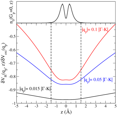
Figure 1: (Color online) The induced potential $\delta V_{\rm{H}}(\mathbf{q}_{p},z)$ in the out-of-plane direction at different values of $|\mathbf{q}_{p}|$, expressed in units of the distance between the $\mathbf{\Gamma}$ and $\mathbf{K}$ points of the Brillouin zone. Calculations were performed for a Fermi level of $\varepsilon_{F}=0.25$ eV, taken from the Dirac point. Details of the numerical calculations can be found in Sec. III.2.1. The typical profile of $n_{0}(\mathbf{G}_{p}=\mathbf{0},z)$ is represented. The equilibrium density was chosen here to have a common reference for all perturbations.

Fig. 1 shows the out-of plane variations of the coarse-grained induced potential $\delta V_{\rm{H}}(\mathbf{q}_{p},z)$ and the equilibrium electronic density $n_{0}(\mathbf{G}_{p}=\mathbf{0},z)$ of a single isolated graphene layer in our ab initio framework. We use three values of $|\mathbf{q}_{p}|$ covering the range of values used in the following section. In that range, Fig. 1 shows negligible variations of the the induced potential over the extent of the electron distribution. The two-dimensional description of the screening properties is thus valid. This range of wavevectors covers a large span of situations where static screening plays a role. For example, in the case of electronic transport we are typically interested in values of $|\mathbf{q}_{p}|$ on the scale of the Fermi wavevector for relatively small doping levels. Thickness effects are negligible in this situation.

IV Results

In this section we present the results of the full DFPT LDA method (Sec. III.2, labelled ”LDA”) and compare them to the analytical solution (Eqs. 32-34, labelled ”Analytical”) for the static dielectric function of doped and neutral graphene. We identify the contributions of temperature, bands, local fields, and exchange-correlation by using different methods. When the analytical derivation presented in Sec. III.1 is used, the Fermi velocity is the only parameter needed to define the Dirac cone band structure. For consistency with the ab initio methods, we use the Fermi velocity obtained in the linear part of the DFT band structure, such that $\hbar v_{F}=5.49$ eV$\cdot$Å. It is well known that electron-electron interactions increase this value by approximately $20\%$ (depending on doping) within the GW approximationAttaccalite et al. (2010). The renormalized value is in good agreement with experiments. This renormalization is ignored here, but should be accounted for when comparing with experiment. Three intermediary methods were used to investigate the differences between the analytical solution and the self-consistent DFPT LDA solution. The first is the semi-numerical method introduced in Sec. III.1. The independent particle susceptibility $\tilde{\chi}^{0}(\mathbf{q}_{p})$ is obtained by numerical integration of Eq. LABEL:eq:exp_chi0, and inserted into Eq. 30. This solution relies on the same approximations as the analytical solution but it can be carried out at a chosen temperature (or energy smearing) as long as the integration grid is adequately fine. The second is labelled ”RPA” and consists in setting the exchange correlation potential to zero within the DFPT method. The third is labelled ”RPA no LF” and consists in evaluating the DFPT independent particle susceptibility and inserting it in Eq. 30. This implies using RPA and neglecting local fields, as well as a strictly 2D treatment, since Eq. 30 was derived in a strictly 2D framework. This method boils down to the evaluation of Eq. 30, within a more complete ab initio model for the band structure. Table 1 summarizes the labels and main characteristics of the various methods used in the following plots.

Table 1: Summary of the various methods used in the plots of Sec. IV. For each method, we report : i) the treatment of electron-electron correlation, LDA refering to the use of the XC potential within LDA, ”$=0$” meaning that the XC potential is set to zero ; ii) wether local fields are included (YES) or neglected (NO) ; and iii) which band structure model was used, the full ab initio band structure or the simpler Dirac cone model for $\pi-\pi^{*}$ bands.

Label	Exchange-Correlation	Local Fields	Bands
LDA	LDA	YES	ab initio
RPA	$=0$	YES	ab initio
RPA no LF	$=0$	NO	ab initio
Analytical	$=0$	NO	Dirac cones

IV.1 Importance of cutting off the Coulomb interactions

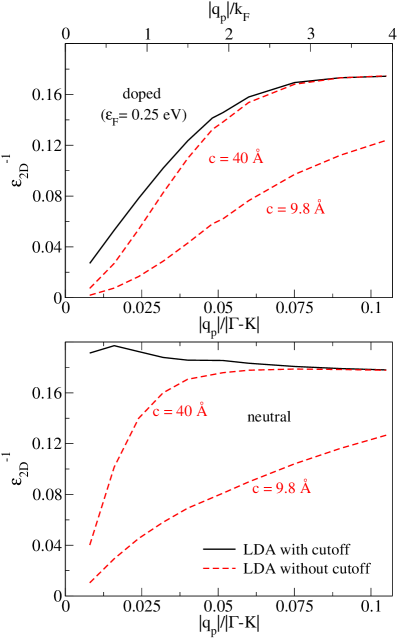
Figure 2: (Color online) DFPT LDA results are plotted with and without cutoff of the Coulomb interactions. The inverse dielectric function, as defined in Eq. 22, is plotted as a function of the adimensional variable $|\mathbf{q}_{p}|/|\mathbf{\Gamma}-\mathbf{K}|$, where $|\mathbf{\Gamma}-\mathbf{K}|\approx 1.7$ Å^-1 is the distance between the $\mathbf{\Gamma}$ and $\mathbf{K}$ points of the Brillouin zone. The calculations were performed for neutral graphene (lower panel) and doped graphene (upper panel) with $\varepsilon_{F}=0.25$ eV, measured with respect to the Dirac point. In the upper panel, we also represent the scale $|\mathbf{q}_{p}|/k_{F}$ where $k_{F}\approx 0.27|\mathbf{\Gamma}-\mathbf{K}|$ refers to the Fermi wavevector in the doped case. Two interlayer distances were used $c\approx 40$ Å and $c\approx 9.8$ Å to convey the dependency of the results (without cutoff) on that parameter. When the Coulomb interaction is cutoff, the results are independent of the interlayer distance $c$. Finally, note that for the neutral case at small wavevectors and with cutoff, the results are quite sensitive to energy smearing/grid effects. In this situation, we used a $140\times 140\times 1$ grid and $0.005$ Ry energy smearing to be as close as room temperature as manageable.

We begin by presenting the DFPT LDA results and pointing out the importance of the Coulomb cutoff in Fig. 2. We plot the inverse dielectric function obtained with the LDA method with and without cutoff. In the latter case, we follow the process of Sec. III.2 but the original 3D Coulomb interaction $v^{3D}_{c}$ is used. Two different interlayer distances are displayed, namely $c\approx 9.8$ Å and $c\approx 40$ Å . It is clear that interlayer interactions play a major role in the screening without cutoff, as a strong dependency on the interlayer distance is shown. For $c\approx 9.8$, the effect of the cutoff is drastic. When the interlayer distance is increased, the results without cutoff slowly approach the results with cutoff. This is also the case in the limit of large wavevector. In general, the results with and without cutoff are similar when the scale on which the induced Hartree potential decreases $1/|\mathbf{q}_{p}|$ is negligible compared to the interlayer distance $c$. However, even using large interlayer distance, the effect of cutting off the Coulomb interactions remains significant. To obtain accurate ab initio results for an isolated layer, it is thus essential to cutoff the Coulomb interactions. To give a clearer picture of the effects of the Coulomb cutoff, we plot the Hartree potential with and without cutoff for two different interlayer distances $c$ in Fig. 3. With cutoff, the Hartree potentials corresponding to the two interlayer distances coincide exactly with each other within the region $[-l_{z};+l_{z}]$, $l_{z}$ being half the smaller interlayer distance here. This confirms that within this region, everything happens as if the layers were isolated. Without cutoff, in contrast, the Hartree potentials are significantly different, stressing the fundamental difference in the response of systems with different interlayer distances.

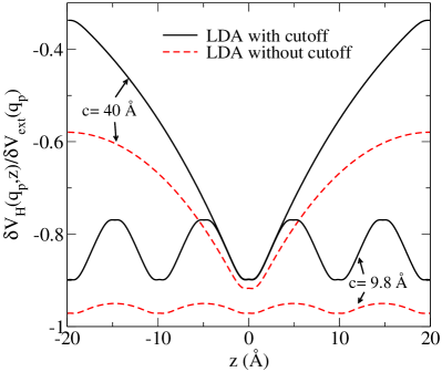
Figure 3: (Color online) The Hartree potentials are plotted in the out-of-plane direction with and without cutoff and for two different interlayer distances $c\approx 40$ Å and $c\approx 9.8$ Å . The calculations were performed for doped graphene with $\varepsilon_{F}=0.25$ eV, at $|\mathbf{q}_{p}|\approx 0.32\ |\mathbf{\Gamma}-\mathbf{K}|\approx 1.2\ k_{F}$.

IV.2 Comparison of analytical and LDA methods: band structure effects

In Fig. 4, we compare the LDA results (with cutoff) to the analytical solution of Eqs. 32-34. The results of the two methods are rather close overall. In doped graphene, the LDA results are in very good agreement ($\approx 3\%$) with the analytical method for $|\mathbf{q}_{p}|\leq 2k_{F}$. A more pronounced discrepancy ($\approx 10\%$) is observed for $|\mathbf{q}_{p}|>2k_{F}$. In the neutral case, a similar $\approx 10\%$ discrepancy occurs for most values of $|\mathbf{q}_{p}|$, but agreement seems to be reached in the small $|\mathbf{q}_{p}|$ limit. For neutral graphene at small wavevectors, smearing plays a significant role. Though not plotted here, the semi-numerical method is equivalent to the analytical solution when performed with an energy smearing corresponding to room temperature. Using the same energy smearing and grid as in DFPT to perform the numerical integration of Eq. LABEL:eq:exp_chi0 showed that smearing effects are negligible except in the small wavevector limit of the neutral case. For DFPT LDA calculations in this regime, we lowered the smearing to $0.005$ Ry and changed the grid accordingly to $140\times 140\times 1$ in Figs. 2 and 4. For this smearing, agreement between LDA and analytical results is reached around $|\mathbf{q}_{p}|\approx 0.025|\mathbf{\Gamma}-\mathbf{K}|$. Although quite low in terms of what is computationally manageable in DFT, this energy smearing is still large compared to the value corresponding to room temperature. At room temperature, we expect that DFPT LDA calculations would show the agreement to be reached for smaller $|\mathbf{q}_{p}|$. In the $0$ temperature limit, it should be reached for $|\mathbf{q}_{p}|\to 0$. Thus, for graphene in general, we can consider that LDA and analytical results significantly differ only for $|\mathbf{q}_{p}|>2k_{F}$, which corresponds to $|\mathbf{q}_{p}|>0$ in the neutral case.

To investigate the origin the $\approx 10\%$ discrepancy above $2k_{F}$, we use the aforementioned ”RPA no LF” method. In Fig. 4, this method gives a smaller inverse dielectric constant than both the LDA ($\approx 8\%$) and analytical ($\approx 16\%$) methods above $2k_{F}$. Comparing the ”RPA no LF” and LDA methods indicates that the combined effect of RPA, neglecting local fields, and a strictly 2D framework is a $\approx 8\%$ decrease of the results. As mentioned before, the band structure model is the only difference between the ”RPA no LF” and analytical methods. This suggests that the effects of using the Dirac cone approximation are more sizable ($\approx 16\%$) but somewhat compensate the other approximations. Overall, we end up with the $\approx 10\%$ discrepancy above $2k_{F}$ between LDA and analytical method. When setting the exchange correlation potential to zero in DFPT, see ”RPA” in Fig.4, the results are only slightly changed. This means that neglecting the local fields in the plane (what is meant by RPA in the derivation of Eq. 30) and out-of-plane (equivalent to making the strictly 2D approximation) have more important effects than exchange-correlation. Although the use of an LDA exchange-correlation potential has negligible consequences for the results presented here, we would like to point out that such potentials are derived in the framework of a three-dimensional electron gas. Consequently, their relevance in a 2D framework is limited and the RPA method might be more reliable than the LDA one.

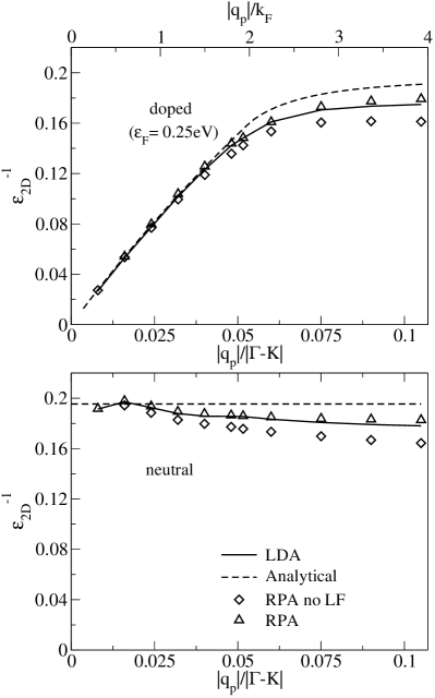
Figure 4: Comparison of the static dielectric function of graphene obtained within the LDA and analytical methods. We use the same axes as in Fig. 2. We also plot the results of the ”RPA” and ”RPA no LF” methods. For this last method applied to neutral graphene, the point with the smallest $|\mathbf{q}_{p}|$ was not converged and is not represented.

A better interpretation of the effects of band structure can be achieved by comparison of the independent particle susceptibility $\tilde{\chi}^{0}$ from the ”RPA no LF” and analytical methods in Fig. 5. In the $|\mathbf{q}_{p}|\leq 2k_{F}$ regime, the screening is dominated by the zeroth-order of $\tilde{\chi}^{0}$, proportional to the density of states. The linear part of the DFT band structure of graphene is well represented by the Dirac cone model. As long as the Fermi level is reasonably small (but finite), the densities of states obtained in DFT and analytically are very close. We then find a very good agreement with the analytical derivation in this regime. In the upper panel of Fig. 5, it is clear that a higher-order (in $|\mathbf{q}_{p}|$ ) term in $\tilde{\chi}^{0}$ from DFPT is responsible for the gradual disagreement with the analytical solution as $|\mathbf{q}_{p}|$ increases. In the neutral case, the zeroth order of $\tilde{\chi}^{0}$ vanishes with the density of state, and $\tilde{\chi}^{0}$ is always dominated by contributions of higher-order terms. For the $|\mathbf{q}_{p}|>2k_{F}$ regime in general, the first-order in $|\mathbf{q}_{p}|$ seems to dominate. The susceptibility $\tilde{\chi}^{0}$ is then ruled by interband processes, some of them going beyond the range of validity of the Dirac cone model.

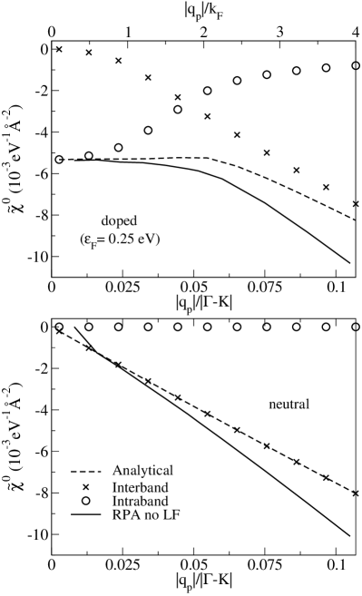
Figure 5: Comparison of the independent electron susceptibility of graphene obtained within the ”RPA no LF” and analytical methods. We use the same axes as in Fig. 2. The contribution of intraband and interband processes to $\tilde{\chi}^{0}$ are represented by circles and crosses, respectively. To calculate those contributions, we used the semi-numerical solution with a small energy smearing ($0.001$ Ry). The analytical and semi-numerical methods are equivalent in that case.

Overall, we find a rather good agreement with the analytical derivation of Refs. Shung, 1986; Gorbar et al., 2002; Ando, 2006; Wunsch et al., 2006; Barlas et al., 2007; Wang and Chakraborty, 2007; Hwang and Das Sarma, 2007. This is in strong contrast with the conclusions of a previous ab-initio studyvan Schilfgaarde and Katsnelson (2011) of the screening of point charges in neutral graphene. Our work differs notably on the use of a Coulomb cutoff, and the treatment of ab initio results to extract the 2D screening properties of a system that is effectively 3D. The authors of Ref. van Schilfgaarde and Katsnelson, 2011 state that they checked the negligibility of the interlayer interactions by looking at the effects of interlayer distance on the bands. Such test is misleading. Indeed, interlayer interactions are negligible on the bands for spacing larger than $\approx 5$ Å. However, as discussed in Sec. II.4, the interlayer interactions affect the calculation of the dielectric response when the wavelength of the perturbation is comparable with the interlayer distance, making the use of a Coulomb cutoff essential. We can also comment on the use of the constant $\kappa_{0}$ in Eq. 7 to include the effects of other bands. Such a constant is not appropriate since it would affect all the orders in $\tilde{\chi}^{0}$, including the zeroth order that is correct. To have an analytic expression quantitatively closer to the DFPT LDA results, one should only renormalize the contribution from the interband processes. Finally, as mentioned before, we used the DFT Fermi velocity in this work. One should keep in mind that within the GW approximation and consistent with experimental results, the Fermi velocity is increased by $20\%$. This yields very similar curves, with a $\approx 16\%$ increase of the value of $\epsilon^{-1}_{2D}$ at large $\mathbf{q}_{p}$, as easily found by plotting the analytical expressions.

V Conclusion

Definitions of the dielectric function depend on the dimensionality. The study of the screening properties of 2D materials first requires precise definitions of the relevant quantities. After setting such a formalism, we review previous analytical derivations of the screening properties of graphene. We highlight the approximations involved in those derivations and propose a DFT-based method to overcome them. The DFPT method with Coulomb cutoff presented here is general and can be applied to study the screening properties of other 2D materials. We showed that cutting off the Coulomb interactions is essential to recover the screening properties of an isolated layer. Our DFPT LDA calculations on graphene lead to an inverse dielectric function that is very close to the analytical form of Refs. Shung, 1986; Gorbar et al., 2002; Ando, 2006; Wunsch et al., 2006; Barlas et al., 2007; Wang and Chakraborty, 2007; Hwang and Das Sarma, 2007 for $|\mathbf{q}_{p}|\leq 2k_{F}$, and smaller by $\approx 10\%$ for $|\mathbf{q}_{p}|>2k_{F}$. Overall, the Dirac cone model in a strictly 2D framework, in the zero temperature limit, using RPA and neglecting local fields leads to a quite accurate and simple analytical expression for the static dielectric function of graphene. Smearing effects are negligible at room temperature and exchange-correlation effects within LDA are also quite small. Neglecting the local-fields leads to a $\approx 8\%$ underestimation of the inverse dielectric function above $2k_{F}$. The largest error comes from the Dirac cone model for the band structure. This model remains an excellent approximation in the $|\mathbf{q}_{p}|\leq 2k_{F}$ regime, as long as the Fermi level lies in the region where the bands are linear. In the $|\mathbf{q}_{p}|>2k_{F}$ regime, however, the Dirac cone model leads to a $\approx 16\%$ overestimation of the inverse dielectric function due to the contribution of interband processes probing states beyond the Dirac cones. This overestimation compensates the local fields effects and the analytical model ends up overestimating the DFPT LDA inverse dielectric function by $\approx 10\%$ above $2k_{F}$.