Higher-order root distillers

Abstract

Recursive maps of high order of convergence $m$ (say $m=2^{10}$ or $m=2^{20}$) induce certain monotone step functions from which one can filter relevant information needed to globally separate and compute the real roots of a function on a given interval $[a,b]$. The process is here called a root distiller. A suitable root distiller has a powerful preconditioning effect enabling the computation, on the whole interval, of accurate roots of an high degree polynomial. Taking as model high-degree inexact Chebyshev polynomials and using the Mathematica system, worked numerical examples are given detailing our distiller algorithm.

1 Introduction

By a higher-order root distiller we mean an algorithm to compute, simultaneously, all (or almost all) the real roots of a polynomial $f$ of (high) degree $d$, in a given interval $[a,b]$. The algorithm relies on a single application, on the interval, of a map $g$ of (very) high order of convergence $m$ (for instance $m=2^{10}=1024$ or $m=2^{20}=1\,048\,576$). The approach may be seen as a modern computational perspective of the global Lagrange’s ideal [1].

Once defined such a higher-order map $g$, the roots of the function $f$ in the interval are obtained from a table $\mathcal{L}=\left\{(x_{1},y_{1}),(x_{2},y_{2}),\ldots,(x_{N},y_{N})\right\}$, where $y_{i}=g(x_{i})$, and $x_{i}$ belong to an uniform grid (of $N+1$ nodes) of width $h$, defined on $[a,b]$. For suitable choices of $h$ and $k$ (the parameter $k$ controls the order of $g$), the map $g$ induces an invariant monotone step function leading to certain subsets of $\mathcal{L}$, say $S_{1},S_{2},\text{...},S_{i},\text{...},S_{r}$. These subsets will be called ‘platforms’ (see Section 3) and have the property that the second component of the points $(x,y)_{i}$ on the platform $S_{i}$ are equal to (or close to) the i-th root of the polynomial.
A graphical inspection of the list $\mathcal{L}$ may be useful not only to observe the distribution of the roots in $[a,b]$ but also to suggest good choices for the two parameters controlling the algorithm, which are the mesh width $h$ and the index $k$, the latter related to the order of convergence $m$ of the map $g$ ($m=2^{k+1}$ in the case of simple roots).

Although in this work we only deal with roots of polynomials, the same procedure can be adapted to non-algebraic equations $f(x)=0$ having at least one root in a given interval, or with the case of multiple roots or even to functions in $\mathbb{R}^{n}$ [2].

In finite arithmetic, one of the main feature of our distiller process is that, by construction, the values $y_{i}$ are generally quite immune to rounding error propagation. Therefore a roots’s distiller can be seen as a powerful pre-conditioning instrument, in particular for polynomials whose coefficients are numeric. The referred immunity to rounding error propagation is closely related to the fact that a map of higher-order of convergence leads necessarily to a stationary ‘monotone machine step function’ — if the recursive process which generates the map $g$ is taken appropriately, that is, for $k$ sufficiently large. Details on the monotone machine step functions are further explained in sections 2 and 3.

Thanks to the super-attracting property of a map of a high order of convergence, each tread (or ‘platform’) of the monotone machine step function – corresponding to the theoretical subsets $S_{i}$ referred above– contains several machine accurate values $y_{i}$ which are close approximations of the zeros of the given function $f$. In general, all the necessary information in order to approximate the zeros of a given map with a prescribed accuracy is contained in these treads.

Our root distiller is constructed in order to overcome some common numerical issues appearing in the computation of zeros of a given function and in particular of roots of polynomials of high degree. It is well known the inherent ill conditioning of the computation of polynomial roots. For instance Mathematica commands for approximating roots of polynomials of high degree may produce useless numerical results when low-precision finite arithmetic is used. On the other hand, dealing with exact polynomials of high degree $d$, say $d\geq 100$, prevents us from using exact arithmetic due to CPU excessive cost.
To be more precise, suppose that a numeric expression for the (first kind) Chebyshev polynomial of degree 40 is defined by the command N[ChebyshevT[40, $x],8]$, where the coefficients are deliberately forced to have 8-digits precision. The commands Solve, Reduce, and Roots produce useless numerical results (cf. paragraph 1.1) since the computed roots are heavily contaminated by rounding error (even though the degree $d=40$ of such polynomial is moderate). Our root distiller deals efficiently not only with this case but it also produces accurate answers, for instance with a $500$-degree Chebyshev polynomial.

In Section 2 we detail the construction of a specific map $g$. For that, it is given a positive integer $prec$ and two parameters $h$ and $k$. The parameter $k$ controls the order of the map $g$ to be constructed, $h$ is the mesh size and $prec$ fixes the precision to be used in the computations of the images $y_{i}=g(x_{i})$ in the list $\mathcal{L}$.

In Section 3 it is illustrated how a map $g$ of high order of convergence leads to a monotone step function which contains the relevant information to be distilled. We chose as basic model a 4-degree Chebyshev polynomial of the first kind with $prec=8$ and the parameters $h=0.1$ and $k=3$. The respective map $g$ has order of convergence 16 and the absolute error of computed roots is of order $10^{-8}$, meaning that the accuracy used on $\mathcal{L}$ is preserved.

Mathematica code is presented in sections 2 and 4, including the process used for filtering the relevant values in the respective list $\mathcal{L}$ (other filtering possibilities may also be considered).

Numerical examples have shown the efficiency of the proposed distillers. In particular, we construct here a distiller for the computation of the positive roots of the Chebyshev polynomial of degree 500, defined in $[-1,1]$, with precision forced to be $prec=5000$ and parameters $h=0.00025$ and $k=20$ (and so the respective map $g$ has order of convergence $m=2^{21}=2\,097\,152$). The computed roots have 5000-correct digits.

An automatic choice of appropriate parameters $h$ and $k$ in order to achieve a preassigned tolerance error can be done, but this is out of the scope of the present work.

1.1 Motivation: a low precision Chebyshev polynomial

Setting the precision $prec=8$, we obtain the following Mathematica expression for the Chebyshev’s polynomial of degree 40, $N[ChebyshevT[40\,,\,x],\,prec]$:

$$\begin{array}[]{l}1.0000000-800.00000x^{2}+106400.00x^{4}-5.6179200\times 10^{6}x^{6}+\\ +1.5690048\times 10^{8}x^{8}-2.6777682\times 10^{9}x^{10}+3.0429184\times 10^{10}x^{12}-\\ -2.4343347\times 10^{11}x^{14}+1.4240858\times 10^{12}x^{16}-6.2548083\times 10^{12}x^{18}+\\ +2.1002988\times 10^{13}x^{20}-5.4553215\times 10^{13}x^{22}+1.1029237\times 10^{14}x^{24}-\\ -1.7375290\times 10^{14}x^{26}+2.1236466\times 10^{14}x^{28}-1.9918340\times 10^{14}x^{30}+\\ +1.4055280\times 10^{14}x^{32}-7.2155451\times 10^{13}x^{34}+2.5426206\times 10^{13}x^{36}-\\ -5.4975581\times 10^{12}x^{38}+5.4975581\times 10^{11}x^{40}.\end{array}$$

The Mathematica commands Solve, Reduce and Roots produce, respectively, the following useless output:

Of course the commands NSolve and NRoots also give useless values.

We aim to obtain ‘machine’  acceptable answers, that is to compute the real roots of the 40-degree Chebyshev polynomial in the interval $[a,b]=[-1,1]$, which are simple and distinct, with an accuracy close to that of the data (recall that 8-digits precision has been assigned to the polynomial coefficients).

The algorithm which we call ‘root distiller’ is described in what follows, and shows to be able to accomplish such a desideratum. The code can easily be included in a single function in order to produce the referred machine point list $\mathcal{L}$, once predefined the function f, the bounds of the interval, the preassigned precision $prec$ and the mesh size $h$. After a convenient filtration of the data in $\mathcal{L}$, the respective output should be considered global in the sense that it is able to (simultaneously) produce accurate approximations of the roots in the interval, as well as realistic error estimates to each of them (see Section 4).

2 Higher-order educated maps and monotone step functions

In a global approach to roots’s computation by means of a smooth high order of convergence map $g:[a,b]\subset\mathbb{R}\longrightarrow\mathbb{R}$, many of the domain points are irrelevant, in the sense that their image under $g$ might not be a number or is repealed from a fixed point of $g$. In fact any map of order of convergence greater than one enjoys such a repealing/attracting property – like in the well known cases of the Newton’s or secant methods for approximation of simple roots. So, once defined a map $g$ of sufficiently high order of convergence, the points which are not a number, nor in the interval $[a,b]$, neither attracted to a fixed point will be ignored. This is the reason why we then will call $g$ an ‘educated’  higher-order map.

In general, the recursive maps to be considered have order $m$ of convergence which can go up to $m=2^{10}=1024$, or greater. The recursive process used to define the map makes possible to obtain a monotone step function defined in the interval $[a,b]$. From this step function one extracts the relevant computed $g$-images through a filtering process in order to obtain as output most, or all, the roots of the equation $f(x)=0$. In particular, our distillers will allow us to compute the roots of a Chebyshev’s polynomial of high degree, a task not feasible by the exact methods provided by the Mathematica system (version 10.02.0 running on a Mac OS X personal computer has been used in this work), unless the interval is small and the working precision high.

2.1 Recursive construction of the higher-order map g

We now explain the recursive construction of a map $g$ of high order of convergence by taking as a seed the Newton’s map. The map $g$ is the $k$-fold composition of this seed and has order of convergent $m=2^{k+1}$. The construction of $g$ goes through and ‘education’ process aiming to obtain a map satisfying a fixed point theorem in the interval [a,b]. More precisely, $g$ is constructed in order to satisfy the following properties:

• $g([a,b])\subseteq[a,b]$ .

• $|g(x)-x|\leqq(b-a)$, for all $x$ for which  NumericQ[g(x)] is True .

• The points $x\in[a,b]$ not satisfying (i) and (ii) are ignored (a Null is assigned to $g(x)$) .

For $k$ sufficiently high, the educated map $g$ will act on $[a,b]$ as a kind of a ’magnet’  having both good theoretical and computational properties. This ‘magnetic’ property is better perceived by inspecting a plot of the respective induced monotone step function.

It can be proved that for a fixed mesh size $h$, an educated map induces an invariant (or stationary) monotone step function, whenever the folding parameter $k$ is sufficiently large. This invariant step function will be called the machine step function associated to a map $g=g[h,k]$.

Choosing suitable values for $k$, the second component of points on the treads or ‘platforms’  of the associated step function contain (by construction) accurate approximations of the roots of $f(x)=0$. Moreover, the platforms of such step function are automatically sorted in increasing order of their heights, defining so a monotone step function in the interval $[a,b]$. The later filtering process of the data of this step function will hopely solve the referred global Lagrangian root’s problem.

In the following illustrative example an uniform mesh of points, of width $h$, is defined on the domain range $[a,b]$. The ListPlot command is used in order to observe the behaviour of an higher-order educated map $g$ on the referred mesh.

Although in this work the seed used in the recursive process is the Newton’s map, any other method of order of convergence greater than one could be used. For instance, the secant method, of order $(1+\sqrt{5})/2$, and Ostrowsky’s methods, of orders $\geq 3$, are other obvious options.

2.2 The map g from the Newton’s seed

Fixing a precision $prec$, assume that the numeric expression for a given function $f$ is in memory as well as the bounds $a$ and $b$ of the interval where the roots of $f(x)=0$ are required. Given the (folding) parameter $k$, the following code defines a general recursive function g[x,prec] using Newton’s map as seed (see below functions newt[0,x,prec] and its recursive version newt[k,x,prec]). The map $g$, of order of convergence $m=2^{k+1}$, is given below as the function named g[x,prec].
Note that when $y$=g[x,prec] is a number, the assigned precision to $y$ is forced to be the same as the precision of $x$. This prevents the Mathematica system to correct the output of each calculation of $y$ in the case it occurs of a loss of significant digits. The code for the function g[x,prec] follows.

3 An illustration with a low precision 4-degree Chebyshev polynomial

As an illustration of the occurrence of a monotone step function induced by the map $g$, let us consider a 4-degree Chebyshev polynomial in the interval $[a,b]=[-1,1]$, and define an uniformly spaced mesh of width $h=0.1$ (that is 21 equally spaced nodes). We apply the above g[x,prec] code, with assigned parameters $prec=8$ and $k=3$, that is, in this case the map $g$ has order of convergence $m=2^{k+1}=16$.

In Figure 1 it is displayed the plot of the respective point list $\mathcal{L}$ and the computed values $g[x,prec]$. This figure is self-explanatory: there are 4 roots corresponding to the 4 platforms in the displayed graphic; an increasing step function is suggested by the dotted broken line. Each of the four observed platforms is formed by a set of points and from this set of pairs $(x,y)$ we filter the value $y$ of the pair which has the second component closer to the first. The value of $y$ filtered this way is an approximation of a polynomial’s root. In this example, the 4 points filtered are displayed in the last column of the table. These 4 values are 8-digit accurate roots of the Chebyshev polynomial of degree 4.

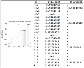
Figure 1: A step function associated to a 8-digits precision, 3-fold map $g$, applied to a 4-degreed Chebyshev polynomial.

Looking at the second column of the table in Figure 1, it is clear the super-attracting property of the ‘magnet’  $g$: all the numeric points in each platform have the second component very close to the respective exact fixed point of the map $g$. Repetting the computations for $k=4$, the corresponding table is identical to the one in Figure 1, except the image of $x=-0.8$, which is $-0.92387953$. This means that the respective map $g$, now of order $2^{k+1}=32$, is invariant and so the former computed roots have indeed 8 correct digits. Saying it in other words – the 4 computed values are ‘machine’  fixed points for this map (see the last column in Figure 1).

4 Distilling Chebyshev polynomials of high degree

For a given precision $prec$ and appropriate parameters $h$ and $k$, we developed a simple Mathematica code which will be tested in order to approximate the roots of high degree Chebyshev polynomials. A realistic estimative of the error of each computed root is also easily obtained. In fact, if $g$ has order of convergence $m>1$ and $y=g(x)$ is a value close to a fixed point $\alpha$, the error of $y$ satisfies $\alpha-y\simeq g(y)-y$.

Concerning our polynomial models, since the roots become closer when we increase the degree of the Chebyshev’s polynomial, the value of the mesh size $h$ and the parameter precision $prec$ need to be adjusted accordingly. Our aim is to obtain a highly accurate bound for the positive roots of a 500-degree Chebyshev polynomial of the first kind.

4.1 Example: a 500-degree Chebyshev polynomial

A 500-degree Chebyshev’s polynomial is highly oscillating and so its roots are very close. Therefore, it is necessary to set a sufficiently large value of the precision $prec$, and choose a convenient mesh size $h$ in order to obtain the required numerical results. We consider now the interval to be $[0,1]$.

In order to observe the platforms of our distiller, we display the plots of the educated maps $g$ for some values of the parameter $k$ and of $prec$ as a guide for the choice of the right values of these parameters. The next figure compares the graphics of the function g[x, 100], respectively for $k=0$ and $k=10$ (the mesh size in the plot is not uniform since it is automatically generated by function Plot in the interval $[a,b]$).

It is clear from Figure 2 that a $100$-digits precision is not enough to obtain the roots localised on the right-half domain, while one can expect a good separation of roots in the interval by setting $prec=5000$, as suggested by Figure 3.

Figure 2: For $prec=100$ and a mesh automatically generated by $Plot$, only the roots localised on the left half-domain are detected.

Figure 3: Increasing $prec$ to $prec=5000$ and for $k=10$-folding, the roots on $[0,1]$ of the 500-degree Chebyshev’s polynomial are detected.

An advantage of choosing an higher order of convergence map $g$ will become more apparent if we restrict the interval to $[0.9,1.0]$, which contains the desired greatest root of the polynomial. We proceed with the computation of a $5000$ correct digits bound for the positive roots of the polynomial by using a distiller whose folding parameter is $k=20$ (the respective educated map has order $m=2^{21}=2\,097\,152$). We note that this time the graphics are quickly produced since we use ListPlot instead of Plot and therefore the respective mesh has now much less points than in the usage of Plot.

4.2 The filtering stage

Efficient Mathematica commands for manipulating lists, such as $Cases$, $Parti\-tion$ and $Union$, are particularly useful in the filtering stage of the distiller algorithm.
Assume that all the numeric points in $\mathcal{L}$ have been assigned to a list named $data$. The first step in the filtration deals with the choice of points $(x,y)$ sufficiently close to the bisector line, that is to the line $y=x$. We test the condition say, $\left|y-x\right|^{2}<0.1$, on the $data$ list, and assign the captured points to a sublist named data1, as follows

data1 = Cases[data, x, y; Abs$[y-x]^{2}<0.1$ ]; (* distille close to bissector *)

The points in data1 belonging to a certain platform (that is to a ‘horizontal’  segment crossing the bisector line) are good candidates for an approximation of the root. The next sublist, named $data2$, keeps the interesting points. These points are chosen in order to satisfy the condition $(y_{1}-x_{1})(y_{2}-x_{2})<0$, which assures that at least a machine fixed point exists in the interval denoted by $[x_{1},x_{2}]$:

data2=
Cases[Partition[data1,2,1],{{x1_,y1_},{x2_,y2_} }/;(y1-x1)*(y2-x2)<0 ];

For a given tolerance, say $tol=10^{-\text{prec}}$, we are interested in filtering the points in the list $data2$ whose second component $y$ differ from an amount greater than $tol$. Using the command Union, we project the platform ignoring machine-duplicate-numbers, obtaining a sublist named $union$,

union = Union[Map[Last, Flatten[data2, 1] ]];

The final step in the filtering process checks for the accuracy of the former captured points. First, one filters the values $y$ in the list $union$ for which $f(y)$ is not greater than say $10^{-5000}$. The result is assigned to a sublist called finalA. Second, one filters the values $y$ in the list $finalA$, whose estimated absolute error is less than a tolerance, say $tol=10^{-5000}$ . An error bound for each machine root is also computed. The respective code follows.

finalA = Cases[union, y_ /; f[y] < $10^{-5000}$];

mapf = Map[$\{$#, g[#, prec] - #$\}$ &, finalA]; (* roots and error *)

tol = $10^{-100}$;

final = Cases[mapf,$\{$x_, error_$\}$/;Abs[error]< tol]; (* error bound *)

Assembling the above filtering stage and the one given at paragraph 2.2, a general function is easily obtainable for the whole distiller algorithm.

4.3 A $5000$-correct digits approximation for the bound of the positive roots

We now apply our distiller to compute a bound for the positive roots of the 500-degree Chebyshev polynomial in $[0.99,1.0]$, with an error not exceeding $10^{-5000}$. Since a bound for the positive roots of the polynomial is required, only the greatest computed root in the interval will be displayed as well as its estimated error.

In Figure 4 the ListPlot of the map $g$ is shown, where here $g$ is the Newton’s educated method ($k=0$), the precision is $prec=5000$, and the mesh size $h=0.00025$. After filtration an empty list is obtained, meaning that this map is useless under the previously described filtering criteria. So a more powerful ‘magnet’  should be used, that is, one needs to increase the order of convergence of $g$ by taking a greater value of the folding parameter $k$.

Figure 4: After filtration no points have been captured using the Newton’s seed.

Increasing to $k=10$, the respective 2048-order map $g$ (Figure 5 left) enable us to filter relevant points (see Figure 5 right) from which high precision roots can be distilled.

Figure 5: For a $10$-fold map the points in the list $data2$ of the respective ‘machine’  step function are shown on the right.

For $h=0.0025$ and $k=20$ (Figure 6), the complete filtration process leads to 20 fixed points, which are the machine roots of the $500$-degree Chebyshev polynomial, in the interval $[0.99,1.00]$, for the considered distiller.

Figure 6: Points captured by a 20-fold $g$ map.

Denoting by $\alpha$ the last computed root, a 5000 correct digits bound is obtained. Respectively the first 100 and the last 100 digits of $\alpha$ are displayed below, as well as its estimated error.

Note that a Mathematica instruction such as

$$x\,/.\,Solve[\{f[x]==0,0.99\leq x\leq 1.0\},x]\}$$

does not produce an answer within an acceptable CPU running time.

Of course, the classical formula giving the zeros of a d-degree Chebyshev polynomial, $\alpha_{j}=\cos\left(\frac{(2j+1)\pi}{2d}\right)$, for $j=0,...(d-1)$, can be used in order to confirm the above computed value of $\alpha$.

References

- [1] Lagrange, J. L.,Traité de la résolution des équations numériques de tous les degrés. Paris, 1808 ib.1826. (Available at http : // dx.doi.org/10.3931/e - rara - 4825).
-
[2]
Mário M. Graça, Recursive families of higher order iterative maps,
arXiv:1405.4492 [math.NA], 18 May 2014.