HOW BAD/GOOD ARE THE EXTERNAL FORWARD SHOCK AFTERGLOW MODELS OF GAMMA-RAY BURSTS?

Abstract

The external forward shock models have been the standard paradigm to interpret the broad-band afterglow data of gamma-ray bursts (GRBs). One prediction of the models is that some afterglow temporal breaks at different energy bands should be achromatic, namely, the break times should be the same in different frequencies. Multi-wavelength observations in the Swift era have revealed chromatic afterglow behaviors at least in some GRBs, casting doubts on the external forward shock origin of GRB afterglows. In this paper, using a large sample of GRBs with both X-ray and optical afterglow data, we perform a systematic study to address the question: how bad/good are the external forward shock models? Our sample includes 85 GRBs up to March 2014 with well-monitored X-ray and optical lightcurves. Based on how well the data abide by the external forward shock models, we categorize them into five grades and three samples. The first two grades (Grade I and II) include 45/85 GRBs. They show evidence of, or are consistent with having, an achromatic break. The temporal/spectral behaviors in each afterglow segment are consistent with the predictions (the “closure relations”) of the forward shock models. These GRBs are included in the Gold sample. The next two grades (Grade III and IV) include 37/85 GRBs. They are also consistent with having an achromatic break, even though one or more afterglow segments do not comply with the closure relations. These GRBs are included in the Silver sample. Finally, Grade V (3/85) shows direct evidence of chromatic behaviors, suggesting that the external shock models are inconsistent with the data. These are included in the Bad sample. We further perform statistical analyses of various observational properties (temporal index $\alpha$, spectral index $\beta$, break time $t_{b}$) and model parameters (energy injection index $q$, electron spectral index $p$, jet opening angle $\theta_{j}$, radiative efficiency $\eta_{\gamma}$, etc) of the GRBs in the Gold Sample, and derive constraints on the magnetization parameter $\epsilon_{B}$ in the forward shock. Overall, we conclude that the simplest external forward shock models can account for the multi-wavelength afterglow data of at least half of the GRBs. When more advanced modeling (e.g., long-lasting reverse shock, structured jets, arbitrary circumburst medium density profile) is invoked, up to $>90\%$ of the afterglows may be interpreted within the framework of the external shock models.

1 Introduction

Gamma-ray bursts (GRBs) are the most luminous explosions in the universe. They signify the birth of a stellar-mass black hole or a rapidly rotating magnetized neutron star during core collapses of massive stars or mergers of compact objects (Kumar & Zhang, 2015, for a recent review).

Multi-wavelength GRB afterglows were predicted (Mészáros & Rees, 1997) before their first discoveries (Costa et al., 1997; van Paradijs et al., 1997; Frail et al., 1997). This was based on a generic external forward shock model. Regardless of the physical nature of progenitor and central engine, a relativistic jet is launched, which is decelerated by a circumburst medium by a pair of external (forward and reverse) shocks. The reverse shock is likely short-lived. The forward shock, on the other hand, continues to plough into the medium as the jet is decelerated. Synchrotron radiation of electrons accelerated from the external forward shock powers broad-band electromagnetic radiation with a decreasing amplitude. This is the broad-band afterglow of GRBs (Mészáros & Rees, 1997; Sari et al., 1998; Mészáros et al., 1998; Rhoads, 1999; Sari et al., 1999; Chevalier & Li, 2000).

Before 2004, the observations of the broad band late time afterglow emission of GRBs generally show broken power-law lightcurves and instantaneous spectra. Detailed studies (e.g., Wijers et al., 1997; Waxman, 1997; Wijers & Galama, 1999; Harrison et al., 1999; Huang et al., 1999, 2000; Panaitescu & Kumar, 2001, 2002; Yost et al., 2003; Wu et al., 2004) suggested that these late-time data are generally consistent with the predictions of the external forward shock models.

The launch of the Swift satellite in 2004 (Gehrels et al., 2004) allowed systematic observations of the multi-wavelength GRB afterglow at early epochs. These data, especially the early X-ray afterglow data, presented surprises to modelers. The overall X-ray lightcurves include five distinct temporal components (Zhang et al., 2006): I: an early time steep decay phase connected to the prompt emission (Tagliaferri et al., 2005; Barthelmy et al., 2005; Zhang et al., 2007c); II: a shallow decay (or plateau) phase, which may signify continuous energy injection of energy into the blastwave (Zhang et al., 2006; Nousek et al., 2006; Liang et al., 2007); III: a normal decay phase consistent with the forward shock emission of a constant-energy fireball; IV: a late steep decay phase likely due to a jet break origin (e.g., Liang et al., 2008; Racusin et al., 2009); and V: erratic X-ray flares, likely powered by late central engine activities (Ioka et al., 2005; Burrows et al., 2005; Fan & Wei, 2005; Zhang et al., 2006; Liang et al., 2006; Lazzati & Perna, 2007; Chincarini et al., 2007; Maxham & Zhang, 2009; Margutti et al., 2010). The components I and V are are believed to be of an internal origin (in contrast to the external shock origin). The other three components (II, III and IV) may be interpreted within the framework of the external shock models.

The optical afterglow light curves also show interesting temporal behaviors (Liang et al., 2006; Nardini et al., 2006; Kann et al., 2006, 2010, 2011; Panaitescu & Vestrand, 2008, 2011; Li et al., 2012; Liang et al., 2013; Wang et al., 2013; Yi et al., 2013). In the similar spirit as Zhang et al. (2006), Li et al. (2012) attempted to summarize a “synthetic” light curveof optical emission. They found more components with distinct physical origins: Ia: prompt optical flares; Ib: an early optical flare of an external reverse shock origin; II: an early shallow-decay segment; III: the standard afterglow component (the normal decay component, sometimes with an early onset hump); IV: the post-jet-break phase; V: late optical flares; VI: late rebrightening humps; and VII: late supernova (SN) bumps. The components II, III and IV can find their counterparts in the canonical X-ray light curve (components II, III, and IV in Zhang et al. 2006). Some flares in the optical band have counterparts in X-rays, but some others do not (Swenson et al., 2013). Some components (e.g., the reverse shock component Ib and the supernova component VII) are unique for the optical band only.

There are two types of temporal breaks in the external shock models. One type corresponds to the crossing of a characteristc frequency in the observational band (Sari et al., 1998). Such spectrally-related breaks occur at different epochs in different energy bands, and therefore are chromatic. A testable feature of such a break is that the spectral indices before and after the temporal break should be distinctly different. The second type of breaks are related to the hydrodynamic or geometric properties of the system. Since both effects affect the global behavior of the blastwave, these breaks should be achromatic, i.e. the temporal breaks in different energy bands should occur around the same observational time.

Most observed breaks in the GRB lightcurves are likely of a hydrodynamic or geometric origin. Observationally, essentially all the temporal breaks observed in the X-ray lightcurves are consistent with having no spectral changes across the break times (Liang et al., 2007, 2008). Theoretically, the spectral breaks, especially the cooling break, are predicted to be very smooth, and are barely observable from the data (Uhm & Zhang 2014a, see also Granot & Sari 2002; van Eerten & Wijers 2009). As a result, one expects that the temporal breaks seen by Swift should be strictly achromatic based on the external forward shock models.

Broad-band afterglow data of GRBs are rapidly accumulating. Shortly after Swift detected early X-ray afterglow lightcurves of GRBs, some authors noticed that the basic requirement of achromaticity of GRB afterglows is violated at least in some GRBs (e.g., Panaitescu et al., 2006; Fan & Piran, 2006; Huang et al., 2007; Liang et al., 2007, 2008). In particular, while a significant break is seen in the X-ray lightcurves of some GRBs, the optical lightcurve does not show evidence of a break at the corresponding time (e.g., Troja et al., 2007; Molinari et al., 2007). Such a puzzling effect led theorists to suggest various non-forward-shock models of the X-ray afterglow: the long-lasting reverse shock model (Genet et al., 2007; Uhm & Beloborodov, 2007), the dust scattering model (Shao & Dai 2007), and the long-lasting central engine model (Ghisellini et al., 2007; Kumar et al., 2008a, b).

Indeed, if most GRB afterglows are chromatic, one must throw away the standard forward shock paradigm, and probably attribute other factors, in partular, the long-lasting central engine, to account for the X-ray afterglow. This would have profound implications for our understanding of the GRB central engine and emission physics. Yet, there seem to exist some GRBs (e.g., the latest bright GRB 130427A) whose multi-wavelength data are consistent with the simplest forward shock afterglow model (e.g., Maselli et al., 2014; Perley et al., 2014).

It is therefore natural to ask the following question: in general how bad or how good are the external forward shock models in interpreting the GRB afterglow data?

This paper aims at addressing this question through a systematic data analysis and theoretical modeling of a large sample of multi-wavelength afterglows. We study a sample of 85 Swift GRBs up to March 2014, which all have high-quality X-ray and optical light curve data to allow us to study the compliance of the data to the external forward shock models. The sample selection and data analyses are described in §2. The theoretical external forward shock model, in particular, the so-called closure relations are presented in §3. In §4, we grade the afterglows based on how well they abide by the forward shock models, and categorize them into five grades and three samples. A statistical analysis of various observational and theoretical parameters for the Gold sample is presented in §5. Our results are summarized in §6 with some discussion. We notice that Li et al. (2015) recently carried out a similar analysis, with the focus on the consistency of the data with afterglow models in individual temporal segments of X-ray and optical lightcurves, without analyzing the global achromatic/chromatic behaviors of the afterglows.

Throughout the paper, the subscripts “O” and “X” denote the optical and X-ray band, respectively, and the subsripts “1” and “2” denote the pre- and post-break segments, respectively. In addition, two spectral regimes are defined: “I” for $\nu>{\rm max}(\nu_{m},\nu_{c})$, and “II” for $\nu_{m}<\nu<\nu_{c}$, where $\nu_{m}$ and $\nu_{c}$ are the minimum injection frequency and cooling frequency for synchrotron radiation, respectively.

2 Sample and Data

We systematically investigate all the Swift GRBs that have X-ray and optical afterglow data, over a span of almost 10 years from the launch of Swift to March 2014. A sample of $\sim$260 optical light curves are compiled from published papers or GCN Circulars, and a sample of $\sim$900 X-ray light curves are obtained from the Swift XRT data archive. Well-sampled light curves in both X-ray and optical bands are available for 99 GRBs. Fifteen GRBs do not have well constrained spectral indices either in optical or in X-ray bands to allow us to perform some theoretical constraints (see details below). Fourteen of them are removed from the sample. GRB 070420 is the only GRB without adequate spectral information that is included in our sample. This is because it has a clear chromatic feature, which allows us to group it into the Bad sample even if the spectral information is not available (see details in §4.2). The remaining 84 GRBs are included in our final sample, whose information is presented in Table 1. For the optical data, the correction due to Galactic extinction is taken into account using the reddening map presented by Schlegel et al. (1998). Due to large uncertainties, we do not make corrections to the extinction in the GRB host galaxies.

In order to quantify the rich temporal features of GRB lightcurves, we fit the lightcurves with a model of multiple components. The basic component of our model is either a single power-law (SPL) function

$$F_{1}=F_{01}t^{-\alpha}$$ (1)

or a smooth broken power-law (BPL) function

$$F_{2}=F_{02}\left[\left(\frac{t}{t_{\rm b}}\right)^{\alpha_{1}\omega}+\left(\frac{t}{t_{\rm b}}\right)^{\alpha_{2}\omega}\right]^{-1/\omega},$$ (2)

where $\alpha$, $\alpha_{1}$, $\alpha_{2}$ are the temporal slopes, $t_{\rm b}$ is the break time, and $\omega$ measures the sharpness of the break. In some afterglow models, a double broken power-law light curve is expected. For example, it is theoretically expected that the afterglow light curve may have a shallow segment early on due to energy injection, then transits to a normal decay segment when energy injection is over, and finally steepens due to a jet break (e.g., in the canonical X-ray afterglow lightcurve, Zhang et al. 2006). We therefore also consider a smooth triple-power-law (TPL) function to fit some lightcurves. In these cases, we extend equation (2) (with $t_{b}$ defined as $t_{b,1}$) to the following function (Liang et al., 2008)

$$F_{3}=(F_{2}^{-\omega_{2}}+F_{4}^{-\omega_{2}})^{-1/\omega_{2}}$$ (3)

where $\omega_{2}$ is the sharpness factor of the second break at $t_{b,2}$, and

$$F_{4}=F_{2}(t_{\rm b,2})\left(\frac{t}{t_{b,2}}\right)^{-\alpha_{3}}.$$ (4)

We perform best fits to the data using a subroutine called MPFIT. The sharpness parameter $\omega$ is usually adopted as 3 or 1 in our fitting. The parameter $t_{b}$ is not significantly affected by the choice of $\omega$, but the pre- and post-break slopes (i.e. $\alpha_{1}$ and $\alpha_{2}$) somewhat depend on the value of $\omega$ (Liang et al., 2007). The larger the value of $\omega$, the sharper the break. The breaks in most X-ray and optical light curves at later times (e.g. the energy injection breaks and the jet breaks) can be well fit with $\omega=3$, which is consistent with the fitting results using other empirical models (e.g. Willingale et al., 2007). Some very smooth breaks (e.g., the onset breaks in the early optical lightcurve curves) require $\omega$ being around 1 Liang et al. (2007); Li et al. (2012), and we adopt this value when it is needed.

One focus of our analysis is to study the “chromaticity” of the lightcurves in the X-ray and optical bands. In principle there are two approaches to do this. The first approach is to blindly search for $t_{b}$ using the best fits to the optical and X-ray data, respectively, and compare how different the two $t_{b}$ values are. Such an approach usually gives different break times in the two bands (Liang et al., 2007, 2008; Li et al., 2012, 2015). The second approach is to start with the achromatic assumption and investigate how bad the data violate such an assumption. By doing so, we reduce one free parameter, and impose a same $t_{b}$ in both bands in the model. We believe that this second approach is more reasonable to address the question “how bad the external forward shock models are”, so we adopt the second approach with the assist of the first approach. The detailed procedure of our light curve fitting is as follows:

• For each GRB, we first fit the optical and X-ray afterglow light curves separately, and get the respective fitting parameters, such as $t_{\rm O,b}$, $t_{\rm X,b}$, and the $\omega$ values of each break). A minimum number of components (SPL, BPL, or TPL) are introduced based on eye inspection of the global features in the lightcurve. If the reduced $\chi^{2}$ is much larger than 1, we continue to add more components and re-do the fits, until the reduced $\chi^{2}$ becomes close to 1 (usually less than 1.5). The reduced $\chi^{2}$ values for some lightcurves are much smaller than 1, indicating that some model parameters are poorly constrained. For these cases, we fix some parameters and redo the fits until the reduced $\chi^{2}$ becomes close to 1. Some GRBs have erratic fluctuations in the lightcurves with small error bars, so that the reduced $\chi^{2}$ is much larger than 1. For these cases, we do not add additional components to fit the lightcurves, so that their $\chi^{2}$ values remain much larger than 1.

• Next, we jointly fit both optical and X-ray lightcurves by introducing a same $t_{b}$. We search for a possible achromatic break time in the range [$t_{\rm O,b}$, $t_{\rm X,b}$]. We still fit the optical and X-ray lightcures at a test break time $t_{b}$ separately in this step. The individual $\chi^{2}$ of the optical or X-ray band could not represent the goodness of the jointly fit. To evaluate the goodness of the fits for optical and X-ray lightcurves at $t_{b}$, we introduce a weighted reduced $\chi^{2}_{total}$, which is essentially the average reduced $\chi^{2}$ in both bands. Taking GRB 050922C as an example: a best join fit is achieved at $t_{b}=17.3$ ks, where the reduced $\chi^{2}_{X}$ values are 175/157 and $175/148\simeq 186/157$ for the optical and X-ray bands, respectively, so that $\chi^{2}_{total}$ can be expressed as 361/314. For all the GRBs, we search for the common $t_{b}$ with the best $\chi^{2}_{total}$. We accept the fits with the $\chi^{2}_{total}\leq 3$, and regard it as not inconsistent with being achromatic. Usually the parameters of this best join fits does not correspond to the best reduced $\chi^{2}$ in each band.

• If both the optical and X-ray lightcurves decay as a SPL, we do not need to search for a common break time. The weighted reduced $\chi^{2}_{total}$ is calculated based on the above algorithm for the SPL fits in each band.

• If one band decays as a BPL, while the other band does not have enough data to search for a break time and decays as a SPL (e.g., the Grade II or IV in Section 3), we impose $t_{b}$ identified in the first band as the common $t_{b}$, and perform the $\chi^{2}_{total}$ analysis as described above.

The fitted results are presented in Figure 1-5. The parameters of the PL or BPL fits of all the lightcurves are presented in Table 1. Some lightcurves have additional features (e.g., steep decay phase, flares, rebrightening features) in one band. We do not report them in Table 1. Our analysis below discards these extra components since they likely arise from additional emission components (e.g., in the internal dissipation regions such as internal shocks and internal magnetic dissipation sites) other than the external shock.

3 External Shock Models: Closure Relations and Light Curve Types

3.1 Closure Relations

The standard external shock models of GRB afterglows have clear theoretical predictions that can be verified or falsified by the observational data. These models attribute the multi-wavelength afterglow emission to synchrotron radiation of electrons accelerated in the shock front as the fireball jet interacts with the circumburst medium. The models largely do not depend on the details of the central engine activities, so that the afterglow behaviors only depend on a limited number of parameters. In the convention of $F_{\nu}\propto t^{-\alpha}\nu^{-\beta}$, where $\alpha$ and $\beta$ are the temporal and spectral indices of the afterglows that can be measured directly from observations, the models predict certain relationships between $\alpha$ and $\beta$ values, which are called the “closure relations” of the models (e.g., Zhang & Mészáros, 2004; Zhang et al., 2006; Gao et al., 2013). Technically there are many sub-models (e.g., ISM vs. wind, adiabatic vs. radiative, whether or not there is energy injection), physical regimes (reverse shock crossing phase, self-similar phase, post-jet-break phase, Newtonian phase), and spectral regimes (different orders among the observed frequency ($\nu$) and several characteristic frequencies ($\nu_{m}$, $\nu_{c}$, the self-absorption frequency $\nu_{a}$). We refer to a comprehensive review of Gao et al. (2013) and references therein for the details of various models.

For the time frame of our interest (hours to weeks after the trigger), the reverse shock crossing phase is usually over, and the blastwave is still in the relativistic phase. This greatly reduces the number of relevant models. In Table 2, we summarize the $\alpha$ and $\beta$ predictions of various models studied in this paper following Zhang et al. (2006) and Gao et al. (2013). This includes the ISM and wind models for adiabatic blastwaves, for both pre- and post-jet break temporal phases, with and without continuous energy injection, and for two spectral regimes (I: $\nu>\nu_{c}$ and II: $\nu_{m}<\nu<\nu_{c}$) in the slow cooling ($\nu_{m}<\nu_{c}$) regime. By doing so, we have assumed that $\nu_{a}<{\rm min}(\nu_{m},\nu_{c})$, and ${\rm min}(\nu_{\rm X},\nu_{\rm O})>\nu_{m}$, which is usually satisfied for optical and X-ray afterglow emission for typical GRB parameters.

The energy injection model invokes either a long-lasting central engine (Dai & Lu, 1998; Zhang & Mészáros, 2001), or a Lorentz-factor-stratified ejecta (Rees & Mészáros, 1998; Sari & Mészáros, 2000; Uhm et al., 2012). The two scenarios are equivalent with each other in terms of lightcurve behaviors given a relationship between the central engine parameter $q$ and the stratification parameter $k$ (Zhang et al. 2006). We adopt the description of a long-lasting central engine with a power-law luminosity history $L(t)=L_{0}(\frac{t}{t_{0}})^{-q}$ (Zhang & Mészáros 2001), so that the injected energy is $E_{inj}=\frac{L_{0}t_{0}^{q}}{1-q}t^{1-q}$. The prescription applies when $q<1$. The relevant closure relations are presented in Table 2.

Many observations suggest that GRB outflows are collimated. Assuming a conical jet with opening angle $\theta_{j}$, a steepening in the afterglow light curve is predicted when $1/\Gamma>\theta_{j}$ ($\Gamma$ is the bulk Lorentz factor of the blastwave). The main reason of this steepening is the so-called “edge effect” (e.g., Panaitescu et al., 1998): The $1/\Gamma$ cone is no longer filled with emission beyond the jet break time (when $1/\Gamma>\theta_{j}$). There is a reduction factor in flux $\theta_{j}^{2}/(1/\Gamma)^{2}=\Gamma^{2}\theta_{j}^{2}$. The relevant closure relations are also presented in Table 2.

It is possible that in some GRBs the energy injection phase lasts longer than the jet break time, so that a jet break with energy injection both pre- and post-break phases can be observed. The relevant closure relations of such models were derived in Gao et al. (2013) and are also presented in Table 2.

3.2 Type of Afterglow Lightcurves

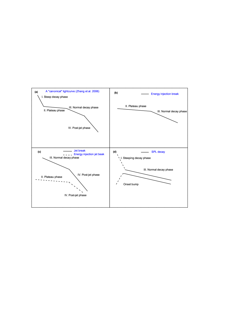
Figure 6: Typical light curve behaviors: (a) The canonical X-ray light curve, reproduced from Zhang et al (2006), with four characteristic temporal segments marked; (b) The energy injection break case, with a transition from the shallow decay phase (segment II) to the normal decay phase (segment III); (c) The jet break cases without (solid) or with (dashed) energy injection. For the former, it is a transition from the normal decay phase (segment III) to the post-jet-break phase (segment IV); for the latter, both segments have a shallower decay slope; (d) the single power-law (SPL) case. The steep decay phase in the X-ray light curve and the early rising phase in the optical light curve are not included in the analysis.

For the time domain we are interested in and for the optical and X-ray bands, there are four types of lightcurves (Fig.6):

(1) Broken power-law lightcurves with an energy injection break: In reference of the canonical X-ray light curve (Zhang et al. 2006), as reproduced in Fig.6(a), the energy injection break connects the shallow decay phase (segment II) to the normal decay phase (segment III), and a typical light curve is shown in Figure 6(b). Before and after the break, the adiabatic deceleration $\alpha(\beta)$ relations with and without energy injection (as listed in Table 2, Zhang et al. 2006; Gao et al. 2013) are used to check whether the data are consistent with model predictions.

(2) Broken power-law lightcurves with a jet break: This corresponds to transition from segment III to IV in the canonical lightcurve, and a typical light curve is shown in Figure 6(c) upper curve. Lightcurves of such a category should satisfy the constant-energy, isotropic closure relations before the break, and the edge-effect post-jet-break closure relations after the break, with no energy injection effect both before and after the break (Table 2). The post-break decay index is required to be steeper than 1.5 for this model.

(3) Broken power-law lightcurves with a jet break with energy injection: This model allows the energy injection extend to a duration longer than the jet break. The temporal break is still defined by the edge effect of a canonical jet, but the decay slopes before and after the break are shallower than the previous case (lower curve in Fig.6(c)), so that a $q$ parameter is introduced for both pre- and post-break phases.

(4) Single power-law decay: For some GRBs, a SPL function is adequate to describe the afterglow data (Figure 6(d)) after the deceleration phase. In the X-ray band, there might be a steeper decay phase before this SPL phase, which is due to the tail emission from the prompt emission (Tagliaferri et al., 2005; Barthelmy et al., 2005; Zhang et al., 2006). We ignore the steep decay phase and treat it as a SPL decay (upper curve of Fig.6(d)). Similarly, in the optical band, some GRBs show an early rising phase, which is a signature of the onset of afterglow at the deceleration radius (peak of the lightcurve, lower curve of Fig.6(d)). We treat these lightcurves also as SPL decay ones.

For all the types, sometimes there are X-ray flares overlapping on the power-law decay segments. We do not include the flares in our data fitting, since they originate from a different emission component due to late central engine activities (e.g., Zhang et al., 2006; Maxham & Zhang, 2009).

One important task is to perform a self-consistency check between the optical and X-ray bands. If a GRB is consistent with the external forward shock model, we demand that the GRB satisfies the following criteria:

• The X-ray and optical lightcurves are consistent with having an achromatic break if any;

• Both the X-ray and optical lightcurves should satisfy closure relations of a same circumburst medium type (ISM or wind) in both pre- and post-break temporal segments;

• Either both bands belong to the same spectral regime, or the two bands are separated by a cooling break $\nu_{c}$, with the X-ray band above the break and the optical band below the break (with allowance of a grey zone, see more discussion below);

• The inferred electron spectral index $p$ from both bands and from both pre- and post-break segments should be consistent with each other within error;

• For energy injection models, the energy injection parameter $q$ values derived from the X-ray and optical bands should be consistent with each other.

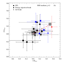
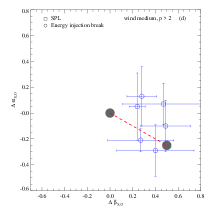
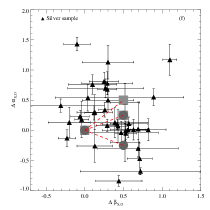
Figure 7: The confrontation of the data with model predictions in the $\Delta\beta_{\rm X,O}-\Delta\alpha_{\rm X,O}$ plane. The ($\Delta\beta_{X,O}$, $\Delta\alpha_{X,O}$) model predictions for the ISM and wind medium in different spectral regimes are denoted as large grey symbols: squares for ISM and circles for wind, respectively. The red dashed lines define the ($\Delta\beta_{X,O}$, $\Delta\alpha_{X,O}$) range for the grey zones. The SPL, energy injection, and jet break samples are presented by square, circle, and star, respectively. The ISM and wind samples are marked with filled and open symbols, respectively. The X-ray and optical bands in the same spectral regime, different spectral regimes, and grey zone are marked with black, red, and blue, respectively. (a): the entire Gold sample GRBs; (b)and (c): the ISM models with $p>2$ and $1<p<2$, respectively; (d) and (e): ththe wind models with $p>2$ and $1<p<2$, respectively; (f): the silver sample GRBs (denoted in triangles).

Technically, we check the consistency between the closure relations for individual temporal segment in individual energy band. To ensure a same $p$ value derived for different bands, we also check the consistency between the data and models in the $\bigtriangleup\beta_{\rm X,O}-\bigtriangleup\alpha_{\rm X,O}$ plane. Here $\bigtriangleup\alpha_{\rm X,O}=\alpha_{\rm X}-\alpha_{\rm O}$ is the difference between the decay indices in the X-ray and optical bands, respectively, in a same temporal segment, and $\bigtriangleup\beta_{\rm X,O}=\beta_{X}-\beta_{O}$ is the difference between the spectral indices in the X-ray and optical bands, respectively. Based on the closure relations (Table 2), one can derive the $\bigtriangleup\beta_{\rm X,O}-\bigtriangleup\alpha_{\rm X,O}$ relations of all the models (Table 3 and 4). One can see that even though $\alpha$ and $\beta$ values can be very different in different models, the $\Delta\alpha_{\rm X,O}$ and $\Delta\beta_{\rm X,O}$ values have several well-predicted values. In particular, for the SPL, and jet break models, both pre- and post-break values are well-defined constants. For the energy injection breaks, the post-break segment does not depend on the free parameter $q$. As a result, if one focuses on the second component only, all the models can be expressed as several representative coordinate values in the $\bigtriangleup\beta_{\rm X,O}-\bigtriangleup\alpha_{\rm X,O}$ plane. Considering the possible grey zones (see below for details), these points define several straight lines in the $\bigtriangleup\beta_{\rm X,O}-\bigtriangleup\alpha_{\rm X,O}$ space (Fig.7 for details). If the observed data intersect with these model lines (within error), one can regard them as being consistent with the model predictions.

Take the energy injection break as an example, our analysis uses the following procedure: (a) Use the observed spectral indices $\beta_{\rm O}$ and $\beta_{\rm X}$ to predict the post-break temporal indices $\alpha_{\rm O,2}$ and $\alpha_{\rm X,2}$ in two possible spectral regimes. Then compare these theoretical predictions with the observational values. If theoretical values are consistent with the fitting results within error then go to next step. Otherwise, it indicates that this GRB does not fall into this light curve type; (b) Use the identified spectral regime to calculate the electron spectral index $p$ from the spectral index $\beta$, i.e. $p=2\beta+1$ for $\nu_{m}<\nu<\nu_{c}$, or $p=2\beta$ for $\nu>\nu_{c}$. Compare the $p$ values derived from the optical and X-ray data, respectively. If $p_{\rm O}=p_{\rm X}$ within error, then move to the next step. Otherwise, this GRB does not fall into such a light curve type; (c) Use the inferred $p$ value and spectral regimes to infer the energy injection parameter $q$ using the temporal index before the break ($\alpha_{\rm O,1}$ and $\alpha_{\rm X,1}$). Compare the derived $q$ values from optical and X-ray bands, respectively. If $q_{\rm O}=q_{\rm X}$ within error, then move to the next step. Otherwise, this GRB does not fall into such a light curve type; (d) Using the $\bigtriangleup\beta_{\rm X,O}-\bigtriangleup\alpha_{\rm X,O}$ relation to double check the data, if the data fall into the predicted region in the $\bigtriangleup\beta_{\rm X,O}-\bigtriangleup\alpha_{\rm X,O}$ plane, then this burst can be fully interpreted by such a model. Otherwise, the burst does not fall into this category.

The simplest analytical model (Sari et al. 1998) predicts $\beta=p/2$ for Regime I ($\nu>\nu_{c}$) and $\beta=(p-1)/2$ for Regime II ($\nu_{m}<\nu<\nu_{c}$). Detailed numerical calculations (Uhm & Zhang, 2014a) showed that the transition between the two regimes may take several orders of magnitude in observer time. As a result, some “grey zones”, with $(p-1)/2<\beta<p/2$ are allowed by the model. Therefore the parameter space between the two closure relation lines defined by the two spectral regimes in the $\alpha-\beta$ plane is allowed by the theory. Data points falling into this grey zone should be regarded as consistent with the model. There are three possibilities: (1) the optical band is in Regime II, while the X-ray band is in the grey zone; (2) the X-ray band is in Regime I, while the optical band is in the grey zone; and (3) both bands are in the grey zone.

For the cases that both the optical and X-ray bands are in the same spectral regime, we demand that three spectral indices be the same within error, i.e. $\beta_{\rm O}=\beta_{\rm OX}=\beta_{\rm X}$, where $\beta_{\rm OX}$ is the spectral index between the optical and X-ray band in the joint spectral energy distribution (SED). If the two bands are in different spectral regimes, we demand $\beta_{\rm O}<\beta_{\rm OX}\leq\beta_{\rm X}$ or $\beta_{\rm O}\leq\beta_{\rm OX}<\beta_{\rm X}$.

4 Confronting Data with Models

4.1 Grading criteria and sample definitions

With the above preparation, everything is in place for us to systematically confront the broad-band data with the external forward shock afterglow models. Based on how badly the data violate the models, we define the following five grades (see also Table 5):

• Grade I: Both X-ray and optical bands have SPL lightcurves or BPL lightcurves with an acceptable achromatic break. Both bands satisfy closure relations and are self-consistent (same medium type, $p$ and $q$ values). These are the best examples where the GRB afterglow data abide by the external shock model predictions;

• Grade II: Some GRBs have a clear break at $t_{b}$ in one band (e.g., X-rays), but do not have a break in another band (e.g., optical). The missing break is likely due to incomplete observational coverage before or after the break. The data are consistent with the hypothesis of an achromatic break, and both bands satisfy closure relations self-consistently. These GRBs are almost as good as Grade I in terms of abiding by the external shock models;

• Grade III: Both X-ray and optical bands have SPL lightcurves or BPL lightcurves with an acceptable achromatic break. However, at least one temporal segment in one band does not satisfy the closure relations in a self-consistent manner with respect to other segments/band.

• Grade IV: This is the Grade II equivalent for Grade III. One band does not have a break, but the data are consistent with the hypothesis of having an achromatic break. At least one temporal segment in one band does not satisfy the closure relations in a self-consistent manner with respect to other segments/band.

• Grade V: Clear evidence of chromatic breaks and violation of closure relations. These GRBs cannot be interpreted within the one-component external shock models.

With these five grades, we define three samples:

• Gold Sample: The GRBs in Grade I and II are defined as the Gold sample GRBs, since no observed information violates any predictions of the external shock models;

• Silver Sample: The GRBs in Grade III and IV are included in this sample. Even though at least one segment/band does not satisfy the closure relations self-consistently, the basic requirement of achromaticity is not violated. We note that the closure relations are the predictions of the simplest analytical external forward shock models. More complicated models invoking, e.g., a structured jet (Zhang & Mészáros, 2002; Rossi et al., 2002; Kumar & Granot, 2003; Granot & Kumar, 2003) or a circumburst density medium with an arbitrary $k$ value (at least for a certain distance range), predict light curve behaviors that may not fully abide by the simple closure relations. Furthermore, if the GRB engine is long-lived and a long-lasting reverse shock outshines the forward shock, a variety of rich light curve behaviors can be generated, which do not follow the simple closure relations (e.g., Uhm et al., 2012; Uhm & Zhang, 2014b). So it is possible that the GRBs in the silver sample are still consistent with the external shock models;

• Bad Sample: The GRBs in Grade V violate the basic achromaticity principle of the external shock models and do not abide by the closure relations, and therefore cannot be interpreted within the framework of the external shock models.

4.2 Grading results

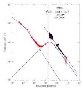
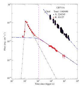
Figure 4: Same as Figure 1, but for the Grade IV sample

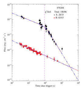
Figure 5: Same as Figure 1, but for the Grade V sample

The 85 well-sampled GRBs in our sample are graded based on the above-defined grading criteria. The GRBs in the five grades are presented in Figures 1 - 5, respectively. The relevant data of different grades are presented in Table 1 and 6.

• Grade I: As can be seen from Table 1 and 6, and Figure 1, within errors 43/85 GRBs satisfy the Grade I criteria. Out of 43 GRBs, 13, 8 and 22 GRBs are constrained to have an energy injection break, jet break and SPL decay, respectively.

• Grade II: within error 2/85 GRBs fall into this grade (Fig.2).

• Grade III: there are 34/85 GRBs falling into this grade (Fig.3). Among the sample, 15/34 and 19/34 GRBs have SPL and BPL lightcurves, respectively. GRBs 060906, 080319B and 100219A have two beaks at different times, respectively.

• Grade IV: there are 3/85 GRBs falling into this grade (Fig.4).

• Grade V: there are 3/85 GRBs falling into this grade (Fig.5). Two of them (GRBs 060607A and 070208) show clear chromatic breaks with good temporal coverage in both bands at the break times. One GRB (GRB 070420) shows a chromatic behavior based on the available data and simple model fitting, even though no observational data are available in the optical band at the break time of the X-ray band, so that the existence of a break in the optical band (even though very contrived in shape) at the same epoch is not completely ruled out.

Consequently, we get three samples:

• Gold sample: This sample has 45/85 GRBs, including 13/49, 8/49 and 24/49 GRBs satisfying the energy injection, jet break, jet break with energy injection, and SPL decay models, respectively. Among them, 27/49 and 18/49 are consistent with the ISM and wind models, respectively; 17/49, 4/49 and 24/49 GRBs are consistent with being in a same spectral regime, different spectral regimes (X-ray band in regime I and optical band in regime II), and grey zone, respectively. Among the 17 GRBs with the same spectral regime, 15 and 2 GRBs are consistent with being in the ISM II and wind II spectral regimes, respectively. For the 4 GRBs with different spectral regime, all of them are consistent with having an ISM medium.

• Silver sample: This sample has 37/85 GRBs, which may (or may not) be interpreted within the more complicated numerical external shock models.

• Bad sample: Only 3/85 GRBs definitely violate the basic achromaticity principle of the external shock models and therefore belong to the bad sample.

Figure 7a shows $\bigtriangleup\beta_{\rm X,O}-\bigtriangleup\alpha_{\rm X,O}$ distributions for Gold sample. For the energy injection sample, we only used the post-break segment to remove the $q$-dependence. These are the GRBs that also satisfy the closure relations in all temporal segments. We do not show the closure relation $\alpha-\beta$ plots since the energy injection models have an extra $q$-dependence on the $\alpha$ values. To show the details of how each burst may fall into the model predictions of each model (grey zone included), in Figure 7(b-e) we show the $\bigtriangleup\beta_{\rm X,O}-\bigtriangleup\alpha_{\rm X,O}$ distributions of those Gold-Sample GRBs that satisfy the ISM and wind medium models with $p>2$ and $1<p<2$, respectively. The Silver sample GRBs are collected in Figure 7f). About half of them fall outside the predicted region (red box) defined by the models. Even though some fall into the box, they do not satisfy the closure relations in all the temporal segments in all energy bands.

5 Statistics of the External Shock Afterglow Model Parameters

Since the Gold sample (Grade I and II) GRBs comply with the external shock models well, they serve as an excellent sample to study external shock model parameters. The derived external shock parameters of the Gold sample GRBs are presented in Table 6. We present some statistical properties of these model parameters in this section.

5.1 Temporal indices $\alpha$

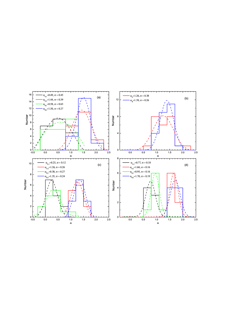
Figure 8: The distributions of the temporal decay index $\alpha$ for various sub-samples in the Gold sample and their best Gaussian fits (dashed curves): (a) all the BPL GRBs in the Gold sample, with best fits $\alpha_{\rm O,1}=0.49\pm 0.45$, $\alpha_{\rm O,2}=1.44\pm 0.39$, $\alpha_{\rm X,1}=0.58\pm 0.63$, and $\alpha_{\rm X,2}=1.50\pm 0.27$; (b) all the SPL GRBs in the Gold sample, with best fits $\alpha_{\rm O}=1.26\pm 0.38$, $\alpha_{\rm X}=1.39\pm 0.26$; (c) the energy injection sample, with $\alpha_{\rm O,1}=0.25\pm 0.12$, $\alpha_{\rm O,2}=1.26\pm 0.26$, $\alpha_{\rm X,1}=0.30\pm 0.27$, and $\alpha_{\rm X,2}=1.35\pm 0.24$; (d) the jet break sample, with $\alpha_{\rm O,1}=0.77\pm 0.18$, $\alpha_{\rm O,2}=1.66\pm 0.16$, $\alpha_{\rm X,1}=0.95\pm 0.16$ and $\alpha_{\rm X,2}=1.70\pm 0.19$.

Figure 8 shows the distributions of the temporal indices $\alpha$ in different energy bands and different temporal segments. They are all well fitted with Gaussian distributions for each band/temporal segment. For the GRBs having a BPL lightcurve, the typical $\alpha$ values are $\alpha_{\rm O,1}=0.49\pm 0.45$, $\alpha_{\rm O,2}=1.44\pm 0.39$, $\alpha_{\rm X,1}=0.58\pm 0.63$ and $\alpha_{\rm X,2}=1.50\pm 0.27$, respectively (Fig.8a). For the GRBs with a SPL lightcurve, one has $\alpha_{\rm O}=1.26\pm 0.38$, and $\alpha_{\rm X}=1.39\pm 0.26$ (Fig.8b). For the BPL sample, we also separate it into the energy injection sample and the jet break sample and perform the statistics. For the energy injection breaks, one has $\alpha_{\rm O,1}=0.25\pm 0.12$, $\alpha_{\rm O,2}=1.26\pm 0.26$, $\alpha_{\rm X,1}=0.30\pm 0.27$ and $\alpha_{\rm X,2}=1.35\pm 0.24$, respectively (Fig.8c). For the jet breaks, one has $\alpha_{\rm O,1}=0.77\pm 0.18$, $\alpha_{\rm O,2}=1.66\pm 0.16$, $\alpha_{\rm X,1}=0.95\pm 0.16$ and $\alpha_{\rm X,2}=1.70\pm 0.19$, respectively (Fig.8d). Both the pre-break and the post-break $\alpha$ values in the energy injection sample are systematically shallower than those in the jet break sample. On average, the X-ray lightcurves are steeper than the optical lightcurves, consistent with the expectations of the theoretical models (i.e. the X-ray band is more likely above $\nu_{c}$ while the optical band is more likely below $\nu_{c}$).

Another self-consistency check is to compare the observed change of decay slope, $\Delta\alpha=\alpha_{2}-\alpha_{1}$, with the model predictions. From the closure relations (Table 2), one can derive

• For energy injection breaks:

  $$\Delta\alpha=\cases{\frac{(1-q)(2+\beta)}{2},&ISM II ($p>2$)\cr\frac{(1-q)(19+2\beta)}{16},&ISM II ($1<p<2$) ,\cr\frac{(1-q)(1+\beta)}{2},&ISM I ($p>2$), wind II ($p>2$), wind I ($p>2$)\cr\frac{(1-q)(7+\beta)}{8},&ISM I ($1<p<2$)\cr\frac{(1-q)(5+2\beta)}{8},&wind II ($1<p<2$)\cr\frac{(1-q)(3+\beta)}{4},&wind I ($1<p<2$)\cr}$$ (5)

• For jet breaks:

  $$\Delta\alpha=\cases{\frac{3}{4},&ISM I and II ($p>2$ and $1<p<2$)\cr\frac{1}{2},&wind I and II ($p>2$ and $1<p<2$)\cr}$$ (6)

• For jet breaks with energy injection:

  $$\Delta\alpha=\cases{\frac{(q+2)}{4},&ISM II ($p>2$), ISM I ($p>2$ and $1<p<2$)\cr\frac{(3q+6)}{16},&ISM II ($1<p<2$),\cr\frac{q}{2},&wind II and wind I ($p>2$ and $1<p<2$)\cr}$$ (7)

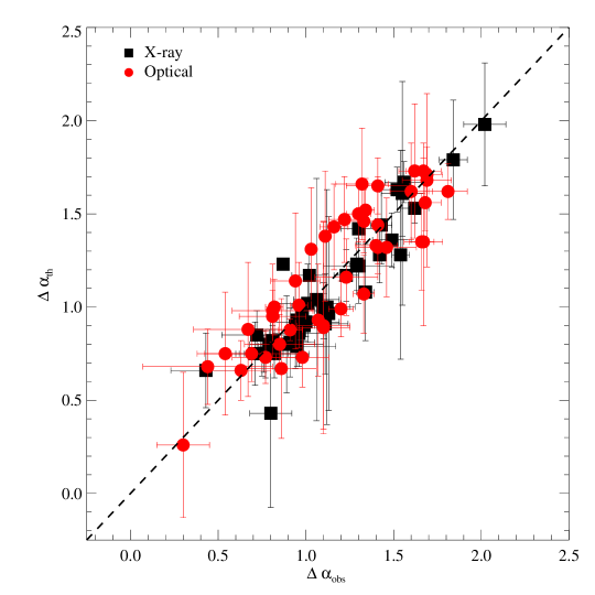
Figure 9: The observed temporal break change $\Delta\alpha=\alpha_{2}-\alpha_{1}$ compared against the theoretical value predicted from the closure relations. The square (black) and circle (red) data points correspond to X-ray and optical bands, respectively.

Figure 9 shows a comparison between the observed $\Delta\alpha_{\rm obs}$ and the theoretically predicted $\Delta\alpha_{\rm th}$ for each GRB derived from the measured $\beta$ and $q$ values using the corresponding closure relations. One can see that the two are consistent with each other.

Figure 10 displays the observed $\Delta\alpha$ distributions of various samples. For the Gold sample, the $\Delta\alpha$ distributions of optical and X-ray data are consistent with each other, i.e. $\Delta\alpha_{\rm O}=0.94\pm 0.23$ and $\Delta\alpha_{\rm X}=0.88\pm 0.28$ (Fig.10a). Furthermore, the $\Delta\alpha$ values of both bands in sub-groups (energy injection breaks and jet breaks) are also consistent with each other: $\Delta\alpha_{\rm O}=1.05\pm 0.17$ and $\Delta\alpha_{\rm X}=1.10\pm 0.21$ for the energy injection breaks, and $\Delta\alpha_{\rm O}=0.75\pm 0.22$ and $\Delta\alpha_{\rm X}=0.75\pm 0.22$ for the jet breaks (Fig.10b). The Silver sample, on the other hand, shows a poorer statistical behavior (Fig.10c and d).

5.2 Spectral indices $\beta$

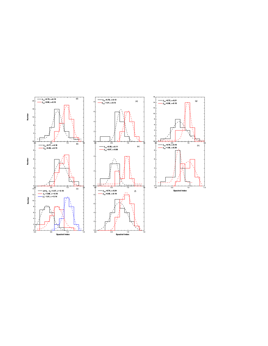
Figure 11: The distributions of the spectral indices $\beta$ of various sub-samples in the Gold sample and their best Gaussian fits (dashed curves): (a) the distributions for the entire Gold sample, with $\beta_{\rm O}=0.70\pm 0.15$, and $\beta_{\rm X}=0.98\pm 0.15$; (b) the $\beta$ distributions of the GRBs with optical and X-ray bands constrained in the same spectral regime, with $\beta_{\rm O}=0.77\pm 0.19$, $\beta_{\rm X}=0.89\pm 0.15$; (c) the $\beta$ distributions for the GRBs with optical and X-ray bands constrained in different spectral regimes, with $\beta_{\rm O}=0.68\pm 0.18$, $\beta_{\rm X}=1.01\pm 0.14$ and $\bigtriangleup\beta=\beta_{\rm X}-\beta_{\rm O}=0.37\pm 0.18$, which is consistent with the theoretical value 0.5 as expected for a cooling break; (d) the $\beta$ distributions for energy injection, with $\beta_{\rm O}=0.78\pm 0.12$, and $\beta_{\rm X}=1.01\pm 0.13$; (e) the $\beta$ distributions for the jet break sample, with $\beta_{\rm O}=0.59\pm 0.11$, and $\beta_{\rm X}=0.97\pm 0.08$; (f) the $\beta$ distributions for the SPL decay sample, with $\beta_{\rm O}=0.74\pm 0.24$, and $\beta_{\rm X}=0.95\pm 0.19$; (g) the $\beta$ distributions for the GRBs with an ISM medium, with $\beta_{\rm O}=0.72\pm 0.21$, and $\beta_{\rm X}=0.98\pm 0.10$; (h) the $\beta$ distributions for the GRBs with a wind medium, with $\beta_{\rm O}=0.70\pm 0.10$, and $\beta_{\rm X}=1.00\pm 0.20$.

Figure 11 shows the spectral index distributions for the Gold sample. In general, the distributions can be fitted with gaussian functions. For the global sample, one has $\beta_{\rm O}=0.70\pm 0.15$, and $\beta_{\rm X}=0.98\pm 0.15$ (Fig.11a). In the Gold sample, 17/45 GRBs have both the optical and X-ray bands in the same spectral regime. One has $\beta_{\rm O}=0.77\pm 0.19$, and $\beta_{\rm X}=0.89\pm 0.15$, which are consistent with each other (Fig.11b). The rest 28/45 GRBs are identified to have X-ray and optical bands separated by a cooling break. The results show $\beta_{\rm O}=0.68\pm 0.18$, $\beta_{\rm X}=1.01\pm 0.14$, with $\Delta\beta=\beta_{\rm X}-\beta_{\rm O}=0.37\pm 0.18$, which is consistent with the theoretically expected value $0<\Delta\beta\leq 0.5$ (Fig.11c).

We investigate the $\beta$ distributions in different types of lightcurves. For the energy injection sample, one has $\beta_{\rm O}=0.78\pm 0.12$, and $\beta_{\rm X}=1.01\pm 0.13$ (Fig.11d); for the jet break sample, one has $\beta_{\rm O}=0.59\pm 0.11$, and $\beta_{\rm X}=0.97\pm 0.08$ (Fig.11e); and for the SPL sample, one has $\beta_{\rm O}=0.74\pm 0.24$, and $\beta_{\rm X}=0.95\pm 0.19$ (Fig.11f).

We also investigate the $\beta$ distributions in different ambient medium types. For the ISM model (27/45 GRBs), one has $\beta_{\rm O}=0.72\pm 0.21$, and $\beta_{\rm X}=0.98\pm 0.10$ (Fig.11g); and for the wind model (18/45 GRBs), one has $\beta_{\rm O}=0.70\pm 0.10$, and $\beta_{\rm X}=1.00\pm 0.20$ (Fig.11h). The ISM model is more favored than the wind model, which is consistent with the previous results (e.g., Panaitescu & Kumar, 2002; Yost et al., 2003; Zhang et al., 2006; Schulze et al., 2011).

5.3 Electron spectral index $p$

Figure 12 shows the distributions of the electron spectral index $p$ of the Gold sample. It has a Gaussian distribution with $p=2.33\pm 0.48$ (Fig.12a), which is very consistent with the typical value of $p$ for relativistic shocks due to 1st-order Fermi acceleration (e.g., Achterberg et al., 2001; Ellison & Double, 2002). It also has a wide distribution, which is consistent with previous studies (e.g., Shen et al., 2006; Liang et al., 2007, 2008; Curran et al., 2010).

The $p$ distribution in different sub-samples are also generally consistent with each other. Within the Gold sample, those GRBs with optical and X-ray bands in the same spectral regime have $p=2.58\pm 0.39$, whereas those with optical and X-ray bands in different spectral regimes have $p=2.17\pm 0.44$ (Fig.12a). For the three light curve sub-samples, one has $p=2.34\pm 0.38$ for the energy injection break sample, $p=1.91\pm 0.37$ for the jet break sample, and $p=2.48\pm 0.47$ for the SPL sample, respectively (Fig.12b). For the two medium type models, one has $p=2.43\pm 0.57$ for the ISM model, and $p=2.28\pm 0.33$ for the wind model, respectively (Fig.12c).

5.4 Break time $t_{b}$

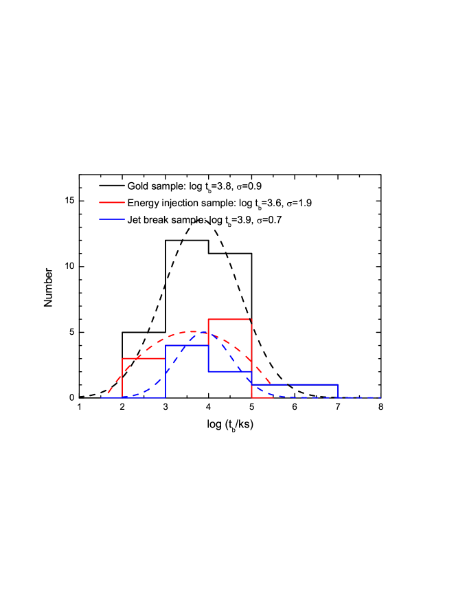
Figure 13: The distributions of the inferred $t_{\rm b}$ for the entire Gold sample, the energy injection sample, and the jet break sample. The dash lines are the best Gaussian fits: the entire Gold sample ($\rm log(t_{\rm b}\rm/ks)=(3.8\pm 0.9$)), the energy injection break sample ($\rm log(t_{\rm b}\rm/ks)=(3.6\pm 1.9$)) and the jet break sample ($\rm log(t_{\rm b}\rm/ks)=(3.9\pm 0.7$)).

Figure 13 shows the distributions of the observed achromatic break times, $t_{b}$. The global distribution in the Gold sample gives $\log(t_{b}\rm/ks)=(3.8\pm 0.9)$. Separating the energy injection sample and jet break sample, one has $\log(t_{b}\rm/ks)=(3.6\pm 1.9)$ for the energy injection break sample, $\log(t_{b}\rm/ks)=(3.9\pm 0.7)$ for the jet break sample. The energy injection ends (which depends on central engine) is on average earlier than the jet break time (which depends on geometry of the jet). The distribution of the energy injection break time is wider than the jet break time distribution.

5.5 Energy injection parameter $q$

Within the Gold sample, 13/45 GRBs show an energy injection type break, i.e. either an energy injection break or a jet break with energy injection. Among them, 4/13 and 9/13 GRBs satisfy the ISM and wind model, respectively. The distributions of the energy injection parameter $q$ of various samples are shown in Figure 14. The global sample has $q=0.22\pm 0.11$. The ISM and wind models have $q=0.20\pm 0.12$ and $q=0.23\pm 0.13$, respectively, which are consistent with each other.

5.6 Shock magnetic field equipartition factor $\epsilon_{B}$

Among the derived shock parameters, the magnetic field equipartition factor $\epsilon_{B}$ is of special interest. If the shock simply compresses the upstream magnetic field, then the expected $\epsilon_{B}$ is low, of the order of $10^{-6}-10^{-7}$. If, however, various plasma instabilities are playing a role to amplify the magnetic fields (e.g., Medvedev & Loeb, 1999; Nishikawa et al., 2009), one would expect a relatively large $\epsilon_{B}$ as high as 0.1. Early afterglow modeling (e.g., Wijers & Galama, 1999; Panaitescu & Kumar, 2001, 2002; Yost et al., 2003) derived a relatively large $\epsilon_{B}$, with a typical value $\sim 0.01$. On the other hand, modeling of GeV emission in several Fermi/LAT-detected GRBs led to the suggestion that $\epsilon_{B}$ should be relatively low at least for some GRBs (Kumar & Barniol Duran, 2009, 2010). Santana et al. (2014) derived $\epsilon_{B}$ for a large sample of GRBs, and derived a medium value of $10^{-5}$.

With our Gold sample, we can constrain $\epsilon_{B}$ independently. Even though in most GRBs, $\epsilon_{B}$ cannot be constrained due to the degeneracy of the data, one can still place interesting upper limits to $\epsilon_{B}$ based on the medium type and spectral regime of the GRBs. For example, in the ISM model $\nu_{c}$ decreases with time. For a regime II ($\nu_{m}<\nu<\nu_{c}$) GRB, the last data point in the light curve would set a lower limit on $\nu_{c}$ at that epoch, and hence, an upper limit on $\epsilon_{B}$. Similarly, in the wind model $\nu_{c}$ increases with time. For a regime II GRB, the first data point in the light curve would set a lower limit on $\nu_{c}$ at that point, and hence, an upper limit on $\epsilon_{B}$.

In the Appendix, we present expressions of $\nu_{m}$, $\nu_{c}$, $F_{\nu,\rm{max}}$ and the kinetic energy of the afterglow, $E_{\rm k,iso}$. For the $p>2$ cases, we adopt the formalism in previous works (Zhang et al., 2007a; Gao et al., 2013; Lü & Zhang, 2014). New expressions for the $1<p<2$ regime are also presented following Gao et al. (2013). We then derive the expressions of $\epsilon_{B}$ in various models, Eqs. (A6), (A9), (A20), and (A23), which are used to constrain $\epsilon_{B}$.

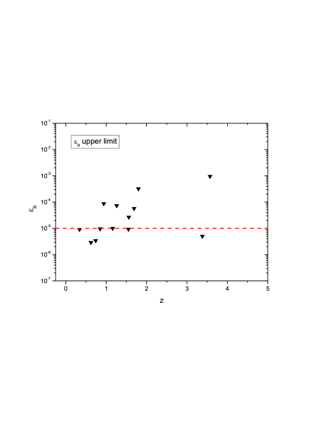
Figure 15: The derived upper limits of $\epsilon_{B}$ of GRBs that are in spectral regime II ($\nu_{m}<\nu<\nu_{c}$). Other parameters are fixed as $\epsilon_{e}=0.1$, $n=1$, and $A_{\ast}=1$. The dashed line denotes $\epsilon_{B}=10^{-5}$. Most GRBs are consistent with this value, with a few having upper limits even below this value.

The derived upper limits of $\epsilon_{B}$ are presented in Figure 15, with other parameters fixed as $\epsilon_{e}=0.1$, $n=1$ or $A_{\ast}=1$. One can see that in general these upper limits point towards a relatively low $\epsilon_{B}$ value. In some cases for the ISM model, the upper limits are even lower than $10^{-5}$. These results are consistent with the findings of Kumar & Barniol Duran (2009, 2010), Santana et al. (2014), and Barniol Duran (2014).

5.7 Energetics

The isotropic $\gamma$-ray energy $E_{\rm\gamma,iso}$ is calculated as

$$E_{\rm\gamma,iso}=\frac{4\pi D^{2}_{\rm L}S_{\gamma}k}{1+z},$$ (8)

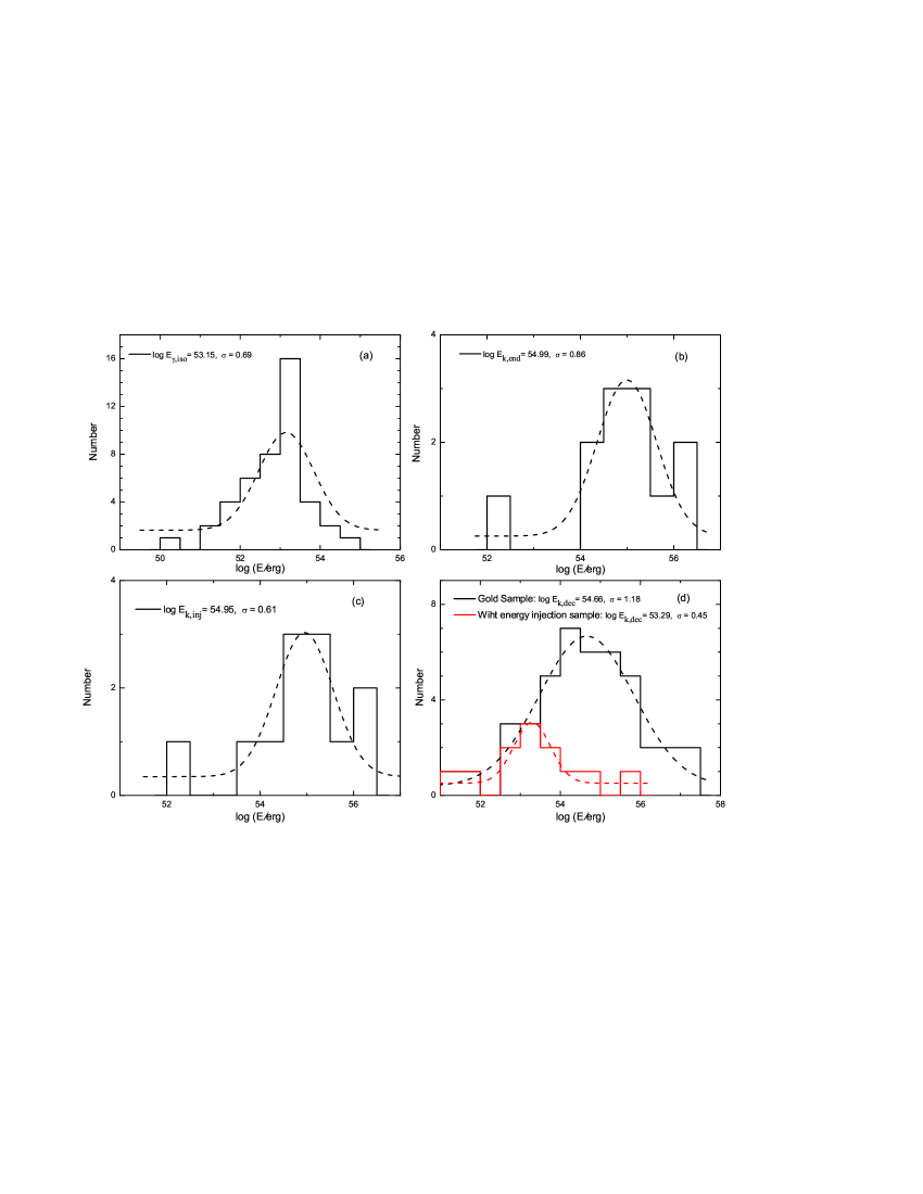
Figure 16: The distributions of various energy components derived from the Gold sample and their best Gaussian fits (dashed lines): (a) isotropic $\gamma$-ray energy, $E_{\rm\gamma,iso}$, with a typical value $\log(E_{\rm\gamma,iso}\rm/erg)=(53.15\pm 0.69)$; (b) the total isotropic kinetic energy at the end of energy injection for the energy injection sample, with a typical value $\log(E_{\rm K,end}\rm/erg)=(54.99\pm 0.86)$; (c) the distribution of the isotropic injected energy in the energy injection sample, with $\log(E_{\rm K,inj}\rm/erg)=(54.95\pm 0.61)$; (d) the isotropic kinetic energy at the deceleration time for the energy injection sample ($\log(E_{\rm K,dec}\rm/erg)=(53.29\pm 0.45)$), and for the entire Gold sample ($\log(E_{\rm K,dec}\rm/erg)=(54.66\pm 1.18)$). The following parameters are adopted in the kinetic energy calculations: $\epsilon_{e}=0.1$, $n=1$ or $A_{\ast}=1$, $Y=1$, and $\epsilon_{B}$ = $10^{-5}$.

where $S_{\rm\gamma}$ is the gamma-ray fluence in the BAT band, $D_{\rm L}$ is the luminosity distance of the source at redshift $z$, and the parameter $k$ is a factor to correct the observed $\gamma$-ray energy in a given band pass to a broad band (e.g., $1-10^{4}$ keV in the rest frame) with the observed GRB spectra (Bloom et al., 2001). It is well known that a typical GRB spectrum is well fitted with the so-called Band function (Band et al., 1993). If the Band parameters are measured for a burst, these parameters are used to derive the $k$ parameter. However, owing to the narrowness of the Swift/BAT band, the spectra of many Swift GRBs in our sample are adequately fitted with a single power-law, $N\propto E^{-\Gamma}$, so that the Band parameters are not well constrained. For these GRBs, we use an empirical relation between $E_{p}$ and BAT-band photon index $\Gamma$ (Zhang et al., 2007b; Sakamoto et al., 2009; Virgili et al., 2012) to estimate $E_{p}$. Taking typical values of the photon indices $\alpha=-1.1$ and $\beta=-2.2$ (Preece et al., 2000; Kaneko et al., 2006), we can derive $E_{\rm\gamma,iso}$ values of the GRBs with redshift measurements in our Gold sample, which range from $10^{51}$ to $10^{55}$ erg, with a typical value $\log(E_{\rm\gamma,iso}\rm/erg)=53.15\pm 0.69$ (Fig.16(a)).

The isotropic kinetic energy of the afterglow $E_{\rm K,iso}$ can be derived from the afterglow data. In general, broad-band modeling is needed to precisely measure $E_{\rm K,iso}$ (Panaitescu & Kumar, 2001, 2002). Most GRBs do not have adequate data to perform such an analysis. More conveniently, one may use the X-ray data only to constrain $E_{\rm K,iso}$, since the X-ray band is usually above $\nu_{c}$, so that the X-ray flux does not depend on the ambient density and only weakly depends on $\epsilon_{e}$ (Kumar, 1999; Freedman & Waxman, 2001; Berger et al., 2003; Lloyd-Ronning & Zhang, 2004; Zhang et al., 2007a), see Appendix for detailed derivations. For the cases with energy injection, $E_{\rm K,iso}$ is a function of time during the energy injection phase. Following Zhang et al. (2007a), we calculate $E_{\rm K,iso}$ at two different epochs, one at the break time $t_{b}$, when energy injection is over, and another at a putative deceleration time $t_{\rm dec}\sim{\rm max}(60~{}{\rm s},T_{90})$. We use the X-ray flux at $t_{b}$ to derive $E_{\rm K,end}$, and then derive $E_{\rm K,dec}=E_{\rm K,end}(t_{\rm dec}/t_{b})^{1-q}$. The total injected energy is calculated as $E_{\rm K,inj}=E_{\rm K,end}-E_{\rm K,dec}$. Based on our constraints on $\epsilon_{B}$, we take $\epsilon_{B}=10^{-5}$ for all the GRBs in our calculations. Other parameters are taken as typical values: $\epsilon_{e}=0.1$, $n=1$ or $A_{\ast}=1$, and $Y=1$.

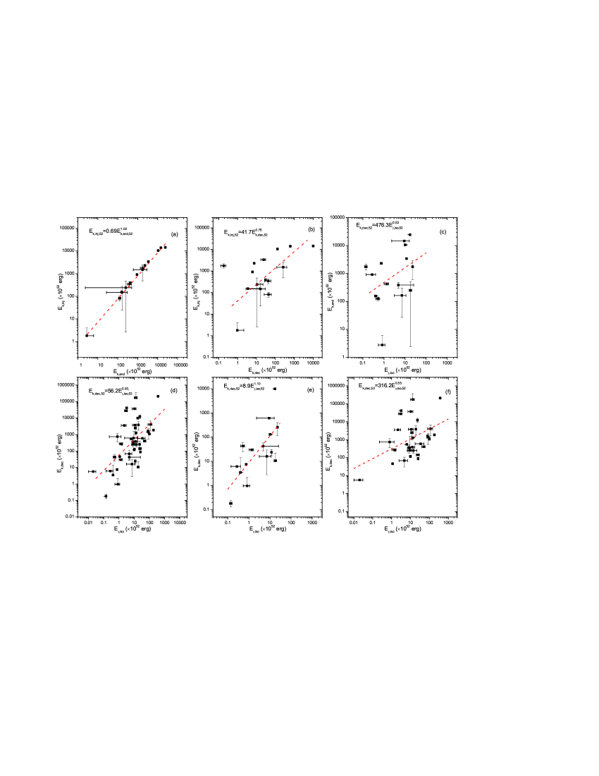
Figure 17: The correlations among different energy components: (a) $E_{\rm K,end}-E_{\rm K,inj}$: $E_{\rm K,inj,52}=0.69E^{1.02\pm 0.02}_{\rm K,end,52}$; (b) $E_{\rm K,dec}-E_{\rm K,inj}$: $E_{\rm K,inj,52}=41.7E^{0.76\pm 0.20}_{\rm K,dec,52}$; (c) $E_{\rm\gamma,iso}-E_{\rm K,end}$: $E_{\rm K,end,52}=476.3E^{0.53\pm 0.23}_{\rm\gamma,iso,52}$; (d), (e) and (f): $E_{\rm\gamma,iso}-E_{\rm K,dec}$ for the entire Gold sample, the energy injection sub-sample, and the sub-sample without energy injection, with $E_{\rm K,dec,52}=56.2E^{0.93\pm 0.19}_{\rm\gamma,iso,52}$, $E_{\rm K,dec,52}=8.9E^{1.10\pm 0.29}_{\rm\gamma,iso,52}$ and $E_{\rm K,dec,52}=316.2E^{0.55\pm 0.21}_{\rm\gamma,iso,52}$, respectively.

In Figure 16, we present several statistical results of the $E_{\rm K,iso}$ calculations. For the GRBs with energy injection, the distributions are log ($E_{\rm K,end}\rm/erg)=54.99\pm 0.86$ (Fig.16b), log ($E_{\rm K,inj}\rm/erg)=54.95\pm 0.61$ (Fig.16c), and log ($E_{\rm K,dec}\rm/erg)=53.29\pm 0.45$ (Fig.16d). For the entire Gold sample, one has log ($E_{\rm K,dec}\rm/erg)=54.66\pm 1.18$ (Fig.16d). It is interesting to see that the energetics of the energy-injection sample reache a similar level as the no-energy-injection sample after the energy injection is over. Clear correlations are found among different energy components: $E_{\rm K,end}-E_{\rm K,inj}$ relation $E_{\rm K,inj,52}=0.69E^{1.02\pm 0.02}_{\rm K,end,52}$ (Fig.17a), $E_{\rm K,dec}-E_{\rm K,inj}$ relation $E_{\rm K,inj,52}=41.7E^{0.76\pm 0.20}_{\rm K,dec,52}$ (Fig.17b), $E_{\rm\gamma,iso}-E_{\rm K,end}$ relation $E_{\rm K,end,52}=476.3E^{0.53\pm 0.23}_{\rm\gamma,iso,52}$ (Fig.17c), $E_{\rm\gamma,iso}-E_{\rm K,dec}$ relations in the entire Gold sample, $E_{\rm K,dec,52}=56.2E^{0.93\pm 0.19}_{\rm\gamma,iso,52}$ (Fig.17d), in the energy injection sample, $E_{\rm K,dec,52}=8.9E^{1.10\pm 0.29}_{\rm\gamma,iso,52}$ (Fig.17e), and in the no-energy-injection sample, $E_{\rm K,dec,52}=316.2E^{0.55\pm 0.21}_{\rm\gamma,iso,52}$ (Fig.17f), respectively. In particular, the$E_{\rm K,inj,52}=41.7E^{0.76\pm 0.20}_{\rm K,dec,52}$ correlation suggests a substantial energy injection during the shallow decay phase for most GRBs.

5.8 Radiative efficiency $\eta_{\gamma}$

The GRB radiative efficiency, defined as (Lloyd-Ronning & Zhang, 2004)

$$\eta_{\gamma}=\frac{E_{\rm\gamma,iso}}{E_{\rm\gamma,iso}+E_{\rm K,iso}},$$ (9)

is an essential parameter to probe how efficient a burst converts its global energy to prompt $\gamma$-ray emission. As mentioned above, if there is continuous energy injection, the kinetic energy of the afterglow $E_{\rm K,iso}$ takes different values if one chooses different epochs. In principle, $\eta_{\gamma}$ can be defined for two different epochs, $t_{\rm dec}$ and $t_{b}$, which have different physical meanings (see a discussion in Zhang et al. 2007a).

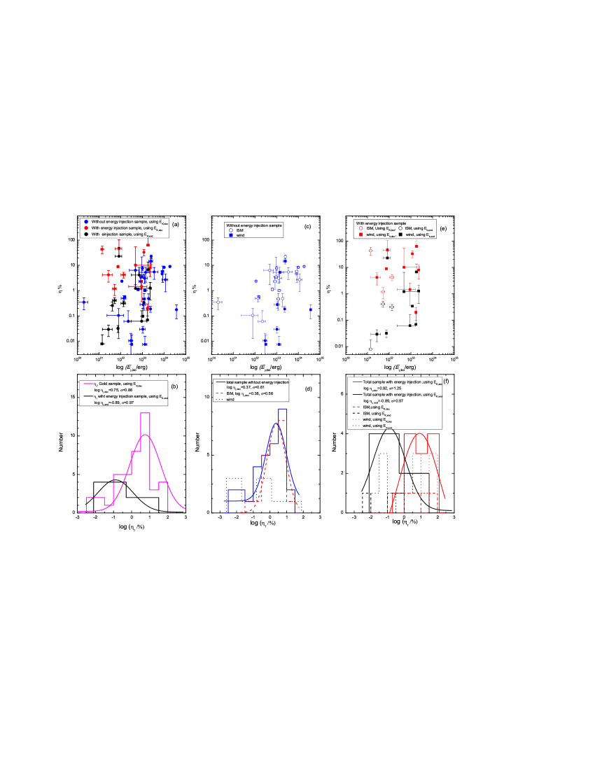
Figure 18: The radiative efficiency $\eta_{\rm\gamma}$ of the Gold sample as a function of $E_{\rm\gamma,iso}$ (upper row) and histograms (lower row): (a) and (b): For the entire Gold sample. Among them, the GRBs in the energy-injection sub-sample are marked in red and black. Two efficiencies are calculated for each GRB: one using $E_{\rm K,dec}$ (red) and the other using $E_{\rm end}$ (black). Those GRBs without energy injection are marked in blue. Log-normal fits to the efficiencies derived from $E_{\rm K,dec}$ and $E_{\rm end}$ give $\rm log(\eta_{\rm\gamma,dec}/\%)=0.75\pm 0.86$ and $\rm log(\eta_{\rm\gamma,end}/\%)=-0.89\pm 0.97$, respectively; (c) and (d): for the sub-sample of GRBs without energy injection, with best fit $\rm log(\eta_{\rm\gamma,dec}/\%)=0.36\pm 0.61$. Open circles denote the ISM medium and solid squares denote the wind medium; (e) and (f): for the sub-sample of GRBs with energy injection, with best fits $\rm log(\eta_{\rm\gamma,dec}/\%)=0.92\pm 1.25$ and $\rm log(\eta_{\rm\gamma,end}/\%)=-0.89\pm 0.97$, respectively. Again ISM and wind cases are denoted as open circles and solid squares, respectively.

Figure 18 shows the radiative efficiencies calculated at $t_{\rm dec}$ and $t_{b}$ as a function of $E_{\rm\gamma,iso}$ along with their histograms. No significant correlation between $\eta_{\gamma}$ and $E_{\rm\gamma,iso}$ is found. The fireball internal shock model predicts a relatively small efficiency of a few per cent (e.g., Kumar, 1999; Panaitescu et al., 1999; Maxham & Zhang, 2009; Gao & Mészáros, 2015). Previous constraints on GRB radiative efficiencies give relatively large values, as large as above $90\%$ (e.g., Lloyd-Ronning & Zhang, 2004; Zhang et al., 2007a; Racusin et al., 2011) for some GRBs. This challenges the internal shock models, and favors alternative prompt emission models, such as dissipation of magnetic fields (Zhang & Yan, 2011) or photospheric emission (Lazzati et al., 2013).

The derived efficiencies can be fit with rough log-normal distributions (Fig.18b, d, f). For the entire sample, one has $\rm log(\eta_{\rm\gamma,dec}/\%)=0.75\pm 0.86$. For the sub-sample GRBs without energy injection, the radiative efficiency is lower, with $\rm log(\eta_{\rm\gamma,dec}/\%)=0.37\pm 0.61$. For the sub-sample GRBs with energy injection, the radiative efficiencies read $\rm log(\eta_{\rm\gamma,dec}/\%)=0.92\pm 1.25$ for $t_{\rm dec}$, and $\rm log(\eta_{\rm\gamma,end}/\%)=-0.89\pm 0.97$ for $t_{b}$, respectively.

The derived efficiencies are somewhat smaller than the values derived in previous work (e.g. Zhang et al., 2007a). The main reason is the adoption of a smaller value of $\epsilon_{B}\sim 10^{-5}$, so that the derived $E_{\rm K,iso}$ are systematically larger. This greatly alleviates the low-efficiency problem of the internal shock models. Nonetheless, some GRBs still have tens of percent efficiency, which demands a contrived setup for the internal shock models (e.g., Beloborodov, 2000; Kobayashi & Sari, 2001). If $t_{\rm dec}$ is adopted, which is more natural for most prompt emission model to calculate efficiency (see Zhang et al. 2007a for a detailed discussion), $\eta_{\gamma}$ is still typically too large for the internal shock model. This is on the other hand consistent with the suggestion that internal collision-induced magnetic reconnection and turbulence (ICMART) is the dominant process to power GRB prompt emission in the majority of GRBs, which can typically gives tens of percent radiative efficiency (Zhang & Yan, 2011; Deng et al., 2015). This conclusion is also consistent with independent studies of modeling the GRB prompt emission spectrum (Uhm & Zhang, 2014c) and quasi-thermal photosphere emission component (Gao & Zhang, 2015).

5.9 Jet opening angle and geometrically-corrected gamma-ray energy

In the Gold sample, 8/45 GRBs show a jet break. These include five GRBs of without energy injection and one more with energy injection. The ambient medium type of all 6 GRBs is ISM. Five out of these six GRBs have redshift information (Table LABEL:table:jet).

Under the assumption of a conical jet, one can derive the jet opening angle based on observational data (Rhoads, 1999; Sari et al., 1999; Frail et al., 2001):

$$\theta_{j}=0.070~{}{\rm rad}~{}\left(\frac{t_{b}}{1\ \rm day}\right)^{3/8}\left(\frac{1+z}{2}\right)^{-3/8}\left(\frac{E_{\rm K,iso}}{10^{53}\ \rm ergs}\right)^{-1/8}\left(\frac{n}{0.1\ \rm cm^{-3}}\right)^{1/8}.$$ (10)

We then calculate the geometrically corrected $\gamma$-ray energy

$$E_{\gamma}=(1-\cos\theta_{j})E_{\rm\gamma,iso},$$ (11)

and kinetic energy

$$E_{\rm K}=(1-\cos\theta_{j})E_{\rm K,iso}.$$ (12)

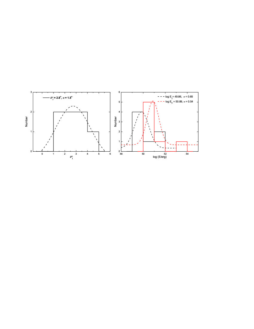
Figure 19: The distributions of the jet opening angle ($\theta_{j}$), geometrically corrected $\gamma$-ray energy ($E_{\rm\gamma}$) and kinetic energy ($E_{\rm K}$), respectively, derived from the jet break sub-sample of the Gold sample. The dashed lines are the best Gaussian fits, with $\theta_{j}=(2.8\pm 1.5)^{\rm o}$, $\log(E_{\rm\gamma}\rm/erg)=(49.86\pm 0.65)$, and $\log(E_{\rm K}\rm/erg)=(50.89\pm 0.54)$, respectively.

Here $E_{\rm K,iso}$ is taken as $E_{\rm K,end}$ for the energy injection sample. The medium density is taken as $n=1$ cm^-3.The results are presented in Table LABEL:table:jet and Figure 19. The best fitting results give $\theta_{j}=(2.8\pm 1.5)^{\rm\circ}$, $\log(E_{\gamma}/\rm erg)=49.86\pm 0.65$, and $\log(E_{\rm K}/\rm erg)=50.89\pm 0.54$.

6 Conclusions and Discussion

The chromatic afterglow behavior observed in some GRBs has raised the concern regarding whether the external forward shock models are still adequate to interpret the broad-band afterglows of GRBs and whether alternative ideas, e.g., a long-lasting engine-driven afterglow, are needed to account for the data. In order to answer “how bad/good the external shock models are”, in this paper, we systematically studied 85 Swift GRBs up to March 2014, which all have high-quality X-ray and optical light curves and spectral data to allow us to study the compliance of the data to the external forward shock models. The results of this study can be summarized as the following.

Based on how well the data abide by the external forward shock afterglow models, we categorized GRBs into five grades and three samples:

• A Gold sample (Grade I and II) includes 45/85 GRBs. These GRBs are fully consistent with the theoretical predictions of the external shock models, including having an acceptable achromatic break and fulfilling various closure relations between the temporal decay indices $\alpha$ and spectral indices $\beta$.

• A Silver sample (Grade III and IV) includes 37/85 GRBs. These GRBs are also consistent with having an acceptable achromatic break, even though one or more afterglow segments do not comply with the closure relations. These GRBs are potentially interpretable within the framework of external shock models.

• A Bad sample (Grade V) only includes 3/85 GRBs. These GRBs show direct evidence of chromatic behaviors, which cannot be accounted for within single-component external shock models.

The bottom line of this study is to address how bad/good the external shock models are. Our results show that external shock models work very well for at least $\sim$ 53% of GRBs (our Gold sample). These GRBs can be interpreted within the simplest afterglow models. If more advanced modeling invoking other factors (e.g., structured jet or long-lasting reverse shock) is carried out, up to $\sim 96\%$ of GRBs (including the Silver sample) may be accounted for within the external shock models. Only less than 4% GRBs truly violate the basic expectations of the external shock models, and demand another emission component (e.g., central engine afterglow) to account for emission in at least one band (e.g., the X-ray band).

Several caveats deserve mentioning. First, we only focused on the main afterglow components (SPL, BPL or TPL) of the X-ray and optical lightcurves. In some GRBs, there are additional components overlapping with these main components, such as the X-ray steep decay phase, X-ray flares, and optical re-brightening features, which are not included in the analysis. These features are usually chromatic, and demand additional emission components to interpret the data. The general conclusion that a lot of GRBs have extended central engine activities (Zhang et al., 2006) remain valid. The true duration of the GRB central engine activities may be much longer than what is measured by the GRB duration $T_{90}$ (Zhang et al., 2014). Second, we adopted a relatively “loose” criterion ( $\chi^{2}_{total}\leq 3$) to define “achromaticity” by requiring the X-ray and optical lightcurves to have a same break time. Searching for break times independently in the two bands often results in somewhat different break times, but many GRBs can be made being consistent with achromatic. The relatively large $\chi^{2}_{total}\sim 3$ in some GRBs is mostly caused by the additional features (small flares and fluctuations which we do not care) in the otherwise (broken) power law lightcurves. We therefore believe that our approach is appropriate to address the question of “how bad the models are”. On the other hand, if in the future high-quality data indeed show slight chromatic behaviors with high confidence, one should take cautious to the fraction numbers presented in this paper, and consider how such slight chromatic behaviors may impact the models. Finally, we only studied 85 GRBs that have both bright X-ray and bright optical emission data to allow us to perform the test. There are more GRBs detected by Swift ($\sim 900$ with X-ray lightcurves and $\sim 260$ with optical lightcurves). Due to the complicated sample selection effects, we do not guarantee that the fractions of Gold, Silver and Bad samples are reliable numbers for the entire GRB population. In any case, 85 GRBs represent a reasonably large sample, so that our statistics are valid at least for the “bright” sample of GRBs.

With the Gold sample, we further performed a series of statistical analyses of various observational properties and model parameters. Following interesting conclusions can be drawn:

• Temporal index $\alpha$: The temporal indices $\alpha$ in different bands and different temporal segments satisfy the afterglow model predictions. On average, the X-ray lightcurves are steeper than optical. For BPL lightcurves, the degrees of the break, $\Delta\alpha$, are consistent with the theoretical predictions of the energy injection models or jet break models;

• Spectral index $\beta$: The spectral indices $\beta$ in the optical and X-ray bands are $\beta_{O}=0.70\pm 0.15$, $\beta_{X}=0.98\pm 0.15$, respectively. Some (17/45) have X-ray and optical bands in the same spectral segment, while most (28/45) have the two bands separated by $\nu_{c}$ or in the grey zone. Statistically, $\Delta\beta=0.37\pm 0.18$ is consistent with the theoretical value 0-0.5, a range of $\Delta\beta$, including those expected in the grey zone (Uhm & Zhang, 2014a).

• Electron spectral index $p$: The typical value $p=2.33\pm 0.48$ is very consistent with the theoretical predictions for relativistic shocks. A wide range of $p$ values are observed, which is consistent with previous findings.

• Break time $t_{b}$: The typical break time is found to be $\log(t_{b}\rm/ks)=3.8\pm 0.9$. The break time of energy injection sample ($\log(t_{b}\rm/ks)=3.96\pm 1.9$) is statistically earlier than that of the jet break break sample ($\log(t_{b}\rm/ks)=3.9\pm 0.7$).

• Energy injection parameter $q$: the central value is $q=0.22\pm 0.11$, and the ISM and wind models are consistent with each other, with $q=0.20\pm 0.12$ and $q=0.23\pm 0.13$, respectively.

• Magnetization parameter $\epsilon_{B}$: The derived upper limits of $\epsilon_{B}$ suggests that the typical value of this parameter is low (say, $10^{-5}$), which is consistent with previous work (Kumar & Barniol Duran, 2009, 2010; Santana et al., 2014; Barniol Duran, 2014).

• Energetics: The typical isotropic $\gamma$-ray energy is $\log(E_{\rm\gamma,iso}\rm/erg)=53.15\pm 0.69$. For the energy injection case, the typical isotropic kinetic energy in the blastwave is log ($E_{\rm K,dec}\rm/erg)=53.29\pm 0.45$ at the deceleration time, and log ($E_{\rm K,end}\rm/erg)=54.99\pm 0.86$ when energy injection is over. For GRBs without energy injection, the typical blastwave kinetic energy is log ($E_{\rm K,dec}\rm/erg)=54.66\pm 1.18$. Clear correlations among various energy components are found.

• Radiative efficiency $\eta_{\gamma}$: With a small $\epsilon_{B}\sim 10^{-5}$ adopted, the derived radiative efficiency $\eta_{\gamma}$ is lower than previous studies. For the entire Gold sample, $\rm log(\eta_{\rm\gamma,dec}/\%)=0.75\pm 0.86$. Yet, the efficiency is still large for some GRBs, especially the ones with energy injection. For these GRBs, the efficiency measure at the deceleration time has $\rm log(\eta_{\rm\gamma,dec}/\%)=0.92\pm 1.25$, which still challenges the internal shock model.

• Jet opening angle $\theta_{j}$: For the jet break sample, we derived the typical jet opening angle as $\theta_{j}=(2.5\pm 1.5)^{\rm\circ}$. The jet-corrected $\gamma$-ray energy and kinetic energy are $\log(E_{\gamma}\rm/erg)=49.86\pm 0.65$ and $\log(E_{\rm K}\rm/erg)=50.89\pm 0.54$, respectively.

Appendix A Expressions of $E_{\rm K,iso}$ and $\epsilon_{B}$

In this Appendix, we present expressions of $E_{\rm K,iso}$ and $\epsilon_{B}$ of the external forward shock afterglow models.

A.1 The ISM model

For the $p>2$ case, the forward shock emission can be characterized as (Yost et al., 2003; Zhang et al., 2007a)

$$\nu_{m}=3.3\times 10^{12}~{}{\rm Hz}~{}\left(\frac{p-2}{p-1}\right)^{2}(1+z)^{1/2}\epsilon_{B,-2}^{1/2}\epsilon_{e,-1}^{2}E_{\rm K,iso,52}^{1/2}t_{d}^{-3/2},$$

$$\nu_{c}=6.3\times 10^{15}~{}{\rm Hz}~{}(1+z)^{-1/2}(1+Y)^{-2}\epsilon_{B,-2}^{-3/2}E_{\rm K,iso,52}^{-1/2}n^{-1}t_{d}^{-1/2},$$

$$F_{\nu,\rm{max}}=1.6~{}{\rm mJy}~{}(1+z)D^{-2}_{28}\epsilon_{B,-2}^{1/2}E_{\rm K,iso,52}n^{1/2},$$ (A1)

where $E_{\rm K,iso,52}$ is the isotropic kinetic energy (in units of $10^{52}$ erg) in the blastwave, $t_{d}$ is the time since trigger (in units of days), $n$ is the density of the constant ambient medium, $D_{L}=10^{28}~{}{\rm cm}~{}D_{28}$ is the luminosity distance, and

$$Y=[-1+(1+4\eta_{1}\eta_{2}\epsilon_{e}/\epsilon_{B})^{1/2}]/2$$ (A2)

is the inverse Compton parameter, with $\eta_{1}={\rm min}[1,(\nu_{c}/\nu_{m})^{(2-p)/2}]$ (Sari & Esin, 2001), and $\eta_{2}\leq 1$ is a correction factor introduced by the Klein-Nishina correction.

For $p>2$ and in the $\nu>\rm{max}(\nu_{m},\nu_{c})$ regime, one has (Zhang et al., 2007a)

$$\nu F_{\nu}(\nu=10^{18}~{}\rm{Hz}) = F_{\nu,\rm max}\nu_{c}^{1/2}\nu_{m}^{(p-1)/2}\nu_{X}^{(2-p)/2}$$ (A3)

$$= 5.2\times 10^{-14}~{}{\rm erg~{}s^{-1}~{}cm^{-2}}~{}D^{-2}_{28}(1+z)^{(p+2)/4}(1+Y)^{-1}f_{p1}\epsilon_{B,-2}^{(p-2)/4}\epsilon_{e,-1}^{p-1}$$

$$\times E_{\rm K,iso,52}^{(p+2)/4}t_{d}^{(2-3p)/4}\nu_{18}^{(2-p)/2},$$

where $\nu f_{\nu}(\nu=10^{18}Hz)$ is the energy flux at $10^{18}$ Hz (in units of ergs s^-1 cm^-1), and

$$f_{p1}=6.73\left(\frac{p-2}{p-1}\right)^{p-1}(3.3\times 10^{-6})^{(p-2.3)/2}$$ (A4)

is a function of electron spectral index $p$ (Zhang et al., 2007a). One can then derive

$$E_{\rm K,iso,52} = \left(\frac{\nu F_{\nu}(\nu=10^{18}~{}\rm{Hz})}{5.2\times 10^{-14}~{}{\rm erg~{}s^{-1}~{}cm^{-2}}}\right)^{4/(p+2)}D^{8/(p+2)}_{28}(1+z)^{-1}(1+Y)^{4/(p+2)}f_{p1}^{-4/(p+2)}\epsilon_{B,-2}^{(2-p)/(p+2)}$$ (A5)

$$\times\epsilon_{e,-1}^{4(1-p)/(p+2)}t_{d}^{(3p-2)/(p+2)}\nu_{18}^{2(p-2)/(p+2)},$$

$$\epsilon_{B,-2} = \left(\frac{6.3\times 10^{15}~{}\rm{Hz}}{\nu_{c}}\right)^{(p+2)/(p+4)}\left(\frac{\nu F_{\nu}(\nu=10^{18}~{}\rm{Hz})}{5.2\times 10^{-14}\rm{erg~{}s^{-1}~{}cm^{-2}}}\right)^{-2/(p+4)}D^{-4/(p+4)}_{28}$$ (A6)

$$\times(1+Y)^{-2(p+3)/(p+4)}n^{-(p+2)/(p+4)}f_{p1}^{2/(p+4)}\epsilon_{e,-1}^{2(p-1)/(p+4)}t_{d}^{-2p/(p+4)}\nu_{18}^{(2-p)/(p+4)}.$$

For $p>2$ and in the $\nu_{m}<\nu<\nu_{c}$ regime, one has

$$\nu F_{\nu}(\nu=10^{18}~{}{\rm Hz}) = F_{\nu,\rm max}\nu_{m}^{(p-1)/2}\nu_{X}^{(3-p)/2}$$ (A7)

$$= 6.5\times 10^{-13}~{}{\rm erg~{}s^{-1}~{}cm^{-2}}~{}D^{-2}_{28}(1+z)^{(p+3)/4}f_{p1}\epsilon_{B,-2}^{(p+1)/4}\epsilon_{e,-1}^{p-1}E_{\rm K,iso,52}^{(p+3)/4}$$

$$\times n^{1/2}t_{d}^{(3-3p)/4}\nu_{18}^{(3-p)/2},$$

so that

$$E_{\rm K,iso,52} = \left(\frac{\nu F_{\nu}(\nu=10^{18}~{}\rm{Hz})}{6.5\times 10^{-13}\rm{erg~{}s^{-1}~{}cm^{-2}}}\right)^{4/(p+3)}D^{8/(p+3)}_{28}(1+z)^{-1}f_{p1}^{-4/(p+3)}\epsilon_{B,-2}^{-(p+1)/(p+3)}$$ (A8)

$$\times\epsilon_{e,-1}^{4(1-p)/(p+3)}n^{-2/(p+3)}t_{d}^{(3p-3)/(p+3)}\nu_{18}^{2(p-3)/(p+3)},$$

$$\epsilon_{B,-2} = \left(\frac{6.3\times 10^{15}~{}\rm{Hz}}{\nu_{c}}\right)^{(p+3)/(p+4)}\left(\frac{\nu F_{\nu}(\nu=10^{18}~{}\rm{Hz})}{6.5\times 10^{-13}~{}{\rm erg~{}s^{-1}~{}cm^{-2}}}\right)^{-2/(p+4)}D^{-4/(p+4)}_{28}$$ (A9)

$$\times(1+Y)^{-2(p+3)/(p+4)}n^{-(p+2)/(p+4)}f_{p1}^{2/(p+4)}\epsilon_{e,-1}^{2(p-1)/(p+4)}t_{d}^{-2p/(p+4)}\nu_{18}^{(3-p)/(p+4)}$$

Following Gao et al. (2013), below we derive the expressions in the $p<2$ case.

In the $\nu>\rm{max}(\nu_{m},\nu_{c})$ regime, one has

$$E_{\rm K,iso} = (\nu F_{\nu}(\nu=10^{18}~{}{\rm Hz}))^{16/(p+14)}D^{32/(p+14)}f_{p2}^{-16/(p+14)}n^{(p-2)/(p+14)}t^{(3p+10)/(p+14)}(1+Y)^{16/(p+14)}$$ (A10)

$$\times(1+z)^{-12/(p+14)}\epsilon_{e}^{-16/(p+14)}\nu_{18}^{8(p-2)/(p+14)},$$

$$f_{p2}=0.00529\times e^{0.767p}\left(\frac{2-p}{p-1}\right),$$ (A11)

$$\epsilon_{B} = 9.44\times 10^{27}\nu_{c}^{-2/3}(\nu F_{\nu}(\nu=10^{18}~{}\rm{Hz}))^{-16/3(p+14)}D^{-32/3(p+14)}f_{p2}^{16/3(p+14)}n^{-(3p+26)/(3p+42)}$$

$$\times t^{-4(p+6)/3(p+14)}(1+Y)^{-4(p+18)/3(p+14)}(1+z)^{-(p+2)/3(p+14)}\epsilon_{e}^{16/3(p+14)}\nu_{18}^{-8(p-2)/3(p+14)}.$$

In the $\nu_{m}<\nu<\nu_{c}$ regime, one has

$$E_{\rm K,iso} = (\nu F_{\nu}(\nu=10^{18}~{}{\rm Hz}))^{16/(p+18)}D^{32/(p+18)}f_{p3}^{-16/(p+18)}n^{(p-10)/(p+18)}t^{3(p+2)/(p+18)}$$ (A13)

$$\times(1+z)^{-16/(p+18)}\epsilon_{e}^{-16/(p+18)}\epsilon_{B}^{-12/(p+18)}\nu_{18}^{8(p-3)/(p+18)},$$

$$\epsilon_{B} = e^{(1159.5+64.4p)/(p+14)}\nu_{c}^{-2(p+18)/3(p+14)}(\nu F_{\nu}(\nu=10^{18}~{}\rm{Hz}))^{-16/3(p+14)}D^{-32/3(p+14)}f_{p3}^{16/3(p+14)}$$ (A14)

$$\times n^{-(3p+26)/(3p+42)}t^{-4(p+6)/3(p+14)}(1+Y)^{-4(p+18)/3(p+14)}(1+z)^{-(p+2)/3(p+14)}$$

$$\times\epsilon_{e}^{16/3(p+14)}\nu_{18}^{-8(p-3)/3(p+14)},$$

and

$$f_{p3}=5.53\times 10^{-15}e^{0.767p}\left(\frac{2-p}{p-1}\right).$$ (A15)

A.2 The wind model

The following derivations follow Gao et al. (2013); Chevalier & Li (2000); Lü & Zhang (2014).

For the $p>2$ case, the forward shock emission can be characterized as

$$\nu_{m}=5.2\times 10^{11}~{}{\rm Hz}~{}\left(\frac{p-2}{p-1}\right)^{2}(1+z)^{1/2}\epsilon_{B,-2}^{1/2}\epsilon_{e,-1}^{2}E_{\rm K,iso,52}^{1/2}t_{d}^{-3/2},$$

$$\nu_{c}=1.7\times 10^{18}~{}{\rm Hz}~{}(1+z)^{-3/2}(1+Y)^{-2}\epsilon_{B,-2}^{-3/2}E_{\rm K,iso,52}^{1/2}A_{*,-1}^{-2}t_{d}^{1/2},$$

$$F_{\nu,\rm{max}}=1.6~{}{\rm mJy}~{}(1+z)^{3/2}D^{-2}_{28}\epsilon_{B,-2}^{1/2}E_{\rm K,iso,52}^{1/2}A_{*,-1}t_{d}^{-1/2},$$ (A16)

where $A_{\ast}$ is the density parameter of the stellar wind medium.

For $p>2$ and in the $\nu>\rm{max}(\nu_{m},\nu_{c})$ regime, one has

$$\nu F_{\nu}(\nu=10^{18}~{}\rm{Hz}) = F_{\nu,\rm max}\nu_{c}^{1/2}\nu_{m}^{(p-1)/2}\nu_{X}^{(2-p)/2}$$ (A17)

$$= 2.6\times 10^{-13}~{}{\rm erg~{}s^{-1}~{}cm^{-2}}~{}D^{-2}_{28}(1+z)^{(p+2)/4}(1+Y)^{-1}f_{p4}\epsilon_{B,-2}^{(p-2)/4}\epsilon_{e,-1}^{p-1}$$

$$\times E_{\rm K,iso,52}^{(p+2)/4}t_{d}^{(2-3p)/4}\nu_{18}^{(2-p)/2},$$

$$f_{p4}=6.73\left(\frac{p-2}{p-1}\right)^{p-1}(5.2\times 10^{-7})^{(p-2.3)/2},$$ (A18)

$$E_{\rm K,iso,52} = \left(\frac{\nu F_{\nu}(\nu=10^{18}~{}\rm{Hz})}{2.6\times 10^{-13}~{}{\rm erg~{}s^{-1}~{}cm^{-2}}}\right)^{4/(p+2)}D^{8/(p+2)}_{28}(1+z)^{-1}(1+Y)^{4/(p+2)}f_{p4}^{-4/(p+2)}\epsilon_{B,-2}^{(2-p)/(p+2)}$$ (A19)

$$\times\epsilon_{e,-1}^{4(1-p)/(p+2)}t_{d}^{(3p-2)/(p+2)}\nu_{18}^{2(p-2)/(p+2)},$$

$$\epsilon_{B,-2} = \left(\frac{1.7\times 10^{18}~{}\rm{Hz}}{\nu_{c}}\right)^{(p+2)/(2p+2)}\left(\frac{\nu F_{\nu}(\nu=10^{18}~{}\rm{Hz})}{2.6\times 10^{-13}~{}{\rm erg~{}s^{-1}~{}cm^{-2}}}\right)^{1/(p+1)}D^{2/(p+1)}_{28}(1+z)^{-(p+2)/(p+1)}$$ (A20)

$$\times(1+Y)^{-1}f_{p4}^{-1/(p+1)}\epsilon_{e,-1}^{(1-p)/(p+1)}A_{*,-1}^{-(p+2)/(p+1)}t_{d}^{p/(p+1)}\nu_{18}^{(p-2)/2(p+1)}$$

For $p>2$ and in the $\nu_{m}<\nu<\nu_{c}$ regime, one has

$$\nu F_{\nu}(\nu=10^{18}~{}{\rm Hz}) = F_{\nu,\rm max}\nu_{m}^{(p-1)/2}\nu_{X}^{(3-p)/2}$$ (A21)

$$= 2.0\times 10^{-13}~{}{\rm erg~{}s^{-1}~{}cm^{-2}}D^{-2}_{28}(1+z)^{(p+5)/4}f_{p4}\epsilon_{B,-2}^{(p+1)/4}\epsilon_{e,-1}^{p-1}E_{\rm K,iso,52}^{(p+1)/4}$$

$$\times A_{*,-1}t_{d}^{(1-3p)/4}\nu_{18}^{(3-p)/2},$$

$$E_{\rm K,iso,52} = \left(\frac{\nu F_{\nu}(\nu=10^{18}~{}{\rm Hz})}{2.0\times 10^{-13}~{}{\rm erg~{}s^{-1}~{}cm^{-2}}}\right)^{4/(p+1)}D^{8/(p+1)}_{28}(1+z)^{-(p+5)/(p+1)}f_{p4}^{-4/(p+1)}\epsilon_{B,-2}^{-1}$$ (A22)

$$\times\epsilon_{e,-1}^{4(1-p)/(p+1)}A_{*,-1}^{-4/(p+1)}t_{d}^{(3p-1)/(p+1)}\nu_{18}^{2(p-3)/(p+1)},$$

$$\epsilon_{B,-2} = \left(\frac{1.7\times 10^{18}~{}\rm{Hz}}{\nu_{c}}\right)^{1/2}\left(\frac{\nu F_{\nu}(\nu=10^{18}~{}{\rm Hz})}{2.0\times 10^{-13}~{}{\rm erg~{}s^{-1}~{}cm^{-2}}}\right)^{1/(p+1)}D^{2/(p+1)}_{28}(1+z)^{-(p+2)/(p+1)}$$ (A23)

$$\times(1+Y)^{-1}A_{*,-1}^{-(p+2)/(p+1)}f_{p4}^{-1/(p+1)}\epsilon_{e,-1}^{(1-p)/(p+1)}t_{d}^{p/(p+1)}\nu_{18}^{(p-3)/2(p+1)}.$$

For $p<2$ and in the $\nu>\rm{max}(\nu_{m},\nu_{c})$ regime, one has

$$E_{\rm K,iso} = (\nu F_{\nu}(\nu=10^{18}~{}{\rm Hz}))^{8/(p+6)}D^{16/(p+6)}f_{p5}^{-8/(p+6)}A^{(p-2)/(p+6)}t$$ (A24)

$$\times(1+Y)^{8/(p+6)}\times(1+z)^{-6/(p+6)}\epsilon_{e}^{-8/(p+6)}\nu_{18}^{4(p-2)/(p+6)},$$

$$f_{p5}=405854\times 3^{3p/8}5^{-p/4}e^{-7p}\pi^{(4-3p)/8}\left(\frac{2-p}{p-1}\right),$$ (A25)

$$\epsilon_{B} = 6.87\times 10^{-11}\nu_{c}^{-2/3}(\nu F_{\nu}(\nu=10^{18}~{}{\rm Hz}))^{8/3(p+6)}D^{16/3(p+6)}f_{p5}^{-8/3(p+6)}A^{-(3p+26)/(3p+18)}t^{2/3}$$ (A26)

$$\times(1+Y)^{-4(p+4)/3(p+6)}(1+z)^{-(p+8)/(p+6)}\epsilon_{e}^{-8/3(p+6)}\nu_{18}^{4(p-2)/3(p+6)}.$$

For $p<2$ and in the $\nu_{m}<\nu<\nu_{c}$ regime, one has

$$E_{\rm K,iso} = (\nu F_{\nu}(\nu=10^{18}~{}{\rm Hz}))^{8/(p+4)}D^{16/(p+4)}f_{p6}^{-8/(p+4)}A^{(p-10)/(p+4)}t^{(p+8)/(p+4)}$$ (A27)

$$\times(1+z)^{-12/(p+4)}\epsilon_{e}^{-8/(p+4)}\epsilon_{B}^{-6/(p+4)}\nu_{18}^{4(p-3)/(p+4)},$$

$$f_{p6}=1.72\times 10^{22}\times 2^{-17p/2}3^{3p/8}5^{-37p/4}e^{13.38p}\pi^{(4-3p)/8}\left(\frac{2-p}{p-1}\right),$$ (A28)

and

$$\epsilon_{B} = (5.69\times 10^{-16})^{2(p+4)/3(p+6)}\nu_{c}^{-2(p+4)/3(p+6)}(\nu F_{\nu}(\nu=10^{18}~{}{\rm Hz}))^{8/3(p+6)}D^{16/3(p+6)}f_{p6}^{-8/3(p+6)}$$

$$\times A^{-(3p+26)/(3p+18)}t^{2/3}(1+Y)^{-4(p+4)/3(p+6)}(1+z)^{-(p+8)/(p+6)}\epsilon_{e}^{-8/3(p+6)}\nu_{18}^{4(p-3)/3(p+6)}.$$

Table 1: The temporal and spectral parameters of 85 GRBs.

GRB	$\beta_{O}$	$\beta_{X}$	$\alpha_{O,1}$	$\alpha_{O,2}$	$\omega$	Function	$\alpha_{X,1}$	$\alpha_{X,2}$	$\omega$	Function	$\bigtriangleup\alpha_{\rm X,O}$	$\bigtriangleup\beta_{\rm X,O}$	$t_{b}$
Grade I
050408	0.28 $\pm$ 0.33	1.14 $\pm$ 0.14	0.49 $\pm$ 0.01	1.29 $\pm$ 0.11	3	BPL	0.73 $\pm$ 0.15	1.17 $\pm$ 0.22	3	BPL	-0.12 $\pm$ 0.33	0.86 $\pm$ 0.47	40.7
050801	0.69 $\pm$ 0.34	0.92 $\pm$ 0.17	0.07 $\pm$ 0.01	1.20 $\pm$ 0.01	3	BPL	0.24 $\pm$ 0.11	1.18 $\pm$ 0.03	3	BPL	-0.02 $\pm$ 0.04	0.23 $\pm$ 0.51	0.2
050820A	0.72 $\pm$ 0.03	0.89 $\pm$ 0.05	0.91 $\pm$ 0.02	1.67 $\pm$ 0.09	3	BPL	1.12 $\pm$ 0.08	1.89 $\pm$ 0.11	3	BPL	0.22 $\pm$ 0.20	0.17 $\pm$ 0.08	2379.0
050922C	0.51 $\pm$ 0.05	1.06 $\pm$ 0.11	0.82 $\pm$ 0.11	1.53 $\pm$ 0.09	3	BPL	1.04 $\pm$ 0.12	1.71 $\pm$ 0.19	3	BPL	0.18 $\pm$ 0.28	0.55 $\pm$ 0.16	8.0
051028	0.60 $\pm$ 0.00	0.95 $\pm$ 0.15	0.99 $\pm$ 0.06			SPL	1.16 $\pm$ 0.08			SPL	0.17 $\pm$ 0.14	0.35 $\pm$ 0.15
051109A	0.70 $\pm$ 0.05	0.98 $\pm$ 0.08	0.64 $\pm$ 0.08	1.07 $\pm$ 0.12	3	BPL	0.24 $\pm$ 0.04	1.22 $\pm$ 0.11	3	BPL	0.15 $\pm$ 0.23	0.28 $\pm$ 0.13	3.5
060111B	0.70 $\pm$ 0.10	0.95 $\pm$ 0.18	0.80 $\pm$ 0.07	1.55 $\pm$ 0.08	3	BPL	0.90 $\pm$ 0.15	1.59 $\pm$ 0.12	3	BPL	0.04 $\pm$ 0.20	0.25 $\pm$ 0.28	7.2
060206	0.73 $\pm$ 0.05	1.20 $\pm$ 0.31	0.42 $\pm$ 0.09	1.43 $\pm$ 0.10	3	BPL	0.40 $\pm$ 0.09	1.50 $\pm$ 0.06	3	BPL	0.07 $\pm$ 0.16	0.47 $\pm$ 0.36	12.5
060418	0.78 $\pm$ 0.09	1.10 $\pm$ 0.10	1.23 $\pm$ 0.07	…	3	BPL	1.33 $\pm$ 0.06	…	3	BPL	0.10 $\pm$ 0.13	0.32 $\pm$ 0.19
060512	0.68 $\pm$ 0.05	1.04 $\pm$ 0.10	0.81 $\pm$ 0.05	…		SPL	1.20 $\pm$ 0.07	…		SPL	0.39 $\pm$ 0.12	0.36 $\pm$ 0.15
060714	0.44 $\pm$ 0.04	1.10 $\pm$ 0.19	0.15 $\pm$ 0.06	1.04 $\pm$ 0.15	3	BPL	0.48 $\pm$ 0.09	1.34 $\pm$ 0.11	3	BPL	0.30 $\pm$ 0.26	0.66 $\pm$ 0.23	5.9
060729	0.78 $\pm$ 0.03	1.02 $\pm$ 0.04	0.10 $\pm$ 0.05	1.40 $\pm$ 0.15	3	BPL	0.05 $\pm$ 0.01	1.45 $\pm$ 0.11	3	BPL	0.05 $\pm$ 0.26	0.24 $\pm$ 0.07	53.0
060904B	1.11 $\pm$ 0.10	1.19 $\pm$ 0.15	1.10 $\pm$ 0.05	…	3	BPL	1.41 $\pm$ 0.18	…	3	BPL	0.31 $\pm$ 0.23	0.08 $\pm$ 0.25	2.4
060912A	0.60 $\pm$ 0.15	0.62 $\pm$ 0.20	0.94 $\pm$ 0.03	…		SPL	1.07 $\pm$ 0.02	…		SPL	0.13 $\pm$ 0.05	0.02 $\pm$ 0.35
060927	0.61 $\pm$ 0.05	0.77 $\pm$ 0.20	1.30 $\pm$ 0.10	…	3	BPL	1.30 $\pm$ 0.07	…	3	BPL	0.00 $\pm$ 0.17	0.16 $\pm$ 0.25	0.9
061007	1.02 $\pm$ 0.05	1.00 $\pm$ 0.10	1.62 $\pm$ 0.08	…	3	BPL	1.66 $\pm$ 0.07	…		SPL	0.04 $\pm$ 0.15	-0.02 $\pm$ 0.15
061126	0.82 $\pm$ 0.09	0.85 $\pm$ 0.17	1.29 $\pm$ 0.04	…	3	BPL	1.34 $\pm$ 0.05	…		SPL	0.05 $\pm$ 0.09	0.03 $\pm$ 0.26	6.0 O
070318	0.78 $\pm$ 0.10	0.97 $\pm$ 0.11	1.02 $\pm$ 0.10	…	3	BPL	1.03 $\pm$ 0.02	…		SPL	0.01 $\pm$ 0.12	0.19 $\pm$ 0.21
070411	0.75	1.24 $\pm$ 0.22	0.50 $\pm$ 0.08	1.50 $\pm$ 0.11	3	BPL	1.10 $\pm$ 0.06	1.40 $\pm$ 0.09	3	BPL	-0.10 $\pm$ 0.20	0.49 $\pm$ 0.22	65.0
070518	0.80	1.20 $\pm$ 0.34	0.70 $\pm$ 0.07	1.80 $\pm$ 0.11	3	BPL	0.41 $\pm$ 0.06	1.51 $\pm$ 0.09	3	BPL	-0.29 $\pm$ 0.20	0.40 $\pm$ 0.34	40.1
071025	0.96 $\pm$ 0.14	1.08 $\pm$ 0.11	1.43 $\pm$ 0.06	…	3	BPL	1.52 $\pm$ 0.08	…		SPL	0.09 $\pm$ 0.14	0.12 $\pm$ 0.25
071031	0.64 $\pm$ 0.05	0.71 $\pm$ 0.14	0.79 $\pm$ 0.05	…	3	BPL	0.82 $\pm$ 0.05	…		SPL	0.03 $\pm$ 0.10	0.07 $\pm$ 0.19
080319C	0.98 $\pm$ 0.42	0.61 $\pm$ 0.10	1.12 $\pm$ 0.13	…	3	BPL	1.33 $\pm$ 0.08	…		SPL	0.21 $\pm$ 0.21	-0.37 $\pm$ 0.52
080413A	0.52 $\pm$ 0.37	1.15 $\pm$ 0.24	1.54 $\pm$ 0.05	…	3	BPL	1.68 $\pm$ 0.09	…	3	BPL	0.14 $\pm$ 0.14	0.63 $\pm$ 0.61	0.3
080603A	0.98 $\pm$ 0.04	1.01 $\pm$ 0.10	0.95 $\pm$ 0.03	…	3	BPL	0.96 $\pm$ 0.05	…		SPL	0.01 $\pm$ 0.08	0.03 $\pm$ 0.14
080710	0.80 $\pm$ 0.09	1.00 $\pm$ 0.11	0.39 $\pm$ 0.05	1.32 $\pm$ 0.11	3	BPL	0.34 $\pm$ 0.04	1.57 $\pm$ 0.14	3	BPL	0.25 $\pm$ 0.25	0.20 $\pm$ 0.20	6.8
080804	0.43	0.82 $\pm$ 0.10	0.87 $\pm$ 0.01	…		SPL	1.11 $\pm$ 0.01	…		SPL	0.24 $\pm$ 0.02	0.39 $\pm$ 0.10
080913	0.79 $\pm$ 0.03	1.01 $\pm$ 0.23	0.98 $\pm$ 0.02	…		SPL	1.32 $\pm$ 0.15	…		SPL	0.34 $\pm$ 0.17	0.22 $\pm$ 0.26
080928	1.32 $\pm$ 0.22	1.14 $\pm$ 0.10	2.02 $\pm$ 0.12	…	3	BPL	1.81 $\pm$ 0.11	…	3	BPL	-0.21 $\pm$ 0.23	-0.18 $\pm$ 0.32	7.1
081008	0.40 $\pm$ 0.23	0.98 $\pm$ 0.11	0.64 $\pm$ 0.06	1.60 $\pm$ 0.09	3	BPL	0.87 $\pm$ 0.15	1.68 $\pm$ 0.08	3	BPL	0.08 $\pm$ 0.17	0.58 $\pm$ 0.34	9.5
081203A	0.60	1.04 $\pm$ 0.10	1.15 $\pm$ 0.07	1.87 $\pm$ 0.13	3	BPL	1.04 $\pm$ 0.09	1.89 $\pm$ 0.11	3	BPL	0.02 $\pm$ 0.24	0.44 $\pm$ 0.10	7.1
090102	0.74 $\pm$ 0.22	0.79 $\pm$ 0.11	0.20 $\pm$ 0.04	1.16 $\pm$ 0.09	3	BPL	0.31 $\pm$ 0.05	1.41 $\pm$ 0.09	3	BPL	0.25 $\pm$ 0.18	0.05 $\pm$ 0.33	1.0
090323	0.74 $\pm$ 0.15	0.87 $\pm$ 0.22	1.55 $\pm$ 0.05	…		SPL	1.62 $\pm$ 0.09	…		SPL	0.07 $\pm$ 0.14	0.13 $\pm$ 0.37
090328	1.19 $\pm$ 0.21	0.90 $\pm$ 0.30	1.84 $\pm$ 0.08	…		SPL	1.67 $\pm$ 0.11	…		SPL	-0.17 $\pm$ 0.19	-0.29 $\pm$ 0.51
090426	0.76 $\pm$ 0.14	1.03 $\pm$ 0.15	0.14 $\pm$ 0.09	1.25 $\pm$ 0.04	3	BPL	0.13 $\pm$ 0.02	1.04 $\pm$ 0.05	3	BPL	-0.21 $\pm$ 0.09	0.27 $\pm$ 0.29	0.2
090618	0.50 $\pm$ 0.05	0.92 $\pm$ 0.05	0.76 $\pm$ 0.11	1.53 $\pm$ 0.11	3	BPL	0.93 $\pm$ 0.09	1.74 $\pm$ 0.10	3	BPL	0.21 $\pm$ 0.21	0.42 $\pm$ 0.10	45.1
090926A	0.72 $\pm$ 0.17	0.98 $\pm$ 0.15	1.34 $\pm$ 0.05	…		SPL	1.41 $\pm$ 0.03	…		SPL	0.07 $\pm$ 0.08	0.26 $\pm$ 0.32
091127	0.18	0.68 $\pm$ 0.11	0.55 $\pm$ 0.11	1.50 $\pm$ 0.11	3	BPL	0.96 $\pm$ 0.05	1.59 $\pm$ 0.12	3	BPL	0.09 $\pm$ 0.23	0.50 $\pm$ 0.11	35.3
100418A	0.98 $\pm$ 0.09	1.04 $\pm$ 0.29	0.11 $\pm$ 0.01	1.60 $\pm$ 0.10	3	BPL	-0.12 $\pm$ 0.03	1.57 $\pm$ 0.11	3	BPL	-0.03 $\pm$ 0.21	0.06 $\pm$ 0.38	90.1
100901A	0.52 $\pm$ 0.10	1.00 $\pm$ 0.30	1.42 $\pm$ 0.02	…	3	BPL	1.41 $\pm$ 0.02	…	3	BPL	-0.01 $\pm$ 0.04	0.48 $\pm$ 0.40	29.8
101024A	0.70 $\pm$ 0.40	0.82 $\pm$ 0.13	0.01 $\pm$ 0.05	1.07 $\pm$ 0.08	3	BPL	-0.09 $\pm$ 0.07	1.37 $\pm$ 0.10	3	BPL	0.30 $\pm$ 0.18	0.12 $\pm$ 0.53	1.0
120326A	0.75 $\pm$ 0.08	0.77 $\pm$ 0.06	1.52 $\pm$ 0.10	…	3	BPL	1.69 $\pm$ 0.09	…	3	BPL	0.17 $\pm$ 0.19	0.02 $\pm$ 0.14	35.50
130427A	0.69 $\pm$ 0.01	0.68 $\pm$ 0.16	1.02 $\pm$ 0.09	1.84 $\pm$ 0.11	3	BPL	1.09 $\pm$ 0.07	1.63 $\pm$ 0.09	3	BPL	-0.21 $\pm$ 0.20	-0.01 $\pm$ 0.17	127.5
Grade II
051111	0.78 $\pm$ 0.07	1.24 $\pm$ 0.17	1.56 $\pm$ 0.11	…	3	BPL	1.60 $\pm$ 0.12	…		SPL	0.04 $\pm$ 0.23	0.46 $\pm$ 0.24	3.0 O
090313	0.74 $\pm$ 0.40	1.08 $\pm$ 0.17	1.55 $\pm$ 0.12	…	3	BPL	1.67 $\pm$ 0.10	…		SPL	0.12 $\pm$ 0.22	0.34 $\pm$ 0.57	20.5 O
Grade III
050319	0.74 $\pm$ 0.42	1.01 $\pm$ 0.07	0.39 $\pm$ 0.06	1.02 $\pm$ 0.04	3	BPL	0.58 $\pm$ 0.07	1.72 $\pm$ 0.11	3	BPL	0.70 $\pm$ 0.15	0.27 $\pm$ 0.49	55.0
050401	0.50 $\pm$ 0.20	0.79 $\pm$ 0.13	0.50 $\pm$ 0.08	0.89 $\pm$ 0.08	3	SPL	0.76 $\pm$ 0.05	1.67 $\pm$ 0.11	3	BPL	0.78 $\pm$ 0.19	0.29 $\pm$ 0.33	4.3 X
050416A	1.30	1.07 $\pm$ 0.11	0.26 $\pm$ 0.07	1.12 $\pm$ 0.12	3	BPL	0.66 $\pm$ 0.12	0.99 $\pm$ 0.02	3	BPL	-0.13 $\pm$ 0.14	-0.23 $\pm$ 0.11	11.0
050525A	0.52 $\pm$ 0.08	1.09 $\pm$ 0.16	1.46 $\pm$ 0.07	…	3	BPL	1.57 $\pm$ 0.04	…	3	BPL	0.11 $\pm$ 0.11	0.57 $\pm$ 0.24	4.2 O
050603	0.20 $\pm$ 0.10	1.02 $\pm$ 0.13	1.70 $\pm$ 0.13	…		SPL	1.71 $\pm$ 0.05	…		SPL	0.01 $\pm$ 0.18	0.82 $\pm$ 0.23
050721	1.16 $\pm$ 0.35	0.85 $\pm$ 0.22	0.60 $\pm$ 0.03	…		SPL	1.01 $\pm$ 0.08	…		SPL	0.41 $\pm$ 0.11	-0.31 $\pm$ 0.57
050730	0.52 $\pm$ 0.05	1.62 $\pm$ 0.04	0.48 $\pm$ 0.05	1.47 $\pm$ 0.06	3	BPL	0.45 $\pm$ 0.13	2.64 $\pm$ 0.20	3	BPL	1.17 $\pm$ 0.26	1.10 $\pm$ 0.09	90.1
051221A	0.64 $\pm$ 0.05	1.06 $\pm$ 0.14	0.34 $\pm$ 0.07	1.24 $\pm$ 0.04	3	BPL	0.35 $\pm$ 0.08	1.34 $\pm$ 0.04	3	BPL	0.10 $\pm$ 0.08	0.42 $\pm$ 0.19	25.1
060210	0.37 $\pm$ 0.08	1.08 $\pm$ 0.08	0.53 $\pm$ 0.05	1.77 $\pm$ 0.14	3	BPL	0.53 $\pm$ 0.06	1.30 $\pm$ 0.12	3	BPL	-0.47 $\pm$ 0.26	0.71 $\pm$ 0.16	5.0
060526	0.51 $\pm$ 0.32	0.90 $\pm$ 0.11	0.56 $\pm$ 0.10	1.93 $\pm$ 0.10	1	BPL	0.67 $\pm$ 0.08	2.06 $\pm$ 0.15	3	BPL	0.13 $\pm$ 0.25	0.39 $\pm$ 0.43	50.1
060605	1.06	1.02 $\pm$ 0.09	0.13 $\pm$ 0.09	2.64 $\pm$ 0.15	3	BPL	0.55 $\pm$ 0.08	2.82 $\pm$ 0.15	3	BPL	0.18 $\pm$ 0.30	-0.04 $\pm$ 0.09	15.0
060614	0.47 $\pm$ 0.04	0.90 $\pm$ 0.09	-0.35 $\pm$ 0.04	1.90 $\pm$ 0.12	3	BPL	0.11 $\pm$ 0.10	1.97 $\pm$ 0.15	3	BPL	0.07 $\pm$ 0.27	0.43 $\pm$ 0.13	44.0
060906	0.56 $\pm$ 0.02	1.08 $\pm$ 0.17	1.45 $\pm$ 0.21	…	3	BPL	1.25 $\pm$ 0.11	…	3	BPL	-0.20 $\pm$ 0.32	0.52 $\pm$ 0.19	1.3
060906	0.56 $\pm$ 0.02	1.08 $\pm$ 0.17	1.44 $\pm$ 0.20	…	3	BPL	1.90 $\pm$ 0.11	…	3	BPL	0.46 $\pm$ 0.31	0.52 $\pm$ 0.19	10.5
060908	0.24 $\pm$ 0.20	1.13 $\pm$ 0.19	0.71 $\pm$ 0.04	1.11 $\pm$ 0.09	3	BPL	0.54 $\pm$ 0.05	1.66 $\pm$ 0.05	3	BPL	0.55 $\pm$ 0.14	0.89 $\pm$ 0.39	1.1
070110	0.55 $\pm$ 0.04	1.08 $\pm$ 0.11	0.16 $\pm$ 0.06	1.67 $\pm$ 0.12	3	BPL	0.30 $\pm$ 0.10	5.10 $\pm$ 0.30	3	BPL	3.43 $\pm$ 0.42	0.53 $\pm$ 0.15	20.3
070125	0.59 $\pm$ 0.10	1.03 $\pm$ 0.20	2.96 $\pm$ 0.05	…		BPL	2.12 $\pm$ 0.04	…	3	BPL	-0.84 $\pm$ 0.09	0.44 $\pm$ 0.30	101.1
070306	0.70 $\pm$ 0.10	0.95 $\pm$ 0.09	1.22 $\pm$ 0.11	…	3	BPL	2.03 $\pm$ 0.04	…	3	BPL	0.81 $\pm$ 0.15	0.25 $\pm$ 0.19	36.9
070311	1.00 $\pm$ 0.20	1.00 $\pm$ 0.24	0.73 $\pm$ 0.02	…		SPL	1.09 $\pm$ 0.06	…		SPL		0.00 $\pm$ 0.44
070419A	0.48 $\pm$ 0.48	1.20 $\pm$ 0.30	1.28 $\pm$ 0.04	…	3	BPL	0.60 $\pm$ 0.02	…	3	BPL	-0.68 $\pm$ 0.06	0.72 $\pm$ 0.78
071010A	0.61 $\pm$ 0.12	1.30 $\pm$ 0.40	2.19 $\pm$ 0.08	…	3	BPL	1.89 $\pm$ 0.07	…	3	BPL	-0.30 $\pm$ 0.15	0.69 $\pm$ 0.52	70.1
071112C	0.63 $\pm$ 0.29	0.67 $\pm$ 0.13	0.30 $\pm$ 0.07	0.95 $\pm$ 0.11	3	BPL	0.50 $\pm$ 0.08	1.49 $\pm$ 0.11	3	BPL	0.54 $\pm$ 0.22	0.04 $\pm$ 0.42	1.5
080310	0.42 $\pm$ 0.12	0.95 $\pm$ 0.18	0.11 $\pm$ 0.01	1.24 $\pm$ 0.02	3	BPL	0.03 $\pm$ 0.06	1.24 $\pm$ 0.08	3	BPL	0.00 $\pm$ 0.10	0.53 $\pm$ 0.30	5.1
080319A	0.77 $\pm$ 0.02	0.89 $\pm$ 0.10	0.65 $\pm$ 0.07	…	3	BPL	0.94 $\pm$ 0.05	…			0.29 $\pm$ 0.12	0.12 $\pm$ 0.12
080319B	0.51 $\pm$ 0.26	0.81 $\pm$ 0.07	0.93 $\pm$ 0.11	1.60 $\pm$ 0.12	3	BPL	0.73 $\pm$ 0.05	2.73 $\pm$ 0.16	3	BPL	1.13 $\pm$ 0.28	0.30 $\pm$ 0.33	3.0
080319B	0.51 $\pm$ 0.26	0.81 $\pm$ 0.07	1.03 $\pm$ 0.10	1.69 $\pm$ 0.09	3	BPL	1.43 $\pm$ 0.09	2.19 $\pm$ 0.11	3	BPL	0.50 $\pm$ 0.20	0.30 $\pm$ 0.33	690.7
080413B	0.25 $\pm$ 0.07	0.94 $\pm$ 0.07	0.31 $\pm$ 0.15	1.89 $\pm$ 0.22	3	BPL	0.92 $\pm$ 0.16	1.91 $\pm$ 0.23	3	BPL	0.02 $\pm$ 0.45	0.69 $\pm$ 0.14	148.5
080721	0.68 $\pm$ 0.02	0.94 $\pm$ 0.06	1.17 $\pm$ 0.03	1.31 $\pm$ 0.05	3	BPL	0.81 $\pm$ 0.01	1.65 $\pm$ 0.07	3	BPL	0.34 $\pm$ 0.12	0.26 $\pm$ 0.08	3.1
090510	0.85 $\pm$ 0.05	0.75 $\pm$ 0.12	0.84 $\pm$ 0.05	…	3	BPL	2.27 $\pm$ 0.06	…	3	BPL	1.43 $\pm$ 0.11	-0.10 $\pm$ 0.17	1.5
090812	0.36	0.89 $\pm$ 0.14	1.27 $\pm$ 0.05	…	3	BPL	1.22 $\pm$ 0.09	…		SPL	-0.05 $\pm$ 0.14	0.53 $\pm$ 0.14
091029	0.49 $\pm$ 0.12	1.12 $\pm$ 0.08	0.48 $\pm$ 0.06	1.34 $\pm$ 0.09	3	BPL	0.32 $\pm$ 0.09	1.35 $\pm$ 0.08	3	BPL	0.01 $\pm$ 0.17	0.63 $\pm$ 0.20	20.8
100219A	0.56	0.69 $\pm$ 0.23	0.74 $\pm$ 0.08	1.91 $\pm$ 0.12	3	BPL	0.54 $\pm$ 0.07	1.65 $\pm$ 0.15	3	BPL	-0.26 $\pm$ 0.27	0.13 $\pm$ 0.23	1.8
100219A	0.56	0.69 $\pm$ 0.23	2.21 $\pm$ 0.13	…	3	BPL	2.51 $\pm$ 0.16	…	3	BPL	0.30 $\pm$ 0.29	0.13 $\pm$ 0.23	20.5
110205A	0.49 $\pm$ 0.08	0.78 $\pm$ 0.06	1.51 $\pm$ 0.08	…	3	SPL	1.59 $\pm$ 0.02	…		SPL	0.08 $\pm$ 0.10	0.29 $\pm$ 0.14
110918A	0.42 $\pm$ 0.18	0.89 $\pm$ 0.30	1.65 $\pm$ 0.07	…		SPL	1.61 $\pm$ 0.12	…		SPL	-0.04 $\pm$ 0.19	0.47 $\pm$ 0.48
120729A	1.00 $\pm$ 0.10	0.80 $\pm$ 0.17	0.94 $\pm$ 0.05	2.27 $\pm$ 0.09	3	BPL	1.09 $\pm$ 0.06	2.40 $\pm$ 0.16	3	BPL	0.13 $\pm$ 0.25	-0.20 $\pm$ 0.27	6.61
120815A	0.78 $\pm$ 0.01	0.72 $\pm$ 0.11	0.63 $\pm$ 0.04	…	3	BPL	0.86 $\pm$ 0.06	…		SPL	0.23 $\pm$ 0.10	-0.06 $\pm$ 0.12
Grade IV
070611	0.73 $\pm$ 0.00	0.83 $\pm$ 0.31	0.58 $\pm$ 0.04	…	3	BPL	1.34 $\pm$ 0.12	…	3	BPL	0.76 $\pm$ 0.16	0.10 $\pm$ 0.31	33.7 X
071003	0.35 $\pm$ 0.11	0.91 $\pm$ 0.12	1.62 $\pm$ 0.11	…	3	BPL	1.63 $\pm$ 0.02	…		SPL	0.01 $\pm$ 0.13	0.56 $\pm$ 0.23
120711A	0.52 $\pm$ 0.02	0.81 $\pm$ 0.10	0.96 $\pm$ 0.04	…	3	BPL	1.64 $\pm$ 0.05	…		SPL	0.68 $\pm$ 0.09	0.29 $\pm$ 0.12
Grade V
060607A	0.72 $\pm$ 0.27	0.62 $\pm$ 0.06	-0.93	4.60	3	BPL	0.36 $\pm$ 0.03	3.10 $\pm$ 0.12	3	BPL		-0.10 $\pm$ 0.33	9.5 X
070208	0.68	1.20 $\pm$ 0.20	0.49 $\pm$ 0.06	…	3	BPL	0.43 $\pm$ 0.03	1.78 $\pm$ 0.13	3	BPL		0.52 $\pm$ 0.20	9.0 X
070420	…	…	-1.43 $\pm$ 0.04	0.90 $\pm$ 0.08	3	BPL	0.12 $\pm$ 0.01	1.46 $\pm$ 0.05	3	BPL			3.0 X

Table 2: The temporal decay index $\alpha$ and spectral index $\beta$ in different afterglow models.

CMB	Spectral regime	$\beta(p)$	$\alpha(p)/\alpha(p,q)$	$\alpha(\beta)/\alpha(\beta,q)$	$\alpha(p)/\alpha(p,q)$	$\alpha(\beta)/\alpha(\beta,q)$
			$p>2$		$1<p<2$
	Adiabatic deceleration without energy injection
ISM	$\nu_{m}<\nu<\nu_{c}$	${{p-1\over 2}}$	${3(p-1)\over 4}$	$\alpha={3\beta\over 2}$	${3(p+2)\over 16}$	$\alpha={6\beta+9\over 16}$
	$\nu>\nu_{c}$	${{p\over 2}}$	${3p-2\over 4}$	$\alpha={3\beta-1\over 2}$	${3p+10\over 16}$	$\alpha={3\beta+5\over 8}$
Wind	$\nu_{m}<\nu<\nu_{c}$	${p-1\over 2}$	${3p-1\over 4}$	$\alpha={3\beta+1\over 2}$	${p+8\over 8}$	$\alpha={2\beta+9\over 8}$
	$\nu>\nu_{c}$	${p\over 2}$	${3p-2\over 4}$	$\alpha={3\beta-1\over 2}$	${p+6\over 8}$	$\alpha={2\beta+6\over 8}$
	Adiabatic deceleration with energy injection
ISM	$\nu_{m}<\nu<\nu_{c}$	${{p-1\over 2}}$	${(2p-6)+(p+3)q\over 4}$	$\alpha=(q-1)+\frac{(2+q)\beta}{2}$	$-{12-18q-p(q+2)\over 16}$	$\alpha=\frac{19q-10}{16}+\frac{(2+q)\beta}{8}$
	$\nu>\nu_{c}$	${{p\over 2}}$	${(2p-4)+(p+2)q\over 4}$	$\alpha=\frac{q-2}{2}+\frac{(2+q)\beta}{2}$	${14q+p(q+2)-4\over 16}$	$\alpha=\frac{7q-2}{8}+\frac{(2+q)\beta}{8}$
Wind	$\nu_{m}<\nu<\nu_{c}$	${p-1\over 2}$	${(2p-2)+(p+1)q\over 4}$	$\alpha=\frac{q}{2}+\frac{(2+q)\beta}{2}$	${4+(p+4)q\over 8}$	$\alpha=\frac{5q+4}{8}+\frac{\beta q}{4}$
	$\nu>\nu_{c}$	${p\over 2}$	${(2p-4)+(p+2)q\over 4}$	$\alpha=\frac{q-2}{2}+\frac{(2+q)\beta}{2}$	${(6+p)q\over 8}$	$\alpha=\frac{(\beta+3)q}{4}$
	Post jet break phase without energy injection
ISM	$\nu_{m}<\nu<\nu_{c}$	${{p-1\over 2}}$	${3p\over 4}$	$\alpha={6\beta+3\over 4}$	${3(p+6)\over 16}$	$\alpha={3(2\beta+7)\over 16}$
	$\nu>\nu_{c}$	${{p\over 2}}$	${3p+1\over 4}$	$\alpha={6\beta+1\over 4}$	${3p+22\over 16}$	$\alpha={3\beta+11\over 8}$
Wind	$\nu_{m}<\nu<\nu_{c}$	${p-1\over 2}$	${3p+1\over 4}$	$\alpha={3\beta+2\over 2}$	${p+12\over 8}$	$\alpha={2\beta+13\over 8}$
	$\nu>\nu_{c}$	${p\over 2}$	${3p\over 4}$	$\alpha={3\beta\over 2}$	${p+10\over 8}$	$\alpha={\beta+5\over 4}$
	Post jet break phase with energy injection
ISM	$\nu_{m}<\nu<\nu_{c}$	${{p-1\over 2}}$	${p(q+2)-4(1-q)\over 4}$	$\alpha=\frac{5q-2}{4}+\frac{(2+q)\beta}{2}$	${22q-4+p(q+2)\over 16}$	$\alpha=\frac{11q-2}{8}+\frac{(2+q)\beta}{8}$
	$\nu>\nu_{c}$	${{p\over 2}}$	${3q-2+p(q+2)\over 4}$	$\alpha={3q-2+2\beta(q+2)\over 4}$	${18q+4+p(q+2)\over 16}$	$\alpha={9q+2+\beta(q+2)\over 8}$
Wind	$\nu_{m}<\nu<\nu_{c}$	${p-1\over 2}$	${3q-2+p(q+2)\over 4}$	$\alpha=q+\frac{(2+q)\beta}{2}$	${pq+8q+4\over 8}$	$\alpha=\frac{1}{2}+\frac{(2\beta+9)q}{8}$
	$\nu>\nu_{c}$	${p\over 2}$	${p(q+2)-4(1-q)\over 4}$	$\alpha={\beta(q+2)-2(1-q)\over 2}$	${(p+10)q\over 8}$	$\alpha={(\beta+5)q\over 4}$

Table 3: The $\Delta\alpha_{X,O}$ and $\Delta\beta_{X,O}$ values in different afterglow models, $p>2$.

		$p>2$
Same regimea	Different regimesb		Grey zonec
ISM,wind	ISM	wind	ISM	wind
		SPL
$\Delta\beta_{X,O}$=0	$\Delta\beta_{X,O}$=$\frac{1}{2}$	$\Delta\beta_{X,O}$=$\frac{1}{2}$	$\Delta\beta_{X,O}$=(0,$\frac{1}{2}$)	$\Delta\beta_{X,O}$=(0,$\frac{1}{2}$)
$\Delta\alpha_{X,O}$=0	$\Delta\alpha_{X,O}$=$\frac{1}{4}$	$\Delta\alpha_{X,O}$=-$\frac{1}{4}$	$\Delta\alpha_{X,O}$=(0,$\frac{1}{4}$)	$\Delta\alpha_{X,O}$=(-$\frac{1}{4}$,0)
		Energy injection break
$\Delta\beta_{X,O}$=0	$\Delta\beta_{X,O}$=$\frac{1}{2}$	$\Delta\beta_{X,O}$=$\frac{1}{2}$	$\Delta\beta_{X,O}$=(0,$\frac{1}{2}$)	$\Delta\beta_{X,O}$=(0,$\frac{1}{2}$)
$\Delta\alpha_{1,X,O}$=0	$\Delta\alpha_{1,X,O}=\frac{2-q}{4}$	$\Delta\alpha_{1,X,O}=\frac{-2+q}{4}$	$\Delta\alpha_{1,X,O}=(0,\frac{2-q}{4})$	$\Delta\alpha_{1,X,O}=(\frac{-2+q}{4},0)$
$\Delta\alpha_{2,X,O}$=0	$\Delta\alpha_{2,X,O}$=$\frac{1}{4}$	$\Delta\alpha_{2,X,O}$=-$\frac{1}{4}$	$\Delta\alpha_{2,X,O}$=(0,$\frac{1}{4}$)	$\Delta\alpha_{2,X,O}$=(-$\frac{1}{4}$,0)
		Jet break
$\Delta\beta_{X,O}$=0	$\Delta\beta_{X,O}$=$\frac{1}{2}$	$\Delta\beta_{X,O}$=$\frac{1}{2}$	$\Delta\beta_{X,O}$=(0,$\frac{1}{2}$)	$\Delta\beta_{X,O}$=(0,$\frac{1}{2}$)
$\Delta\alpha_{1,X,O}$=0	$\Delta\alpha_{1,X,O}$=$\frac{1}{4}$	$\Delta\alpha_{1,X,O}$=-$\frac{1}{4}$	$\Delta\alpha_{1,X,O}$=(0,$\frac{1}{4}$)	$\Delta\alpha_{1,X,O}$=(-$\frac{1}{4}$,0)
$\Delta\alpha_{2,X,O}$=0	$\Delta\alpha_{2,X,O}=\frac{1}{4}$	$\Delta\alpha_{2,X,O}$=-$\frac{1}{4}$	$\Delta\alpha_{2,X,O}$=(0,$\frac{1}{4}$)	$\Delta\alpha_{2,X,O}$=(-$\frac{1}{4}$,0)
		Energy injection with jet break
$\Delta\beta_{X,O}$=0	$\Delta\beta_{X,O}$=$\frac{1}{2}$	$\Delta\beta_{X,O}$=$\frac{1}{2}$	$\Delta\beta_{X,O}$=(0,$\frac{1}{2}$)	$\Delta\beta_{X,O}$=(0,$\frac{1}{2}$)
$\Delta\alpha_{1,X,O}$=0	$\Delta\alpha_{1,X,O}=\frac{2-q}{4}$	$\Delta\alpha_{1,X,O}=\frac{-2+q}{4}$	$\Delta\alpha_{1,X,O}=(0,\frac{2-q}{4})$	$\Delta\alpha_{1,X,O}=(0,\frac{2-q}{4})$
$\Delta\alpha_{2,X,O}$=0	$\Delta\alpha_{2,X,O}=\frac{2-q}{4}$	$\Delta\alpha_{2,X,O}=\frac{-2+q}{4}$	$\Delta\alpha_{2,X,O}=(0,\frac{2-q}{4})$	$\Delta\alpha_{2,X,O}=(0,\frac{2-q}{4})$

Table 4: The $\Delta\alpha_{X,O}$ and $\Delta\beta_{X,O}$ values in different afterglow models, $1<p<2$.

		$1<p<2$
Same regimea	Different regimesb		Grey zonec
ISM,wind	ISM	wind	ISM	wind
		SPL
$\Delta\beta_{X,O}$=0	$\Delta\beta_{X,O}$=$\frac{1}{2}$	$\Delta\beta_{X,O}$=$\frac{1}{2}$	$\Delta\beta_{X,O}$=(0,$\frac{1}{2}$)	$\Delta\beta_{X,O}$=(0,$\frac{1}{2}$)
$\Delta\alpha_{X,O}$=0	$\Delta\alpha_{X,O}$=$\frac{1}{2}$	$\Delta\alpha_{X,O}$=$\frac{1}{4}$	$\Delta\alpha_{X,O}$=(0,$\frac{1}{2}$)	$\Delta\alpha_{X,O}$=(0,$\frac{1}{4}$)
		Energy injection break
$\Delta\beta_{X,O}$=0	$\Delta\beta_{X,O}$=$\frac{1}{2}$	$\Delta\beta_{X,O}$=$\frac{1}{2}$	$\Delta\beta_{X,O}$=(0,$\frac{1}{2}$)	$\Delta\beta_{X,O}$=(0,$\frac{1}{2}$)
$\Delta\alpha_{1,X,O}$=0	$\Delta\alpha_{1,X,O}=\frac{2-q}{4}$	$\Delta\alpha_{1,X,O}=\frac{-2+q}{4}$	$\Delta\alpha_{1,X,O}=(0,\frac{2-q}{4})$	$\Delta\alpha_{1,X,O}=(\frac{-2+q}{4},0)$
$\Delta\alpha_{2,X,O}$=0	$\Delta\alpha_{2,X,O}$=$\frac{1}{2}$	$\Delta\alpha_{2,X,O}$=$\frac{1}{4}$	$\Delta\alpha_{2,X,O}$=(0,$\frac{1}{2}$)	$\Delta\alpha_{2,X,O}$=(0,$\frac{1}{4}$)
		Jet break
$\Delta\beta_{X,O}$=0	$\Delta\beta_{X,O}$=$\frac{1}{2}$	$\Delta\beta_{X,O}$=$\frac{1}{2}$	$\Delta\beta_{X,O}$=(0,$\frac{1}{2}$)	$\Delta\beta_{X,O}$=(0,$\frac{1}{2}$)
$\Delta\alpha_{1,X,O}$=0	$\Delta\alpha_{1,X,O}$=$\frac{1}{2}$	$\Delta\alpha_{1,X,O}$=$\frac{1}{4}$	$\Delta\alpha_{1,X,O}$=(0,$\frac{1}{2}$)	$\Delta\alpha_{1,X,O}$=(0,$\frac{1}{4}$)
$\Delta\alpha_{2,X,O}$=0	$\Delta\alpha_{2,X,O}$=$\frac{1}{4}$	$\Delta\alpha_{2,X,O}$=-$\frac{1}{4}$	$\Delta\alpha_{2,X,O}$=(0,$\frac{1}{4}$)	$\Delta\alpha_{2,X,O}$=(-$\frac{1}{4}$,0)
		Energy injection with jet break
$\Delta\beta_{X,O}$=0	$\Delta\beta_{X,O}$=$\frac{1}{2}$	$\Delta\beta_{X,O}$=$\frac{1}{2}$	$\Delta\beta_{X,O}$=(0,$\frac{1}{2}$)	$\Delta\beta_{X,O}$=(0,$\frac{1}{2}$)
$\Delta\alpha_{1,X,O}$=0	$\Delta\alpha_{1,X,O}=\frac{2-q}{4}$	$\Delta\alpha_{1,X,O}=\frac{-2+q}{4}$	$\Delta\alpha_{1,X,O}=(0,\frac{2-q}{4})$	$\Delta\alpha_{1,X,O}=(\frac{-2+q}{4},0)$
$\Delta\alpha_{2,X,O}$=0	$\Delta\alpha_{2,X,O}=\frac{2-q}{4}$	$\Delta\alpha_{2,X,O}=\frac{-2+q}{4}$	$\Delta\alpha_{2,X,O}=(0,\frac{2-q}{4})$	$\Delta\alpha_{2,X,O}=(\frac{-2+q}{4},0)$

Table 5: The criteria for GRB grades

Grades	Light curve behavior	Closure-relation	Fraction
Grade I	Achromatic break or SPL decay in both bands	Yes	43/85
Grade II	Break missing in one band, consistent with being achromatic	Yes	2/85
Grade III	Achromatic break or SPL decay in both bands	No	34/85
Grade IV	Break missing in one band, consistent with being achromatic	No	3/85
Grade VI	Chromatic	No	3/85

Table 6: The Gold sample GRBs and their derived parameters.

GRB	$z$	$Optical$	$Xray$	$p$	$q$	$\epsilon_{B}$	$E_{\rm\gamma,iso}$	$E_{\rm K,end}$	$E_{\rm K,in}$	$E_{\rm K,dec}$	$\eta_{\rm\gamma,dec}$	$\eta_{\rm\gamma,end}$	type
050408	1.24	windII	windI-windII	2.12 $\pm$ 0.12	0.25 $\pm$ 0.17	…	11.76	3410.39 $\pm$ 76.12	3386.60 $\pm$ 75.06	23.80 $\pm$ 6.84	33 $\pm$ 10	0.3 $\pm$ 0.0	1
050801	1.56	ISMII	ISMII	2.78 $\pm$ 0.28	0.22 $\pm$ 0.15	2.7E-05	0.52 $\pm$ 0.11	124.89 $\pm$ 17.39	81.83 $\pm$ 20.10	43.06 $\pm$ 17.65	1 $\pm$ 1	0.4 $\pm$ 0.1	1
051109A	2.35	windI-windII	windI-windII	2.4 $\pm$ 0.1	0.22 $\pm$ 0.06	…	9.15 $\pm$ 6.83	14675.86 $\pm$ 763.28	14060.42 $\pm$ 730.61	615.44 $\pm$ 38.42	1 $\pm$ 1	0.1 $\pm$ 0.1	1
060206	4.05	windI-windII	windI	2.46 $\pm$ 0.1	0.41 $\pm$ 0.06	…	4.78 $\pm$ 20.79	386.76 $\pm$ 93.02	344.28 $\pm$ 83.18	42.47 $\pm$ 15.11	10 $\pm$ 44	1 $\pm$ 5	1
060714	2.71	windI-windII	windI-windII	1.89 $\pm$ 0.07	0.19 $\pm$ 0.05	…	18.22 $\pm$ 2.53	250.46 $\pm$ 248.11	239.83 $\pm$ 237.24	10.62 $\pm$ 11.25	63 $\pm$ 67	7 $\pm$ 7	1
060729	0.54	windI-windII	windI-windII	2.04 $\pm$ 0.08	0.06 $\pm$ 0.01	…	0.75 $\pm$ 0.07	2312.14 $\pm$ 33.54	2304.60 $\pm$ 33.43	7.54 $\pm$ 0.12	9 $\pm$ 1	0.03 $\pm$ 0.01	1
070411	2.95	windI-windII	windI-windII	2.48 $\pm$ 0.02	0.86 $\pm$ 0.09	…	17.06 $\pm$ 1.84	24456.57 $\pm$ 256.42	14460.59 $\pm$ 794.78	9995.98 $\pm$ 782.91	0.2 $\pm$ 0.1	0.1 $\pm$ 0.1	1
070518	1.16	windI-windII	windI-windII	2.4 $\pm$ 0.2	0.24 $\pm$ 0.08	…	0.27 $\pm$ 0.13	917.47 $\pm$ 22.99	911.31 $\pm$ 22.81	6.16 $\pm$ 0.52	4 $\pm$ 2	0.03 $\pm$ 0.01	1
080710	0.85	ISMII	ISMII	2.78	0.32	9.6E-06	1.34 $\pm$ 0.32	424.26 $\pm$ 40.68	393.99 $\pm$ 37.78	30.27 $\pm$ 2.90	4 $\pm$ 1	0.3 $\pm$ 0.1	1
090102	1.55	windI-windII	windI-windII	1.58 $\pm$ 0.22	0.33 $\pm$ 0.05	…	22.74 $\pm$ 2.12	1750.25 $\pm$ 1149.59	1490.68 $\pm$ 1009.33	259.57 $\pm$ 141.45	8 $\pm$ 4	1 $\pm$ 1	1
090426	2.61	windI-windII	windI	2.06 $\pm$ 0.3	0.13 $\pm$ 0.02	…	0.83 $\pm$ 0.28	2.77 $\pm$ 3.33	1.80 $\pm$ 2.17	0.97 $\pm$ 1.17	46 $\pm$ 58	23 $\pm$ 29	1
100418A	0.62	ISMII	ISMII	2.96 $\pm$ 0.18	0.05 $\pm$ 0.02	2.9E-06	0.14 $\pm$ 0.02	1754.24 $\pm$ 403.22	1754.06 $\pm$ 403.18	0.18 $\pm$ 0.05	43 $\pm$ 14	0.01 $\pm$ 0.01	1
101024A	…	ISMII	ISMII	2.64 $\pm$ 0.26	0.06 $\pm$ 0.11	…	…	…	…	…	…	…	1
050820A	2.61	ISMI-ISMII	ISMI-ISMII	1.78 $\pm$ 0.1	…	…	114.67 $\pm$ 33.59	…	…	4117.25 $\pm$ 2462.50	3 $\pm$ 2	…	2
050922C	2.20	ISMII	ISMI	2.06 $\pm$ 0.05	…	…	9.93 $\pm$ 1.06	…	…	118.25 $\pm$ 17.29	8 $\pm$ 1	…	2
060111B	…	ISMI	ISMI	1.57 $\pm$ 0.03	…	…	11.00 $\pm$ 5.00	…	…	…	…	…	2
081008	1.97	ISMII	ISMI	1.96 $\pm$ 0.18	…	…	9.30 $\pm$ 1.91	…	…	253.98 $\pm$ 93.28	4 $\pm$ 3	…	2
081203A	2.10	ISMI-ISMII	ISMI-ISMII	2.2 $\pm$	…	…	34.71 $\pm$ 17.12	…	…	594.07 $\pm$ 14.99	6 $\pm$ 3	…	2
090618	0.54	ISMII	ISMI	1.92 $\pm$ 0.02	…	…	25.30 $\pm$ 0.00	…	…	89.10 $\pm$ 14.81	22 $\pm$ 4	…	2
091127	0.49	ISMII	ISMI	1.36 $\pm$	…	…	1.52 $\pm$ 0.08	…	…	263.04 $\pm$ 22.94	1 $\pm$ 0.1	…	2
130427A	0.34	ISMII	ISMII	2.38 $\pm$ 0.02	…	9.1E-06	81.00	…	…	1665.96 $\pm$ 62.14	5 $\pm$ 0.2	…	2
051028	3.70	ISMI-SIMII	ISMI-ISMII	1.9 $\pm$ 0.1	…	…	11.94 $\pm$ 1.87	…	…	2515.02 $\pm$ 1557.52	0.5 $\pm$ 0.3	…	4
060418	1.49	ISMII	ISMI-ISMII	2.58 $\pm$ 0.18	…	…	12.45 $\pm$ 4.44	…	…	386.85 $\pm$ 42.95	3 $\pm$ 1	…	4
060512	0.44	ISMI-SIMII	ISMI-ISMII	1.94 $\pm$ 0.06	…	…	0.02 $\pm$ 0.01	…	…	5.70 $\pm$ 0.12	0.3 $\pm$ 0.2	…	4
060904B	0.70	ISMI-SIMII	ISMI-ISMII	3.25 $\pm$ 0.17	…	…	0.79 $\pm$ 0.56	…	…	750.73 $\pm$ 388.34	0.1 $\pm$ 0.1	…	4
060912A	0.94	ISMII	ISMII	2.2 $\pm$ 0.3	…	8.7E-05	1.12 $\pm$ 0.08	…	…	46.23 $\pm$ 1.16	2 $\pm$ 0.2	…	4
060927	5.46	windII	windI-windII	2.22 $\pm$ 0.1	…	…	10.37 $\pm$ 3.03	…	…	37039.49 $\pm$ 2373.94	0.03 $\pm$ 0.01	…	4
061007	1.26	ISMII	ISMII	2.04 $\pm$ 0.1	…	7.3E-05	99.81 $\pm$ 7.22	…	…	1085.73 $\pm$ 18.15	8 $\pm$ 1	…	4
061126	1.16	ISMII	ISMII	2.64 $\pm$ 0.18	…	1.0E-05	13.26 $\pm$ 1.90	…	…	1282.64 $\pm$ 177.08	1 $\pm$ 0.1	…	4
070318	0.84	ISMII-ISMII	ISMI-ISMII	2.74 $\pm$ 0.02	…	…	1.39 $\pm$ 0.35	…	…	277.28 $\pm$ 22.56	0.5 $\pm$ 0.1	…	4
071025	1.55	ISMII	ISMII	3.07 $\pm$ 0.13	…	9.2E-06	85.42 $\pm$ 12.42	…	…	1394.60 $\pm$ 851.47	6 $\pm$ 4	…	4
071031	2.69	ISMI	ISMI	2.01 $\pm$ 0.27	…	…	4.73 $\pm$ 9.26	…	…	68.53 $\pm$ 38.27	6 $\pm$ 5	…	4
080319C	1.95	windI-II	windI-windII	2.22 $\pm$ 0.2	…	…	23.54 $\pm$ 1.47	…	…	12314.17 $\pm$ 3183.23	0.2 $\pm$ 0.1	…	4
080413A	2.43	windII	windI-windII	2.3 $\pm$ 0.48	…	…	14.09 $\pm$ 7.30	…	…	249.98 $\pm$ 71.42	5 $\pm$ 3	…	4
080603A	1.68	ISMI	ISMI	2.96 $\pm$ 0.08	…	…	2.20 $\pm$ 0.80	…	…	3577.17 $\pm$ 272.70	0.1 $\pm$ 0.1	…	4
080804	2.20	windI-windII	windI-windII	1.86	…	…	24.61 $\pm$ 4.79	…	…	143.09 $\pm$ 16.57	15 $\pm$ 3	…	4
080913	6.70	ISMI-SIMII	ISMI-ISMII	2.79 $\pm$ 0.27	…	…	8.44 $\pm$ 1.55	…	…	354.60 $\pm$ 174.38	2 $\pm$ 1	…	4
080928	1.69	ISMII	ISMII	2.44 $\pm$ 0.04	…	5.7E-05	6.30 $\pm$ 0.75	…	…	548.00 $\pm$ 26.66	1 $\pm$ 0.1	…	4
090323	3.57	windII	windII	2.65 $\pm$ 0.13	…	9.5E-04	372.38 $\pm$ 16.86	…	…	209526.73 $\pm$ 18842.90	0.2 $\pm$ 0.1	…	4
090328	0.74	ISMII	ISMII	3.19 $\pm$ 0.21	…	3.4E-06	19.03	…	…	3861.76 $\pm$ 2039.23	0.5 $\pm$ 0.3	…	4
090926A	2.11	ISMII	ISMII	2.29 $\pm$ 0.19	…	…	185.13 $\pm$ 9.10	…	…	1859.10 $\pm$ 111.85	9 $\pm$ 1	…	4
100901A	1.41	windII	windI-windII	2.1 $\pm$ 0.1	…	…	2.95 $\pm$ 0.63	…	…	27847.74 $\pm$ 871.45	0.01 $\pm$ 0.01	…	4
120326A	1.80	windII	windII	2.51 $\pm$ 0.09	…	5.2E-04	3.18 $\pm$ 0.40	…	…	41757.87 $\pm$ 1069.46	0.01 $\pm$ 0.01	…	4
Grade II
051111	1.55	windII	windI-windII	2.52 $\pm$ 0.14	…	…	10.79 $\pm$ 3.07	…	…	3793.13 $\pm$ 273.16	0.3 $\pm$ 0.1	…	4
090313	3.38	windII	windI-windII	2.54 $\pm$ 0.72	…	5.0E-06	13.02 $\pm$ 2.94	…	…	173028.58 $\pm$ 189747.00	0.01 $\pm$ 0.01	…	4

Table 7: Parameters of the jet break sample.

GRB	$\theta_{j}^{o}$	$\log(E_{\gamma}/{\rm erg})$	$\log(E_{K}/{\rm erg})$
050820A	4.5 $\pm$ 3.0	51.54 ${}^{+0.24}_{-0.57}$	53.05 ${}^{+0.28}_{-0.99}$
050922C	1.8 $\pm$ 0.3	49.69 ${}^{+0.08}_{-0.10}$	50.13 ${}^{+0.09}_{-0.12}$
060111Ba	…	…	…
081008	1.3 $\pm$ 0.4	49.41 ${}^{+0.14}_{-0.21}$	50.54 ${}^{+0.17}_{-0.29}$
081203A	1.0 $\pm$ 0.6	49.76 ${}^{+0.24}_{-0.56}$	50.72 ${}^{+0.19}_{-0.33}$
090618	3.5 $\pm$ 1.3	50.68 ${}^{+0.14}_{-0.21}$	50.84 ${}^{+0.15}_{-0.23}$
091127	2.7 $\pm$ 0.4	49.22 ${}^{+0.07}_{-0.08}$	50.73 ${}^{+0.07}_{-0.09}$
130427A	3.8 $\pm$ 0.3	51.25 ${}^{+0.04}_{-0.04}$	51.54 ${}^{+0.04}_{-0.04}$

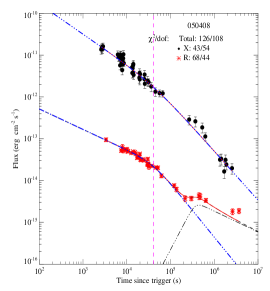
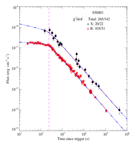
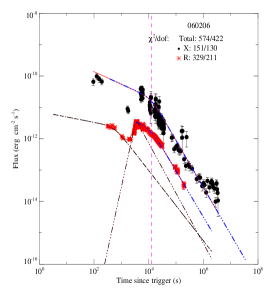
Figure 1: The X-ray and optical light curves, as well as the fitting results (blue dotted-dashed lines) for the GRBs in the Grade I sample. If an achromatic break exists, the achromatic break time is shown by a purple vertical dashed line.

Fig. 1—Continued

Fig. 1—Continued

Fig. 1—Continued

Fig. 1—Continued

Figure 2: Same as Figure 1, but for the Grade II sample

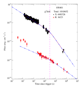
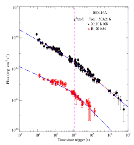
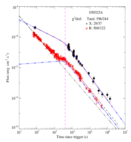
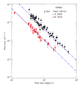
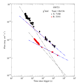
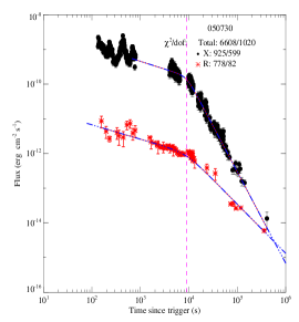
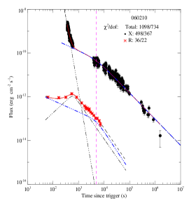
Figure 3: Same as Figure 1, but for the Grade III sample

Fig. 3—Continued

Fig. 3—Continued

Fig. 3—Continued

Figure 10: The distributions of the temporal break change $\Delta\alpha=\alpha_{2}-\alpha_{1}$ for various sub-samples in the Gold sample, and the $\Delta\alpha$ and $\alpha$ distributions of the Silver sample. Best Gaussian fits are marked with dashed curves: (a) the $\Delta\alpha$ distributions of the entire Gold sample, with $\Delta\alpha_{\rm O}=0.94\pm 0.23$ and $\Delta\alpha_{\rm X}=0.88\pm 0.28$; (b) the $\Delta\alpha$ distributions of different sub-samples in the Gold sample, with $\Delta\alpha_{\rm O}=1.05\pm 0.17$ and $\Delta\alpha_{\rm X}=1.10\pm 0.21$ for the energy injection breaks, and $\Delta\alpha_{\rm O}=0.75\pm 0.22$ and $\Delta\alpha_{\rm X}=0.75\pm 0.22$ for the jet breaks; (c) and (d) the $\Delta\alpha$ distributions for the BPL and SPL GRBs in the Silver sample, respectively. The data are dispersed.

Figure 12: The distribution of the inferred electron spectral index $p$ from various sub-samples in the Gold sample, and their best Gaussian fits (dashed lines): (a) the entire Gold sample with $p=2.33\pm 0.48$, and the sub-samples with the optical and X-ray bands constrained in the same ($p=2.58\pm 0.39$) and different ($p=2.17\pm 0.44$) spectral regimes, respectively; (b) the sub-samples with different light curve behaviors: energy injection ($p=2.34\pm 0.38$); jet break ($p=1.91\pm 0.37$); and SPL decay ($p=2.48\pm 0.47$); (c) the sub-samples with different medium types: ISM ($p=2.43\pm 0.57$) and wind ($p=2.28\pm 0.33$).

Figure 14: The distributions of the inferred energy injection parameter $q$ and their best Gaussian fits (dashed lines): the entire Gold sample ($q=0.22\pm 0.11$), the ISM sample ($q=0.20\pm 0.12$) and the wind sample ($q=0.23\pm 0.13$).

References

- Achterberg et al. (2001) Achterberg, A., Gallant, Y. A., Kirk, J. G., & Guthmann, A. W. 2001, MNRAS, 328, 393
- Band et al. (1993) Band, D., Matteson, J., Ford, L., et al. 1993, ApJ, 413, 281
- Barniol Duran (2014) Barniol Duran, R. 2014, MNRAS, 442, 3147
- Barthelmy et al. (2005) Barthelmy, S. D., Cannizzo, J. K., Gehrels, N., et al. 2005, ApJ, 635, L133
- Beloborodov (2000) Beloborodov, A. M. 2000, ApJ, 539, L25
- Berger et al. (2003) Berger, E., Kulkarni, S. R., Pooley, G., et al. 2003, Nature, 426, 154
- Bloom et al. (2001) Bloom, J. S., Frail, D. A., & Sari, R. 2001, AJ, 121, 2879
- Burrows et al. (2005) Burrows, D. N., Romano, P., Falcone, A., et al. 2005, Science, 309, 1833
- Chevalier & Li (2000) Chevalier, R. A., & Li, Z.-Y. 2000, ApJ, 536, 195
- Chincarini et al. (2007) Chincarini, G., Moretti, A., Romano, P., et al. 2007, ApJ, 671, 1903
- Costa et al. (1997) Costa, E., Frontera, F., Heise, J., et al. 1997, Nature, 387, 783
- Curran et al. (2010) Curran, P. A., Evans, P. A., de Pasquale, M., Page, M. J., & van der Horst, A. J. 2010, ApJ, 716, L135
- Dai & Lu (1998) Dai, Z. G., & Lu, T. 1998, A&A, 333, L87
- Deng et al. (2015) Deng, W., Li, H., Zhang, B., & Li, S. 2015, ApJ, submitted (arXiv:1501.07595)
- De Pasquale et al. (2009) De Pasquale, M., Evans, P., Oates, S., et al. 2009, MNRAS, 392, 153
- Ellison & Double (2002) Ellison, D. C., & Double, G. P. 2002, Astroparticle Physics, 18, 213
- Fan & Piran (2006) Fan, Y., & Piran, T. 2006, MNRAS, 369, 197
- Fan & Wei (2005) Fan, Y. Z., & Wei, D. M. 2005, MNRAS, 364, L42
- Frail et al. (1997) Frail, D. A., Kulkarni, S. R., Nicastro, L., Feroci, M., & Taylor, G. B. 1997, Nature, 389, 261
- Frail et al. (2001) Frail, D. A., Kulkarni, S. R., Sari, R., et al. 2001, ApJ, 562, L55
- Freedman & Waxman (2001) Freedman, D. L., & Waxman, E. 2001, ApJ, 547, 922
- Gao et al. (2013) Gao, H., Lei, W.-H., Zou, Y.-C., Wu, X.-F., & Zhang, B. 2013, New A Rev., 57, 141
- Gao & Mészáros (2015) Gao, H., & Mészáros, P. 2015, ApJ, in press (arXiv:1411.2650)
- Gao & Zhang (2015) Gao, H., & Zhang, B. 2015, ApJ, in press (arXiv:1409.3584)
- Gehrels et al. (2004) Gehrels, N., Chincarini, G., Giommi, P., et al. 2004, ApJ, 611, 1005
- Genet et al. (2007) Genet, F., Daigne, F., & Mochkovitch, R. 2007, MNRAS, 381, 732
- Ghisellini et al. (2007) Ghisellini, G., Ghirlanda, G., Nava, L., & Firmani, C. 2007, ApJ, 658, L75
- Granot & Kumar (2003) Granot, J., & Kumar, P. 2003, ApJ, 591, 1086
- Granot & Sari (2002) Granot, J., & Sari, R. 2002, ApJ, 568, 820
- Harrison et al. (1999) Harrison, F. A., Bloom, J. S., Frail, D. A., et al. 1999, ApJ, 523, L121
- Huang et al. (2007) Huang, K. Y., Urata, Y., Kuo, P. H., et al. 2007, ApJ, 654, L25
- Huang et al. (1999) Huang, Y. F., Dai, Z. G., & Lu, T. 1999, MNRAS, 309, 513
- Huang et al. (2000) Huang, Y. F., Gou, L. J., Dai, Z. G., & Lu, T. 2000, ApJ, 543, 90
- Ioka et al. (2005) Ioka, K., Kobayashi, S., & Zhang, B. 2005, ApJ, 631, 429
- Kaneko et al. (2006) Kaneko, Y., Preece, R. D., Briggs, M. S., et al. 2006, ApJS, 166, 298
- Kann et al. (2006) Kann, D. A., Klose, S., & Zeh, A. 2006, ApJ, 641, 993
- Kann et al. (2010) Kann, D. A., Klose, S., Zhang, B., et al. 2010, ApJ, 720, 1513
- Kann et al. (2011) —. 2011, ApJ, 734, 96
- Kobayashi & Sari (2001) Kobayashi, S., & Sari, R. 2001, ApJ, 551, 934
- Kumar (1999) Kumar, P. 1999, ApJ, 523, L113
- Kumar & Barniol Duran (2009) Kumar, P., & Barniol Duran, R. 2009, MNRAS, 400, L75
- Kumar & Barniol Duran (2010) —. 2010, MNRAS, 409, 226
- Kumar & Granot (2003) Kumar, P., & Granot, J. 2003, ApJ, 591, 1075
- Kumar et al. (2008a) Kumar, P., Narayan, R., & Johnson, J. L. 2008a, MNRAS, 388, 1729
- Kumar et al. (2008b) —. 2008b, Science, 321, 376
- Kumar & Zhang (2015) Kumar, P., & Zhang, B. 2015, Phys. Rep. 561, 1
- Lazzati et al. (2013) Lazzati, D., Morsony, B. J., Margutti, R., & Begelman, M. C. 2013, ApJ, 765, 103
- Lazzati & Perna (2007) Lazzati, D., & Perna, R. 2007, MNRAS, 375, L46
- Li et al. (2012) Li, L., Liang, E.-W., Tang, Q.-W., et al. 2012, ApJ, 758, 27
- Li et al. (2015) Li, L., Wu, X.-F., Huang, Y.-F., et al. 2015, ApJ, 805, 13
- Liang et al. (2008) Liang, E.-W., Racusin, J. L., Zhang, B., Zhang, B.-B., & Burrows, D. N. 2008, ApJ, 675, 528
- Liang et al. (2007) Liang, E.-W., Zhang, B.-B., & Zhang, B. 2007, ApJ, 670, 565
- Liang et al. (2006) Liang, E. W., Zhang, B., O’Brien, P. T., et al. 2006, ApJ, 646, 351
- Liang et al. (2013) Liang, E.-W., Li, L., Gao, H., et al. 2013, ApJ, 774, 13
- Lloyd-Ronning & Zhang (2004) Lloyd-Ronning, N. M., & Zhang, B. 2004, ApJ, 613, 477
- Lü & Zhang (2014) Lü, H.-J., & Zhang, B. 2014, ApJ, 785, 74
- Margutti et al. (2010) Margutti, R., Guidorzi, C., Chincarini, G., et al. 2010, MNRAS, 406, 2149
- Maselli et al. (2014) Maselli, A., Melandri, A., Nava, L., et al. 2014, Science, 343, 48
- Maxham & Zhang (2009) Maxham, A., & Zhang, B. 2009, ApJ, 707, 1623
- Medvedev & Loeb (1999) Medvedev, M. V., & Loeb, A. 1999, ApJ, 526, 697
- Mészáros & Rees (1997) Mészáros, P., & Rees, M. J. 1997, ApJ, 476, 232
- Mészáros et al. (1998) Mészáros, P., Rees, M. J., & Wijers, R. A. M. J. 1998, ApJ, 499, 301
- Molinari et al. (2007) Molinari, E., Vergani, S. D., Malesani, D., et al. 2007, A&A, 469, L13
- Nardini et al. (2006) Nardini, M., Ghisellini, G., Ghirlanda, G., et al. 2006, A&A, 451, 821
- Nishikawa et al. (2009) Nishikawa, K.-I., Niemiec, J., Hardee, P. E., et al. 2009, ApJ, 698, L10
- Nousek et al. (2006) Nousek, J. A., Kouveliotou, C., Grupe, D., et al. 2006, ApJ, 642, 389
- Panaitescu & Kumar (2001) Panaitescu, A., & Kumar, P. 2001, ApJ, 554, 667
- Panaitescu & Kumar (2001) —. 2001, ApJ, 554, 667
- Panaitescu & Kumar (2002) —. 2002, ApJ, 571, 779
- Panaitescu et al. (2006) Panaitescu, A., Mészáros, P., Gehrels, N., Burrows, D., & Nousek, J. 2006, MNRAS, 366, 1357
- Panaitescu et al. (1998) Panaitescu, A., Mészáros, P., & Rees, M. J. 1998, ApJ, 503, 314
- Panaitescu et al. (1999) Panaitescu, A., Spada, M., & Mészáros, P. 1999, ApJ, 522, L105
- Panaitescu & Vestrand (2008) Panaitescu, A., & Vestrand, W. T. 2008, MNRAS, 387, 497
- Panaitescu & Vestrand (2011) —. 2011, MNRAS, 414, 3537
- Perley et al. (2014) Perley, D. A., Cenko, S. B., Corsi, A., et al. 2014, ApJ, 781, 37
- Preece et al. (2000) Preece, R. D., Briggs, M. S., Mallozzi, R. S., et al. 2000, ApJS, 126, 19
- Racusin et al. (2009) Racusin, J. L., Liang, E. W., Burrows, D. N., et al. 2009, ApJ, 698, 43
- Racusin et al. (2011) Racusin, J. L., Oates, S. R., Schady, P., et al. 2011, ApJ, 738, 138
- Rees & Mészáros (1998) Rees, M. J., & Mészáros, P. 1998, ApJ, 496, L1
- Rhoads (1999) Rhoads, J. E. 1999, ApJ, 525, 737
- Rossi et al. (2002) Rossi, E., Lazzati, D., & Rees, M. J. 2002, MNRAS, 332, 945
- Sakamoto et al. (2009) Sakamoto, T., Sato, G., Barbier, L., et al. 2009, ApJ, 693, 922
- Santana et al. (2014) Santana, R., Barniol Duran, R., & Kumar, P. 2014, ApJ, 785, 29
- Sari & Esin (2001) Sari, R., & Esin, A. A. 2001, ApJ, 548, 787
- Sari & Mészáros (2000) Sari, R., & Mészáros, P. 2000, ApJ, 535, L33
- Sari et al. (1999) Sari, R., Piran, T., & Halpern, J. P. 1999, ApJ, 519, L17
- Sari et al. (1998) Sari, R., Piran, T., & Narayan, R. 1998, ApJ, 497, L17
- Schulze et al. (2011) Schulze, S., Klose, S., Björnsson, G., et al. 2011, A&A, 526, A23
- Shen et al. (2006) Shen, R., Kumar, P., & Robinson, E. L. 2006, MNRAS, 371, 1441
- Swenson et al. (2013) Swenson, C. A., Roming, P. W. A., De Pasquale, M., & Oates, S. R. 2013, ApJ, 774, 2
- Tagliaferri et al. (2005) Tagliaferri, G., Goad, M., Chincarini, G., et al. 2005, Nature, 436, 985
- Troja et al. (2007) Troja, E., Cusumano, G., O’Brien, P. T., et al. 2007, ApJ, 665, 599
- Uhm & Beloborodov (2007) Uhm, Z. L., & Beloborodov, A. M. 2007, ApJ, 665, L93
- Uhm & Zhang (2014a) Uhm, Z. L., & Zhang, B. 2014a, ApJ, 780, 82
- Uhm & Zhang (2014b) —. 2014b, ApJ, 789, 39
- Uhm & Zhang (2014c) —. 2014c, Nature Physics, 10, 351
- Uhm et al. (2012) Uhm, Z. L., Zhang, B., Hascoët, R., et al. 2012, ApJ, 761, 147
- van Eerten & Wijers (2009) van Eerten, H. J., & Wijers, R. A. M. J. 2009, MNRAS, 394, 2164
- van Paradijs et al. (1997) van Paradijs, J., Groot, P. J., Galama, T., et al. 1997, Nature, 386, 686
- Virgili et al. (2012) Virgili, F. J., Qin, Y., Zhang, B., & Liang, E. 2012, MNRAS, 424, 2821
- Wang et al. (2013) Wang, X.-G., Liang, E.-W., Li, L., et al. 2013, ApJ, 774, 132
- Waxman (1997) Waxman, E. 1997, ApJ, 485, L5
- Willingale et al. (2007) Willingale, R., O’Brien, P. T., Osborne, J. P., et al. 2007, ApJ, 662, 1093
- Wijers & Galama (1999) Wijers, R. A. M. J., & Galama, T. J. 1999, ApJ, 523, 177
- Wijers et al. (1997) Wijers, R. A. M. J., Rees, M. J., & Meszaros, P. 1997, MNRAS, 288, L51
- Wu et al. (2004) Wu, X. F., Dai, Z. G., & Liang, E. W. 2004, ApJ, 615, 359
- Yi et al. (2013) Yi, S.-X., Wu, X.-F., & Dai, Z.-G. 2013, ApJ, 776, 120
- Yost et al. (2003) Yost, S. A., Harrison, F. A., Sari, R., & Frail, D. A. 2003, ApJ, 597, 459
- Zhang et al. (2006) Zhang, B., Fan, Y. Z., Dyks, J., et al. 2006, ApJ, 642, 354
- Zhang et al. (2007a) Zhang, B., Liang, E., Page, K. L., et al. 2007a, ApJ, 655, 989
- Zhang & Mészáros (2001) Zhang, B., & Mészáros, P. 2001, ApJ, 552, L35
- Zhang & Mészáros (2002) —. 2002, ApJ, 566, 712
- Zhang & Mészáros (2004) —. 2004, International Journal of Modern Physics A, 19, 2385
- Zhang & Yan (2011) Zhang, B., & Yan, H. 2011, ApJ, 726, 90
- Zhang et al. (2007b) Zhang, B., Zhang, B.-B., Liang, E.-W. et al. 2007b, ApJ, 655, L25
- Zhang et al. (2007c) Zhang, B.-B., Liang, E.-W., & Zhang, B. 2007c, ApJ, 666, 1002
- Zhang et al. (2014) Zhang, B.-B., Zhang, B., Murase, K., Connaughton, V., & Briggs, M. S. 2014, ApJ, 787, 66
- Zhang & MacFadyen (2009) Zhang, W., & MacFadyen, A. 2009, ApJ, 698, 1261