Nanoscale fluid structure of liquid-solid-vapour

contact lines for a wide range of contact angles

A. Nold^a, D. N. Sibley ^a, B. D. Goddard ^b and S. Kalliadasis ^a

^a Department of Chemical Engineering, Imperial College London, London SW7 2AZ, UK

^b The School of Mathematics and Maxwell Institute for Mathematical Sciences

The University of Edinburgh, Edinburgh EH9 3JZ, UK

Abstract. We study the nanoscale behaviour of the density of a simple fluid in the vicinity of an equilibrium contact line for a wide range of Young contact angles $\theta_{\text{Y}}\in[40^{\circ},135^{\circ}]$. Cuts of the density profile at various positions along the contact line are presented, unravelling the apparent step-wise increase of the film height profile observed in contour plots of the density. The density profile is employed to compute the normal pressure acting on the substrate along the contact line. We observe that for the full range of contact angles, the maximal normal pressure cannot solely be predicted by the curvature of the adsorption film height, but is instead softened – likely by the width of the liquid-vapour interface. Somewhat surprisingly however, the adsorption film height profile can be predicted to a very good accuracy by the Derjaguin-Frumkin disjoining pressure obtained from planar computations, as was first shown in [Nold et al., Phys. Fluids, 26, 072001, 2014] for contact angles $\theta_{\text{Y}}<90^{\circ}$, a result which here we show to be valid for the full range of contact angles. This suggests that while two-dimensional effects cannot be neglected for the computation of the normal pressure distribution along the substrate, one-dimensional planar computations of the Derjaguin-Frumkin disjoining pressure are sufficient to accurately predict the adsorption height profile. Key words:adsorption, contact line, simple fluid, disjoining pressure, Derjaguin-Frumkin, Hamiltonian

1. Introduction

Consider a fluid interface in contact with a solid substrate. This scenario describes a container filled with liquid, a drop sitting on a leaf, or a vapour bubble inside a liquid filled bottle. Imagine observing a point in the vapour phase. As the liquid phase is approached, a rapid, yet smooth transition in the density occurs at the liquid-vapour interface. Staying on this interface and approaching the substrate, would reveal a variety of physical effects that become significant. First, the fluid feels an attractive force of the wall particles. At the same time, the nature of the solid substrate forces the fluid particles to ‘jam’ and restrict their mobility as the wall is approached.

In this work, we are interested in the effect of the wall attractive forces on the density profile in the vicinity of a three-phase contact line for a wide range of contact angles. Developing a fundamental understanding of these small-scale phenomena at equilibrium is important to predict the dynamic nanoscale behaviour of the moving contact line, which is still a controversial problem with a wide range of physical explanations being offered (for a review, see Bonn et al. [4] or Snoeijer and Andreotti [37]). In this context, our intention is twofold: First, to illustrate and give a general understanding for the density structure of the fluid as well as its form and scale of variations in the vicinity of the contact line; and second, to illustrate the impact of the contact line on the normal pressure distribution acting on the substrate. The latter point is directly connected with the definiton of the disjoining pressure. The uniqueness of disjoining pressure definitions was recently discussed critically in several papers [16, 15, 19, 14, 13, 26].

To describe the interaction between a solid substrate and a fluid interface, we choose to model a simple fluid, i.e. a system of identical particles in contact with a homogeneous, perfectly flat, hard wall. The particles of the fluid are modelled as hard spheres interacting with a Lennard-Jones type potential decaying with $r^{-6}$, where $r$ is the interparticle distance. The wall and fluid particles are assumed to interact via a similar Lennard-Jones type potential.

Contact line models, including nonlocal contributions to the free energy beyond those of the disjoining pressure, have previously been studied analytically [23, 28, 36, 12, 37]. However, for the sake of analytical attainability, only simple models of the free energy model are considered and restrictive assumptions on the nature of the density profile at the contact line are made.

In contrast, we consider the density structure at the contact line numerically employing classical density functional theory (DFT), an approach derived from the statistical mechanics of fluids [9]. DFT has proven to be a numerically efficient way to model equilibrium properties of inhomogeneous fluid systems. It can be viewed as middle ground between continuum hydrodynamics, which is inapplicable at small fluid volumes, and particle-based Monte-Carlo (MC) or Molecular Dynamics (MD) simulations, which despite dramatic improvements in computational power are still restricted to small fluid volumes. In fact, compared to MC or MD simulations, for which the numerical complexity scales with the number of particles modelled, DFT gives the ability to solve directly for the density distribution, with the advantage that its computational complexity is formally independent of the number of particles. Thus, modelling larger systems, such as contact lines, becomes feasible.

The predictive qualities of the DFT results depend on the accuracy of the free-energy model employed. Here, we model the hard-sphere free energy with a fundamental measure theory (FMT) [29], while the attractive forces are included as a Barker-Henderson perturbation [2] in a mean-field manner. DFT-FMT has been applied successfully in studies of critical point wedge filling [21], phase transitions in nanocapillaries [42], thin films on planar substrates [41] and density computations in the vicinity of liquid wedges [22]. A previous study by Pereira et al. [27] on equilibrium contact lines utilised a DFT local-density approximation (LDA) which is not appropriate to describe structuring in the fluid and fails to describe the oscillatory behavior of the density in the immediate vicinity of a wall.

The present work parallels our previous study in [26] where DFT-FMT was used to analyse the fluid structure in the immediate vicinity of a contact line for $\theta_{\text{Y}}<90^{\circ}$. Here we investigate a wide spectrum of contact angles $40^{\circ}<\theta_{\text{Y}}<135^{\circ}$ and we shed further light on the density structure in the vicinity of the contact line and its dependency on the wall strength. A discussion of the special case of a $90^{\circ}$ contact angle is also included. We present density profiles slice by slice as we sweep through the contact line region and we contrast the profiles with that of a planar liquid film on a substrate with the same film thickness, but at an off-saturation chemical potential. Interestingly, the two are not that different, which suggests that results of the planar film case may be transferable to the contact line. In particular, as in [26] we shall scrutinize the ability of Derjaguin-Frumkin theory [5] for planar liquid films on a substrate to predict the height profile at the contact line. We offer a unified Derjaguin-Frumkin treatment of the contact line for $\theta_{\text{Y}}<90^{\circ}$ and $\theta_{\text{Y}}>90^{\circ}$ by appropriately extending the boundary conditions for the disjoining pressure equation to account for the case $\theta_{\text{Y}}>90^{\circ}$. We further study the connection between the Derjaguin-Frumkin disjoining pressure and the normal pressure distribution acting on the substrate for non-planar liquid films, such as given by the contact line, for $40^{\circ}<\theta_{\text{Y}}<135^{\circ}$.

In section 2 we give an overview of the DFT model employed to solve for the equilibrium density profile. The numerical scheme to compute the contact angles is introduced in section 3. A description of the density structure in the vicinity of the contact line is given in section 4, before discussing coarse-grained Hamiltonian approaches in section 5. Finally, a general discussion of the results and concluding remarks are in section 6.

2. Statistical mechanics framework

As done for contact angles less than $90^{\circ}$ in Ref. [26], we employ classical DFT to investigate the density distribution in the vicinity of an equilibrium contact line at contact angles both greater and less than $90^{\circ}$. It is based on a statistical mechanics description and has been successfully applied in the study of inhomogeneous fluids. It is based on the theorem of Mermin [24], which allows the Helmholtz free energy $\mathcal{F}$ to be written as a unique functional of the number density $n({\bf r})$ [40]. The equilibrium density distribution minimizes the grand potential [9]

$$\Omega[n]=\mathcal{F}[n]+\int n({\bf r})\left\{V_{\text{ext}}({\bf r})-\mu\right\}\text{d}{\bf r},$$ (2.1)

where $\mu$ is the chemical potential and $V_{\text{ext}}$ is the external potential, dependent on the position vector ${\bf r}$. We then minimize Eq. (2.1) by solving the Euler-Lagrange equation

$$\frac{\delta\Omega[n]}{\delta n({{\bf r}})}=0,$$ (2.2)

where for a simple fluid of particles interacting with a Lennard-Jones potential, the free energy is usually separated into a repulsive hard-sphere part and an attractive contribution

$$\mathcal{F}[n]=\mathcal{F}_{\text{HS}}[n]+\mathcal{F}_{\text{attr}}[n].$$ (2.3)

To accurately model both the structure and thermodynamics of hard-sphere fluids, we use the Rosenfeld FMT approach [29] for the hard-sphere contribution [30]. The attractive interactions are modelled with a mean-field Barker-Henderson approach [2]

$$\mathcal{F}_{\text{attr}}[n] =\frac{1}{2}\iint\phi_{\text{attr}}({|{\bf r}-{\bf r}^{\prime}|})n({\bf r})n({\bf r}^{\prime})\text{d}{\bf r}^{\prime}\text{d}{\bf r},$$ (2.4)

where the attractive interaction potential is given by

$$\phi_{\text{attr}}\left(r\right)=\varepsilon\left\{\begin{array}[]{ll}0&\text{for }r\leq\sigma\\ 4\left(\left(\frac{\sigma}{r}\right)^{12}-\left(\frac{\sigma}{r}\right)^{6}\right)&\text{for }r>\sigma\end{array}\right..$$ (2.7)

Here, $\varepsilon$ is the depth of the Lennard-Jones potential, $\sigma$ is the distance from the center of the particle at which the Lennard-Jones potential is zero, and $r$ is a (scalar) radial distance. The simple fluid described by (2.1)–(2.7) has a critical point at $k_{B}T_{c}/\varepsilon=1.0$, where $k_{B}$ is the Boltzmann constant. Computations in this work are performed at $T=0.75T_{c}$, at which the liquid and vapour number densities are well-separated ($n_{\text{liq}}\sigma^{3}=0.622$, $n_{\text{vap}}\sigma^{3}=0.003$) and at which the liquid-vapour surface tension resulting from planar DFT computations is $\gamma_{\text{lv}}=0.3463\varepsilon/\sigma^{2}$. All two-dimensional (2D) computations are performed at the saturation chemical potential, at which the bulk vapour and bulk liquid are equally stable.

The wall-fluid particle interaction is modelled analogously to the fluid-fluid interaction as

$$\phi_{\text{attr}}^{\text{wf}}\left(r\right)=\varepsilon_{\text{w}}\left\{\begin{array}[]{ll}\infty&\text{for }r\leq\sigma\\ 4\left(\left(\frac{\sigma}{r}\right)^{12}-\left(\frac{\sigma}{r}\right)^{6}\right)&\text{for }r>\sigma\end{array}\right.,$$ (2.10)

where $\varepsilon_{\text{w}}$ is the depth of the wall-fluid interactions. Let us take a Cartesian coordinate system with the $x$-$z$ plane parallel to the wall and the $y$-coordinate in the direction normal to the wall. The external potential can then be obtained analytically from the integration of the interactions over the uniform density distribution of wall particles $n_{\text{w}}$ for $y\leq-\sigma$, giving

$$V_{\text{ext}}\left(y\right) =\left\{\begin{array}[]{ll}\infty&y\leq 0\\ \frac{2}{3}\pi\alpha_{\text{w}}\sigma^{3}\left[\frac{2}{15}\left(\frac{\sigma}{y+\sigma}\right)^{9}-\left(\frac{\sigma}{y+\sigma}\right)^{3}\right]&y>0\end{array}\right.,$$ (2.13)

where $\alpha_{\text{w}}=n_{\text{w}}\varepsilon_{\text{w}}$ is the strength of the wall potential.

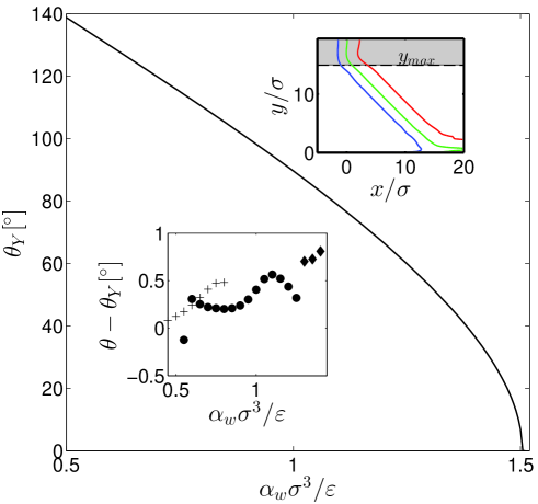
Figure 1: Plot of the Young contact angle $\theta_{\text{Y}}$ dependence on the strength of the wall attraction $\alpha_{\text{w}}$. Computations for $\gamma_{\text{lv}}$, $\gamma_{\text{wv}}$ and $\gamma_{\text{wl}}$ are done in a planar geometry, which are then inserted in (3.3). In the bottom left inset $\theta_{\text{Y}}$ is compared to 2D contact angle measurements $\theta$ which are solved for $y<y_{\text{max}}=15\sigma$ and with $\theta_{\text{n}}=90^{\circ}$ ($\bullet)$, $\theta_{\text{n}}=120^{\circ}$ ($+$) and $\theta_{\text{n}}=40^{\circ}$ ($\blacklozenge$). The top right inset depicts the contour lines of the density profile for a Cartesian grid ($\theta_{\text{n}}=90^{\circ}$) and $\alpha_{\text{w}}\sigma^{3}/\varepsilon=0.55$ (giving $\theta_{\text{Y}}=134.2^{\circ}$) for $y_{\text{max}}=15\sigma$.

3. Numerical Method

To solve (2.2) numerically in a 2D domain, we employ a spectral collocation method [38]. We have used this method successfully in our previous studies with both DFT-LDA and DFT-FMT (e.g. [42, 41, 26]). It should be emphasized that because the equations we wish to solve are non-local, the resulting matrices following discretization are dense, however the advantage of the spectral collocation method is that through a convenient choice of collocation points their number may be kept relatively low, leading to significant reduction in the size of the matrices. The reduction in the number of points becomes increasingly important when going to higher dimensions (as the number of points in a product grid scales exponentially with the dimension).

Consider the tensor product of two one-dimensional (1D) Chebychev grids on the box $(\xi,\eta)\in[-1,1]\times[-1,1]$. This computational domain is mapped onto the half space $[-\infty,\infty]\times[0,\infty]$ by

$$x^{\prime}=L_{1}\frac{\xi}{\sqrt{1-\xi^{2}}},\qquad y^{\prime}=L_{2}\frac{1+\eta}{1-\eta}.$$ (3.1)

Here, $L_{1}$ and $L_{2}$ are numerical parameters determining the spatial resolution of the collocation points close to $x^{\prime}=0$ and in the vicinity of the wall, respectively. This Cartesian grid in the physical half-space is then skewed by an angle $\theta_{n}$ using the map

$$x=\frac{x^{\prime}}{\sin\theta_{n}}+y^{\prime}\cot\theta_{n},\qquad y=y^{\prime}.$$ (3.2)

The skewed grid allows us to have more discretization points near the fluid-fluid and fluid-solid interface where higher density gradients are expected. In our computations, we assume that the liquid-vapour interface is at an angle of $\theta_{n}$ for values $y\geq y_{\text{max}}$, and only solve for collocation points located at $y<y_{\text{max}}$, such that the resulting density profiles may only be interpreted for $y<y_{\text{max}}$. In order to minimize the numerical inaccuracy caused by this cut-off, we iteratively adapt $\theta_{n}$ and increase $y_{\text{max}}$ to obtain a final result which is fully physically interpretable.

Physically, the contact angle of a liquid wedge is uniquely defined through the surface tensions of the liquid-vapour phase, $\gamma_{\text{lv}}$, and the wall-fluid pair ($\gamma_{\text{wv}}$ and $\gamma_{\text{wl}}$ being wall-vapour and wall-liquid surface tensions, respectively), given by the Young equation

$$\gamma_{\text{lv}}\cos\theta_{\text{Y}}=\gamma_{\text{wv}}-\gamma_{\text{wl}},$$ (3.3)

where the surface tensions are quantities that can be extracted from planar/(1D) DFT computations and $\theta_{\text{Y}}$ is defined as the Young contact angle. Given that we restrict our attention to systems at temperature $T/T_{c}=0.75$, the only parameter on which $\theta_{\text{Y}}$ depends is the strength of the wall attraction $\alpha_{\text{w}}$. In figure 1, we plot the dependence of $\theta_{\text{Y}}$ on the wall attraction. As expected intuitively, the contact angle decreases with increasing wall-fluid attraction and reaches complete wetting at the critical value of $\alpha_{\text{w,crit}}\sigma^{3}/\varepsilon=1.50$. In 2D computations, the contact angle of the liquid-vapour interface has to converge to $\theta_{\text{Y}}$ at large distances from the wall.

To check this, we have performed computations on a Cartesian grid, employing (3.1) and (3.2) with $\theta_{n}=90^{\circ}$, and assuming that above a limiting value $y_{\text{max}}$, the density at the collocation points corresponds to an equilibrium liquid-vapour interface with a $90^{\circ}$ contact angle. The result of the density profile for such a computation is depicted in the top right inset of figure 1. By measuring the slope of the isodensity line for $n=(n_{\text{liq}}+n_{\text{vap}})/2$ in the interval $y\in[10\sigma,14\sigma]$, we obtain an estimate for the contact angle in a 2D setting. The deviations to the $\theta_{\text{Y}}$ are shown in the bottom left inset of figure 1, showing very good agreement.

We have also performed computations on skewed grids, to increase the number of collocation points in the vicinity of the contact line and the liquid-vapour interface, by assuming that the liquid-vapour interface is at an angle of $\theta_{n}$ for values $y\geq y_{\text{max}}$. This allowed us to increase the value of $y_{\text{max}}$ to higher values. The corresponding behaviour is shown in figure 2, where for a wall attraction of $\alpha_{w}\sigma^{3}/\varepsilon=0.55$ corresponding to $\theta_{\text{Y}}=134.14^{\circ}$, the numerical parameters $y_{\text{max}}$ and $\theta_{n}$ are varied. It is seen that for all values of $y_{\max}$ and $\theta_{n}$ the contact angle approaches $\theta_{\text{Y}}$ for increasing $y$, before converging to $\theta=\theta_{n}$ near $y=y_{\max}$ due to the imposed boundary condition. For reference, the principal results presented in figure 3 were computed on a grid with $45\times 75$ collocation points and parameters $y_{\text{max}}=35\sigma$ and $\theta_{n}=\{135^{\circ},120^{\circ},90^{\circ},60^{\circ},40^{\circ}\}$ for the different rows, respectively.

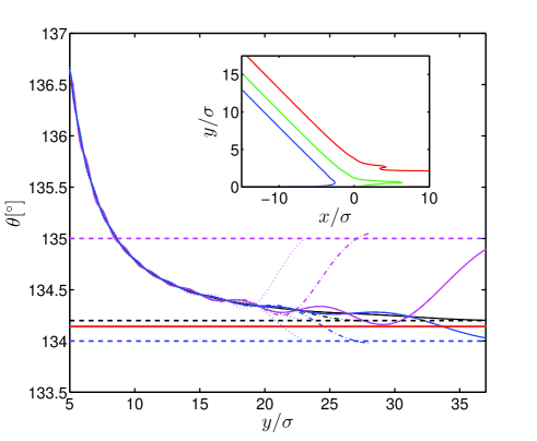
Figure 2: Slope of the isodensity line for $n=\left(n_{\text{vap}}+n_{\text{liq}}\right)/2$ for $y_{\max}=\{20,25,35\}$, represented by the dotted, dash-dotted and solid lines, respectively. Computations are done on a skewed grid with $\theta_{n}=135^{\circ}$, $134^{\circ}$ and $134.2^{\circ}$, represented by horizontal dashed lines, and results for which are drawn with magenta, blue and black lines, respectively. The substrate strength is $\alpha_{w}\sigma^{3}/\varepsilon=0.55$, leading to $\theta_{\text{Y}}=134.14^{\circ}$, depicted by the red horizontal line. The inset shows a typical contour plot for the density, where the contour lines correspond to number densities $\left(n-n_{\text{vap}}\right)/\left(n_{\text{liq}}-n_{\text{vap}}\right)=\{0.05,0.5,0.95\}$ from left to right, respectively.

4. Fluid structure in the vicinity of the contact line

Figure 3 reveals the density structure for a fluid in the vicinity of the contact line for different wall strengths. It can be seen that depending on the wall strength parameter $\alpha_{\text{w}}$, the contact density at the wall for the wall-liquid interface changes significantly. In particular, we have checked the consistency of the observed behaviour with the wall-fluid virial equation [16]

$$p=-\int_{-\infty}^{\infty}n(y)V^{\prime}_{\text{ext}}(y)\text{d}y=n(0)-\int_{0}^{\infty}n(y)V^{\prime}_{\text{ext}}(y)\text{d}y,$$ (4.1)

where $n(0)$ stems from the delta-function contribution to $V^{\prime}_{\text{ext}}$ at $y=0$.

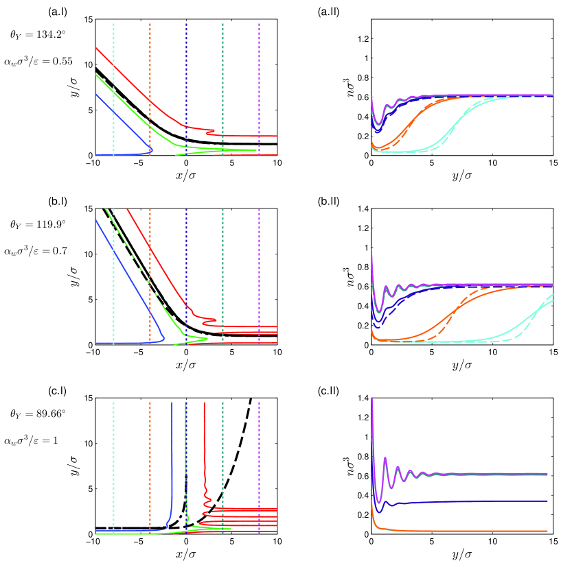
For caption, see next page.

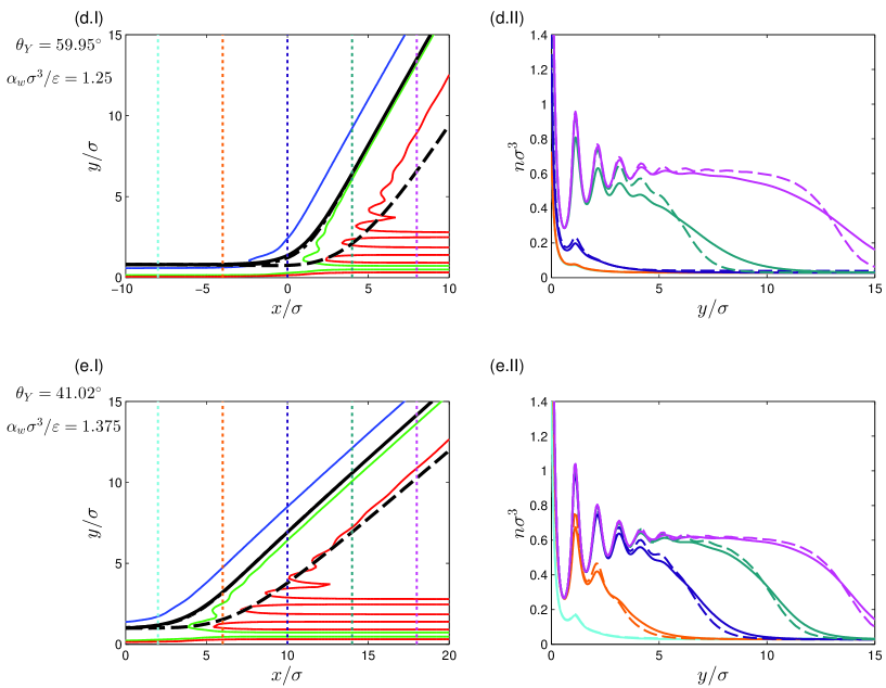
Figure 3: Contour lines for the number density (left column, subfigures I) and density profiles as a function of the distance to the substrate at various positions $x$ along the substrate (right column, subfigures II). In the left column, the contour lines correspond to number densities $\left(n-n_{\text{vap}}\right)/\left(n_{\text{liq}}-n_{\text{vap}}\right)=\{0.05,0.5,0.95\}$ from left to right. The height profiles $h_{\text{I,II,III}}$, defined through equation (5.8) with boundary conditions (5.9)-(5.10) and equation (5.15), are depicted by black dash-dotted, dashed and solid lines, respectively, $h_{\text{I}}$ being virtually indistinguishable from $h_{\text{III}}$. The solid lines in the right column represent the 2D density profile, plotted along the dashed vertical lines of corresponding colour in the left column figures. These density profiles are compared to the equivalent planar off-saturation liquid or vapour film of the same adsorption film thickness, drawn with dashed lines.

The density plots at different positions in $x$ across the contact line in the right column of figure 3 provide an insight as to how the transition between a wall-vapour and a wall-liquid interface leads to a quasi step-like increase of the density in the contour plots. We note that this transition is accompanied by a gradual increase of the distance between the liquid-vapour interface and the wall. A similar transition can be observed when gradually varying the chemical potential for a fluid film in contact with a planar wall. A typical example of the bifurcation diagram, also widely denoted as the adsorption isotherm, representing this transition, is shown in figure 4, where the film thickness $\ell$ of the liquid or vapour film, defined by

$$\ell{\mathrel{\mathop{:}}=} \frac{1}{\Delta n}\int_{0}^{\infty}|n(\infty)-n(y)|\text{d}y$$ (4.2)

$$\qquad\text{with}\qquad\Delta n= n_{\text{liq}}-n_{\text{vap}},$$ (4.3)

is plotted versus the deviation of the chemical potential from its saturation value $\Delta\mu$. In particular, figure 4 shows the behaviour for a dewetting scenario of a growing vapour film. Each point on the adsorption isotherm represents a density profile which satisfies the Euler-Lagrange equation (2.2) for a planar configuration. As saturation is approached, the adsorption isotherm satisfies the expected inverse cubic decay of $\Delta\mu$ with $\ell$ for systems with dispersion forces [8], such as shown in the inset of figure 4.

These density profiles are compared in the right column of figure 3 with density profiles across the contact line which have the same adsorption (4.2). We note that the contact line is computed at saturation chemical potential, whereas the chemical potential for the density profiles of the adsorption isotherm is naturally off-saturation. Nevertheless, the result is unexpected and shows a surprisingly good agreement, where for large film thicknesses, the density profiles at the liquid-vapour interfaces differ because for a contact line the liquid-vapour interface is at an angle to the wall, while the dashed lines always describe planar films.

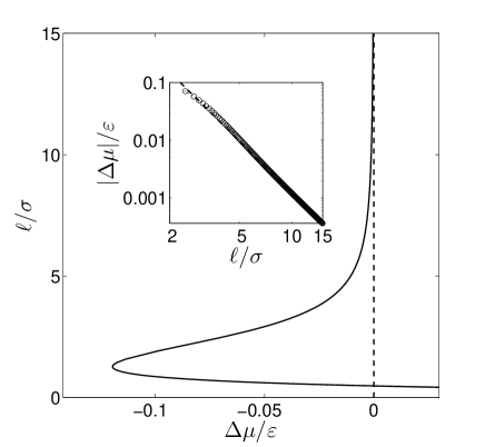
Figure 4: Plot of the adsorption isotherm for a dewetting scenario with wall attraction of $\alpha_{\text{w}}\sigma^{3}/\varepsilon=0.7$, corresponding to $\theta_{\text{Y}}=119.9^{\circ}$. The inset shows the asymptotic behaviour for large $\ell$, as $\Delta\mu\sim\ell^{-3}$, where the dashed line is a fit for $\ell\in[10\sigma,15\sigma]$ to $\Delta\mu=a\ell^{-3}$, with computed coefficient $a=-1.21\varepsilon\sigma^{3}$. In the inset individual DFT computations of the equilibrium density are marked with circles and are connected by the solid line in the main plot for clarity.

5. Hamiltonian approaches, Derjaguin-Frumkin route and disjoining pressure

In a coarse-grained description of the contact line, the two-dimensional density profile is reduced to a height profile $h(x)$ representing the liquid-vapour interface [17, 25]. At equilibrium, this height profile minimizes the Hamiltonian [16]

$$H[h]=\int_{-\infty}^{\infty}\left\{\gamma_{\text{lv}}\left(\sqrt{1+(h^{\prime})^{2}}-1\right)+V(h)\right\}\text{d}x,$$ (5.1)

where $h^{\prime}={\text{d}h}/{\text{d}x}$ is the slope of the interface and $V(h)$ is the effective interface potential. The first term in (5.1) accounts for the excess energy stored through the surface tension due to the curvature of the liquid-vapour interface, while the second term accounts for corrections to the Hamiltonian due to the presence of the substrate. This not only includes direct attractive forces between fluid and wall particles, but also corrections due to the distorted fluid density profile caused by the presence of the wall. The effective interface potential $V$ is linked to the disjoining pressure $\Pi$ by

$$\Pi\left(h\right){\mathrel{\mathop{:}}=}-\frac{\text{d}V}{\text{d}h}.$$ (5.2)

Usually, (5.1) is only applied in the lubrication approximation. For larger slopes, both the separate inclusion of the effective surface potential and surface energy [28] as well as the functional dependence of $V$ on $h$ alone, as opposed to a functional dependence on $h(x)$, were put into question [15, 19, 14, 13]. Here, we test for different disjoining pressure definitions whether (5.1) may be used to to define height profiles for a large range of contact angles.

In [26] we have compared height profiles resulting from minimizing (5.1) with two different definitions of the disjoining pressure for contact angles $\theta<90^{\circ}$. We note that these disjoining pressure definitions are different from phenomenological analytical models such as used e.g. in [34, 35] in that they are obtained directly from DFT computations, and therefore include the full information of hard-sphere as well as the attractive particle interactions. The first disjoining pressure definition we consider is based on the celebrated Derjaguin and Frumkin theory [7, 11]:

$$\Pi_{\text{I}}\left(\ell\right){\mathrel{\mathop{:}}=}-\Delta\mu\Delta n\times\left\{\begin{array}[]{ll}1&\text{for }n|_{y=\infty}=n_{\text{vap}}\\ -1&\text{for }n|_{y=\infty}=n_{\text{liq}}\end{array}\right.,$$ (5.5)

for a system at saturation chemical potential $\mu_{\text{sat}}$, and where

$$\Delta\mu =\mu_{\text{eq}}\left(\ell\right)-\mu_{\text{sat}}.$$ (5.6)

$\mu_{\text{eq}}$ is the chemical potential at which a film of thickness $\ell$ is at equilibrium, such as depicted in the adsorption isotherm in figure 4.

The first case of (5.5), $n|_{y=\infty}=n_{\text{vap}}$, describes a wetting scenario where the density at infinite distance from the wall corresponds to the equilibrium vapour density. In this case, a liquid film will slowly build as the chemical potential reaches its saturation value. In contrast, the dewetting case $n|_{y=\infty}=n_{\text{liq}}$ describes a vapour film in a bulk liquid environment, as studied in figure 4. The sign switch in (5.5) originates from the sign difference between the density in the film vs. the bulk density. We note that contact lines with contact angle $\theta_{\text{Y}}>90^{\circ}$ are described by a vapour film of varying height, whereas contact lines with contact angle $\theta_{\text{Y}}<90^{\circ}$ are described by a liquid film of varying height.

As an alternative to the Derjaguin and Frumkin definition of the disjoining pressure (5.5), one can define the disjoining pressure based on the normal force balance at the substrate. The disjoining pressure is then defined as the excess pressure acting on the substrate due to the deviation from the equilibrium density profile, caused e.g. by the boundary conditions imposed on the system [16, 15]

$$\Pi_{\text{II}}\left(x\right){\mathrel{\mathop{:}}=}-\int_{-\infty}^{\infty}\left(n(x,y)-n(\infty,y)\right)V_{\text{ext}}^{\prime}(y)\text{d}y.$$ (5.7)

Note that $n(x,y)V_{\text{ext}}^{\prime}(y)$ is the force acting through the external potential—representing the wall—on the fluid element at point $(x,y)$. In our case, $n(x,y)$ is the density profile originating from a 2D DFT computation of the contact line, and hence $\Pi_{\text{II}}$ is a quantity containing information of the full 2D equilibrium density profile; in contrast (5.5) is derived from planar 1D computations.

The equilibrium height profiles $h_{\text{I}}$ and $h_{\text{II}}$ corresponding to the disjoining pressures $\Pi_{\text{I}}$ and $\Pi_{\text{II}}$, respectively, are obtained by minimizing the Hamiltonian (5.1), leading to the defining equation for $h_{\text{I/II}}$

$$-\Pi_{\text{I}/\text{II}}=\gamma_{\text{lv}}\frac{\text{d}}{\text{d}x}\left(\frac{h_{\text{I}/\text{II}}^{\prime}}{\sqrt{1+(h_{\text{I}/\text{II}}^{\prime})^{2}}}\right),$$ (5.8)

with boundary conditions

$$\lim_{x\to-\infty}h_{\text{I}}=h_{0}\qquad\text{for }\theta_{\text{Y}}<90^{\circ},$$ (5.9)

and

$$\lim_{x\to\infty}h_{\text{I}}=h_{0}\qquad\text{for }\theta_{\text{Y}}>90^{\circ},$$ (5.10)

where $h_{0}$ is the film thickness representing the wall-vapour interface in the wetting case and the wall-liquid interface in the drying case. We note that $h_{0}$ corresponds to the (finite) value at $\Delta\mu=0$ of the adsorption isotherm in figure 4. Given that $\Pi_{\text{I}}$ is a function of $h$, and not of $x$ directly, (5.8) for $h_{\text{I}}$ is an autonomous ordinary differential equation. This means that with (5.9), (5.10) $h_{\text{I}}$ is translationally invariant in $x$. For simplicity, in figures 3 and 5, we depict one representative plot for $h_{\text{I}}$ or $\Pi_{\text{I}}(h_{\text{I}})$.

The ordinary differential equation (5.8) defining the film heights $h_{\text{I/II}}$ can also be interpreted as a form of the Young-Laplace equation for a pressure jump across a fluid interface, where the left hand side describes the difference between the pressure acting on the substrate and the fluid pressure at $y=\infty$, while the right hand side represents the product of the surface tension with the curvature of the interface.

Integrating (5.8) with respect to $x$ and $h$, respectively, leads to the normal-force balance of Young’s equation

$$-\int_{-\infty}^{\infty}\Pi_{\text{I}/\text{II}}(x)\text{d}x=\gamma_{\text{lv}}\sin\theta_{\text{Y},\text{I}/\text{II}},$$ (5.11)

and the important expression of Derjaguin-Frumkin theory [6, 34]

$$-\int_{h_{0}}^{\infty}\Pi_{\text{I}/\text{II}}\left(h\right)\text{d}h=\gamma_{\text{lv}}\left(1-|\cos\theta_{\text{Y},\text{I}/\text{II}}|\right),$$ (5.12)

where $\theta_{\text{Y},\text{I}/\text{II}}\in[0,180^{\circ}]$ corresponds to the limiting slope of the height profiles $h_{\text{I,II}}$, respectively, at distances far away from the wall:

$$\theta_{\text{Y},\text{I}/\text{II}}=\lim_{h_{\text{I/II}}\to\infty}\tan^{-1}\left(h^{\prime}_{\text{I/II}}(x)\right).$$ (5.13)

Equation (5.12) can be interpreted as a force balance in direction parallel to the substrate. For $\theta_{\text{Y}}<90^{\circ}$, the right hand side of the equation represents the forces of the liquid-vapour interface acting in the negative $x$-direction. For $\theta_{\text{Y}}>90^{\circ}$, the height profile decreases from $\infty$ to $h_{0}$ as $x$ increases. Due to this inversion of the height profile, (5.12) represents the force balance in the positive $x$-direction. The force of the liquid-vapour interface acting in the positive $x$-direction is $\gamma_{\text{lv}}$, whereas the force acting in the negative direction is $\gamma_{\text{lv}}|\cos\theta_{\text{Y}}|$. We note that here, the modulus accounts for the fact that for $\theta_{\text{Y}}>90^{\circ}$, $\cos\theta_{\text{Y}}<0$, given that we have defined $\theta_{\text{Y},\text{I}/\text{II}}\in[0,180^{\circ}]$, as opposed to allowing for negative values of $\theta_{\text{Y,I/II}}$ in (5.13).

Since both sum rules are derived from (5.8), $\theta_{\text{Y},\text{I}/\text{II}}$ in equations (5.11) and (5.12) are equivalent and ultimately, both height profiles converge to the slope dictated by the Young contact angle. Thus $\theta_{\text{Y},\text{I}/\text{II}}$ both correspond to $\theta_{\text{Y}}$ defined in the Young equation (3.3). We will exploit this property to estimate the accuracy of our numerical method.

$\alpha_{w}\sigma^{3}/\varepsilon$	$\theta_{\text{Y}}$	$-\int_{h_{0}}^{\infty}\Pi_{\text{I}}\left(h\right)\text{d}h$	$\theta_{\text{Y,I}}$	$-\int_{-\infty}^{\infty}\Pi_{\text{II}}\left(x\right)\text{d}x$	$\theta_{\text{Y,II}}$
$0.55$	$134.2^{\circ}\pm 0.1^{\circ}$	$0.103\pm 0.002$	$134.5^{\circ}\pm 0.4^{\circ}$	$-0.244\pm 0.005$	$135.2^{\circ}\pm 1.1^{\circ}$
$0.7$	$119.9^{\circ}\pm 0.05^{\circ}$	$0.172\pm 0.003$	$120.3^{\circ}\pm 0.5^{\circ}$	$-0.298\pm 0.002$	$120.5^{\circ}\pm 0.7^{\circ}$
$1.0$	$89.6^{\circ}\pm 0.1^{\circ}$	$0.345\pm 0.001$	$89.8^{\circ}\pm 0.2^{\circ}$	$-0.3463\pm 10^{-4}$	($\star$)
$1.25$	$59.9^{\circ}\pm 0.1^{\circ}$	$0.173\pm 0.001$	$60.0^{\circ}\pm 0.2^{\circ}$	$-0.297\pm 0.003$	$59.1^{\circ}\pm 0.8^{\circ}$
$1.375$	$41.0^{\circ}\pm 0.1^{\circ}$	$0.085\pm 0.001$	$41.1^{\circ}\pm 0.2^{\circ}$	$-0.234\pm 0.007$	$42.5^{\circ}\pm 1.6^{\circ}$

Table 1: Comparison of $\theta_{\text{Y}}$ as defined in (3.3), the contact angles $\theta_{\text{I,II}}$ defined through (5.13) as well as the absolute errors of the integrals on the left hand sides of equations (5.11) and (5.12), respectively. ($\star$): Here, the integral expression gives $\sin\theta_{\text{Y,II}}=1.0001\pm 0.0001$, such that an estimate for $\theta_{\text{Y,II}}$ cannot formally be given.

In table 1, numerical values for the integrals of the disjoining pressures are given. Error bounds $\Delta$ are estimated by comparing the integral expressions with $\gamma_{\text{lv}}\sin\theta_{\text{Y}}$ and $\gamma_{\text{lv}}\left(1-|\cos\theta_{\text{Y}}|\right)$, respectively. These error bounds are then used to estimate error bounds of $\theta_{\text{Y,I/II}}$ by

$$\Delta\theta_{\text{Y,II}}=\left|\frac{\Delta\left\{-\int_{-\infty}^{\infty}\Pi_{\text{II}}(x)\text{d}x\right\}}{\gamma_{\text{lv}}\cos\theta_{\text{Y},\text{II}}}\right|\qquad\text{and}\qquad\Delta\theta_{\text{Y,I}}=\left|\frac{\Delta\left\{-\int_{h_{0}}^{\infty}\Pi_{\text{I}}\left(h\right)\text{d}h\right\}}{\gamma_{\text{lv}}\sin\theta_{\text{Y},\text{I}}}\right|.$$ (5.14)

The above formulations can be derived from (5.11) and (5.12) by using $\theta_{\text{Y},\text{I/II}}+\Delta\theta_{\text{Y},\text{I/II}}$ and linearly expanding to first order in $\Delta\theta_{\text{Y},\text{I/II}}$ the right hand side of the respective equation around $\theta_{\text{Y},\text{I/II}}$. Finally, we compare the film height profiles $h_{\text{I}}$ and $h_{\text{II}}$ with the adsorption film thickness

$$h_{\text{III}}(x){\mathrel{\mathop{:}}=}\frac{1}{\Delta n}\int_{0}^{\infty}|\left(n(x,y)-n(x,\infty)\right)|\text{d}y,$$ (5.15)

which is the 2D generalisation of (4.2). This allows us to define a disjoining pressure suggested by the adsorption film height, obtained by inserting $h_{\text{III}}$ into (5.8), giving the rescaled curvature

$$-\Pi_{\text{III}}(h){\mathrel{\mathop{:}}=}\gamma_{\text{lv}}\frac{\text{d}}{\text{d}x}\left(\frac{h_{\text{III}}^{\prime}}{\sqrt{1+(h_{\text{III}}^{\prime})^{2}}}\right).$$ (5.16)

In figure 3, we compare the height profiles $h_{\text{I}-\text{III}}$ in the vicinity of the contact line for a wide range of wall attractions.

6. Discussion and conclusion

We have scrutinized the fluid structure and its properties in the vicinity of a three-phase contact line by employing a DFT-FMT model. In particular, we presented density profiles slice by slice as we sweep through the contact line region and we contrast the density profiles with the profile of a planar liquid film on a substrate, but with the same film thickness, demonstrating that the two are quite similar. We also scrutinized the ability of Derjaguin-Frumkin theory [5] for planar liquid films on a substrate to predict the height profile at the contact line and we offered a unified Derjaguin-Frumkin treatment of the contact line for $\theta_{\text{Y}}<90^{\circ}$ and $\theta_{\text{Y}}>90^{\circ}$ by appropriately extending the boundary conditions for the disjoining pressure equation to account for the case $\theta_{\text{Y}}>90^{\circ}$.

In figure 3 we plot the height profiles $h_{\text{I/II/III}}$ for contact angles in the region $40^{\circ}<\theta_{\text{Y}}<135^{\circ}$ and compare them with the contour lines of the density. The figure summarizes some of the main results of our study as far as the behaviour close to the contact line is concerned. Additional information on this can be extracted from figure 5 where we compare the disjoining pressure profiles $\Pi_{\text{I/II/III}}$. An observation we made in our previous study in [26] for contact angles $\theta_{\text{Y}}<90^{\circ}$, was that the location of maximal curvature for the height profile $h_{\text{II}}$ is shifted towards the fluid phase if compared with the adsorption height profile $h_{\text{III}}$. This observation can also be made in figures 3 (g,i) and in figure 5 (b). However, this does not occur to the same extent in cases where $\theta_{\text{Y}}>90^{\circ}$—such as observed in figures 3 (a,c) and in figure 5 (a).

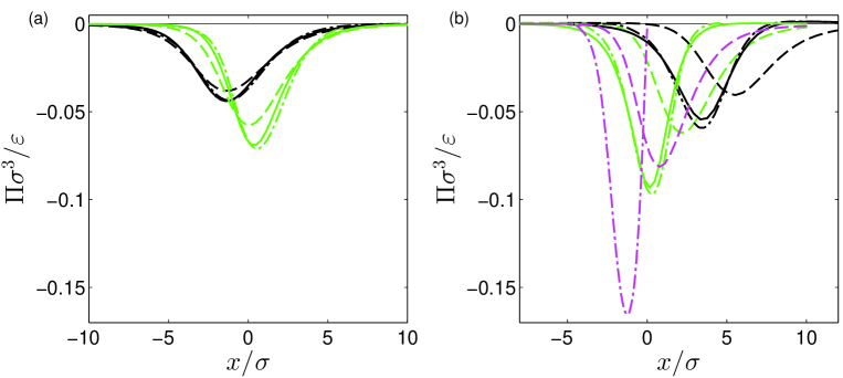
Figure 5: Plots of different disjoining pressure definitions for different wall attractions. Dash-dotted, dashed and solid lines depict disjoining pressures $\Pi_{\text{I}}$, $\Pi_{\text{II}}$ and $\Pi_{\text{III}}$, respectively. In subfigure (a), the black and green lines show data for $\alpha_{w}\sigma^{3}/\varepsilon=0.55$ and $0.7$, respectively, whilst in (b), the black, green and magenta lines show data for $\alpha_{w}\sigma^{3}/\varepsilon=1.375,1.25$ and $1.0$, respectively.

Furthermore, the maximal absolute curvature of the height profile $h_{\text{II}}$ (see dashed lines in figures 3 and 5) is lower than the maximal absolute curvature of the adsorption film height $h_{\text{III}}$ (see solid lines in figures 3 and 5). This can best be seen in figure 5 (we note that the disjoining pressure corresponds to the rescaled curvature of the corresponding height profile). While the difference is less pronounced for large contact angles $\theta_{\text{Y}}>90^{\circ}$, it is still observable. In contrast, the film thickness $h_{\text{I}}$ (see dash-dotted lines in figures 3 and 5) based on the adsorption isotherm, agrees very well with $h_{\text{III}}$, often to the point of being virtually indistinguishable (compare the left column of figure 3).

For a varying height profile, here enforced by the boundary conditions, we have studied two conflicting definitions of the disjoining pressure—one based on the adsorption isotherm, the other based on the normal force balance. These two definitions lead to distinct height profiles, which suggest that the use of the disjoining pressure based on the adsorption isotherm is more appropriate, given the good agreement of the corresponding height profile with the adsorption height profile. This is somewhat surprising, given that the disjoining pressure based on the normal force balance $\Pi_{\text{II}}$ contains information from the full equilibrium 2D density profile, whereas $\Pi_{\text{I}}$ is derived from purely 1D computations.

At the same time the behaviour of $\Pi_{\text{II}}$ is such that the maximum absolute normal pressure acting on the substrate is lower than the curvature of the adsorption height profile would suggest. Also, for $\theta_{\text{Y}}<90^{\circ}$, the maximal normal pressure does not act in the vicinity of the contact line, but instead at a slightly shifted position towards the liquid phase. This interpretation could be of interest for the nanoscale behaviour of contact lines at soft substrates, such as considered e.g. by Lubbers et al. [18].

The special case of $\theta_{\text{Y}}$ being very close to $90^{\circ}$, such as depicted in figure 3 (e,f) for $\alpha_{w}\sigma^{3}/\varepsilon=1.0$, as well as the magenta lines in figure 5 (b), deserves a comment. In this case, the density at very large distances from the wall $n|_{y\to\infty}$ depends on the position $x$, and hence does not allow for the definition of an adsorption height profile $h_{\text{III}}$ through (5.15). While the disjoining pressure $\Pi_{\text{I}}$ based on the adsorption isotherm has a very high absolute maximum, the absolute maximum of $\Pi_{\text{II}}$ is less pronounced. Also, the width of $\Pi_{\text{II}}$ corresponds roughly to the width of the interface and is slightly shifted towards the fluid phase.

An important observation, therefore, is that the maximal normal pressure acting on the substrate does not correspond with the maximal curvature of the adsorption film thickness or the maximal value of the Derjaguin-Frumkin disjoining pressure $\Pi_{\text{I}}$. One reason for the softening of the normal pressure profile could be the width of the fluid interface. In particular, one can observe in figure 5 (b), that the width of $\Pi_{\text{II}}$ for $\theta_{\text{Y}}\approx 90^{\circ}$, denoted by the dashed magenta line, corresponds approximately with the width of the liquid-vapour interface.

It is noteworthy that the main limitation of the model is that its mean-field nature does not include the description of thermal fluctuations [1, 10, 20]. Inclusion of thermal fluctuations, which become more pronounced with increasing film thicknesses $\ell$, leads to a broadening of the liquid-vapour interface and a renormalization of the dependence of $\ell$ on the chemical potential deviation from saturation $\Delta\mu$ [1] is needed. A detailed recent study based on molecular simulations and experiments has found that thermal fluctuations lead to an effective film-height dependent surface tension $\gamma_{\text{lv}}(\ell)$ in (5.1) [20]. A final conclusion about the effect on thermal fluctuations for the results presented here could be reached by a molecular simulations study in the spirit of Herring and Henderson’s analysis [16], but including dispersion forces and a comparison with the corresponding Derjaguin-Frumkin disjoining pressure. This, however, is beyond the scope of the present study.

The important observation made here is that in a mean-field model, disjoining pressures obtained from planar films via the Derjaguin-Frumkin route do allow us to predict with good accuracy the structure of the contact line, hence implying a negligeble contribution of non-locality. It would be interesting to see if this holds for other settings, e.g. spherical droplets.

Of particular interest would also be to investigate very large contact angles close to $180^{\circ}$, given interesting recent results in this case [3] as well as the influence of surface roughness and chemical heterogeneities which are known to influence wetting phenomena substantially (e.g. [31, 32, 33, 39]). We shall address these and related issues in future studies.

References

- [1] A. J. Archer, R. Evans. Relationship between local molecular field theory and density functional theory for non-uniform liquids. J. Chem. Phys., 138 (1) (2013), 014502.
- [2] J. A. Barker, D. Henderson. Perturbation theory and equation of state for fluids. II. A successful theory of liquids. J. Chem. Phys., 47 (11) (1967), 4714–4721.
- [3] E. S. Benilov, M. Vynnycky. Contact lines with a contact angle. J. Fluid Mech., 718 (2013), 481–506.
- [4] D. Bonn, J. Eggers, J. Indekeu, J. Meunier, E. Rolley. Wetting and spreading. Rev. Mod. Phys., 81 (2009), 739–805.
- [5] B. V. Derjaguin. Some results from 50 years’ research on surface forces. In Surface Forces and Surfactant Systems, volume 74 of Progress in Colloid & Polymer Science, Steinkopff, (1987), 17–30.
- [6] B. V. Derjaguin, N. V. Churaev. Properties of water layers adjacent to interfaces. In Clive A. Croxton, editor, Fluid interfacial phenomena, Wiley, New York, (1986), 663–738.
- [7] B. V. Derjaguin, E. Obuchov. Anomalien dünner Flüssigkeitsschichten. III. Acta Physicochim. URSS, 5 (1) (1936), 1-22.
- [8] S. Dietrich, M. Napiórkowski. Analytic results for wetting transitions in the presence of van der Waals tails. Phys. Rev. A, 43 (1991), 1861–1885.
- [9] R. Evans. The nature of the liquid-vapour interface and other topics in the statistical mechanics of non-uniform, classical fluids. Adv. Phys., 28 (2) (1979), 143–200.
- [10] R. Evans, J. R. Henderson, D. C. Hoyle, A. O. Parry, Z. A. Sabeur. Asymptotic decay of liquid structure: oscillatory liquid-vapour density profiles and the Fisher-Widom line. Mol. Phys., 80 (4) (1993), 755–775.
- [11] A. N. Frumkin. Über die Erscheinungen der Benetzung und des Anhaftens von Bläschen. I. Acta Physicochim. URSS, 9 (313), (1938).
- [12] T. Getta, S. Dietrich. Line tension between fluid phases and a substrate. Phys. Rev. E, 57 (1) (1998), 655–671.
- [13] J. R. Henderson. Discussion notes: Note continuing the discussion on the contact line problem. Eur. Phys. J. Special Topics, 197 (1) (2011), 129–130.
- [14] J. R. Henderson. Discussion notes on “Computer simulation of interface potentials: Towards a first principle description of complex interfaces?”, by L. G. MacDowell. Eur. Phys. J. Special Topics, 197 (1) (2011), 147–148.
- [15] J. R. Henderson. Disjoining pressure of planar adsorbed films. Eur. Phys. J. Special Topics, 197 (1) (2011), 115–124.
- [16] A. R. Herring, J. R. Henderson. Simulation study of the disjoining pressure profile through a three-phase contact line. J. Chem. Phys., 132 (8) (2010) 084702.
- [17] R. Lipowsky, M. E. Fisher. Scaling regimes and functional renormalization for wetting transitions. Phys. Rev. B, 36 (4) (1987) 2126–2141.
- [18] L. A. Lubbers, J. H. Weijs, L. Botto, S. Das, B. Andreotti, J. H. Snoeijer. Drops on soft solids: free energy and double transition of contact angles. J. Fluid Mech., (2014), 747, R1.
- [19] L. G. MacDowell. Discussion notes on “Disjoining pressure of planar adsorbed films”, by J.R. Henderson. Eur. Phys. J. Special Topics, 197 (1) (2011),149–150.
- [20] L. G. MacDowell, J. Benet, N. A. Katcho, J. M. G. Palanco. Disjoining pressure and the film-height-dependent surface tension of thin liquid films: New insight from capillary wave fluctuations. Adv. Colloid Interface Sci., 206 (2014), 150–171.
- [21] A. Malijevský, A. O. Parry. Critical point wedge filling. Phys. Rev. Lett., 110 (16) (2012), 166101.
- [22] R.-J. C. Merath. Microscopic calculation of line tensions. PhD thesis, Universität Stuttgart, 2008.
- [23] G. J. Merchant, J. B . Keller. Contact angles. Phys. Fluids A, 4 (3) (1992), 477–485.
- [24] N. D. Mermin. Thermal properties of the inhomogeneous electron gas. Phys. Rev., 137 (5A) (1965), A1441–A1443.
- [25] L. V. Mikheev, J. D. Weeks. Sum rules for interface Hamiltonians. Physica A, 177 (1) (1991), 495–504.
- [26] A. Nold, D. N. Sibley, B. D. Goddard, S. Kalliadasis. Fluid structure in the immediate vicinity of an equilibrium three-phase contact line and assessment of disjoining pressure models using density functional theory. Phys. Fluids, 26 (7) (2014) 072001.
- [27] A. Pereira, S. Kalliadasis. Equilibrium gas-liquid-solid contact angle from density-functional theory. J. Fluid Mech., 692 (2012), 53–77.
- [28] L. M. Pismen. Nonlocal diffuse interface theory of thin films and the moving contact line. Phys. Rev. E, 64 (2) (2001), 021603.
- [29] Y. Rosenfeld. Free-energy model for the inhomogeneous hard-sphere fluid mixture and density-functional theory of freezing. Phys. Rev. Lett., 63 (9) (1989), 980–983.
- [30] R. Roth. Fundamental measure theory for hard-sphere mixtures: a review. J. Phys.: Condens. Matter, 22 (6) (2010) 063102.
- [31] N. Savva, S. Kalliadasis. Two-dimensional droplet spreading over topographical substrates. Phys. Fluids, 21 (9) (2009), 092102.
- [32] N. Savva, S. Kalliadasis. Dynamics of moving contact lines: A comparison between slip and precursor film models. Europhys. Lett., 94 (6) (2011), 64004.
- [33] N. Savva, S. Kalliadasis, G. A. Pavliotis. Two-dimensional droplet spreading over random topographical substrates. Phys. Rev. Lett., 104 (8) (2010), 084501.
- [34] L. W. Schwartz. Hysteretic effects in droplet motions on heterogeneous substrates: Direct numerical simulation. Langmuir, 14 (12) (1998), 3440–3453.
- [35] D. N. Sibley, A. Nold, N. Savva, S. Kalliadasis. A comparison of slip, disjoining pressure, and interface formation models for contact line motion through asymptotic analysis of thin two-dimensional droplet spreading. J. Eng. Math., DOI: 10.1007/s10665-014-9702-9, 2014.
- [36] J. H. Snoeijer, B. Andreotti. A microscopic view on contact angle selection. Phys. Fluids, 20 (5) (2008), 057101.
- [37] J. H. Snoeijer, B. Andreotti. Moving contact lines: Scales, regimes, and dynamical transitions. Annu. Rev. Fluid Mech., 45 (2013), 269–292.
- [38] N. L. Trefethen. Spectral Methods in MATLAB. Vol. 10, SIAM, Philadelphia, 2000.
- [39] R. Vellingiri, N. Savva, S. Kalliadasis. Droplet spreading on chemically heterogeneous substrates. Phys. Rev. E, 84 (3) (2011), 036305.
- [40] J. Wu. Density functional theory for chemical engineering: From capillarity to soft materials. AIChE J., 52 (3) (2006), 1169–1193.
- [41] P. Yatsyshin, N. Savva, S. Kalliadasis. Spectral methods for the equations of classical density-functional theory: Relaxational dynamics of microscopic films. J. Chem. Phys., 136 (12) (2012), 124113.
- [42] P. Yatsyshin, N. Savva, S. Kalliadasis. Geometry-induced phase transition in fluids: Capillary prewetting. Phys. Rev. E, 87 (2) (2013), 020402(R).