Determining pressure-temperature phase diagrams of materials

Abstract

We extend the nested sampling algorithm to simulate materials under periodic boundary and constant pressure conditions, and show how it can be used to determine the complete equilibrium phase diagram, for a given potential energy function, efficiently and in a highly automated fashion. The only inputs required are the composition and the desired pressure and temperature ranges, in particular, solid-solid phase transitions are recovered without any a priori knowledge about the structure of solid phases. We benchmark and showcase the algorithm on the periodic Lennard-Jones system, aluminium and NiTi.

I Introduction

Phase diagrams of materials describe the regions of stability and equilibria of structurally distinct phases and are fundamental in both materials science and industry. In order to augment experiments, computer simulations and theoretical calculations are often used to provide reference data and describe phase transitions. A plethora of methods exist to determine individual phase boundaries, including Gibbs ensemble Monte Carlo Panagiotopoulos (1987), Gibbs–Duhem integration Kofke (1993a), thermodynamic integration and even direct molecular dynamics simulations of coexistence. Each of these algorithms requires the user to specify at least the identity and approximate location of the phase transition under investigation. Moreover, in the case of the solid phases, where much of the interest lies, advance knowledge of the crystal structure of each phase is required. Calculating an entire phase diagram by combining the results of such methods therefore demands a high degree of prior knowledge of the result. This in turn poses a barrier to the discovery of unexpected phases and phase transitions. Furthermore, such algorithms require specific expertise and separate setup for each type of phase transition.

In this paper we introduce a single algorithm, based on nested sampling (NS) Skilling (2004, 2006), that enables the efficient calculation of complete pressure-temperature phase diagrams, including the solid region. This algorithm requires no prior knowledge of the phase diagram, and takes only the potential energy function together with the desired pressure and temperature ranges as inputs. Moreover, the direct output of the simulation is the partition function as an explicit function of its natural variables, so calculating thermodynamic observables, such as the heat capacity, is straightforward.

Nested sampling systematically explores the entire potential energy landscape, and in this way is related to parallel tempering (also known as replica exchange) Swendsen and Wang (1986); Frantz et al. (1990) and Wang-Landau sampling Wang and Landau (2001). However, those algorithms encounter a particular convergence problem at first order phase transitions because the probability distributions (parametrised in terms of temperature in case of parallel tempering or energy in case of Wang-Landau) on the two sides of the phase transition have very little overlap Allen and Tildesley (2012). This results in poor equilibration between the distributions on either side of the phase transition and large errors (both random and systematic) in the predicted locations of phase transitions.

The NS algorithm was designed to solve this problem. It constructs a sequence of decreasing potential energy levels, $\{E_{i}\}$, each of which bounds from above a volume of configuration space $\chi_{i}$, with the property that $\chi_{i}$ is approximately a constant factor smaller than the volume, $\chi_{i-1}$, corresponding to the level above. Each volume is sampled uniformly, and therefore each distribution will have an approximately constant fractional overlap with the one immediately before and after, ensuring fast convergence of the sampling and allowing an accurate evaluation of phase space integrals. In particular, the energy levels near the phase transition, where phase volumes change rapidly, will be very narrowly spaced. The sequence of energy levels comprise a discretisation of the cumulative density of states $\chi(E)$, which allows the evaluation of the partition function at arbitrary temperatures,

$$Z(N,V,\beta) = \frac{1}{N!}\left(\frac{2\pi m}{\beta h^{2}}\right)^{3N/2}\int dE\,\chi^{\prime}(E)e^{-\beta E}$$ (1)

$$\approx Z_{m}(N,\beta)\sum_{i}(\chi_{i-1}-\chi_{i})e^{-\beta E_{i}}$$ (2)

where $N$ is the number of particles of mass $m$, $V$ is the volume, $\beta$ is the inverse temperature, $h$ is Planck’s constant, the density of states $\chi^{\prime}$ is the derivative of $\chi$, and we labelled the factor resulting from the momentum integral as $Z_{m}$. The total phase space volume is $\chi_{0}=V^{N}$ corresponding to the ideal gas limit. Note that the sequence of energies $\{E_{i}\}$ and configuration space volumes $\{\chi_{i}\}$ are independent of temperature, so the partition function can be evaluated a posteriori at any temperature by changing $\beta$ in (2).

The basic NS algorithm is as follows. We initialise by generating a pool of $K$ uniformly random configurations and iterate the following loop starting at $i=1$.

1. Record the energy of the sample with the highest energy as $E_{i}$, and use it as the new energy limit, $E_{\mathrm{limit}}\leftarrow E_{i}$. The corresponding phase space volume is $\chi_{i}\approx\chi_{0}[K/(K+1)]^{i}$.

2. Remove the sample with energy $E_{i}$ from the pool and generate a new configuration uniformly random in the configuration space, subject to the constraint that its energy is less than $E_{\mathrm{limit}}$. One way to do this is to clone a randomly chosen existing configuration and make it undergo a random walk of $L$ steps, subject only to the energy limit constraint.

3. Let $i\leftarrow i+1$, and return to step 1.

At each iteration, the pool of $K$ samples are uniformly distributed in configuration space with energy $E<E_{\mathrm{limit}}$. The finite sample size leads to a statistical error in $\log\chi_{i}$, and also in the computed observables, that is asymptotically proportional to $1/\sqrt{K}$, so any desired accuracy can be achieved by increasing $K$. Note that for any given $K$, the sequence of energies and phase volumes converge exponentially fast (the number of iterations required to obtain results shown below never exceeded $2000\cdot K$), and increasing $K$ necessitates a new simulation from scratch.

Since its inception NS has been used successfully for Bayesian model selection in astrophysics Feroz and Hobson (2008), and also to investigate the potential energy landscapes of atomistic systems ranging from clusters to proteins Pártay et al. (2010, 2014); Burkoff et al. (2012); Do et al. (2011, 2012); Do and Wheatley (2013); Wilson et al. (2015); Martiniani et al. (2014); Brewer et al. (2010).

The structure of this paper is as follows. In section II we modify the NS algorithm to enable its application at constant isotropic pressure with fully flexible periodic boundary conditions Martyna et al. (1994) where the periodic simulation cell is allowed to change shape. In sections III and IV we show that this development enables the determination of pressure-temperature phase diagrams of materials directly from the potential energy function without recourse to any other a priori knowledge. In particular, in section IV we calculate phase diagrams for aluminium and NiTi. Finally in section V we conclude this paper, discussing some consequences of the capability to calculate entire phase diagrams with a single method and in a highly automated fashion.

II Nested sampling with fully flexible periodic boundary conditions at constant pressure

Nested sampling produces new samples by cloning an existing sample and then evolving the clone using a Markov chain Monte Carlo (MCMC) random walk Brooks et al. (2011). Although one could work in the NVT ensemble and use equations 1 and 2, that would be very inefficient. MCMC simulations performed at fixed pressure require just a fraction of the computational expense as equivalent calculations performed at fixed volume. There are two reasons for this.

First, allowing the system to change volume by dilating or contracting expedites the cooperative freeing of jammed atoms. In contrast, at fixed volume, atoms that have become jammed are only freed by the coincidental movement of all atoms to separate them. Consequently MCMC simulations at fixed pressure explore configuration space far more rapidly than simulations at fixed volume.

The second reason arises from the thermodynamic behaviour of systems at a first order phase transition. At a phase transition under constant volume conditions the two phases coexist and an interface forms between them. Such interfaces are large on the atomic scale Frenkel and Smit (2001) and the behaviour of atoms at an interface is not representative of the behaviour of atoms in the equilibrium phases. As a result the interface introduces a systematic error that is only overcome by simulating very large numbers of atoms.

Such interfaces also occur under constant pressure conditions in the infinite system size limit. The contribution to the Gibbs Free Energy from an interface is proportional to $\gamma N^{\frac{2}{3}}$, where $\gamma$ is the interfacial tension. In contrast, the Gibbs Free Energies of each of the pure phases are extensive (proportional to $N$). Therefore the Gibbs Free Energy cost of the interface is negligible for thermodynamic systems. Conversely, for the relatively small system sizes amenable to density of states calculation methods such as nested sampling, the Gibbs Free Energy cost of the interface is appreciable, provided $\gamma$ is not close to zero. Consequently, at a constant pressure phase transition between phases with identical atomic compositions, configurations containing an interface have negligible statistical weight in such simulations, and a discontinuous transition is observed from one equilibrium phase to the other. This enables the accurate simulation of phase transitions using much smaller numbers of atoms.

Using small numbers of atoms to simulate a phase transition naturally introduces new finite size errors. In particular, for a fixed number of atoms, it is not possible to represent all crystal structures in a simulation cell of fixed shape. This representational bias is removed by the use of fully flexible periodic boundary conditions Martyna et al. (1994), which allow the simulation cell to deform smoothly and thus take any shape. However, using fully flexible periodic boundary conditions allows the formation of very thin simulation cells containing unphysical quasi one and two dimensional configurations, characterised by interacting periodic images. In subsection II.1 we describe a rigorous solution to this new finite size problem. Later, in subsection II.2 we describe the calculation of the constant pressure partition function and heat capacity, both as explicit functions of temperature, using nested sampling.

II.1 Constraint on the simulation cell to exclude unphysical quasi one and two dimensional configurations

The partition function at fixed isotropic pressure $p$ with fully flexible periodic boundary conditions Martyna et al. (1994) is

$$\Delta(N,p,\beta) =Z_{m}\beta p\int d\mathbf{h}_{0}\delta\left(\det{\mathbf{h}_{0}}-1\right)\times$$ (3)

$$\int_{0}^{\infty}\!\!dVV^{N}\int_{\left(0,1\right)^{3N}}\!d\mathbf{s}\,e^{-\beta H\left(\mathbf{s},\mathbf{h}_{0},V,p\right)}.$$

Here $H\left(\mathbf{s},\mathbf{h}_{0},V,p\right)=E\left(\mathbf{s},\mathbf{h}_{0},V\right)+pV$, $\mathbf{h}$ is the $3\times 3$ matrix of lattice vectors relating the Cartesian positions of the atoms $\mathbf{r}$ to the fractional coordinates $\mathbf{s}$ via $\mathbf{r}=\mathbf{hs}$, $V=\det\mathbf{h}$ is the volume, and $\mathbf{h_{0}}=\mathbf{h}V^{-1/3}$ is the image of the unit cell normalised to unit volume.

The partition function (3) corresponds to integration over all nine elements of the matrix $\mathbf{h}_{0}$, and the $\delta$-function restricts the integration to matrices satisfying $\det\mathbf{h}_{0}=1$. This partition function is formally correct in the thermodynamic limit Martyna et al. (1994); Tuckerman (2008). However, finite systems in this description can adopt configurations for which the simulation cell becomes very thin. In this case, periodic boundary conditions give rise to a quasi one or two dimensional system. The prevalence of such configurations leads to a poor approximation of the three dimensional atomic system due to excessively large finite size effects. We exclude such thin configurations by changing the limits for integration over elements of $\mathbf{h}_{0}$, so that the perpendicular distances between opposite faces of the simulation cell $\mathbf{h}_{0}$ are greater than some “minimum cell depth” value $d_{0}$.

The perpendicular distance between faces of the unit cell $\mathbf{h}$ made by lattice vectors $\mathbf{h}^{\left(i\right)}$ and $\mathbf{h}^{\left(j\right)}$ is given by

$$d^{\perp}_{\mathbf{h}^{\left(k\right)}}=\frac{\det\mathbf{h}}{|\mathbf{h}^{\left(i\right)}\times\mathbf{h}^{\left(j\right)}|}.$$ (4)

The cell depth $D\!\left(\mathbf{h}_{0}\right)$, which measures how “thin” the cell has become, is defined as the minimum value of $d^{\perp}_{\mathbf{h}^{\left(k\right)}}$, for the cell at normalised (unit) volume $\mathbf{h}_{0}$.

$$D\!\left(\mathbf{h}_{0}\right)=\min_{i=1,2,3}\left(d^{\perp}_{\mathbf{h}_{0}^{\left(i\right)}}\right)$$ (5)

Thus we integrate over elements of $\mathbf{h}_{0}$ such that

$$D\left(\mathbf{h}_{0}\right)>d_{0}.$$ (6)

The minimum cell depth $d_{0}$ is a real number on the interval $[0,1]$ where $d_{0}=1$ restricts the simulation cell to a cube. Smaller values of $d_{0}$ are accordingly less restrictive on the shape of the simulation cell, and $d_{0}=0$ corresponds to no restrictions on the simulation cell.

Incorporating this change of integration limits into the partition function (3) yields a new partition function

$$\widetilde{\Delta}(N,p,\beta,d_{0}) =Z_{m}\beta p\int_{D\left(\mathbf{h}_{0}\right)>d_{0}}\!\!\!\!\!\!\!\!\!d\mathbf{h}_{0}\delta\left(\det{\mathbf{h}_{0}}-1\right)\times$$ (7)

$$\int_{0}^{\infty}\!\!dVV^{N}\int_{\left(0,1\right)^{3N}}\!d\mathbf{s}\,e^{-\beta H\left(\mathbf{s},\mathbf{h}_{0},V,p\right)}.$$

In the thermodynamic limit (7) is equal to (3) up to a factor which depends only on $d_{0}$. The two partition functions are equal if and only if $d_{0}=0$.

In tests with 64 atoms we verified that the heat capacity curves were independent of $d_{0}$ at values of 0.65, 0.7 and 0.8, in Lennard-Jonesium and aluminium. The window of independence from $d_{0}$ grows wider as the number of particles is increased. For larger numbers of atoms, there are more ways to arrange those atoms into a given crystal structure, including in simulation cells that are closer to a cube. Similarly, unphysical correlations are introduced when the absolute number of atoms between faces of the cell becomes too small, and therefore larger simulations can tolerate “thinner” simulation cells $\mathbf{h}_{0}$. The nickel-titanium calculations were performed with $d_{0}=0.7$.

II.2 Partition function and thermodynamic variables

The partition function we seek to calculate is given in equation (7). Above some sufficiently large volume $V_{0}$, we approximate the system as an ideal gas, neglecting interatomic interactions, which corresponds to the condition $E\left(\mathbf{s},\mathbf{h}_{0},V\right)\ll pV$. In this approximation the volume integral in (7) is the sum of two parts

$$\widetilde{\Delta}(N,p,\beta,d_{0})\approx Z_{m}\beta p\Bigg{[}\Delta_{\mathrm{NS}}(N,p,\beta,V_{0},d_{0})$$ (8)

$$+\int_{D\left(\mathbf{h}_{0}\right)>d_{0}}\!\!\!\!\!\!\!\!\!d\mathbf{h}_{0}\delta\left(\det{\mathbf{h}_{0}}-1\right)\int_{V_{0}}^{\infty}\!\!dVV^{N}\int_{\left(0,1\right)^{3N}}\!d\mathbf{s}\,e^{-\beta pV}\Bigg{]}$$

where

$$\Delta_{\mathrm{NS}}(N,p,\beta,V_{0},d_{0}) =\int_{D\left(\mathbf{h}_{0}\right)>d_{0}}\!\!\!\!\!\!\!\!\!d\mathbf{h}_{0}\delta\left(\det{\mathbf{h}_{0}}-1\right)\times$$ (9)

$$\int_{0}^{V_{0}}\!\!dVV^{N}\int_{\left(0,1\right)^{3N}}\!d\mathbf{s}\,e^{-\beta\left[E\left(\mathbf{s},\mathbf{h}_{0},V\right)+pV\right]}$$

We calculate $\Delta_{\mathrm{NS}}$ using nested sampling. Calculations are performed at fixed pressure to generate a sequence of enthalpies, $H_{i}$, where $H=E\left(\mathbf{s},V,\mathbf{h}_{0}\right)+pV$. The NS approximation for $\Delta_{\mathrm{NS}}$, is

$$\begin{split}\Delta_{\mathrm{NS}}(N,p,\beta,V_{0},d_{0})\approx&\sum_{i=1}^{i_{\mathrm{max}}}{\left(\chi_{i-1}-\chi_{i}\right)e^{-\beta H_{i}}}\\ \approx&\sum_{i=1}^{i_{\mathrm{max}}}{\Delta\chi_{i}e^{-\beta H_{i}}}\end{split}$$ (10)

where $\chi_{i}\approx\chi_{0}\left(\frac{K}{K+1}\right)^{i}$, $\chi_{0}=\frac{V_{0}^{N+1}}{N+1}$, and $\Delta\chi_{i}\approx\chi_{i-1}-\chi_{i}$. We use single atom Monte Carlo (MC) moves in fractional coordinates with the amplitude updated every $\frac{K}{2}$ iterations to maintain a good acceptance rate. Uniform sampling of lattice shape matrices $\mathbf{h}_{0}$ subject to equation (6) was achieved by independent shearing and stretching moves which do not change the volume. The ratios of atom, volume, shear and stretch moves were $N\!\!:\!\!10\!\!:\!\!1\!\!:\!\!1$. Further details of the MC moves and parallelisation scheme are given in the Supplemental Material (SM) SM .

We show in appendix A that volumes greater than $V_{0}$ make a negligible contribution to the partition function (8), provided $k_{\mathrm{B}}T\ll pV_{0}$. In this case we have

$$\widetilde{\Delta}(N,p,\beta,d_{0})\approx\frac{\beta p}{N!}\Biggl{(}\frac{2\pi m}{\beta h^{2}}\Biggr{)}^{3N/2}\Delta_{\mathrm{NS}}(N,p,\beta,V_{0},d_{0})$$ (11)

where we have expanded $Z_{m}$. One can always assert the condition $k_{\mathrm{B}}T\ll pV_{0}$, and in practice it is easy to find values of $V_{0}$ suitable for physically relevant conditions. We found $V_{0}=10^{7}N\>\mathrm{\AA^{3}}$ to be suitable for all conditions considered in this paper. From (11) we obtain the expected enthalpy

$$\begin{split}\langle H\rangle=&-\frac{\partial\log\widetilde{\Delta}(N,p,\beta,d_{0})}{\partial\beta}\\ =&\left(\frac{3N}{2}-1\right)\frac{1}{\beta}+\langle H_{\mathrm{configurations}}\rangle\end{split}$$ (12)

and the heat capacity at constant pressure

$$C_{p}= -k_{\mathrm{B}}\beta^{2}\frac{\partial\langle H\rangle}{\partial\beta}$$ (13)

$$= \left(\frac{3N}{2}-1\right)k_{\mathrm{B}}$$ (14)

$$+{k_{\mathrm{B}}\beta^{2}}\left({\langle H^{2}_{\mathrm{configurations}}\rangle-{\langle H_{\mathrm{configurations}}\rangle}^{2}}\right)$$

where

$$\begin{split}\langle H_{\mathrm{configurations}}\rangle&\approx\frac{\sum_{i=1}^{i_{\mathrm{max}}}{\Delta\chi_{i}\>H_{i}\>e^{-\beta H_{i}}}}{\sum_{i=1}^{i_{\mathrm{max}}}{\Delta\chi_{i}\>e^{-\beta H_{i}}}},\\ \langle H^{2}_{\mathrm{configurations}}\rangle&\approx\frac{\sum_{i=1}^{i_{\mathrm{max}}}{\Delta\chi_{i}\>H^{2}_{i}\>e^{-\beta H_{i}}}}{\sum_{i=1}^{i_{\mathrm{max}}}{\Delta\chi_{i}\>e^{-\beta H_{i}}}}.\end{split}$$ (15)

This form (15) naturally does not depend on the contribution made by the low density configurations omitted from the NS calculation, or explicitly on the value of $d_{0}$. We used equations (15) when calculating the heat capacities presented in this paper.

III Calculating phase diagrams

In this section we describe a method for calculating the phase diagram of a material from the output of nested sampling. We then benchmark the performance of nested sampling on the periodic Lennard-Jones system, and find nested sampling to be orders of magnitude more efficient than Parallel Tempering (PT) for resolving the melting and evaporation transitions.

Given the partition function (11), phase transitions can be easily located by finding the peaks of response functions such as the heat capacity (14). By performing separate NS simulations at a number of pressures and combining the pressure and temperature values corresponding to the heat capacity peaks one can straightforwardly construct the entire phase diagram including all thermodynamically stable phases. This process is illustrated in Figure 1.

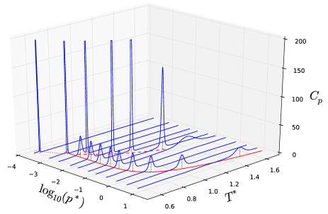
Figure 1: Demonstration of how NS can be used to calculate phase diagrams, using the case of the periodic Lennard-Jones model. NS calculations are performed at a series of pressures and phase transitions are located by peaks of the heat capacity curves (blue). The red lines show values from the literature for the melting (solid) McNeil-Watson and Wilding (2006), boiling (dashed) Kofke (1993b) and sublimation (dotted) Agrawal and Kofke (1995) curves.

In Figure 2 we compare the performance of NS to that of PT for calculating the melting and evaporation transitions. NS provides a reasonable estimate of the melting and boiling points using only $\sim 10^{8}$ energy evaluations, while parallel tempering needs many orders of magnitude more computational effort than NS to find the evaporation transition and almost two orders of magnitude more computational effort to find the melting transition. (A similar increase in computational efficiency compared with parallel tempering was found for LJ clusters Pártay et al. (2010) and hard spheres Pártay et al. (2014); Odriozola (2009).)

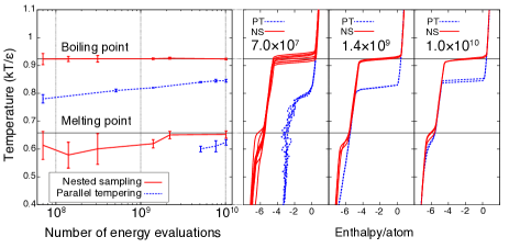
Figure 2: Performance comparison of NS and PT. Sixty-four Lennard-Jones particles were simulated at a pressure of $0.027$ (Lennard-Jones units). Both NS and PT simulations were initialised from the vapour phase. PT was performed using 128 equispaced temperature values in the range $[0.4,1.4]$. The left panel shows the estimated transition temperatures as a function of computational cost while the right panel shows the mean enthalpy as a function of temperature corresponding to three selected values of the cost.

Finally, in Figure 3 we show the phase diagram for 64 particles of Lennard Jonesium as calculated using NS with $K=640$, $L=1.6\times 10^{5}$. Comparison with the literature phase diagrams for $\sim 500$ particles confirms excellent agreement with the literature values for the evaporation transition Kofke (1993b) and also the solid-liquid and high pressure solid-vapour transitions McNeil-Watson and Wilding (2006). Below the triple point, we observe slower convergence with respect to $L$ towards literature values of the sublimation transition Agrawal and Kofke (1995). We also find the beginning of the Widom-line: the shallow line of heat capacity maxima that extends into the supercritical region. The Widom-line and our method for estimating the critical point are described in the SM SM .

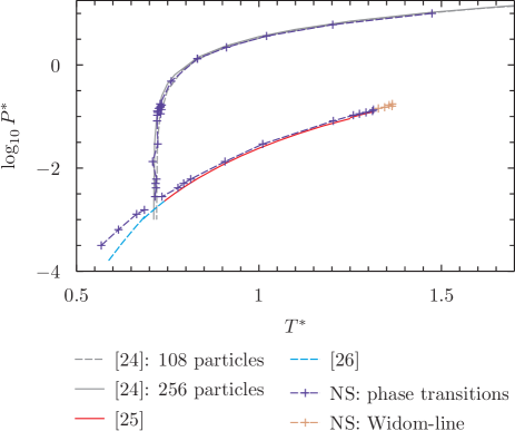
Figure 3: Phase diagram for $N=64$ Lennard-Jones particles as calculated using NS, with comparison to the literature ($N\approx 500$) phase diagram, as described in the text.

IV Results

IV.1 Aluminium

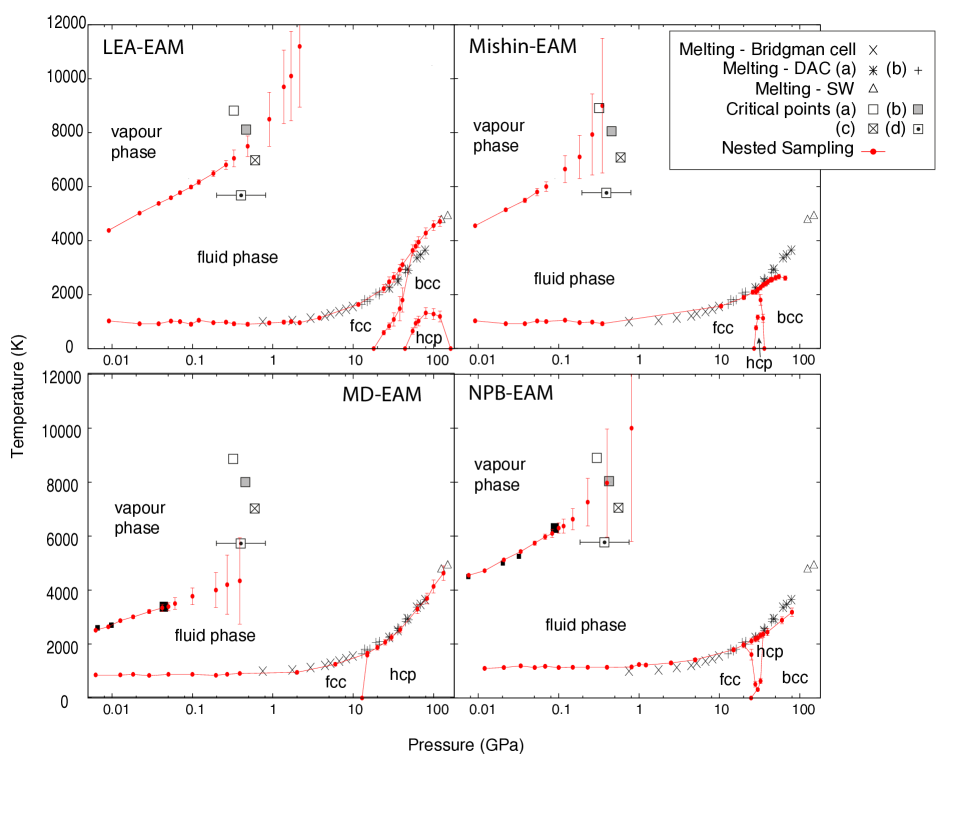
Figure 4: Phase diagrams corresponding to four EAM models of aluminium. Red symbols show the NS results, the error bars are calculated as the width at half maximum of the peaks on the heat capacity curves. On the boiling line points are connected by a solid line up to the critical point. (The method we used to estimate the critical point is described in the SM SM .) Black symbols show experimental melting points measured with Bridgman cells Errandonea (2010), with Diamond anvil cells (DAC (a) Boehler and Ross (1997) and (b) Hänström and Lazor (2000)) and shock waves (SW) Shaner et al. (1984). Different square symbols show estimates of the critical point from experiments, (a) Likalter (2002), (b) Fortov and Iakubov (2000), (c) Young and J (1971) and (d) Renaudin et al. (2003). For NPB-EAM and MD-EAM large black squares show the critical point and smaller black squares show the evaporation temperatures, all calculated using Gibbs ensemble Monte Carlo Bhatt et al. (2006). At pressures below the critical point, NS parameters $K=800$ and $L=3000$ were used (the total number of energy evaluations was $3\times 10^{9}$ for each pressure), while runs at pressures where solid-solid transitions are present required $K=3200$ and $L=15000$ (total number of energy evaluations were $4\times 10^{10}$).

In this section we apply the new algorithm to several empirical models of aluminium in order to demonstrate the capability of nested sampling to find solid-solid phase transitions without any prior knowledge of the crystal structures or even the existence of multiple stable phases. Furthermore, although the particular off-the-shelf models we use here do not reproduce the experimentally determined phase diagram of the material everywhere, the fact that nested sampling allows a direct calculation of the entire phase diagram means that in the future one could automate the optimisation of potentials to match the experimental phase diagram.

As one of the most commonly used metals, the thermodynamic properties of aluminium have been extensively studied. The melting line of aluminium has been measured up to 125 GPa Errandonea (2010); Boehler and Ross (1997); Hänström and Lazor (2000); Shaner et al. (1984), with good agreement between the different experimental techniques. Theoretical calculations have also been performed using embedded-atom type potentials Foiles et al. (1986); Voter and Chen (1987); Oh and Johnson (1988); Mei and Davenport (1992); Morris et al. (1994); Ercolessi and Adams (1994); Liu et al. (2004); Mishin et al. (1999) and ab initio methods de Wijs et al. (1998); Vočadlo and Alfè (2002); Alfè et al. (2004), the latter providing melting temperatures up to 350 GPa Bouchet et al. (2009). At ambient conditions aluminium crystallises in the face-centred-cubic (fcc) structure, but a phase transition to the hexagonal-close-packed (hcp) structure at 217 GPa has been revealed by X-ray diffraction experiments Akahama et al. (2006) and the body-centred-cubic (bcc) phase has been also produced in laser-induced microexplosions Vailionis et al. (2011). The critical points of most metals are not amenable to conventional experimental study and thus estimation of their properties is usually based upon empirical relationships between the critical temperature and other measured thermodynamic properties. In the case of aluminium these result in predictions in a wide temperature and pressure range Renaudin et al. (2003); Likalter (2002); Fortov and Iakubov (2000); Young and J (1971).

We chose four widely used models all based on the embedded-atom method (EAM): (1) the model developed by Liu et al. Liu et al. (2004) (LEA-EAM), which is an improved version of the original potential of Ercolessi and Adams Ercolessi and Adams (1994), (2) the model developed by Mishin et al. Mishin et al. (1999) using both experimental and ab initio data (Mishin-EAM), (3) the EAM of Mei and Davenport Mei and Davenport (1992) (MD-EAM) and (4) the recently modified version of the MD-EAM, reparametrised by Jasper et al. to accurately reproduce the DFT energies for Al clusters and nanoparticles of various sizes (NPB-EAM) Jasper et al. (2005).

The phase diagrams for all four models based on NS simulations with 64 particles are shown in Figure 4. The resulting critical parameters vary over a wide range for the different models. Above the critical point we observe the Widom-line, indicated by those points not linked by a solid line. Heat capacity maxima corresponding to the Widom-line become broader away from the critical point, as indicated by the larger error bars. The Widom-line and our method for estimating the critical point are described in the SM SM .

The melting lines are in a good agreement with the available experimental data up to the pressure value $p\approx 25$ GPa. Above that pressure, the melting curves diverge from the experimental results, except for the MD-EAM potential, which reproduces the melting curve remarkably well.

At higher pressures small peaks appear on the heat capacity curves below the melting temperature for all models indicating solid-solid phase transitions (see appendix B). We post-processed the samples from the NS simulations. As expected, the fcc structure was found to be stable at low pressures in all four models. However, the models differ markedly in their predictions at high pressures. The only commonality between the predicted high pressure solid phase diagrams is that the maximum predicted stable pressure for the fcc structure is far too low, both in comparison with experiment and density functional theory Akahama et al. (2006); Boettger and Trickey (1996); Sin’ko and Smirnov (2002).

IV.2 NiTi

Finally, in order to demonstrate that NS is applicable to more complex problems, we show results for a material of current scientific interest, the NiTi shape memory alloy Ji et al. (2015); Buehler et al. (1963). The shape memory effect relies on the structural phase transition from the high temperature austenitic phase to the low temperature martensitic phase Bhattacharya (2003). Studying this transition is particularly challenging with traditional free energy methods because the austenitic phase does not correspond to a local minimum of the potential energy surface. Figure 5 shows the pressure-temperature-composition phase diagram corresponding to a recent EAM model Zhong et al. (2011); Mirzaeifar et al. (2014) as computed with NS. The phase transition temperatures are within 50 K of the experimental values and reproduce the trend with compositional change. We predict a decreasing transition temperature with increasing pressure. It is notable that this potential successfully reproduces the martensitic transition temperature, despite the fact that the minimum enthalpy structure for the potential is different to the structure observed both experimentally and in DFT: here the lowest enthalpy structure (which we label B19X) is orthorhombic (see the SM SM for a description of the low enthalpy structures we identified). Thus it appears that the austenite-martensite transition temperature is not sensitive to the detailed geometry and ordering of the lowest enthalpy structures. Such empirical potentials can therefore be useful tools for studying this transition in the future.

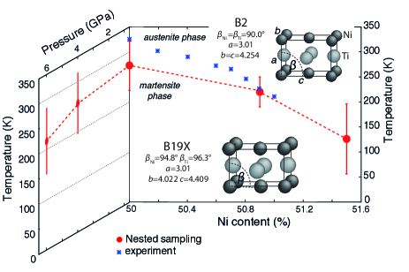
Figure 5: NiTi martensitic phase transition as a function of Ni content (at 0.66 GPa) and pressure (at 1:1 composition). The simulation cell contained 64 atoms in the cases of the 50% and 51.6% Ni compositions and 108 atoms in the case of 50.8% Ni content. NS parameters were $K=1920$, $L=10^{5}$, each data point used $10^{10}$ energy evaluations, and Ni–Ti swap moves were also included in the MC. Experimental results are taken from Frenzel et al. (2010).

V Conclusion and outlook

In summary, we have extended the nested sampling algorithm to allow simulations using fully flexible periodic boundary conditions at fixed pressure and demonstrated how it can be used to determine pressure-temperature-composition phase diagrams. In contrast to existing methods for comparing specific phases, NS explores the entire configuration space without requiring any prior knowledge about the structures of different solid phases with the only necessary input being the composition and the desired pressure and temperature ranges. This makes it the method of choice for exploring the pressure-temperature-composition space, which is the next unexplored realm naturally following much recent work in crystal structure exploration at zero temperature. Since the algorithm is run independently for different pressures and compositions, and also has excellent parallel scaling up to a number of processors equal to the number of simultaneous samples, it might even be possible to run it on ab initio models on exascale computers. Furthermore, we suggest NS is eminently suitable for validating materials models, and in the future could even play a role in the automatic optimisation of empirical models.

Appendix A Ideal gas contribution to the partition function

In this appendix we show that the ideal gas contribution to the partition function (8) asymptotically approaches zero for any positive minimum cell depth $d_{0}$, in the limit $k_{\mathrm{B}}T/pV_{0}\rightarrow 0$.

The ideal gas contribution to the partition function (8) is

$$\int_{D\left(\mathbf{h}_{0}\right)>d_{0}}\!\!\!\!\!\!\!\!\!d\mathbf{h}_{0}\delta\left(\det{\mathbf{h}_{0}}-1\right)\int_{V_{0}}^{\infty}\!\!dVV^{N}\int_{\left(0,1\right)^{3N}}\!d\mathbf{s}\,e^{-\beta pV}$$ (16)

We begin by noting that the exponential term does not depend on $E(\mathbf{s},\mathbf{h}_{0},V)$, and therefore $\int_{(0,1)^{3N}}d\mathbf{s}=1$. Thus we have

$$\int_{D\left(\mathbf{h}_{0}\right)>d_{0}}\!\!\!\!\!\!\!\!\!d\mathbf{h}_{0}\delta\left(\det{\mathbf{h}_{0}}-1\right)\int_{V_{0}}^{\infty}dVV^{N}\int_{(0,1)^{3N}}\mathrm{d}\mathbf{s}e^{-\beta pV}$$ (17)

$$=\int_{D\left(\mathbf{h}_{0}\right)>d_{0}}\!\!\!\!\!\!\!\!\!d\mathbf{h}_{0}\delta\left(\det{\mathbf{h}_{0}}-1\right)\int_{V_{0}}^{\infty}dVV^{N}e^{-\beta pV}.$$

The integral over volume $V$ evaluates to

$$\int_{V_{0}}^{\infty}dVV^{N}e^{-\beta pV}=\frac{1}{(\beta p)^{N+1}}\Gamma(N+1,\beta pV_{0})$$ (18)

where $\Gamma(N+1,\beta pV_{0})$ is the upper incomplete gamma function.

Finally we define the function $A\left(d_{0}\right)$ to be equal to the integral over $\mathbf{h}_{0}$

$$A\left(d_{0}\right)=\int_{D\left(\mathbf{h}_{0}\right)>d_{0}}\!\!\!\!\!\!\!\!\!d\mathbf{h}_{0}\delta\left(\det{\mathbf{h}_{0}}-1\right).$$ (19)

The function $A\left(d_{0}\right)$ is finite for any positive value of $d_{0}$, $A\left(1\right)=0$ and $A\left(d_{0}\right)$ diverges in the limit $d_{0}\rightarrow 0$. In the orthorhombic case, where all angles of the simulation cell are equal to $\frac{\pi}{2}$, $A\left(d_{0}\right)=\frac{9}{2}\left(\log d_{0}\right)^{2}$, with $A=1$ at $d_{0}\approx 0.62$. However at any positive value of $d_{0}$ the contribution to the partition function (8) due to volumes greater than $V_{0}$ goes to zero in the limit $k_{\mathrm{B}}T/pV_{0}\rightarrow 0$ because $\Gamma(N+1,\beta pV_{0})\rightarrow 0$ in the same limit.

Appendix B Identifying solid-solid phase transitions

The locations of phase transitions are determined solely by looking at the peaks in the heat capacity. Next, we inspect the system at temperatures either side of the phase transition. Specific phases can be identified in the following way. If no appropriate order parameter is to hand, then one picks a number of random configurations from the output of nested sampling, chosen according to their thermal weights $\Delta\chi_{i}e^{-\beta H_{i}}$, and inspects them by eye. If an appropriate order parameter is known, one can compute the free energy landscape for that order parameter. Here one proceeds by binning the weights $\Delta\chi_{i}e^{-\beta H_{i}}$ of all configurations, according to the order parameter, to create a partial sum $\Delta_{j}=\sum{\Delta\chi_{i}e^{-\beta H_{i}}}$ for each bin $j$. The free energy for each bin can then be computed as $F_{j}=-\frac{1}{\beta}\left[\log(\Delta_{j})+\log\left(\frac{\beta p}{N!}\right)+\frac{3N}{2}\log\left(\frac{2\pi m}{\beta h^{2}}\right)\right]$. In fact, simply calculating the expected enthalpy at the phase transition, and then examining the order parameter values for output configurations around that enthalpy is often sufficient to identify the crystal structures.

An example of the latter approach is shown in Figure 6 for the Mishin-EAM potential, which compares the enthalpies and $Q_{6}$ bond order parameter values for nested sampling output configurations at three different pressures. At $p=25.0$ GPa no phase transition occurs, and only fcc configurations are present. At $p=34.9$ GPa a first order phase transition occurs at the average enthalpy marked by the vertical dashed line. At that enthalpy there is a clear transition between two basins, from a first basin that corresponds to the bcc structure, to a second that corresponds to the hcp structure. Finally, at $p=37.5$ GPa no phase transition occurs and so there is no peak in the heat capacity. At this pressure the bcc structure is stable at all temperatures below the melting point. Nevertheless, the hcp structure is clearly visible as a metastable structure.

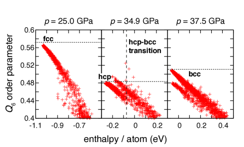
Figure 6: Identification of solid phases from inspection of an order parameter: Mishin-EAM potential for aluminium. These plots compare the enthalpies and $Q_{6}$ bond order parameter values for nested sampling output configurations at three different pressures. Nested sampling proceeds towards lower enthalpies, thus from right to left in each plot. Horizontal dotted lines show the bond order parameters for the perfect fcc, bcc and hcp phases, and the vertical dashed line shows the expected enthalpy at the solid-solid phase transition, which was located by inspecting the heat capacity and observing a peak. These results are discussed in the text.

Determining pressure-temperature phase diagrams of materials: Supplemental Material

I Detailed Monte Carlo Scheme

To understand the Monte Carlo scheme for NS in the fixed pressure ensemble with a fully flexible cell, it is helpful to first consider the Monte Carlo scheme for the fixed volume ensemble, with a fixed cell. In that case the partition function is given by

$$Z(N,V,\beta)=\frac{1}{N!}\left(\frac{2\pi m}{\beta h^{2}}\right)^{3N/2}V^{N}\int d\mathbf{s}\,e^{-\beta E\left(\mathbf{s},V\right)}.$$ (S1)

As described in previous papers Pártay et al. (2010); Burkoff et al. (2012); Martiniani et al. (2014), each iteration begins with $K$ samples distributed uniformly in $\mathbf{s}$, with $E<E_{\mathrm{limit}}$. That is to say, those $K$ samples are drawn from the distribution

$$\mathrm{Prob}\left(\mathbf{s}|E_{\mathrm{limit}}\right)=\begin{cases}\frac{1}{\chi\left(E_{\mathrm{limit}}\right)},&E\left(\mathbf{s},V\right)<E_{\mathrm{limit}}\\ 0,&\text{Elsewhere}.\end{cases}$$ (S2)

For the fixed pressure ensemble, we must explore volume and cell matrices $\mathbf{h}_{0}$, as well as the fractional coordinates $\mathbf{s}$. In particular, we calculate the integral (9) with NS.

$$\Delta_{\mathrm{NS}}(N,p,\beta,V_{0},d_{0})=\int_{D\left(\mathbf{h}_{0}\right)>d_{0}}\!\!\!\!\!\!\!\!\!d\mathbf{h}_{0}\delta\left(\det{\mathbf{h}_{0}}-1\right)\times\int_{0}^{V_{0}}\!\!dVV^{N}\int_{\left(0,1\right)^{3N}}\!d\mathbf{s}\,e^{-\beta\left[E\left(\mathbf{s},\mathbf{h}_{0},V\right)+pV\right]}$$ ( 9, revisited)

In (9) the volume has a weight $V^{N}$ with $V<V_{0}$, and $\mathbf{h}_{0}$ is constrained to a surface of determinant $1$, with $D\left(\mathbf{h}_{0}\right)>d_{0}$. Therefore we seek to generate new samples according to the distribution

$$\mathrm{Prob}\left(\mathbf{s},\mathbf{h}_{0},V|H_{\mathrm{limit}}\right)$$ (S3)

$$=\begin{cases}\frac{V^{N}\delta\left(\det{\mathbf{h}_{0}}-1\right)}{\chi\left(H_{\mathrm{limit}}\right)},&H\left(\mathbf{s},\mathbf{h}_{0},V\right)<H_{\mathrm{limit}},\>V<V_{0},\\ &D\left(\mathbf{h}_{0}\right)>d_{0}\\ 0,&\text{Elsewhere}.\end{cases}$$

As described in the paper, this can be achieved by Markov chain Monte Carlo (MCMC) sampling. MCMC walks were random sequences of the following Monte Carlo (MC) moves, which were chosen according to the probabilities (ratios) given in the paper, unless specifically stated in this Supplemental Material.

Atom moves

Single atom MC moves are performed as follows.

1. Select a single atom at random. This atom has fractional coordinates $\mathbf{s}_{i}$

2. Displace that atom’s fractional coordinates by a random vector

   $$\mathbf{s}_{i}\rightarrow\mathbf{s}_{i}+L_{s}\mathbf{\Delta_{s}}$$ (S4)

   Here $\mathbf{\Delta_{s}}$ is a 3-tuple with elements drawn independently from a uniform distribution on the interval $[-1,1]$, and $L_{s}$ is a constant that controls the step size. The size of $L_{s}$ was updated periodically during the NS calculation, as described in the next subsection, “Updating MC step lengths”.

3. Calculate the enthalpy $H_{\mathrm{trial}}=E\left(\mathbf{s},\mathbf{h}_{0},V\right)+pV$ for the system after this atom displacement.

4. Accept the displacement if $H_{\mathrm{trial}}<H_{\mathrm{limit}}$. Otherwise, the old configuration is kept.

Volume moves

Volume MC steps are as follows.

1. Propose a volume move from $V$ to $V^{\prime}$ where

   $$V^{\prime}=V+L_{V}\Delta_{V}$$ (S5)

   Here $\Delta_{V}$ is a random number drawn from the uniform distribution on the interval $[-1,1]$, and $L_{V}$ is a constant that controls the step size. The size of $L_{V}$ was updated periodically during the NS calculation, as described in the next subsection, “Updating MC step lengths”.

2. The displacement is accepted with probability $\min\left(1,\left[\frac{V^{\prime}}{V}\right]^{N}\right)$. If the displacement is accepted, continue to step 3. Otherwise, the old configuration is kept and the move ends.

3. If the displacement was accepted in step 2, calculate the enthalpy $H_{\mathrm{trial}}=E\left(\mathbf{s},\mathbf{h}_{0},V^{\prime}\right)+pV^{\prime}$ for the system after this volume displacement.

4. If $H_{\mathrm{trial}}<H_{\mathrm{limit}}$ the displacement is accepted. Otherwise, the old configuration is kept.

Lattice shear moves

The unit simulation cell $\mathbf{h}_{0}$ is sheared, subject to constraints on both the cell depth and the enthalpy. The algorithm is given in Algorithm LABEL:alg:h0_shear_mc. The size of shear steps is controlled by the parameter step_l_sh. This parameter was updated periodically during the NS calculation, as described in the next subsection, “Updating MC step lengths”.

Lattice stretch moves

The unit simulation cell $\mathbf{h}_{0}$ is stretched at fixed unit volume, subject to constraints on both the cell depth and the enthalpy. The algorithm is given in Algorithm LABEL:alg:h0_stretch_mc. The size of stretch steps is controlled by the parameter step_l_st. This parameter was updated periodically during the NS calculation, as described in the next subsection, “Updating MC step lengths”.

(Binary) atom swaps

For the NiTi alloy, we included binary (Ni–Ti) atom swaps as an additional MC proposal. The algorithm for this MC proposal is as follows:

1. Choose a random Ni atom, and a random Ti atom.

2. Swap the fractional coordinates of those two atoms.

3. Calculate the enthalpy $H_{\mathrm{trial}}=E\left(\mathbf{s},\mathbf{h}_{0},V\right)+pV$ for the system after the swap.

4. Accept the swap if $H_{\mathrm{trial}}<H_{\mathrm{limit}}$. Otherwise, the old configuration is kept.

⬇

subroutine lattice_shear_mc

! lattice shear MC step

! The input unit cell matrix is h0_in(3,3)

h0_trial = h0_in ! copy h0_in into working array

do repeat = 1, 3 ! repeat three times

h0_save = h0_trial ! save $\mathbf{h}_0$ in case of rejection

chng_vec = ranf()*3 + 1 ! randomly selected lattice

! vector. integer: 1, 2, or 3

basis = orthonormal_basis(h0_in,chng_vec)

! basis(3,2) is a pair of orthonormal vectors in the plane

! defined by the two edge vectors in h0_in other than chng_vec

pair: do

x = 2.0*(ranf() - 0.5) ! generate (x,y) pair from

y = 2.0*(ranf() - 0.5) ! inside unit circle

if (x**2 + y**2 < 1.0) exit pair

end do pair

x = x*step_l_sh ! x,y updated to uniform pair in

y = y*step_l_sh ! a circle of radius step_l_sh

h0_trial(:,chng_vec) = h0_trial(:,chng_vec)

+ x*basis(:,1) + y*basis(:,2)

! change to cell vector chng_vec is circularly symmetric

! and in the plane defined by the other two edge vectors

if ( ch(h0_trial) < mch ) h0_trial = h0_save

! trial rejected due to minimum cell depth criterion.

! cell depth of proposed cell is smaller than minimum

! allowed value: $ \ch\left(\mathbf{h}_0\right) < \mch $

end do

H_trial = H(h0_trial) ! H = configurational enthalpy

if (H_trial <= H_lim) then

h0_out = h0_trial ! accept trial

else

h0_out = h0_in ! trial rejected

! $\mathbf{h}_0$ unchanged: a null step

end if

end subroutine

⬇

subroutine lattice_stretch_mc

! lattice stretch MC step

! The input unit cell matrix is h0_in(3,3)

h0_trial = h0_in ! copy h0_in into working array

do repeat = 1, 3 ! repeat three times

h0_save = h0_trial ! save $\mathbf{h}_0$ in case of rejection

vec1 = ranf()*3 + 1 ! (vec1,vec2) is a random

vec2 = ranf()*2 + 1 ! pair of different lattice

if (vec1 == vec2) then ! vectors

vec2 = 3

end if

! u is a uniform random variable from

! [-step_l_st,step_l_st]

u = 2.0*(ranf() - 0.5)*step_l_st

! multiply edge vectors vec1, vec2 by exp(u), exp(-u)

h0_trial = h0_in

h0_trial(:,vec1) = h0_trial(:,vec1)*exp(u)

h0_trial(:,vec2) = h0_trial(:,vec1)*exp(-u)

if ( ch(h0_trial) < mch ) h0_trial = h0_save

! trial rejected due to minimum cell depth criterion.

! cell depth of proposed cell is smaller than minimum

! allowed value: $ \ch\left(\mathbf{h}_0\right) < \mch $

end do

H_trial = H(h0_trial) ! H = configurational enthalpy

if (H_trial <= H_lim) then

h0_out = h0_trial ! accept trial

else

h0_out = h0_in ! trial rejected

! $\mathbf{h}_0$ unchanged: a null step

end if

end subroutine

I.1 Updating MC step lengths

The values of the step size parameters, $L_{s}$, $L_{V}$, step_l_sh and step_l_st, were updated every $\frac{K}{2}$ iterations (recall that $K$ is the number of samples employed in the NS calculation). This corresponds to an expected reduction in the enclosed configuration space volume $\chi$ to a factor of $e^{-\frac{1}{2}}$. Each step size parameter was updated by performing a short MCMC exploration using only the corresponding type of MC proposal. The step size parameters were updated to maintain an acceptance rate in the interval $\left(0.2,0.3\right)$, and as close to $0.25$ as possible, for each MC proposal type.

Since the calculation was performed in parallel, when collecting data about the acceptance rate for each MC proposal type, each processor ran MCMC trajectories with separate, random configurations from the current sample set. In general, this avoids setting step lengths appropriate to unrepresentative regions of the bounded uniform distribution.

II Parallelisation scheme

In order to be able to benefit from supercomputing facilities efficiently, the NS algorithm has to be parallelised. Fortunately, possible parallelisation schemes come quite naturally from the method, and here we describe a scheme for parallelising within each iteration Baldock (2014). While in the serial algorithm, the new clone is decorrelated using a trajectory of walk length $L$ in each iteration, in our scheme parallelised over $N_{\mathrm{proc}}$ processors, the new clone is decorrelated using a trajectory of walk length $L/N_{\mathrm{proc}}$, along with $(N_{\mathrm{proc}}-1)$ randomly chosen configurations which are also (independently) propagated through $L/N_{\mathrm{proc}}$ steps. Thus, rather than propagating a single configuration for $L$ steps, we propagate $N_{\mathrm{proc}}$ configurations for $L/N_{\mathrm{proc}}$ steps.

III Finite size effect

In order to estimate the effect of using only 64 particles in our simulations we performed tests with 32 and 128 particles as well for both the periodic Lennard-Jones and the LEA-EAM aluminium potential models. The heat capacities of these are compared in Figure S1. The Lennard-Jones test was performed at $p=0.027\epsilon/\sigma^{3}$, below the critical point, hence both the evaporation and melting peaks are present. The aluminium test was performed at $p=11.6$ GPa, above the critical point, thus only the melting peak is present. The figure shows that increasing the number of atoms, the heat capacity peaks become narrower as expected, and the melting and evaporation transitions shift to lower and higher temperatures respectively. Of course, it would be possible to perform a finite size scaling analysis from the results of multiple Nested Sampling calculations, performed at different system sizes. However, we felt that the phase diagrams of the various aluminium models differed from each other to the extent that it was sufficient to give a rough indication of error based on the full-width-at-half-maximum of the peaks.

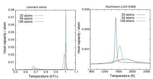
Figure S1: Magnitude of the finite size effect in case of the Lennard-Jones potential (left panel) run with parameters $K=672$ and $L=15120$, and LEA-EAM aluminium potential (right panel) with run parameters $K=1608$ and $L=10080$, as demonstrated by the heat capacity curves of systems of 32, 64 and 128 particles.

IV Lennard-Jones potentials

The benchmark comparison to parallel tempering was performed using the truncated and shifted Lennard-Jones potential Frenkel and Smit (2001). Other Lennard-Jones calculations were performed using the truncated but not shifted potential with the usual mean-field correction Frenkel and Smit (2001) beyond the cut-off radius. All Lennard-Jones calculations employed a cut-off radius $r_{c}=3\sigma$.

V Aluminium

V.1 Simulation details

The simulation cell contained 64 aluminium atoms. The same ratio of the different types of MC moves was used at every pressure. Sampling is robust with respect to the ratio of MC moves of each type, and for these aluminium calculations the ratio of MC moves (atom:volume:shear:stretch) was (16:1:1:1), rather than (N:10:1:1). The minimum allowed cell depth, $d_{0}$, was set to 0.65. Spline parameters for the LEA-EAM and Mishin-EAM potentials are only provided for configurations where no two atoms are closer than a certain, small radius. For separations smaller than this radius we made linear extrapolations to the splines. The ultra-close atomic proximity region is only relevant to the ultra-high temperature gas phase, and does not contribute to the thermodynamics of aluminium in the temperature and pressure ranges considered in this paper. Therefore the precise form of this extrapolation does not affect any of the results we show.

V.2 Heat capacity curves

Heat capacity curves calculated with Nested Sampling are shown in Figures S2, S3, S4 and S5.

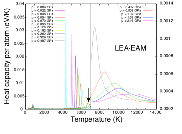
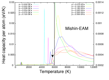
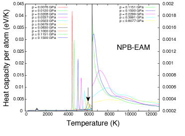
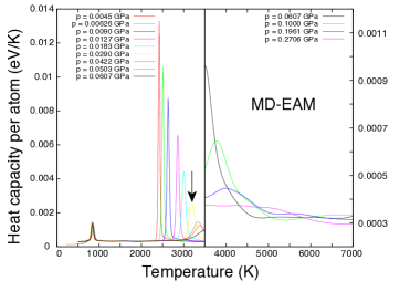
Figure S2: Aluminium heat capacity curves at lower pressures up to the end of the Widom-line for the different studied potential models. The arrows indicate the peak of the $c_{p}$ curves closest to the critical point, and in order to show the broadened peaks above that, the curves in the supercritical region are shown on a different scale (shown on the right hand side). The size of the live set and the total number of MC steps during one iteration was $K=804$ and $L=3120$, respectively.

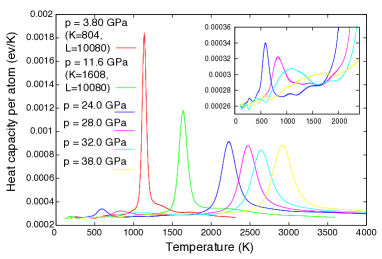
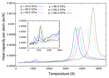
Figure S3: Aluminium heat capacity curves above the critical point for the LEA-EAM potential. The insets show the solid-solid phase transition peaks in a larger scale. The size of the live set was $K=3216$ and the total number of MC steps during one iteration was $L=15120$, or if otherwise, it is indicated in the legend.

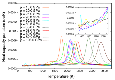
Figure S4: Aluminium heat capacity curves above the critical point for the NPB-EAM potential. The inset shows the solid-solid phase transition peaks in a larger scale. The size of the live set was $K=3216$ and the total number of MC steps during one iteration was $L=15120$.

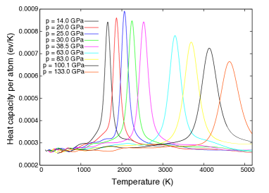
Figure S5: Aluminium heat capacity curves above the critical point for the MD-EAM potential. The size of the live set was $K=3216$ and the total number of MC steps during one iteration was $L=15120$.

V.3 Critical point and the Widom-line

To locate the critical point, we draw on the results of Bruce and Wilding Bruce and Wilding (1992). Specifically we begin from their analysis of the probability distribution for density for finite systems, in the pressure-temperature region that would contain the critical point in an infinite system. For a finite system at and below the critical point the density distribution for temperatures corresponding to maxima of the heat capacity appears as a bimodal distribution. Above the critical point (along the Widom-line), the distribution transitions quickly to a unimodal distribution. In the context of a phase diagram, our location of the critical point appears quite precise, but in fact our sampling of the pressure axis is relatively sparse compared to the width of the scaling region around the critical point, since we are inspecting the system across pressures spanning many orders of magnitude. Therefore, between adjacent pressure values the density distribution transitions rapidly between being bimodal and unimodal. We chose the lowest pressure for which the distribution is clearly unimodal as an upper bound for the critical pressure. The corresponding upper bound for the critical temperature was taken to be the temperature at which the heat capacity, Cp, is its local maximum at that pressure.

According to textbook definitions, beyond the critical point a single fluid phase is defined. However, response functions such as the heat capacity, thermal expansion coefficient and compressibility continue to exhibit maxima into the supercritical region. Lines of these maxima, which spread out from the critical point are called the Widom-lines. If one moves away from the critical point, the different Widom-lines rapidly diverge from one another, and the maxima themselves become quickly smeared and disappear, in case of the heat capacity at $T\approx 2.5T_{c}$ and $p\approx 10p_{c}$ Brazhkin et al. (2011). The same tendency can be observed in our Nested Sampling results, see Fig. S2.

By calculating the expected density as a function of temperature, the equation-of-state can be calculated using Nested Sampling. These are plotted for the low pressure region together with Gibbs ensemble Monte Carlo simulation results from Ref Bhatt et al. (2006) in Figure S6. The critical parameters for the different aluminium potentials determined by Nested Sampling are summarised in Table S1.

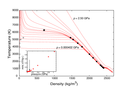
Figure S6: Density-temperature phase diagram of aluminium with the NPB-EAM potential. Red lines show the Nested Sampling results at different pressures: 0.000402 GPa, 0.0012 GPa, 0.0208 GPa, 0.0337 GPa, 0.0503 GPa, 0.0679 GPa, 0.0830 GPa, 0.100 GPa, 0.115 GPa, 0.150 GPa, 0.230 GPa, 0.399 GPa, 0.807 GPa, 1.0 GPa, 2.5 GPa. The curve corresponding to the critical pressure is shown by a dashed line. Black and open circles show the liquid and vapour densities respectively, from Bhatt et al. (2006), with a black star showing their estimate of the critical point. The inset shows the minimum value of the derivative of the curves obtained by Nested Sampling, with the arrow indicating the pressure value where the plateau between vapour and liquid phases diminish at the critical point.

Table S1: Critical temperature and pressure as estimated from the Nested Sampling calculations for the different potential models. Numbers in parenthesis show GEMC results from Ref. Bhatt et al. (2006) for comparison.

	$T_{c}$ (K)	$p_{c}$ (GPa)
LEA-EAM	$6810\pm 170$	0.262
Mishin-EAM	$5800\pm 140$	0.054
NPB-EAM	$6100\pm 150$ ($6299\pm 48$)	0.083 ($0.0896\pm 0.0019$)
MD-EAM	$3340\pm 140$ ($3381\pm 13$)	0.042 ($0.044\pm 0.002$)

VI NiTi

Here we discuss the lowest enthalpy structures we identified for the EAM potential used to describe NiTi Zhong et al. (2011). The enthalpic and energetic ordering of these structures is the same for all pressures considered in this paper. Therefore we shall restrict our discussion to their energy values.

The EAM potential gives rise to a number of low energy structures that show some similarity to the experimentally observed low temperature structure (B19’) and to other structures found using DFT (namely B19 and BCO). The lowest energy structure of the EAM potential is orthorhombic, but with significant displacement of the atoms from their high temperature average B2 positions. Table S2 below gives the structural parameters of the three structures with the lowest energies. In addition, we found that a multitude of local minima exist between just 10 and 15 meV/atom above the lowest energy structure. The symmetries of these configurations were identified using the findsym package Stokes and Hatch (2005).

Table S2: Low energy structures of NiTi according to the EAM potential. Lattice vectors are in Å, energies are per atom and are relative to the B2 phase.

Symmetry	$a$	$b$	$c$	$\beta$	Wyckoff positions	Energy (meV)
Pm$\bar{3}$m (B2)	3.0098	3.0098	3.00980	90	Ni: a, Ti: b	0
Pmm2 (B19X)	4.02186	4.40909	3.01484	90	Ni: b (z=-0.04073), c (z=0.04305) Ti: a (z=-0.4434), d (z=0.4458)	-53.8
C2/m (B19)	4.46697	4.02169	3.00532	98.1	Ni: a, Ti: d	-51.1
P21/m (BCO)	2.99360	4.00083	4.88392	107.8	Ni: e (x=0.08755, z=-0.3249) Ti: e (x=0.3583, z=0.2167)	-46.8

References

- Panagiotopoulos (1987) A. Z. Panagiotopoulos, Mol. Phys. 61, 813 (1987).
- Kofke (1993a) D. A. Kofke, Mol. Phys 78, 1331 (1993a).
- Skilling (2004) J. Skilling, AIP Conf. Proc. 735, 395 (2004).
- Skilling (2006) J. Skilling, Bayesian Anal. 1, 833 (2006).
- Swendsen and Wang (1986) R. H. Swendsen and J. S. Wang, Phys. Rev. Lett. 57, 2607 (1986).
- Frantz et al. (1990) D. D. Frantz, D. L. Freemann, and J. D. Doll, J. Chem. Phys. 93, 2769 (1990).
- Wang and Landau (2001) F. Wang and D. P. Landau, Phys. Rev. Lett. 86, 2050 (2001).
- Allen and Tildesley (2012) M. Allen and D. Tildesley, Computer Simulation in Chemical Physics, Nato Science Series C: (Springer Netherlands, 2012).
- Feroz and Hobson (2008) F. Feroz and M. P. Hobson, Mon. Not. R. Astron. Soc. 384, 449 (2008).
- Pártay et al. (2010) L. B. Pártay, A. P. Bartók, and G. Csányi, J. Phys. Chem. B 114, 10502 (2010).
- Pártay et al. (2014) L. B. Pártay, A. P. Bartók, and G. Csányi, Phys. Rev. E 89, 022302 (2014).
- Burkoff et al. (2012) N. S. Burkoff, C. Várnai, S. A. Wells, and D. L. Wild, Biophys. J. 102, 878 (2012).
- Do et al. (2011) H. Do, J. D. Hirst, and R. J. Wheatley, J. Chem. Phys. 135, 174105 (2011).
- Do et al. (2012) H. Do, J. D. Hirst, and R. J. Wheatley, J. Phys. Chem. 116, 4535 (2012).
- Do and Wheatley (2013) H. Do and R. J. Wheatley, J. Chem. Theory Comput. 9, 165 (2013).
- Wilson et al. (2015) B. A. Wilson, L. D. Gelb, and S. O. Nielsen, J. Chem. Phys. 143, 031034 (2015).
- Martiniani et al. (2014) S. Martiniani, J. D. Stevenson, D. J. Wales, and D. Frenkel, Phys. Rev. X 4, 031034 (2014).
- Brewer et al. (2010) B. J. Brewer, L. B. Pártay, and G. Csányi, Stat. Comput. 21, 649 (2010).
- Martyna et al. (1994) G. J. Martyna, D. J. Tobias, and M. L. Klein, J. Chem. Phys. 101, 4177 (1994).
- Brooks et al. (2011) S. Brooks, A. Gelman, G. Jones, and X.-L. Meng, Handbook of Markov Chain Monte Carlo (CRC press, 2011).
- Frenkel and Smit (2001) D. Frenkel and B. Smit, Understanding Molecular Simulation: From Algorithms to Applications (Elsevier Science, 2001).
- Tuckerman (2008) M. Tuckerman, Statistical Mechanics and Molecular Simulations (Oxford University Press, 2008).
- (23) See Supplemental Material at [URL will be inserted by publisher] for the detailed Monte Carlo scheme, parallelisation scheme, and additional results and details including treatment of the critical point, Widom-line, and density-temperature phase diagrams.
- McNeil-Watson and Wilding (2006) G. C. McNeil-Watson and N. B. Wilding, J. Chem. Phys. 124, 064504 (2006).
- Kofke (1993b) D. A. Kofke, J. Chem. Phys. 98, 4149 (1993b).
- Agrawal and Kofke (1995) R. Agrawal and D. A. Kofke, Mol. Phys. 85, 43 (1995).
- Odriozola (2009) G. Odriozola, J. Chem. Phys. 131, 144107 (2009).
- Errandonea (2010) D. Errandonea, J. App. Phys. 108, 033517 (2010).
- Boehler and Ross (1997) R. Boehler and M. Ross, Earth Planet. Sci. Lett. 153, 1 (1997).
- Hänström and Lazor (2000) A. Hänström and P. Lazor, J. Alloys Compd. 305, 209 (2000).
- Shaner et al. (1984) J. W. Shaner, J. M. Brown, and R. G. McQueen, “Melting of metals above 100 gpa,” in High Pressure in Science and Technology, edited by C. Homan, R. K. MacCrone, and E. Whalley (Amsterdam: North-Holland, 1984) pp. 137–141.
- Likalter (2002) A. A. Likalter, Physica A 311, 137 (2002).
- Fortov and Iakubov (2000) V. Fortov and I. Iakubov, The Physics of Non-ideal Plasma (World Scientific, 2000).
- Young and J (1971) D. A. Young and A. B. J, Phys. Rev. A 3, 364 (1971).
- Renaudin et al. (2003) P. Renaudin, C. Blancard, J. Clérouin, G. Faussurier, P. Noiret, and V. Recoules, Phys. Rev. Lett. 91, 075002 (2003).
- Bhatt et al. (2006) D. Bhatt, A. W. Jasper, N. E. Schultz, J. I. Siepmann, and D. G. Truhlar, J. Am. Chem. Soc. 128, 4224 (2006).
- Foiles et al. (1986) S. M. Foiles, M. I. Baskes, and M. S. Daw, Phys. Rev. B 33, 7983 (1986).
- Voter and Chen (1987) A. F. Voter and S. P. Chen, Mater. Res. Soc. Symp. Proc. 82, 175 (1987).
- Oh and Johnson (1988) D. J. Oh and R. A. Johnson, J. Mater. Res. 3, 471 (1988).
- Mei and Davenport (1992) J. Mei and J. W. Davenport, Phys. Rev. B 46, 21 (1992).
- Morris et al. (1994) J. R. Morris, C. Z. Wang, K. M. Ho, and C. T. Chan, Phys. Rev. B 49, 3109 (1994).
- Ercolessi and Adams (1994) F. Ercolessi and J. B. Adams, Europhys. Lett. 26, 583 (1994).
- Liu et al. (2004) X.-Y. Liu, F. Ercolessi, and J. B. Adams, Model. Simul. Mater. Sci. Eng. 12, 665 (2004).
- Mishin et al. (1999) Y. Mishin, D. Farkas, M. J. Mehl, and D. A. Papaconstantopoulos, Phys. Rev. B 59, 3393 (1999).
- de Wijs et al. (1998) G. A. de Wijs, G. Kresse, and M. J. Gillan, Phys. Rev. B 57, 8223 (1998).
- Vočadlo and Alfè (2002) L. Vočadlo and D. Alfè, Phys. Rev. B 65, 214105 (2002).
- Alfè et al. (2004) D. Alfè, L. Vočadlo, G. D. Price, and M. J. Gillan, J. Phys. Condens. Matter 16, S973 (2004).
- Bouchet et al. (2009) J. Bouchet, F. Bottin, G. Jomard, and G. Zérah, Phys. Rev. B 80, 094102 (2009).
- Akahama et al. (2006) Y. Akahama, M. Nishimura, K. Kinoshita, H. Kawamura, and Y. Ohishi, Phys. Rev. Lett. 96, 045505 (2006).
- Vailionis et al. (2011) A. Vailionis, E. G. Gamaly, V. Mizeikis, W. Yang, A. V. Rode, and S. Juodkazis, Nature Commun. 2, 445 (2011).
- Jasper et al. (2005) A. W. Jasper, N. E. Schultz, and D. G. Truhlar, J. Phys. Chem. B 109, 3915 (2005).
- Boettger and Trickey (1996) J. C. Boettger and S. B. Trickey, Phys. Rev. B 53, 3007 (1996).
- Sin’ko and Smirnov (2002) G. Sin’ko and N. Smirnov, J. Phys. Condens. Matter 14, 6989 (2002).
- Ji et al. (2015) Y. Ji, D. Wang, X. Ding, K. Otsuka, and X. Ren, Phys. Rev. Lett. 114, 055701 (2015).
- Buehler et al. (1963) W. J. Buehler, J. W. Gilfrich, and R. C. Wiley, J. Appl. Phys. 34, 1475 (1963).
- Bhattacharya (2003) K. Bhattacharya, Microstructure of martensite: why it forms and how it gives rise to the shape-memory effect (Oxford University Press, 2003).
- Zhong et al. (2011) Y. Zhong, K. Gall, and T. Zhu, J. App. Phys. 110, 033532 (2011).
- Mirzaeifar et al. (2014) R. Mirzaeifar, K. Gall, T. Zhu, A. Yavari, and R. DesRoches, J. Appl. Phys. 115, 194307 (2014).
- Frenzel et al. (2010) J. Frenzel, E. George, A. Dlouhy, C. Somsen, M.-X. Wagner, and G. Eggeler, Acta Mater. 58, 3444 (2010).

References

- Pártay et al. (2010) L. B. Pártay, A. P. Bartók, and G. Csányi, J. Phys. Chem. B 114, 10502 (2010).
- Burkoff et al. (2012) N. S. Burkoff, C. Várnai, S. A. Wells, and D. L. Wild, Biophys. J. 102, 878 (2012).
- Martiniani et al. (2014) S. Martiniani, J. D. Stevenson, D. J. Wales, and D. Frenkel, Phys. Rev. X 4, 031034 (2014).
- Baldock (2014) R. J. N. Baldock, Classical Statistical Mechanics with Nested Sampling, Ph.D. thesis, University of Cambridge (2014).
- Frenkel and Smit (2001) D. Frenkel and B. Smit, Understanding Molecular Simulation: From Algorithms to Applications (Elsevier Science, 2001).
- Bruce and Wilding (1992) A. D. Bruce and N. B. Wilding, Phys. Rev. Lett. 68, 193 (1992).
- Brazhkin et al. (2011) V. V. Brazhkin, Y. D. Fomin, A. G. Lyapin, V. N. Ryzhov, and E. N. Tsiok, J. Phys. Chem. B 115, 14112 (2011).
- Bhatt et al. (2006) D. Bhatt, A. W. Jasper, N. E. Schultz, J. I. Siepmann, and D. G. Truhlar, J. Am. Chem. Soc. 128, 4224 (2006).
- Zhong et al. (2011) Y. Zhong, K. Gall, and T. Zhu, J. App. Phys. 110, 033532 (2011).
- Stokes and Hatch (2005) H. T. Stokes and D. M. Hatch, J. Appl. Crystallogr. 38, 237 (2005).