050002 2013 G. Mindlin 050002

We discuss the historic mortality record corresponding to the initial focus of the yellow fever epidemic outbreak registered in Buenos Aires during the year 1871 as compared to simulations of a stochastic population dynamics model. This model incorporates the biology of the urban vector of yellow fever, the mosquito Aedes aegypti, the stages of the disease in the human being as well as the spatial extension of the epidemic outbreak. After introducing the historical context and the restrictions it puts on initial conditions and ecological parameters, we discuss the general features of the simulation and the dependence on initial conditions and available sites for breeding the vector. We discuss the sensitivity, to the free parameters, of statistical estimators such as: final death toll, day of the year when the outbreak reached half the total mortality and the normalized daily mortality, showing some striking regularities. The model is precise and accurate enough to discuss the truthfulness of the presently accepted historic discussions of the epidemic causes, showing that there are more likely scenarios for the historic facts.

A mathematically assisted reconstruction of the initial focus of the yellow fever outbreak in Buenos Aires (1871)

99 inst1 Departamento de Computación, Facultad de Ciencias Exactas y Naturales (FCEN), Universidad de Buenos Aires (UBA) and CONICET. Intendente Güiraldes 2160, Ciudad Universitaria, C1428EGA Buenos Aires, Argentina. inst2 Departamento de Física, FCEN–UBA and IFIBA–CONICET. 1428 Buenos Aires, Argentina. inst3 Departamento de Ecología, Genética y Evolución, FCEN–UBA and IEGEBA–CONICET. 1428 Buenos Aires, Argentina.

1 Introduction

Yellow fever (YF) is a disease produced by an arthropod borne virus (arbovirus) of the family flaviviridae and genus Flavivirus. The arthropod vector can be one of several mosquitoes and the usual hosts are monkeys and/or people. Wild mosquitoes of genus Haemagogus, Sabetes and Aedes are responsible for the transmission of the virus among wild monkeys, such as the Brown Howler Monkey (Alouatta guariba) associated to recent outbreaks of YF in Brazil, Paraguay and Argentina [1]). In contrast, urban YF is transmitted by a domestic and anthropophilic mosquito, Aedes aegypti, human beings being the host [2]. Aedes aegypti is a tree hole mosquito, with origins in Africa, that has been dispersed through the world thanks to its association with people.

During the end of the XVIII and the XIX centuries, YF caused large urban outbreaks in the Americas from Boston (1798), New York (1798) and Philadelphia (1793, 1797, 1798, 1799) in the North [3] to Montevideo (1857) and Buenos Aires (1858, 1870, 1871) [4] in the South. These historical episodes arise as ideal cases for testing the capabilities of YF models in urban settings. Is it possible to reconstruct the evolution of one of these epidemic outbreaks? Can enough information be recovered to produce a thorough test on the models? This is seldom the case, for example, for the study of the Memphis (1878) epidemic, with over 10000 casualties, only 1965 were considered potentially usable [5]. In contrast, the records of the outbreak in Buenos Aires 1871, unearthed and digitized for this work, left us with an amount of 1274 death cases located in time and space for the initial focus in the quarter of San Telmo, about 78% of the total mortality in the quarter [6]. According to the 1869 national census [7] Buenos Aires had 177787 inhabitants, 12329 of them living in San Telmo, about half of them just immigrated into the country mostly from Europe.

In this work, we will compare the initial development of the epidemic outbreak (Buenos Aires, 1871) with the simulations resulting from an eco-epidemiological model developed in Refs. [8, 9, 10], testing the worth of the predictive model.

The simulations were performed under a number of assumptions, most of them essentially forced by the lack of better information. We will assume that:

1. Now and before, YF is the same illness, i.e., we can use current information on YF development such as: the average extent of the incubation, infection, recovery, and toxic periods, as well as the mortality level in 1871. In other words, the virus presents no substantial changes since 1871 to present days. We do not expect this hypothesis to be completely correct: the YF virus is an RNA-virus as opposed to the stable DNA-viruses, as such, mutations in about 140 years of continuous replications in mosquitoes and primates can hardly be ruled out. Furthermore, present-day YF has been subject to different evolutionary pressures than the YF in the XIX century. While in the XIX century yellow fever circulated continuously in human populations, today the wild part of the cycle involving wild populations of monkeys plays a substantial role.

2. The epidemic was transmitted by Aedes aegypti. There is no evidence of this fact since the scientific society and medical doctors in general were not aware of the role played by the mosquito until the confirmation given by Reed [3] of Finlay’s ideas [11].

   We assume that Aedes aegypti has not changed since then, and/or there are no substantial changes in the life cycle, vector capabilities and adaptation between the (assumed) population in 1871 and present-day populations in Buenos Aires city. After the eradication campaign (1958–1965) [14], Aedes aegypti was eradicated from Buenos Aires [15]. Hence, the present populations result from a re-infestation and they are not the direct descendants of the mosquitoes population of 1871.

3. Lacking time statistics for the duration of the different stages in the development of the illness, reproduction of the virus and life cycle of the mosquito, we use, as distribution for such events, a maximum likelihood distribution subject to the constrain of the average value for the cycle. In short, we use exponentially distributed times for the next event for all type of events.

4. Finally, and most importantly, we assume that the human population mobility is not a factor in the local spread of the disease. We anticipate one of our conclusions: this assumption is likely to be false for the full development of the epidemic outbreak but seems reasonable for the early (silent) development. The study of the secondary foci of the epidemic outbreak merits a detailed analysis of the social and political circumstances related to human mobility and it is beyond the possibilities of this study.

Since we want the test to be as demanding as possible, more information is needed to simulate the outbreak eliminating sources of ambiguity and parameters to be fitted using the same test data. We recovered the following information:

1. Estimations of daily temperatures. They are relevant since the temperature regulates the developmental rates of the mosquitoes.

2. A very rough, anecdotal, estimation of the availability of breeding sites (BS) that, ultimately, control the carrying capacity of the environment, the number of vectors and the infection rate.

3. Human populations discriminated by block in the city.

4. Estimations of the date of arrival of the virus to the city, putting bounds to the reasonable initial conditions for the simulation.

This climatological, social and historical information represents a determining part of the reconstruction as it is integrated into the model jointly with the entomological and medical information to produce stochastic simulations of possible outbreaks to be compared with the historic records of casualties.

We will show that the model predicts large probabilities for the occurrence of YF in the given historical circumstances and it is also able to answer why a minor outbreak in 1870 did not progress towards a large epidemic. The total number of deaths and the time-evolution of the death record will be shown to agree between the historical record and the simulated episodes as well, within the original focus.

The rest of the manuscript will be organized as follows: we will begin with the description of YF in section II, including the eco-epidemiological model. In section III, we will address the relevant climatological, social and historical aspects. In section IV, we will explore the sensitivity of the model to initial conditions and the number of available breeding sites, discussing the statistics more clearly influenced by vector abundance. The historic mortality records and the simulated records are compared in section 5. We will finally discuss the performance of the model in section 6

2 The disease

We will simply quote the fact sheet provided by the World Health Organization [16] as the standardized description:

“YF is a viral disease, found in tropical regions of Africa and the Americas. It principally affects humans and monkeys, and is transmitted via the bite of Aedes mosquitoes. It can produce devastating outbreaks, which can be prevented and controlled by mass vaccination campaigns.

The first symptoms of the disease usually appear 3–6 days after infection. The first, or acute, phase is characterized by fever, muscle pain, headache, shivers, loss of appetite, nausea and vomiting. After 3–4 days, most patients improve and symptoms disappear. However, in a few cases, the disease enters a toxicphase: fever reappears, and the patient develops jaundice and sometimes bleeding, with blood appearing in the vomit (the typical vomito negro). About 50% of patients who enter the toxic phase die within 10–14 days”.

We add that the remission period lasts between 2 and 48 hours [17], and as it was mentioned in the introduction, not only Aedes mosquitoes transmit the disease.

2.1 The model

The yellow fever model is rather similar to the already presented dengue model [10], the similarity corresponds to the fact that dengue is produced by a Flavivirus as well, it is transmitted by the same vector and follows the same clinical sequence in the human being, although with substantially lesser mortality.

The model describes the life cycle of the mosquito [8] and its dispersalafter a blood meal, seeking oviposition sites [9]. The mosquito goes through several stages: egg, larva, pupa, adult (non parous), flyer (i.e., the mosquito dispersing) and adult (parous). In each stage, the mosquito can die or continue the cycle with a transition rate between the subpopulations that depends on the temperature. The mortality in the larva stage is nonlinear and it regulates the population as a function of the availability of breeding sites. Thus, the transitions from adult to flyer are associated with blood meals, the event that can transmit the virus from human to mosquito and vice-versa. From the epidemiological point of view, the mosquito follows a SEI sequence (Susceptible, Exposed —extrinsic period—, Infective). Correspondingly, the adult populations are subdivided according to their status with respect to the virus. We assume that there is no vertical transmission of the virus and eggs, larvae, pupae and non parous adults are always susceptible.

The humans are subdivided in subpopulations according to their status with respect to the illness as: susceptible (S), exposed (E), infective (I), in remission (r), toxic (T) and recovered (R). The temporary remission period is followed by recovery with a probability between 0.75 and 0.85 or a toxic period (probability 0.25 to 0.15) which ends half of the times in death and half of the times in recovery. The yellow fever model differs in the structure from the dengue model in Ref. [10], as the human part of the dengue model is SEIR and the yellow fever model is SEIrRTD. However, the additional stages do not alter the evolution of the epidemic since the “in remission”, toxic and dead stages do not participate in the transmission of the virus. The YF parameters are presented in Table 1.

Period	value	range
Intrinsic Incubation (IIP)	4 days	3–6 days
Extrinsic Incubation (EIP)	10 days	9–12 days
Human Viremic (VP)	4 days	3–4 days
Remission (rP)	1 days	0–2 days
Toxic (tP)	8 days	7–10 days

Probability	value	range
Recovery after remission (rar)	0.75	0.75–0.85
Mortality for toxic patients (mt)	0.5
Transmission host to vector (ahv)	0.75
Transmission vector to host (avh)	0.75

Table 1: Parameters (mean value of state) adopted for YF. The range indicated is taken from PAHO [17].

The model is compartmental, all populations are counted as non-negative integers numbers and evolve by a stochastic process in which the time of the next event is exponentially distributed and the events compete with probabilities proportional to their rates in a process known as density-dependent-Poisson-process [18]. The model can be understood qualitatively with the scheme of the Fig. 1. The model equations are summarized in Appendix A.

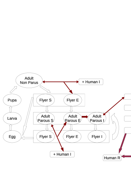
Figure 1: Scheme of the yellow fever model. On the left side, the evolution of the mosquito and, on the right side, the evolution of human subpopulations. Hollow arrows indicate the progression through the life cycle of the mosquito following the sequence: egg, larva, pupa, adult (non-parous), flyer, adult (parous) and the repetition of the two last steps. The mortality events are not shown to lighten the scheme. Eggs are laid in the transition from flyer to adult. The adult mosquito populations are subdivided according to their status with respect to the virus as: susceptible (S), exposed (E) and infective (I). The virus is transmitted from mosquitoes to humans and vice-versa in the transition from adult to flyer (blood meal) when either the mosquito or the human is infective and the other susceptible (red arrows). The red bold arrows indicate the progression of the disease, from exposed to infective in the mosquito and, in humans, following the sequence: exposed (E), infective (I), in remission (r), toxic, recovered (R) or dead.

The city is divided in blocks, roughly following the actual division (see Fig. 2). The human populations are constrained to the block while the mosquitoes can disperse from block to block.

3 Historical, social and climatological information

3.1 When and how the epidemic started

The YF outbreak in Buenos Aires (1871) was one of a series of large epidemic outbreaks associated to the end of the War of the Triple Alliance or Paraguayan war. The war confronted Argentina, Brazil and Uruguay (the three allies) on one side and Paraguay on the other side, and ended by March, 1870. By the end of 1870, Asunción, Paraguay’s capital city, was under the rule of the Triple Alliance. The return of Paraguay’s war prisoners from Brazil (where YF was almost endemic at that time) to Asunción triggered a large epidemic outbreak [4]. The allied troops received their main logistic support from Corrientes (Argentina), a city with 11218 inhabitants according to the 1869 census [7], located about 300 km south of Asunción (following the waterway) and 1000 km north of Buenos Aires along the Paraná river (see Fig. 3). On December 14, 1870, the first case of YF was diagnosed in Corrientes [19], and a focus developed around this case imported from Asunción. According to some sources, the epidemic produced panic, resulting in about half the population leaving the city between December 15 and January 15 [20]. However, other historical reasons might have played a relevant role since the city of Corrientes was under the influence and ruling of Buenos Aires, while in the farmlands, the General Ricardo López Jordan was commanding a rebel army (a sequel of Argentina civil wars and the war of the Triple Alliance). The subversion ended with the battle of Ñaembé, about 200 km east of Corrientes, on January 26, 1871.

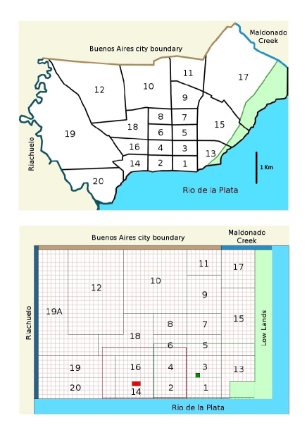
Figure 2: Police districts from a map of the time and computer representation. The red colored area in district 14 (San Telmo) are the two blocks where the 1871 epidemic started. The green colored area in district 3 is the block where the Hotel Roma was and where the 1870 focus began (see section 55.3). The red and green lines sourround the region simulated for the 1871 epidemics and the 1870 focus, respectively. Notice that districts 15 and 13 disagree in the maps. The computer representation follows the information in Ref. [21] from where the population information was obtained.

Putting things in perspective, we must realize that in those times, YF was recognized only in its toxic stage associated to the black vomit, it is then perfectly plausible that recently infected individuals would have left Corrientes and Asunción reaching Buenos Aires, despite quarantine measures that were late and leaky [22, 4]. The death toll in Corrientes was of 1289 people in the city (and about 700 more in places around the city) [20], representing a 11,5% of the population (notice that this number is not consistent with current numbers in use by WHO [17] which indicate a 7.5% of mortality in diagnosed cases of YF but is well in line with historical reports [23] of 20% to 70% mortality in diagnosed cases —the statistical basis has changed with the improved knowledge of early, not toxic, YF cases.

According to this historical view, the initial arrival of infectious people to Buenos Aires happened, more likely, during December 1870 and January 1871. In his study of the YF epidemic, written twenty three years after the epidemic outbreak, José Penna (MD) [4] quotes the issue of the journal “Revista Médico Quirúrgica”, published in Buenos Aires on December 23, 1870 [24], which presents a report regarding the sanitary situation during the last fifteen days, indicating the emergence of a “bilious fever” and a general tendency of other fevers to produce icterus or jaundice. In the next issue, dated January 8, 1871, the “Revista” indicates an important increase in the number of bilious fever cases reported [22]. In a separate article, the doctors call the attention on how easily and how often the quarantine to ships coming from Paraguay is avoided, and calls for strengthening the measures. Penna indicates that the “bilious fever” (not a standard term in medicine) likely corresponded to milder cases of YF. We will term this idea “Penna’s conjecture” and will come back to it later.

For our initial guess, we considered this information as evidence that the epidemic outbreak started during December, 1870. Exploring the model, and arbitrarily, we took December 16, 1870, as the time to introduce two infectious people with YF in the simulations, at the blocks where the mortality started. Yet, an educated guess for Penna’s conjecture is to consider the 3–6 days needed from infection to clinical manifestation and the 9–12 days of the extrinsic cycle. Hence, since the first clinical manifestations of transmitted YF happened between December 11–23, we would guess the infected people arriving somewhere between November 21 and December 11.

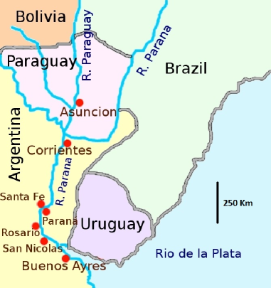
Figure 3: A 1870 map [25] showing Asunción next to the Paraguay river, Corrientes and Rosario next to the Paraná river and Buenos Aires (spelled Buenos Ayres) next to the Rio de la Plata.

Yet, we must take into account that Penna’s conjecture contrasts with the conjectures presented by MD Wilde and MD Mallo, members of the Sanity committee in charge during the YF epidemic. Wilde and Mallo advocated for the spontaneous origin of the disease, very much in line with the theories of miasmas in use in those times, theories that guided the sanitary measures taken [19]. Wilde and Mallo also argued that Asunción could not be the origin of the epidemic, because of their belief that the ten or fifteen days quarantine (counting since the last port touched) was enough to avoid the propagation of the disease. This belief contrasts with the experience of 1870 (in Buenos Aires) where a ten day quarantine was not enough to prevent a minor epidemic [4]. Nevertheless, the quarantine measures werefully implemented in Corrientes by December 31, 1870. The measures were later lifted because of the epidemic in Corrientes and implemented at ports down the Paraná river, being completed nearby Buenos Aires (ports of La Conchas, Tigre, San Fernando and “La Boca” within Buenos Aires city) by mid-February when the epidemic was in full development in Buenos Aires according to the port sanitary authorities, Wilde and Mallo [19].

Being Corrientes the source of infected people can hardly be disregarded. With about 5000 people leaving the city between December 15 and January 15 [19], a city where YF was developing.

According to Wilde and Mallo [19], there were (non-fatal?) YF cases in Buenos Aires as early as January 6, 1871, reported by MDs Argerich and Gallarani as well as documented cases of YF death after disembarking in Rosario (200 km North of Buenos Aires along the Paraná river) having boarded in Corrientes.

3.2 Breeding sites

One of the key elements in the reconstruction and simulation of an epidemic transmitted by mosquitoes is to have an estimation of their numbers which will be reflected directly in the propagation of the epidemic. In the mosquito model [8], this number is regulated by the quality and abundance of breeding sites. The production of a single breeding site, normalized to be a flower pot in a local cemetery, was taken as unit in Ref. [8] and the number of breeding sites measured in this unit roughly corresponds to half a liter of water.

The Aedes aegypti population in monitored areas of Buenos Aires, today, is compatible with about 20 to 30 breeding sites per block [9]. Estimating the number of sites available for breeding today is already a difficult task, the estimation of breeding sites available in 1871 is a nearly impossible one. In what remains of this subsection, we will try to get a very rough a-priori estimate.

District	Population/$(100\text{ m})^{2}$	$\text{BS}/(100\text{ m})^{2}$
1	339	391.0
2	279	300.0
3	428	522.0
4	353	443.0
5	330	430.0
6	259	365.0
13	160	196.0
14	224	300.0
15	90	157.0
16	165	316.0
18	23	52.0
19	13	26.0
20	30	52.0

Table 2: Population data. Buenos Aires, 1869 [7]. Population density by police district (see Fig. 2) and equivalent breeding sites, BS, originally estimated as proportional to the house density in the police district.

A very important difference between those days and the present corresponds to the supply of fresh water which today is taken from the river, processed and distributed through pipes; but in those days, it was an expensive commodity taken from the river by the “waterman” and sold to the customers who, in turn, had to let it rest so that the clay in suspension decanted to the bottom of the vessel (a process that takes at least 3 days). Additionally, there were some wells available but the water was (is) of low quality (salty). The last, and rather common resource [19, 26], was the collection of rain water in cisterns.

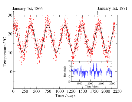
Figure 4: Average daily temperature and periodic approximation fitted accordng to Eq. (1), $t=0$ corresponds to January 1, 1866. The inset shows the difference between the measured temperatures and the fit (residuals) during 1871.

3.3 Temperature reconstruction

Aedes aegypti developmental times depend on temperature. Although it would seem reasonable to use as substitute of the real data of the average temperature registered since systematic data collection began, records of temperature in those times were kept privately [27] and are available. The data set consists of three daily measurements made from January 1866 until December 1871, at 7AM, 2PM and 9PM. When averaged, the records allow an estimation of the average temperature of the day better than the usual procedure of adding maximum and minimum dividing by two. Unfortunately, the register has some important missing points during the epidemic outbreak. Because of this problem, the data in Ref. [27] was used to fit an approximation in the form:

$$T= 7.22^{\circ}\text{C}\times\cos(2\pi t/(365.25\text{ days})+5.9484)$$

$$+17.21^{\circ}\text{C},$$ (1)

following Ref. [28] and then extrapolating to the epidemic period. In Fig. 4, the data and the fit are displayed. The residuals of the fit do not present seasonality or sistematic deviations, as we can see in the inset of Fig. 4.

It is worth noticing that a similar fit on temperature data from the period 1980–1990 presents a mean temperature of $18.0^{\circ}$C, amplitude of $6.7^{\circ}$C and a phase shift of $6.058^{\circ}$C [8] (notice that $t=0$ in the reference corresponds to July 1 while in this work it corresponds to January 1). According to the threshold computations in Ref. [8], the climatic situation was less favorable for the mosquito in 1866–1871 than in the 1960–1991 period.

The reconstruction of temperatures needs to be performed at least from the 1868 winter, since a relatively arbitrary initial condition in the form of eggs for July 1, 1868 is used to initialize the code, and then run over a transitory of two years. Such procedure has been found to give reliable results [8]. There are several factors in the biology of Ae. ae. that indicate that the biological response to air-temperature fluctuations is reflected in attenuated fluctuations of biological variables. First, the larvae and pupae develop in water containers, thus, what matters is the water temperature. This fact represents a first smoothing of air-temperature fluctuations. Second, insects developmental rates for fluctuating temperature environments correspond to averages in time of rates obtained in constant temperature environments [29], an alternative view is that development depends on accumulated heat [30]. Such averages occur over a period of about 6 days at $30^{\circ}$C and longer times for other temperatures and non-optimal food conditions [31]. Third, the biting rate (completion of the gonotrophic cycle) depends as well on temperatures averaged over a period of a few days. Last, mosquitoes actively seek the conditions that fit best to them and more often than not, they are found resting inside the houses.

3.4 Mortality data

For this work, the daily mortality data recorded during the 1871 epidemic outbreak [6] is key. This statistical work has received no attention in the past, and no study of the YF outbreak in Buenos Aires made reference to this information. We have cross-checked the information with data in the 1869 national census [7], as well as with data in published works [4], and the details are consistent among these sources.

The data set is presented here closing the historic research part.

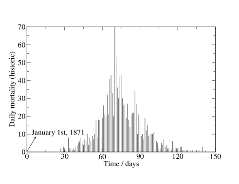
Figure 5: Daily mortality cases in the police district 14 (see Fig. 2) corresponding to the quarter San Telmo [6], $t=0$ corresponds to January 1, 1871.

3.5 Revising the clinical development of yellow fever.

A YF epidemic outbreak happened in Buenos Aires, in 1870, developing about 200 cases [4] (the text is ambiguous on whether the cases are toxic or fatal). The epidemic outbreak was noticed by February 22 (first death), a sailor who left Rio de Janeiro (Brazil) on February 7, and presumably landed on February 17 (no cases of YF were reported on board of the Poitou —the boat).

This well documented case allows us to see the margins of tolerance that have to be exercised in taking medical information prepared for clinical use as statistical information. Assume, following Penna, that the sailor was exposed to YF before boarding in Rio de Janeiro, according to information in Table 1 collected from the Pan American Health Organization [17], adding incubation and viremic period, we have a range of 6–10 days, hence the sailor was close to the limit of his infectious period. He was not toxic, according to the MD on board who signed a certificate accepted by the sanitary authority. Yet, five days later, he was dying, making the remission plus toxic period of 5 days, shorter than the range of 7–12 days listed in Table 1 and substantially shorter than the 10–15 days (remission plus toxic) communicated in Ref. [16]. Shall we assume as precise the values reported in Ref. [16, 17] we would have to conclude that the disease was substantially different, at least in its clinical evolution, in 1871 as compared with present days.

In clinical studies performed during a YF epidemic on the Jos Plateau, Nigeria, Jones and Wilson [32] report a 45.6% overall mortality and a significant difference in the duration of the illness for fatal and non-fatal cases with averages of 6.4 and 17.8 days. Série et al. [33] reports for the 1960–1962 epidemic in Ethiopia a mortality ranging from 43% (Kouré) to 100% (Boloso) and 50% (Menéra) with a total duration of the clinic phase of the illness of 7.14, 2.14 and 4.5 days, respectively (weighted average of 4.6 days in 18 cases).

We must conclude that the extension of the toxic period preceding the death presents high variability. This variability may represent variability in the illness or in medical criteria. For example, Série [33] indicates that the 100% mortality found at the Boloso Hospital is associated to the admission criteria giving priority to the most severe cases. In correspondence with this extremely high mortality level, the survival period is the shortest registered. The minimum length of the clinical phase is of 10–14 days or 13–18 days, depending of the source (adding viremic, remission and toxic periods). We note that not only the toxic period of fatal cases must be shorter than the same period for non-fatal cases, but also the viremic period must be shorter in average, if all the pieces of data are consistent.

The time elapsed between the first symptoms and death is probably longer today than in 1871, since it, in part, reflects the evolution of medical knowledge. The hospitalization time is also rather arbitrary and changes with medical practices which do not reflect changes in the disease.

A rudimentary procedure to correct for this differences is to shift the simulated mortality some fixed time between 5 and 8 days (the difference between our 13 days guessed (Table 1) and the 4.5–6.4 reported for Africa [33, 32]). Such a procedure is not conceptually optimal, but it is as much as it can be done within present knowledge. We certainly do not know whether just the toxic period must be shortened or the viremic period must be shortened as well, and in the latter case, how this would affect the spreading of the disease.

A second source of discrepancies between recorded data and simulations are the inaccuracies in the historic record. Can we consider the daily mortality record as a perfect account? Which was the protocol used to produce it? We can hardly expect it to be perfect, although we will not make any provision for this potential source of error.

4 Simulation results

The simulations were performed using a one-block spatial resolution, with the division in square blocks of the police districts 14 (San Telmo), 16, 2 and 4, corresponding to Concepción, Catedral Sur and Montserrat; and part of the districts 6, 18, 19, 19A and 20 (see Fig. 2), and totalized for each police district to obtain daily mortality comparable to those reported in Ref. [6] and picture in Fig. 5. Numerical mosquitoes were not allowed to fly over the river. At the remaining borders of the simulated region, a Stochastic Newmann Boundary Condition was used, meaning that the mosquito population of the next block across the boundary was considered equal to the block inside the region; but the number of mosquito dispersion events associated to the outside block was drawn randomly, independently of the events in the corresponding inner block. Larger regions for the simulations were tested producing no visible differences.

The time step was set to the small value of $30$ s, avoiding the introduction of further complications in the program related to fast event rates for tiny populations [34], although an implementation of the method in Ref. [34], not relying on the smallness of the time step so heavily, is desirable for a production phase of the program.

Before we proceed to the comparison between the historic mortality records of the epidemic and the simulated results, we need to gain some understanding regarding the sensitivity of the simulations to the parameters guessed and the best forms of presenting these results. We performed a moderate set of computations, since the code has not been optimized for speed and it is highly demanding for the personal computers where it runs for several days. Here, we illustrate the main lessons learned in our explorations. Poor people, unable to buy large quantities of water, had to rely mostly on the cisterns and other forms of keeping rain water. Since 1852, when the population of Buenos Aires was about 76000 people, there was an important immigration flow, increasing the population to about 178000 people by 1869 [7]. The immigrants occupied large houses where they rented a room, usually for an entire family, a housing that was known as “conventillo” and was the dominant form of housing in some districts such as San Telmo, where the epidemic started [20]. In some police chronicles of the time, houses with as many as 300 residents are mentioned [35]. Under such difficult social circumstances, we can only imagine that the number of breeding sites available to mosquitoes has to be counted as orders of magnitude larger than present-day available sites.

An a-priori and conservative estimation is to consider about ten times the number of breeding sites estimated today. Thus, we assume, as a first guess, 300 breeding sites per block in San Telmo. We will have to tune this number later as it regulates mosquito populations and the development of the epidemic focus. The number of breeding sites is the only parameter tuned to the results in this work.

More precisely, the criteria adopted was to make the number of (normalized) BS proportional to the number of houses per block taken from historic records [21], adjusting the proportionality factor to the observed dynamics. We introduce the notation BSxY to indicate a multiplicative factor of Y.

The population of each police district was set to the density values reported in the 1869 census [7, 21] and the police districts geography was taken from police records [36] and referenced according to maps of the city at the time [37, 38, 39, 40].

Table 2 shows the average population per block, initially estimated number of breeding sites and number of houses for the district of the initial focus, San Telmo #14 and nearby districts (# 16, 4, 2). A sketch of Buenos Aires police districts according to a 1887 map [37] is displayed alongside with the computer representation in Fig. 2.

It is a known feature of stochastic epidemic models [41] that the distribution of totals of infected people has two main contributions. One is that the small epidemic outbreaks when none or a few secondary cases are produced and the extinction time of the outbreak comes quickly. The otheris that the large epidemic outbreaks which, if the basic reproductive number is large enough, present a Gaussian shape separated by a valley of improbable epidemic sizes from the small outbreaks.

While the present model does not fall within the class of models discussed in Ref. [41], the general considerations applied to stochastic SIR models qualitatively apply to the present study. Yet, simulations started early during the summer season follow the pattern just described in Ref. [41], but simulations started later do not present the probability valley between large and small epidemics.

We have found useful to present the results disaggregated in the form: epidemic size, daily percentage of mortality relative to the total mortality and time to achieve half of the final mortality. This presentation will let us realize that most of the fluctuation is concentrated in the total epidemic size, while the daily evolution is relatively regular, except, perhaps, in the time taken to develop up to 50% of the mortality (depending on the abundance of vectors and the initial number of infected humans and chance).

4.1 Total mortality (epidemic size)

Since historical records include mostly the number of causalities, it appears sensible for the purposes of this study to use the total number of deaths as a proxy statistics for epidemic size.

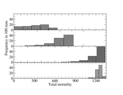
Figure 6: San Telmo. Total mortality histograms for different number of breeding sites, computed after 100 simulations with the same initial condition corresponding to 2 infectious people located in San Telmo on January 1, 1871, at the same location where the initial death happened in the historical event. From top to bottom, multiplication factors (bin-width : frequency of no-epidemic) BSx1 (126.2 : 0.23), BSx2 (209.8 : 0.09), BSx3 (128.2 : 0.06) and BSx4 (50.6 : 0.02). The y-axis indicates frequency in a set of 100 simulations.

The total mortality depends strongly on the stochastic nature of the simulations, initial conditions and ecological parameters guessed. Qualitatively, the results agree with the intuition, although this is an a-posteriori statement, i.e., only after seeing the results we can find intuitive interpretations for them.

The discussion assumes that the development of the epidemic outbreak was regulated by either the availability of vectors (mosquitoes) or the exhaustion of susceptible people, the first situation represents a striking difference with standard SIR models without seasonal dependence of the biological parameters. Actually, in Fig. 6, we compare frequencies of epidemics binned in five bins by final epidemic size for different sets of 100 simulations with different number of breeding sites. The number of breeding sites is varied in the same form all along the city, keeping the proportionality with housing, and it is expressed as multiplicative factor (BSx1=1, BSx2=2, BSx3=3, BSx4=4) presented in Table 2. Notice also that the width of the bins progresses as 126.2, 209.8, 128.2 and 50.6 indicating how the dispersion of final epidemic sizes first increases with the number of breeding sites but for larger numbers decreases.

We can see how for a factor 2 (BSx2) (and larger) the mortality saturates, indicating the epidemic outbreaks are limited by the number of susceptible people. For our original guess, factor 1, the epidemic is limited by the seasonal presence/absence of vectors. However, for higher factors, there is a substantial increase in large epidemic outbreaks with larger probabilities for larger epidemics. Only for the factor 4 (BSx4) the most likely bin includes the historical value of 1274 deaths.

A second feature, already shown in the Dengue model [10], is that outbreaks starting with the arrival of infectious people in late spring will have a lesser chance to evolve into a major epidemic. Yet, those that by chance develop are likely to become large epidemic outbreaks since they have more time to evolve. On the contrary, outbreaks started in autumn will have low chances to evolve and not a large number of casualties. The corresponding histograms can be seen in Fig. 7. Figure 7 also shows how the outbreaks that begin on December 16, as well as simulations starting on January 1, present higher probabilities of large epidemics than of small epidemics, but this tendency is reverted in simulations of outbreaks that start by February 16. This transition is, again, the transition between outbreaks regulated by the number of available susceptible humans and those regulated by the presence or absence of vectors.

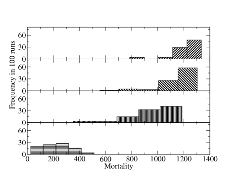
Figure 7: San Telmo. Total mortality histograms for different date of arrival of infectious people. Computed after 100 simulations with the same initial condition corresponding to 2 infectious people located in San Telmo and a density factor BSx2.5. From top to bottom: December 16, 1870; January 1, January 16 and February 15, 1871.

4.2 Mortality progression

One of the most remarkable facts unveiled by the simulations is that when the time evolution of the mortality is studied as a fraction of the total mortality, much of the stochastic fluctuations are eliminated and the curves present only small differences (see Fig. 8). The similarity of the normalized evolution allows us to focus on the time taken to produce half of the mortality (labelled $T_{1/2}$).

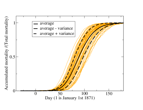
Figure 8: Evolution of the mortality level for all the epidemics with three or more fatal cases in a batch of 100 simulations (96 runs) differing only in the pseudo-random series. The breeding sites number has a factor 4, and the initial contagious people were placed on January 1, 1871, in San Telmo.

We notice, in Fig. 8, that the $T_{1/2}$ in these runs lay between 69–110, compared to the historic values of $T_{1/2}=$73.

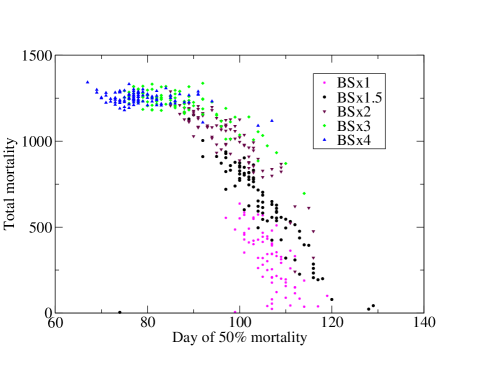
Figure 9: San Telmo. Total mortality versus day when the mortality reached half its final number for different number of breeding sites. The mortality appears to be mainly a function of $T_{1/2}$ and roughly independent of the number of breeding sites.

The latter observation brings the attention to a remarkable fact of the simulations: not only the normalized progression of the outbreaks are rather similar but also, there is a correspondence between early development and large mortality. Drawing $T_{1/2}$ against total-mortality (Fig. 9), we see that even for different number of breeding sites, all the simulations indicate that the final size is a noisy function of the day when the mortality reaches half its final value. This function is almost constant for small $T_{1/2}$ and becomes linear with increasing dispersion when $T_{1/2}$ is relatively large. Once again, the two different forms the outbreak is controlled.

5 Real against simulated epidemic

We would like to establish the credibility of the statement: the historic mortality record for the San Telmo focus belongs to the statistics generated by the simulations.

To achieve this goal, we need to compare the daily mortality in the historical record and the simulations. Since, in the model, the mortality proceeds day after day with independent random increments (as a consequence of the Poisson character of the model), it is reasonable to consider the statistics

$$\chi^{2}=\sum_{i}\left(\frac{HM(i)-MM(i)}{D(i)}\right)^{2}$$ (2)

where $i$ runs over the days of the year, $HM(i)$ is the fraction of the total death toll in the historic record for the day $i$, $MM(i)$ is the average of the same fraction obtained in the simulations and $D(i)$ is the corresponding standard deviation for the simulations. The sum runs over the number of days in which the variance is not zero, for BSx3 and BSx4 in no case $D(i)=0$ and $(HM(i)-MM(i)\neq 0)$. The number of degrees corresponds to the number of days with non-zero mortality in the simulations minus one. The degree discounted accounts for the fact that $\sum_{i}HM(i)=\sum_{i}MM(i)=1$.

5.1 Tuning of the simulations

Before we proceed, we have to find an acceptable number of breeding sites, a reasonable day for the arrival of infected individuals (assumed to be 2 individuals arbitrarily) and adjust for the uncertainty in survival time. Actually, moving the day of arrival $d$ days earlier and shortening the survival time by $d$ will have essentially the same effect on the simulated mortality (providing $d$ is small), which is to shift the full series by $d$ days. This is, assigning to the day $i$ the simulated mortality $SM$ of the day $i+d$, ($SM(i+d)$). Hence, only two of the parameters will be obtained from this data.

BSxY	d	$\chi^{2}$	degree	Probability
2	8	490.2	177	0.
3	7	191.7	173	0.15
4	3	151.9	168	0.80
4	4	143.8	168	0.91
4	5	145.6	168	0.89

Table 3: $\chi^{2}$ calculations according to (2). We indicate the multiplicative factor applied to the breeding sites described in Table 2, the shift applied to the statistics produce with the parameters of Table 1, the value of the statistic $\chi^{2}$, the number of degrees of freedom, and the probability $P(x>\chi^{2})$ for a random variable $x$ distributed as a $\chi^{2}$-distribution with the indicated degrees of freedom. The standard reading of the $\chi^{2}$ test indicates that, for BSx3 and BSx4, the statement “the deviations from the simulations mean of the historic record (deviations assumed to be distributed as $\chi^{2}$ with the indicated degrees) belong to the simulated set” is not found likely to be false by the test in the cases BSx3 and BSx4.

As we have previously observed, the total mortality presents a large variance in the simulations. Moreover, in medical accounts of modern time [32, 33], the mortality ranges between $46\%$ and $100\%$ while in historical accounts the percentage goes from $20$ to $70$ [23]. Hence, a simple adjustment of the mortality coefficient from our arbitrary $50\%$ within such a wide range would suffice to eliminate the contributions of the total epidemic size. The average simulated epidemic for BSx4 is of $\approx 1248$ deaths while the historic record is of $1274$ deaths. Hence, to match the mean with the historic record, it would suffice to correct the mortality from $50\%$ to $51\%$.

We can disregard the idea that the epidemic started before December 20, 1870 (Penna’s conjecture), since it is not possible to simultaneously obtain an acceptable final mortality and an acceptable evolution of the outbreak. Our best attempt corresponds to an epidemic starting by December 14, 1870, which averages $\approx 1212$ deaths and with a deviation of the mortality of $\chi^{2}=219.1$ with 175 degrees, giving a probability $P(x\geq 219,1)=0.01$.

We focus on arrival dates around January 1, 1871. We can also disregard, for this initial condition, the original guess BSx1 corresponding to 300 breeding sites per block in San Telmo, since it produces too small epidemics. We present results for the epidemics corresponding to BSx2, BSx3 and BSx4 in Table 3 for different numbers of BS and shift $d$.

5.2 Comparison

The conclusion of the $\chi^{2}$ tests is that the simulations performed with BSx3 and beginning between December 24 1870 and January 1, 1871 (with a survival period shortened between 0 and 8 days) are compatible with the historical record. However, the compatibility is larger when BSx4 is considered and the beginning of the epidemic is situated between December 28, 1870 and January 5, 1871 (with a survival period shortened between 0 and 8 days respectively). We illustrate this comparison with Fig. 10.

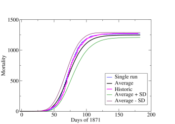
Figure 10: The historic record of accumulated mortality as a function of the day of the year 1871 is presented. The averaged accumulated mortality as well as curves shifted one standard deviation are shown for comparison. An acceptable look alike individual simulation chose by visual inspection from a set of 100 simulations is included as well. Two exposed individuals (not yet contagious) were introduced in the same blocks where the historic epidemic started the day January 1, 1871, with BSx4. The simulated mortality is anticipated in 4 days. Statistical estimates were taken as averages over 96 runs which resulted in secondary mortality, out of a set of 100 runs.

5.3 The 1870 outbreak

The records for the 1870 outbreak are scarce. Of the recognized cases, only 32 entered the Lazareto (hospital) and 19 of them were originated in the same block that the first case. Secondary cases are registered at the Lazareto’ books starting on March 30 (two cases) and continuing with daily cases. the final outcome of these cases and the cases not entered at the Lazareto [4] are not clear.

Except for the precise initial condition, corresponding to one viremic (infective) person located at the Hotel Roma (district 4 in Fig. 2), the information is too imprecise to produce a demanding test for the model.

We performed a set of 100 simulations introducing one viremic (infective) person at the precise block where the Hotel Roma was, on February 17. The number of breeding sites was kept at the same factor 4 with respect to the values tabulated in Table 2 that was used for the best results in the study of the 1871 outbreak. Needless to say, this does not need to be true, as the number of breeding sites may change from season to season.

The distribution of the final mortality is shown in Fig. 11. As we can see, relatively small epidemics of less than 200 deaths cannot be ruled out, although there are much larger epidemics also likely to happen.

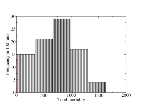
Figure 11: Mortality distribution for the simulations beginning on February 17 with the incorporation of one infective (viremic) in the block of the Hotel Roma and BSx4. The histogram is the result of 87 runs which resulted in epidemics (13 runs did not result in epidemics). The width of the bins is 322.2, and the first epidemic bin goes from 17 to 339 deaths with a frequency of 15/100.

Actually, a slow start of the epidemic outbreak would favor a small final mortality, as it can be seen in Fig. 12. Not only there is a relation between a low mortality early during the outbreak (such as April 15) and the final mortality, but we also see that the sharp division between small and large epidemics is not present in this family of epidemic outbreaks differing only in the pseudo-random number sequence.

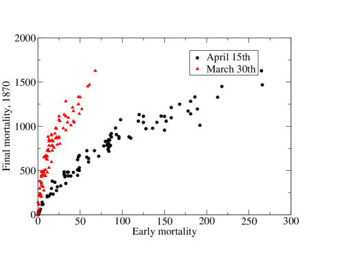
Figure 12: Final mortality against early mortality for two dates: March 30 and April 15. A low early mortality “predicts” a low final mortality as the outbreak does not have enough time to develop. Simulations correspond to the conditions of the 1870 small epidemic. BSx4, one infected arriving to the Hotel Roma on February 17. The historic information indicates that secondary cases were recorded by March 30. Hence, corresponding to a slow start. The final mortality is not known, but it is believed it has been in the 100–200 range.

For the smallest epidemics simulated, the secondary mortality starts after March 30. Hence, the 1870 focus can be understood as a case of relative good luck and a late start within more or less the same conditions than the outbreak of 1871.

6 Conclusions and final discussion

In this work, we have studied the development of the initial focus in the YF epidemic that devastated Buenos Aires (Argentina) in 1871 using methods that belong to complex systems epistemology [42].

The core of the research performed has been the development of a model (theory) for an epidemic outbreak spread only by the mosquito Aedes aegypti represented according to current biological literature such as Christophers [2] and others. The translation of the mosquito’s biology into a computer code has been performed earlier [8, 9] and the basis for the spreading of a disease by this vector has been elaborated in the case of Dengue previously [10]. The present model for YF is then an adaptation of the Dengue model to the particularities of YF, and the present attempt of validation (failed falsification) reflects also on the validity of this earlier work.

The present study owes its existence to the work of anonymous police officers [6] that gathered and recorded epidemics statistics during the epidemic outbreak, in a city that was not only devastated by the epidemic, but where the political authorities left in the middle of the drama as well [20].

We have gathered (and implemented in a model) entomological, ecological and medical information, as well as geographic, climatological and social information. After establishing the historical constraints restricting our attempts to simulate the historical event, we have adjusted the density of breeding sites to be the equivalent to 1200 half-liter pots as those encountered in today Buenos Aires cemeteries (the number corresponds to San Telmo quarter). Perhaps a better idea of the number of mosquitoes present is given by the maximum of the average number of bites per person per day estimated by the model, which results in 5 bites/(person day) (to be precise: the ratio between the maximum number of bites in a block during a week and the population of the block, divided by seven).

The population of the domestic mosquito Aedes aegypti in Buenos Aires 1870–1871 was large enough to almost assure the propagation of YF during the summer season. The only effective measures preventing the epidemic were the natural quarantine resulting from the distance to tropical cities were YF was endemic (such as Rio de Janeiro) and the relatively small window for large epidemics, since the extinction of the adult form of the mosquito during the winter months prevents the overwintering of YF. In this sense, the relatively small outbreak of 1870 is an example of how a late arrival of the infected individual combined with a touch of luck produced only a minor sanitary catastrophe.

By 1871, as a consequence of the end of the Paraguayan war and the emergence of YF in Asunción, the conditions for an almost unavoidable epidemic in Buenos Aires were given. The intermediate step taken in Corrientes, with the panic and partial evacuation of the city, adding the lack of quarantine measures, was more than enough to make certain the epidemic in Buenos Aires. On the contrary, Penna’s conjecture of an earlier starting during December, 1870 are inconsistent with the biological and medical times as implemented in the model. We can disregard this conjecture as highly improbable.

The historic mortality record is consistent with an epidemic starting between December 28 and January 5, being the symptomatic period (viremic plus remission plus toxic) of the illness between 13 and 5 days. Furthermore, the existence of non-fatal cases of YF by January 6 mentioned by some sources [19] would be consistent, provided the cases were imported.

In retrospect, the present research began as an attempt to validate/falsificate the YF model and, in more general terms, the model for the transmission of viral diseases by Aedes aegypti using the historic data of this large YF epidemic. As the research progressed, it became increasingly evident that the model was robust. In successive attempts, every time the model failed to produce a reasonable result, it forced us to revise the epidemiological and historical hypotheses. In these revisions, we ended up realizing that the accepted origin of the epidemic in imported cases from Brazil, actually hides the central role that the epidemics in Corrientes had, and the gruesome failure of not quarantining Corrientes once the mortality started by December 16, 1870, about two weeks before the deducted beginning of the outbreak in Buenos Aires.

The same study of inconsistencies between the data and the reconstruction made us focus on the survival time of those clinically diagnosed with YF that finally die. The form in which the illness evolves anticipates the final result. Jones and Wilson [32] indicate the symptoms of cases with a bad prognosis including the rapidity and degree of jaundice. This information suggests, in terms of modeling, that death is not one of two possible outcomes at the end of the “toxic period”, as we have first thought. Separation of to-recover and to-die subpopulations could (should?) be performed earlier in the development of the illness, each subpopulation having its own parameters for the illness. Yet, while in theory this would be desirable, in practice it would have, for the time being, no effect, since the characteristic periods of the illness have not been measured in these terms.

Epidemics transmitted by vectors come to an end either when the susceptible population has been sufficiently exposed so that the replication of the virus is slowed down (the classical consideration in SIR models) or when the vector’s population is decimated by other (for example, climatic) reasons. The model shows that both situations can be distinguished in terms of the mortality statistics.

We have also shown that the total mortality of the epidemic is not difficult to adjust by changing the death probability of the toxic phase, and as such, it is not a demanding test for a model. The daily mortality, when normalized, shows sensitivity to the mosquito abundance, specially in the evolution times involved, since the general qualitative shape appears to be fixed. In particular, the date in which the epidemic reaches half the total mortality is advanced by larger mosquito populations. However, only comparison of the simulated and historical daily mortality put enough constraints to the free data in the model (date of arrival of infected people and mosquito population) to allow for a selection of possible combinations of their values.

As successful as the model appears to be, it is completely unable to produce the total mortality in the city, or the spatial extension of the full epidemic. The simulations produce with BSx4 less than 4500 deaths, while in the historic record, the total mortality in the city is above 13000 cases. The historical account, and the recorded data, show that after the initial San Telmo focus has developed, a second focus in the police district 13 (see Fig. 2) developed, shortly several other foci developed that could not be tracked [4]. Unless the spreading of the illness by infected humans is introduced (or some other method to make long jumps by the illness), such events cannot be described. It is worth noticing that the mobility patterns in 1871 are expected to be drastically different from present patterns, and as such, the application of models with human mobility [43] is not straightforward and requires a historical study.

One of the most important conclusions of this work is that the logical consistency of mathematical modeling puts a limit to ad-hoc hypotheses, so often used in a-posteriori explanations, as it forces to accept not just the desired consequence of the hypotheses, but all other consequences as well.

Last, eco-epidemiological models are adjusted to vector populations pre-existing the actual epidemics and can therefore be used in prevention to determine epidemic risk and monitor eradication campaigns. In the present work, the tuning was performed in epidemic data only because it is actually impossible to know the environmental conditions more than one hundred years ago. Yet, our wild initial guess for the density of breeding sites resulted sufficiently close to allow further tuning.

Appendix A Appendix

A.1 Populations and events of the stochastic transmission model

We consider a two dimensional space as a mesh of squared patches where the dynamics of vectors, hosts and the disease take place. Only adult mosquitoes, Flyers, can fly from one patch to a next one according to a diffusion-like process. The coordinates of a patch are given by two indices, $i$ and $j$, corresponding to the row and column in the mesh. If $X_{k}$ is a subpopulation in the stage $k$, then $X_{k}(i,j)$ is the $X_{k}$ subpopulation in the patch of coordinates $(i,j)$.

Population of both hosts (Humans) and vectors (Aedes aegypti) were divided into subpopulations representing disease status: SEI for the vectors and SEIrRTD for the human population.

Ten different subpopulations for the mosquito were taken into account, three immature subpopulations: eggs $E_{(i,j)}$, larvae $L_{(i,j)}$ and pupae $P_{(i,j)}$, and seven adult subpopulations: non parous adults $A1_{(i,j)}$, susceptible flyers $Fs_{(i,j)}$, exposed flyers $Fe_{(i,j)}$, infectious flyers $Fi_{(i,j)}$ and parous adults in the three disease status: susceptible $A2s_{(i,j)}$, exposed $A2e_{(i,j)}$ and infectious $A2i_{(i,j)}$.

The $A1_{(i,j)}$ is always susceptible, after a blood meal it becomes a flyer, susceptible $Fs_{(i,j)}$ or exposed $Fe_{(i,j)}$, depending on the disease status of the host. If the host is infectious, $A1_{(i,j)}$ becomes an exposed flyer $Fe_{(i,j)}$ but if the host is not infectious, then the $A1_{(i,j)}$ becomes a susceptible flyer $Fs_{(i,j)}$. The transmission of the virus depends not only on the contact between vector and host but also on the transmission probability of the virus. In this case, we have two transmission probabilities: the transmission probability from host to vector $ahv$ and the transmission probability from vector to host $avh$.

Human population $Nh_{(i,j)}$ was split into seven different subpopulations according to the disease status: susceptible humans $Hs_{(i,j)}$, exposed humans $He_{(i,j)}$, infectious humans $Hi_{(i,j)}$, humans in remission state $Hr_{(i,j)}$, toxic humans $Ht_{(i,j)}$, removed humans $HR_{(i,j)}$ and dead humans because of the disease $Hd_{(i,j)}$.

The evolution of the seventeen subpopulations is affected by events that occur at rates that depend on subpopulation values and some of them also on temperature, which is a function of time since it changes over the course of the year seasonally [8, 9].

A.2 Events related to immature stages

Table 4 summarizes the events and rates related to immature stages of the mosquito during their first gonotrophic cycle. The construction of the transition rates and the election of model parameters related to the mosquito biology such as: $me$ mortality of eggs, $elr$ hatching rate, $ml$ mortality of larvae, $\alpha$ density-dependent mortality of larvae, $lpr$ pupation rate, $mp$: mortality of pupae, $par$ pupae into adults development coefficient and the $ef$ emergence factor were described in detail previously [8, 9].

Event	Effect	Transition rate
Egg death	$E_{(i,j)}\rightarrow E_{(i,j)}-1$	$me\times E_{(i,j)}$
Egg hatching	$E_{(i,j)}\rightarrow E_{(i,j)}-1$ $L_{(i,j)}\rightarrow L_{(i,j)}+1$	$elr\times E_{(i,j)}$
Larval death	$L_{(i,j)}\rightarrow L_{(i,j)}-1$	$ml\times L_{(i,j)}+\alpha\times L_{(i,j)}\times(L_{(i,j)}-1)$
Pupation	$L_{(i,j)}\rightarrow L_{(i,j)}-1$ $P_{(i,j)}\rightarrow P_{(i,j)}+1$	$lpr\times L_{(i,j)}$
Pupal death	$P_{(i,j)}\rightarrow P_{(i,j)}-1$	$(mp+par\times(1-(ef/2)))\times P_{(i,j)}$
Adult emergence	$P_{(i,j)}\rightarrow P_{(i,j)}-1$ $A1_{(i,j)}\rightarrow A1_{(i,j)}+1$	$par\times(ef/2)\times P_{(i,j)}$

Table 4: Event type, effects on the populations and transition rates for the developmental model. The coefficients are $me$: mortality of eggs; $elr$: hatching rate; $ml$: mortality of larvae; $\alpha$: density-dependent mortality of larvae; $lpr$: pupation rate; $mp$: mortality of pupae; $par$: pupae into adults development coefficient; $ef$: emergence factor. The values of the coefficients are available in subsections A.6 and A.7.

The natural regulation of Aedes aegypti populations is due to intra-specific competition for food and other resources in the larval stage. This regulation was incorporated into the model as a density-dependent transition probability which introduces the necessary nonlinearities that prevent a Malthusian growth of the population. This effect was incorporated as a nonlinear correction to the temperature dependent larval mortality.

Then, larval mortality can be written as: $mlL_{(i,j)}+\alpha L_{(i,j)}\times(L_{(i,j)}-1)$ where the value of $\alpha$ can be further decomposed as $\alpha=\alpha_{0}/\text{BS}_{(i,j)}$ with $\alpha_{0}$ being associated with the carrying capacity of one (standardised) breeding site and $\text{BS}_{(i,j)}$ being the density of breeding sites in the $(i,j)$ patch [8, 9].

A.3 Events related to the adult stage

Aedes aegypti females ($A1$ and $A2$) require blood to complete their gonotrophic cycles. In this process, the female may ingest viruses with the blood meal from an infectious human during the human Viremic Period $VP$. The viruses develop within the mosquito during the Extrinsic Incubation Period $EIP$ and then are reinjected into the blood stream of a new susceptible human with the saliva of the mosquito in later blood meals. The virus in the exposed human develops during the Intrinsic incubation Period $IIP$ and then begin to circulate in the blood stream (Viremic Period), the human becoming infectious. The flow from susceptible to exposed subpopulations (in the vector and the host) depends not only on the contact between vector and host but also on the transmission probability of the virus. In our case, there are two transmission probabilities: the transmission probability from host to vector $ahv$ and the transmission probability from vector to host $avh$.

Event	Effect	Transition rate
Adults 1 Death	$A1_{(i,j)}\rightarrow A1_{(i,j)}-1$	$ma\times A1_{(i,j)}$
I Gonotrophic cycle with virus exposure	$A1_{(i,j)}\rightarrow A1_{(i,j)}-1$ $Fe_{(i,j)}\rightarrow Fe_{(i,j)}+1$	$cycle1\times A1_{(i,j)}\times(Hi_{(i,j)}/Nh_{(i,j)})\times ahv$
I Gonotrophic cycle without virus exposure	$A1_{(i,j)}\rightarrow A1_{(i,j)}-1$ $Fs_{(i,j)}\rightarrow Fs_{(i,j)}+1$	$cycle1\times A1_{(i,j)}\times((((Nh_{(i,j)}-Hi_{(i,j)})/Nh_{(i,j)})+(1-ahv)\times(Hi_{(i,j)}/Nh_{(i,j)}))$
Oviposition of susceptible flyers	$E_{(i,j)}\rightarrow E_{(i,j)}+egn$ $Fs_{(i,j)}\rightarrow Fs_{(i,j)}-1$ $A2s_{(i,j)}\rightarrow A2s_{(i,j)}+1$	$ovr_{(i,j)}\times Fs_{(i,j)}$
Oviposition of exposed flyers	$E_{(i,j)}\rightarrow E_{(i,j)}+egn$ $Fe_{(i,j)}\rightarrow Fe_{(i,j)}-1$ $A2e_{(i,j)}\rightarrow A2e_{(i,j)}+1$	$ovr_{(i,j)}\times Fe_{(i,j)}$
Oviposition of infected flyers	$E_{(i,j)}\rightarrow E_{(i,j)}+egn$ $Fi_{(i,j)}\rightarrow Fi_{(i,j)}-1$ $A2i_{(i,j)}\rightarrow A2i_{(i,j)}+1$	$ovr_{(i,j)}\times Fi_{(i,j)}$

Table 5: Event type, effects on the subpopulations and transition rates for the developmental model. The coefficients are $ma$: mortality of adults; $cycle1$: gonotrophic cycle coefficient (number of daily cycles) for adult females in stages $A1$.; $ahv$: transmission probability from host to vector; $ovr_{(i,j)}$: oviposition rate by flyers in the (i,j) patch; $egn$: average number of eggs laid in an oviposition. The values of the coefficients are available in Table 1, subsections A.6, A.7, A.8 and A.9.

The events related to the adult stage are shown in Table 5 to 8. Table 5 summarizes the events and rates related to adults during their first gonotrophic cycle and related to oviposition by flyers according to their disease status.

Event	Effect	Transition rate
II Gonotrophic cycle of susceptible Adults 2 with virus exposure	$A2s_{(i,j)}\rightarrow A2s_{(i,j)}-1$ $Fe_{(i,j)}\rightarrow Fe_{(i,j)}+1$	$cycle2\times A2s_{(i,j)}\times(Hi_{(i,j)}/Nh_{(i,j)})\times ahv$
II Gonotrophic cycle of susceptible Adults 2 without virus exposure	$A2s_{(i,j)}\rightarrow A1_{(i,j)}-1$ $Fs_{(i,j)}\rightarrow Fs_{(i,j)}+1$	$cycle2\times A2s_{(i,j)}\times((((Nh_{(i,j)}-Hi_{(i,j)})/Nh_{(i,j)})+(1-ahv)\times(Hi_{(i,j)}/Nh_{(i,j)}))$
II Gonotrophic cycle of exposed Adults 2	$A2e_{(i,j)}\rightarrow A2e_{(i,j)}-1$ $Fe_{(i,j)}\rightarrow Fe_{(i,j)}+1$	$cycle2\times A2e_{(i,j)}$

Table 6: Event type, effects on the subpopulations and transition rates for the developmental model. The coefficients are $cycle2$: gonotrophic cycle coefficient (number of daily cycles) for adult females in stages $A2$.; $ahv$: transmission probability from host to vector. The values of the coefficients are available in Table 1, subsections A.6, A.7, A.8 and A.9.

Table 6 and Table 7 summarize the events and rates related to adult 2 gonotrophic cycles, exposed Adults 2 and exposed flyers becoming infectious and human contagion.

Event	Effect	Transition rate
Exposed Adults 2 becoming infectious	$A2e_{(i,j)}\rightarrow A2e_{(i,j)}-1$ $A2i_{(i,j)}\rightarrow A2i_{(i,j)}+1$	$(1/(EIP-(1/ovr_{(i,j)})))A2e_{(i,j)}$
Exposed flyers becoming infectious	$Fe_{(i,j)}\rightarrow Fe_{(i,j)}-1$ $Fi_{(i,j)}\rightarrow Fi_{(i,j)}+1$	$(1/(EIP-(1/ovr_{(i,j)})))Fe_{(i,j)}$
II Gonotrophic cycle of infectious Adults 2 without human contagion	$A2i_{(i,j)}\rightarrow A2i_{(i,j)}-1$ $Fi_{(i,j)}\rightarrow Fi_{(i,j)}+1$ $Hs_{(i,j)}\rightarrow Hs_{(i,j)}-1$ $He_{(i,j)}\rightarrow He_{(i,j)}+1$	$cycle2\times A2i_{(i,j)}\times(Hs_{(i,j)}/Nh_{(i,j)})\times avh$
II Gonotrophic cycle of infectious Adults 2 without human contagion	$A2i_{(i,j)}\rightarrow A2i_{(i,j)}-1$ $Fi_{(i,j)}\rightarrow Fi_{(i,j)}+1$	$cycle2\times A2i_{(i,j)}\times((((Nh_{(i,j)}-Hs_{(i,j)})/Nh_{(i,j)})+(1-avh)\times(Hs_{(i,j)}/Nh_{(i,j)}))$

Table 7: Event type, effects on the subpopulations and transition rates for the developmental model. The coefficients are $cycle2$: gonotrophic cycle coefficient (number of daily cycles) for adult females in stages $A2$; $ovr_{(i,j)}$: oviposition rate by flyers in the $(i,j)$ patch; $avh$: transmission probability from vector to host; $EIP$: extrinsic incubation period. The values of the coefficients are available in Table 1, subsections A.6, A.7, A.8 and A.9

Table 8 summarizes the events and rates related to non parous adult (Adult 2) and Flyer death.

Event	Effect	Transition rate
Susceptible flyer Death	$Fs_{(i,j)}\rightarrow Fs_{(i,j)}-1$	$ma\times Fs_{(i,j)}$
Exposed flyer Death	$Fe_{(i,j)}\rightarrow Fe_{(i,j)}-1$	$ma\times Fe_{(i,j)}$
Infectious flyer Death	$Fi_{(i,j)}\rightarrow Fi_{(i,j)}-1$	$ma\times Fi_{(i,j)}$
Susceptible Adult 2 Death	$A2s_{(i,j)}\rightarrow A2s_{(i,j)}-1$	$ma\times A2s_{(i,j)}$
Exposed Adult 2 Death	$A2e_{(i,j)}\rightarrow A2e_{(i,j)}-1$	$ma\times A2e_{(i,j)}$
Infectious Adult 2 Death	$A2i_{(i,j)}\rightarrow A2i_{(i,j)}-1$	$ma\times A2i_{(i,j)}$

Table 8: Event type, effects on the subpopulations and transition rates for the developmental model. The coefficients are $ma$: adult mortality. The values of the coefficients are available in subsection A.7

A.4 Events related to flyer dispersal

Some experimental results and observational studies show that the Aedes aegypti dispersal is driven by the availability of oviposition sites [44, 45, 46]. According to these observations, we considered that only the Flyers $F_{(i,j)}$ can fly from patch to patch in search of oviposition sites. The implementation of flyer dispersal has been described elsewhere [9].

The general rate of the dispersal event is given by: $\beta\times F_{(i,j)}$, where $\beta$ is the dispersal coefficient and $F_{(i,j)}$ is the Flyer population which can be susceptible $Fs_{(i,j)}$, exposed $Fe_{(i,j)}$ or infectious $Fi_{(i,j)}$ depending on the disease status.

The dispersal coefficient $\beta$ can be written as

$$\beta=\left\{\begin{array}[]{cc}0&\mbox{\footnotesize if the patches are disjoint}\\ diff/d_{ij}^{2}&\mbox{\footnotesize if the patches have}\\ &\mbox{\footnotesize at least a common point}\end{array}\right.$$ (3)

where $d_{ij}$ is the distance between the centres of the patches and $diff$ is a diffusion-like coefficient so that dispersal is compatible with a diffusion-like process [9].

A.5 Events related to human population

Event	Effect	Transition rate
Born of susceptible humans	$Hs_{(i,j)}\rightarrow Hs_{(i,j)}+1$	$mh\times Nh_{(i,j)}$
Death of susceptible humans	$Hs_{(i,j)}\rightarrow Hs_{(i,j)}-1$	$mh\times Hs_{(i,j)}$
Death of exposed humans	$He_{(i,j)}\rightarrow He_{(i,j)}-1$	$mh\times He_{(i,j)}$
Transition from exposed to viraemic	$He_{(i,j)}\rightarrow He_{(i,j)}-1$ $Hi_{(i,j)}\rightarrow Hi_{(i,j)}+1$	$(1/IIP)\times He_{(i,j)}$
Death of Infectious humans	$Hi_{(i,j)}\rightarrow Hi_{(i,j)}-1$	$mh\times Hi_{(i,j)}$
Transition from infectious humans to humans in remission state	$Hi_{(i,j)}\rightarrow Hi_{(i,j)}-1$ $Hr_{(i,j)}\rightarrow Hr_{(i,j)}+1$	$(1/VP)\times Hi_{(i,j)}$
Death of humans in remission state	$Hr_{(i,j)}\rightarrow Hr_{(i,j)}-1$	$mh\times Hr_{(i,j)}$
Transition from humans in remission to toxic humans	$Hr_{(i,j)}\rightarrow Hr_{(i,j)}-1$ $Ht_{(i,j)}\rightarrow Ht_{(i,j)}+1$	$((1-rar)/rP)\times Hr_{(i,j)}$
Recovery of humans in remission	$Hr_{(i,j)}\rightarrow Hr_{(i,j)}-1$ $HR_{(i,j)}\rightarrow HR_{(i,j)}+1$	$(rar/rP)\times Hr_{(i,j)}$
Death of removed humans	$HR_{(i,j)}\rightarrow HR_{(i,j)}-1$	$mh\times HR_{(i,j)}$
Death of toxic humans	$Ht_{(i,j)}\rightarrow Ht_{(i,j)}-1$ $Hd_{(i,j)}\rightarrow Hd_{(i,j)}+1$	$(mt/tP)\times Ht_{(i,j)}$
Recovery of toxic humans	$Ht_{(i,j)}\rightarrow Ht_{(i,j)}-1$ $HR_{(i,j)}\rightarrow HR_{(i,j)}+1$	$((1-mt)/tP)\times Ht_{(i,j)}$

Table 9: Event type, effects on the subpopulations and transition rates for the developmental model. The coefficients are $mh$: human mortality coefficient; $VP$: human viremic period; $mh$: human mortality coefficient; $IIP$: intrinsic incubation period; $rP$: remission period; $tP$: toxic period; $rar$: recovery after remission probability; $mt$: mortality probability for toxic patients. The values of the coefficients are available in Table 1.

Human contagion has been already described in Table 7. Table 9 summarizes the events and rates in which humans are involved. The human population was fluctuating but balanced, meaning that the birth coefficient was considered equal to the mortality coefficient $mh$.

A.6 Developmental Rate coefficients

The developmental rates that correspond to egg hatching, pupation, adult emergence and the gonotrophic cycles were evaluated using the results of the thermodynamic model developed by Sharp and DeMichele [47] and simplified by Schoofield et al. [48]. According to this model, the maturation process is controlled by one enzyme which is active in a given temperature range and is deactivated only at high temperatures. The development is stochastic in nature and is controlled by a Poisson process with rate $R_{D}(T)$. In general terms, $R_{D}(T)$ takes the form

$$R {}_{D}(T)=R_{D}(298\text{ K})$$ (4)

$$\times\frac{(T/298\text{ K})\exp((\Delta H_{A}/R)(1/298\text{ K}-1/T))}{1+\exp(\Delta H_{H}/R)(1/T_{1/2}-1/T))}$$

where $T$ is the absolute temperature, $\Delta H_{A}$ and $\Delta H_{H}$ are thermodynamics enthalpies characteristic of the organism, $R$ is the universal gas constant, and $T_{1/2}$ is the temperature when half of the enzyme is deactivated because of high temperature.

Table 10 presents the values of the different coefficients involved in the events: egg hatching, pupation, adult emergence and gonotrophic cycles. The values are taken from Ref. [30] and are discussed in Ref. [8].

Develop. Cycle (4)	$R_{D}(T)$	$R_{D}(298\text{ K})$	$\Delta H_{A}$	$\Delta H_{H}$	$T_{1/2}$
Egg hatching	elr	0.24	10798	100000	14184
Larval develop.	lpr	0.2088	26018	55990	304.6
Pupal Develop.	par	0.384	14931	-472379	148
Gonotrophic c. ($A1$)	cycle1	0.216	15725	1756481	447.2
Gonotrophic c. ($A2$)	cycle2	0.372	15725	1756481	447.2

Table 10: Coefficients for the enzymatic model of maturation [Eq. (4)]. $R_{D}$ is measured in day^-1, enthalpies are measured in (cal / mol) and the temperature $T$ is measured in absolute (Kelvin) degrees.

A.7 Mortality coefficients

Egg mortality.

The mortality coefficient of eggs is $me=0.01$ 1/day, independent of temperature in the range $278\text{ K}\leq T\leq 303\text{ K}$ [49].

Larval mortality.

The value of $\alpha_{0}$ (associated to the carrying capacity of a single breeding site) is $\alpha_{0}=1.5$, and was assigned by fitting the model to observed values of immatures in the cemeteries of Buenos Aires [8]. The temperature dependent larval death coefficient is approximated by $ml=0.01+0.9725\exp(-(T-278)/2.7035)$ and it is valid in the range $278\text{ K}\leq T\leq 303\text{ K}$ [50, 51, 52].

Pupal mortality.

The intrinsic mortality of a pupa has been considered as $mp=0.01+0.9725exp(-(T-278)/2.7035)$ [50, 51, 52]. Besides the daily mortality in the pupal stage, there is an additional mortality contribution associated to the emergence of the adults. We considered a mortality of $17\%$ of the pupae at this event, which is added to the mortality rate of pupae. Hence, the emergence factor is $ef=0.83$ [53].

Adult mortality.

Adult mortality coefficient is $ma=0.091/\text{day}$ and it is considered independent of temperature in the range $278\text{ K}\leq T\leq 303\text{ K}$ [50, 2, 54].

A.8 Fecundity and oviposition coefficient

Females lay a number of eggs that is roughly proportional to their body weight ($46.5\text{ eggs/mg}$) [55, 56]. Considering that the mean weight of a three-day-old female is $1.35\text{ mg}$ [2], we estimated the average number of eggs laid in one oviposition as $egn=63$.

The oviposition coefficient $ovr_{(i,j)}$ depends on breeding site density $\text{BS}_{(i,j)}$ and it is defined as:

$$ovr_{(i,j)}=\left\{\begin{array}[]{cccc}&\theta/tdep&\mbox{ if }&\text{BS}_{(i,j)}\leq 150\\ &1/tdep&\mbox{ if }&\text{BS}_{(i,j)}>150\end{array}\right.$$ (5)

where $\theta$ was chosen as $\theta=\text{BS}_{(i,j)}/150$, a linear function of the density of breeding sites [9].

A.9 Dispersal coefficient

We chose a diffusion-like coefficient of $diff$ = 830 m²/day which corresponds to a short dispersal, approximately a mean dispersal of 30 m in one day, in agreement with short dispersal experiments and field studies analyzed in detail in our previous article [9].

A.10 Mathematical description of the stochastic model

The evolution of the subpopulations is modeled by a state dependent Poisson process [57, 41] where the probability of the state:

$$(E,L,P, A1,A2s,A2e,A2i,Fs,Fe,Fi,$$

$$Hs,He,Hi,Hr,Ht,HR,Hd)_{(i,j)}$$

evolves in time following a Kolmogorov forward equation that can be constructed directly from the information collected in Tables 4 to 9 and in Eq. 3.

A.11 Deterministic rates approximation for the density-dependent Markov process

Let $X$ be an integer vector having as entries the populations under consideration, and $e_{\alpha},\alpha=1\dots\kappa$ the events at which the populations change by a fixed amount $\Delta_{\alpha}$ in a Poisson process with density-dependent rates. Then, a theorem by Kurtz [57] allows us to rewrite the stochastic process as:

$$X(t)=X(0)+\sum_{\alpha=1}^{\kappa}\Delta_{\alpha}Y(\int_{0}^{t}\omega_{\alpha}(X(s))ds)$$ (6)

where $\omega_{\alpha}(X(s)$ is the transition rate associated with the event $\alpha$ and $Y(x)$ is a random Poisson process of rate $x$.

The deterministic rates approximation to the stochastic process represented by Eq. (6) consists of the introduction of a deterministic approximation for the arguments of the Poisson variables $Y(x)$ in Eq. (6) [34, 58]. The reasons for such a proposal is that the transition rates change at a slower rate than the populations. The number of each kind of event is then approximated as independent Poisson processes with deterministic arguments satisfying a differential equation.

The probability of $n_{\alpha}$ events of type $\alpha$ having occurred after a time $dt$ is approximated by a Poisson distribution with parameter $\lambda_{\alpha}$. Hence, the probability of the population taking the value

$$X=X_{0}+\sum_{\alpha=1}^{\kappa}\Delta_{\alpha}n_{\alpha}$$ (7)

at a time interval $dt$ after being in the state $X_{0}$ is approximated by a product of independent Poisson distributions of the form

$$\mbox{Probability}(n_{1}\dots n_{\kappa},dt/X_{0})=\prod_{\alpha=1}^{\kappa}P_{\alpha}(\lambda_{\alpha})$$ (8)

and

$$P^{\alpha}_{n_{1}\dots n_{E}}(\lambda_{\alpha})=\exp(-\lambda_{\alpha})\frac{\lambda_{\alpha}^{n_{\alpha}}}{n_{\alpha}!}$$ (9)

whenever $X=X_{0}+\sum_{\alpha=1}^{\kappa}\Delta_{\alpha}n_{\alpha}$ has no negative entries and

$$P^{\alpha}_{n_{1}\dots n_{E}}(\lambda_{\alpha}) =\exp(-\lambda_{\alpha})\sum_{i=n_{\alpha}}^{\infty}\frac{\lambda_{\alpha}^{i}}{i!}$$

$$=1-\exp(-\lambda_{\alpha})\sum_{i=0}^{n_{\alpha}-1}\frac{\lambda_{\alpha}^{i}}{i!}$$ (10)

if $\{n_{i}\}$ makes a component in $X$ zero (see Ref. [34])

Finally,

$$d\lambda_{\alpha}/dt=<\omega_{\alpha}(X)>$$ (11)

where the averages are taken self-consistently with the proposed distribution ($\lambda_{\alpha}(0)=0$).

The use of the Poisson approximation represents a substantial saving of computer time compared to direct (Monte Carlo) implementations of the stochastic process.

References

- [1] Yellow fever, PAHO Technical Report 2–7, 11, Pan American Health Organization (2008).
- [2] R Christophers, Aedes aegypti (L.), the yellow fever mosquito, Cambridge Univ. Press, Cambridge (1960).
- [3] H R Carter, Yellow Fever: An epidemiological and historical study of its place of origin, The Williams & Wilkins Company, Baltimore (1931).
- [4] J Penna, Estudio sobre las epidemias de fiebre amarilla en el Río de La Plata, Anales del Departamento Nacional de Higiene 1, 430 (1895).
- [5] W B Arden, Urban yellow fever diffusion patterns and the role of microenviromental factors in disease dissemination: A temporal-spatial analysis of the Menphis epidemic of 1878, PhD thesis, Department of Geography and Anthropology (2005).
- [6] I Acevedo, Estadistica de la mortalidad ocasionada por la epidemia de fiebre amarilla durante los meses de enero, febrero, marzo, abril, mayo y junio de 1871, Imprenta del Siglo (y de La Verdad), Buenos Aires (1873). (Apparently built from police sources. The author name is not printed in the volume, but is kept in the records of the library.)
- [7] D de la Fuente, Primer censo de la Republica Argentina. Verificado en los días 15, 16 y 17 de setiembre de 1869, Imprenta del Porvenir, Buenos Aires, Argentina (1872).
- [8] M Otero, H G Solari, N Schweigmann, A stochastic population dynamic model for Aedes Aegypti: Formulation and application to a city with temperate climate, Bull. Math. Biol. 68, 1945 (2006).
- [9] M Otero, N Schweigmann, H G Solari, A stochastic spatial dynamical model for Aedes aegypti, Bull. Math. Biol. 70, 1297 (2008).
- [10] M Otero, H G Solari, Mathematical model of dengue disease transmission by Aedes aegypti mosquito, Math. Biosci. 223, 32 (2010).
- [11] C J Finlay, Mosquitoes considered as transmitters of yellow fever and malaria, 1899, Psyche 8, 379 (1899). Available from the Philip S. Hench Walter Reed Yellow Fever Collection.
- [12] A Agramonte, An account of Dr. Louis Daniel Beauperthuy: A pioneer in yellow fever research, Boston Med. Surg. J. CLV111, 928 (1908). Extracts available at the Phillip S. Hench Walter Read Yellow Fever Collection. Agramonte translates paragraphs from Beauperthuy’s communications, the first and second are dated 1854 (spanish) and 1856 (french).
- [13] J J TePaske, Beauperthuy: De cumana a la academia de ciencias de paris by walewska, Isis 81, 372 (1990).
- [14] F L Soper, The 1964 status of Aedes aegypti eradication and yellow fever in the americas, Am. J. Trop. Med. Hyg. 14, 887 (1965).
- [15] Campaña de erradicación del Aedes aegypti en la República Argentina. Informe final, Technical report, Ministerio de Asistencia Social y Salud Pública, Argentina, Buenos Aires (1964).
- [16] Yellow Fever, World Health Organization, Ginebra, (2008). http://www.who.int/topics/ yellow_fever/en/.
- [17] Control de la fiebre amarilla, Technical report 603, Organización Panamericana de la Salud, Washington DC (2005).
- [18] R Durrett, Essentials of Stochastic Processes, Springer Verlag, New York (2001).
- [19] L Ruiz Moreno, La peste histórica de 1871. Fiebre amarilla en Buenos Aires y Corrientes, Nueva Impresora, Paraná, Argentina (1949).
- [20] M A Scenna, Cuando murió buenos aires 1871, Ediciones La Bastilla, editorial Astrea de Rodolfo Depalma Hnos., Buenos Aires (1974).
- [21] F Latzina, M Chueco, A Martinez, N Pérez, Censo general de población, edificación, comercio e industrias de la ciudad de Buenos Aires 1887, Municipalidad de Buenos Aires, Buenos Aires, Argentina (1889).
- [22] Estado sanitario de Buenos Aires, Revista Médico Quirúrgica 7, 296 (1871).
- [23] D B Cooper, K F Kiple, Yellow fever, In: The Cambridge world history of human disease, Ed. K F Kiple, Chap. VIII, Cambridge Univ. Press, New York (1993).
- [24] Estado sanitario de Buenos Aires, Revista Médico Quirúrgica 7, 281 (1870).
- [25] S A Mitchell, Map of Brazil, Bolivia, Paraguay, and Uruguay. (with) Map of Chili. (with) Harbor of Bahia. (with) Harbor of Rio Janeiro. (with) Island of Juan Fernańdez. R A Campbell and S A Mitchell Jr., Chicago and Philadelphia (1870). David Rumpsey Map Collection at http://www.davidrumsey.com/luna/servlet/ detail/RUMSEY 8 1 30422 1140461: Map-of-Brazil,-Bolivia,-Paraguay,-a.
- [26] E J Herz, Historia del agua en Buenos Aires, Municipalidad de la ciudad de Buenos Aires, Buenos Aires, Argentina (1979). Colección Cuadernos de Buenos Aires.
- [27] B A Gould, Anales de la Oficina de Metereología Argentina. Tomo I. Clima de Buenos Aires, Pablo E Coni, Buenos Aires, Argentina (1878).
- [28] A Király, I M Jánosi, Stochastic modelling of daily temperature fluctuations, Phys. Rev. E 65, 051102 (2002).
- [29] S S Liu, G M Zhang, J Zhu, Influence of temperature variations on rate of development in insects: Analysis of case studies from entomological literature, Ann. Entomol. Soc. Am. 88, 107 (1995).
- [30] D A Focks, D C Haile, E Daniels, G A Moun, Dynamics life table model for Aedes aegypti: Analysis of the literature and model development, J. Med. Entomol. 30, 1003 (1993).
- [31] L E GiLpin, G A H McClelland, Systems analysis of the yellow fever mosquito Aedes aegypti, Forts. Zool. 25, 355 (1979).
- [32] E M M Jones, D C Wilson, Clinical features of yellow fever cases at vom Christian Hospital during the 1969 epidemic on the Jos Plateau, Nigeria, B. World Health Organ. 46, 653 (1972).
- [33] C Sérié, A Lindrec, A Poirier, L Andral, P Neri, Etudes sur la fièvre jaune en ethiopie, B. World Health Organ. 38, 835 (1968).
- [34] H G Solari, M A Natiello, Stochastic population dynamics: the Poisson approximation, Phys. Rev. E 67, 031918 (2003).
- [35] L Barela, J Villagran Padilla, Notas sobre la epidemia de fiebre amarilla, Revista Histórica 7, 125 (1980).
- [36] F L Romay, Historia de la Policia Federal Argentina. Tomo V 1868-1880, Biblioteca Policial, Buenos Aires, Argentina (1966).
- [37] Plano topográfico de Buenos Aires, 1887, Oliveira y Cia, Instituto Histórico Ciudad de Buenos Aires, http://www.acceder.gov.ar/es/ td:Planos_y_mapas.4/1403392.
- [38] Kratzenstein, Gran Mapa Mercantil de la Ciudad de Buenos Ayres, Lit. Rod. Kratzenstein y Cia., Buenos Aires (1880). Mapoteca del Museo Mitre Nº 00548.
- [39] W R Solveyra, Plano de la Ciudad de Buenos Ayres con la División Civil de los 12 Juzgados de Paz, Lit. J. Pelvilain, Buenos Aires (1863). Mapoteca del Museo Mitre Nº 00583.
- [40] Vidiella, Plano Comercial y Estadístico de la Ciudad de Buenos Aires. 2º Edición, Imprenta de la Revista de Ramon Vidiella, Buenos Aires (1862). Mapoteca del Museo Mitre Nº 00611.
- [41] H Andersson, T Britton, Stochastic epidemic models and their statistical analysis, Lecture notes in statistics, Vol. 151, Springer-Verlag, Berlin (2000).
- [42] R García, Sistemas Complejos. Conceptos, método y fundamentación epistemológica de la investigación interdisciplinaria., Gedisa, Barcelona, Spain (2006).
- [43] D H Barmak, C O Dorso, M Otero, H G Solari, Dengue epidemics and human mobility, Phys. Rev. E 84, 011901 (2011).
- [44] M Wolfinsohn, R Galun, A method for determining the flight range of Aedes aegypti (linn.), Bull. Res. Council of Israel 2, 433 (1953).
- [45] P Reiter, M A Amador, R A Anderson, G G Clark, Short report: Dispersal of Aedes aegypti in an urban area after blood feeding as demonstrated by rubidium-marked eggs, Am. J. Trop. Med. Hyg. 52, 177 (1995).
- [46] J D Edman, T W Scott, A Costero, A C Morrison, L C Harrington, G G Clark, Aedes aegypti (Diptera Culicidae) movement influenced by availability of oviposition sites, J. Med. Entomol. 35, 578 (1998).
- [47] P J H Sharpe, D W DeMichele, Reaction kinetics of poikilotherm development, J. Theor. Biol. 64, 649 (1977).
- [48] R M Schoofield, P J H Sharpe, C E Magnuson, Non-linear regression of biological temperature-dependent rate models based on absolute reaction-rate theory, J. Theor. Biol. 88, 719 (1981).
- [49] M Trpis, Dry season survival of Aedes aegypti eggs in various breeding sites in the Dar Salaam area, Tanzania, B. World Health Organ. 47, 433 (1972).
- [50] W R Horsfall, Mosquitoes: Their bionomics and relation to disease, Ronald, New York, USA (1955).
- [51] M Bar-Zeev, The effect of temperature on the growth rate and survival of the immature stages of Aedes aegypti, Bull. Entomol. Res. 49, 157 (1958).
- [52] L M Rueda, K J Patel, R C Axtell, R E Stinner, Temperature-dependent development and survival rates of Culex quinquefasciatus and Aedes aegypti (Diptera: Culicidae), J. Med. Entomol. 27, 892 (1990).
- [53] T R E Southwood, G Murdie, M Yasuno, R J Tonn, P M Reader, Studies on the life budget of Aedes aegypti in Wat Samphaya Bangkok Thailand, B. World Health Organ. 46, 211 (1972).
- [54] R W Fay, The biology and bionomics of Aedes aegypti in the laboratory, Mosq. News. 24, 300 (1964).
- [55] M Bar-Zeev, The effect of density on the larvae of a mosquito and its influence on fecundity, Bull. Res. Council Israel 6B, 220 (1957).
- [56] J K Nayar, D M Sauerman, The effects of nutrition on survival and fecundity in Florida mosquitoes. Part 3. Utilization of blood and sugar for fecundity, J. Med. Entomol. 12, 220 (1975).
- [57] S N Ethier, T G Kurtz, Markov processes, John Wiley and Sons, New York (1986).
- [58] J P Aparicio, H G Solari, Population dynamics: A Poissonian approximation and its relation to the Langevin process, Phys. Rev. Lett. 86, 4183 (2001).