Using models to model-check recursive schemes

Abstract.

We propose a model-based approach to the model checking problem for recursive schemes. Since simply typed lambda calculus with the fixpoint operator, $\lambda Y$-calculus, is equivalent to schemes, we propose the use of a model of $\lambda Y$-calculus to discriminate the terms that satisfy a given property. If a model is finite in every type, this gives a decision procedure. We provide a construction of such a model for every property expressed by automata with trivial acceptance conditions and divergence testing. Such properties pose already interesting challenges for model construction. Moreover, we argue that having models capturing some class of properties has several other virtues in addition to providing decidability of the model-checking problem. As an illustration, we show a very simple construction transforming a scheme to a scheme reflecting a property captured by a given model.

1. Introduction

We are interested in the relation between the effective denotational semantics of the simply typed $\lambda Y$-calculus and the logical properties of Böhm trees. By effective denotational semantics we mean semantic spaces in which the denotation of a term can be computed; in this paper, these effective denotational semantics will simply be finite models of the $\lambda Y$-calculus, but $Y$ will often be interpreted neither as the least nor as the greatest fixpoint.

Understanding properties of Böhm trees from a logical point of view is a problem that arises naturally in the model checking of higher-order programs. Often this problem is presented in the context of higher-order recursive schemes that generate a possibly infinite tree. Nevertheless, higher-order recursive schemes can be represented faithfully by $\lambda Y$-terms, in the sense that the infinite trees they generate are precisely the Böhm trees $\lambda Y$-terms define.

The technical question we address here is whether the Böhm tree of a given term is accepted by a given tree automaton. We consider only automata with trivial acceptance conditions which we call TAC automata. The principal technical challenge we face is that we allow automata to detect if a term has a head normal form. We call such automata insightful as opposed to $\Omega$-blind automata that are insensitive to divergence. For example, the models studied by Aehlig or Kobayashi [Aeh07, Kob09b] are $\Omega$-blind. The construction of a model of the $\lambda Y$-calculus that can at the same time represent safety properties (as defined by trivial automata) and check whether a computation is diverging is truly challenging. Indeed, non-convergence has to have a non-standard interpretation, and this affects strongly the way the interpretations of terms are computed. As we show here, $Y$ combinators cannot be interpreted as an extremal fixpoint in this case, so known algorithms for verification of safety properties cannot take non-convergence into account in a non-trivial way.

Let us explain the difference between insightful and $\Omega$-blind conditions. The definition of a Böhm tree says that if the head reduction of a term does not terminate then in the resulting tree we get a special symbol $\Omega$. Yet this is not how this issue is treated in all known solutions to the model-checking problem. There, instead of reading $\Omega$, the automaton is allowed to run on the infinite sequence of unproductive reductions. In the case of automata with trivial conditions, this has as an immediate consequence that such an infinite computation is accepted by the automaton. From a denotational semantics perspective, this amounts to interpreting the fixpoint combinator $Y$ as a greatest fixpoint on some finite monotonous model. So, for example, with this approach to semantics, the language of schemes that produce at least one head symbol is not definable by automata with trivial conditions. Let us note that this problem disappears once we consider Büchi conditions as they permit one to detect an infinite unproductive execution. So here we look at a particular class of properties expressible by Büchi conditions. In summary, the problem we address is a non-trivial extension of what is usually understood as verification of safety properties for recursive schemes.

Our starting point is the proof that the usual methods for treating the safety properties of higher-order schemes cannot capture the properties described with insightful automata. The first result of the paper shows that extremal fixpoint models can only capture boolean combinations of $\Omega$-blind TAC automata. Our main result is the construction of a model capturing insightful automata. This construction is based on an interpretation of the fixpoint operator which is neither the greatest nor the least one. The main difficulty is to obtain a definition that guaranties the existence and uniqueness of the fixpoint at every type.

In our opinion, providing models capturing certain classes of properties is an important problem both from foundational and practical points of view. On the theoretical side, models need to handle all the constructions of the $\lambda$-calculus while, for example, the type systems proposed so far by Kobayashi [Kob09b], and by Kobayashi and Ong [KO09] do not cater for $\lambda$-abstraction. Moreover, in op. cit. the treatment of recursion is performed by means of a parity game that is not incorporated with the type system. In contrast, we interpret the $Y$ combinator as an element of the model we construct. On the practical side, models capturing classes of properties set the stage to define algorithms to decide these properties in terms of evaluating $\lambda$-terms in them. One can remark that models offer most of the algorithmic advantages of other approaches. As illustrated by [SMGB12], the typing discipline of [Kob09b] can be completely rephrased in terms of simple models. More generally, model theoretic methods based on duality offer ways to transform questions about the value of $\lambda Y$-terms in models into typing problems. Such methods have been largely explored in [Abr91]. This approach should allow one to transfer the algorithms based on types to the approach based on models. This practical interest of models has been made into a slogan by Terui [Ter12]: better semantics, faster computation. To substantiate further the interest of models we also present a straightforward transformation of a scheme to a scheme reflecting a given property [BCOS10]. From a wider perspective, the model based approach opens a new bridge between the $\lambda$-calculus and model-checking communities. In particular, the model we construct for insightful automata brings into the front stage particular non-extremal fixpoints. To our knowledge these have not been studied much in the $\lambda$-calculus literature.

Related work The model checking problem has been solved by Ong [Ong06] and subsequently revisited in a number of ways [HMOS08, KO09, SW11]. A much simpler proof for the same problem in the case of $\Omega$-blind TAC automata has been given by Aehlig [Aeh07]. In his influential work, Kobayashi [Kob09b, Kob09a, Kob09c] has shown that many interesting properties of higher-order recursive programs can be analyzed with recursive schemes and $\Omega$-blind TAC automata. He has also proposed an intersection type system for the model-checking problem. The method has been applied to the verification of higher-order programs [Kob11]. Another method based on higher-order collapsible pushdown automata uses invariants expressed in terms of regular properties of higher-order stacks that is close in spirit to intersection types [BCHS12]. Let us note that at present all algorithmic effort concentrates on $\Omega$-blind TAC automata. Ong and Tsukada [OT12] provide a game semantics model corresponding to Kobayashi’s style of type system. Their model can handle only $\Omega$-blind automata, but then, thanks to game semantics, it is fully abstract. In recent work [TO14] they extend this method to all parity automata. The obtained model is infinitary though. We cannot hope to have the full abstraction in our approach using simple constructions; moreover it is well-known that it is in general not possible to effectively construct fully abstract models even in the finite case [Loa01]. In turn, as we mention in [Wal12] and show here, handling $\Omega$-blind automata with simple models is straightforward. The reflection property for schemes has been proved by Broadbent et. al. [BCOS10]. Haddad gives a direct transformation of a scheme to an equivalent scheme without divergent computations [Had12].

Organization of the paper The next section introduces the objects of our study: $\lambda Y$-calculus and automata with trivial acceptance conditions (TAC automata). In Section 3 we present the correspondence between models of $\lambda Y$ with greatest fixpoints and boolean combinations of $\Omega$-blind TAC automata. In Section 4 we give the construction of the model for insightful TAC automata. The last section presents a transformation of a term into a term reflecting a given property.

2. Preliminaries

The two basic objects of our study are: $\lambda Y$-calculus and TAC automata. We will look at $\lambda Y$-terms as mechanisms for generating infinite trees that are then accepted or rejected by a TAC automaton. The definitions we adopt are standard ones in the $\lambda$-calculus and in the automata theory. The only exceptions are the notion of a tree signature used to simplify the presentation, and the notion of $\Omega$-blind/insightful automata that are specific to this paper.

2.1. $\lambda Y$-calculus and models

The set of types $\mathcal{T}$ is constructed from a unique basic type $0$ using a binary operation $\to$. Thus $0$ is a type and if $\alpha$, $\beta$ are types, so is $(\alpha\to\beta)$. The order of a type is defined by: $\mathit{order}(0)=0$, and $\mathit{order}(\alpha\to\beta)=max(1+\mathit{order}(\alpha),\mathit{order}(\beta))$. We assume that the symbol $\to$ associates to the right. More specifically we shall write $\alpha_{1}\to\dots\to\alpha_{n}\to\beta$ so as to denote the type $(\alpha_{1}\to(\dots(\alpha_{n-1}\to(\alpha_{n}\to\beta))\dots))$.

A signature, denoted $\Sigma$, is a set of typed constants, i.e. symbols with associated types from $\mathcal{T}$. We will assume that for every type $\alpha\in\mathcal{T}$ there are constants $\omega^{\alpha}$, $\Omega^{\alpha}$ and $Y^{(\alpha\to\alpha)\to\alpha}$. A constant $Y^{(\alpha\to\alpha)\to\alpha}$ will stand for a fixpoint operator. Both $\omega^{\alpha}$ and $\Omega^{\alpha}$ will stand for undefined terms. The reason why we need two different constants to denote undefined terms is clarified in Section 4.

Of special interest to us will be tree signatures where all constants other than $Y$, $\omega$ and $\Omega$ have order at most $1$. Observe that types of order $1$ have the form $0^{i}\to 0$ for some $i$; the latter is a short notation for $0\to 0\to\dots\to 0\to 0$, where there are $i+1$ occurrences of $0$.

Proviso: to simplify the notation we will suppose that all the constants in a tree signature are either of type $0$ or of type $0\to 0\to 0$. So they are either a constant of the base type or a function of two arguments over the base type. This assumption does not affect the results of the paper.

The set of simply typed $\lambda$-terms is defined inductively as follows. A constant of type $\alpha$ is a term of type $\alpha$. For each type $\alpha$ there is a countable set of variables $x^{\alpha},y^{\alpha},\dots$ that are also terms of type $\alpha$. If $M$ is a term of type $\beta$ and $x^{\alpha}$ a variable of type $\alpha$ then $\lambda x^{\alpha}.M$ is a term of type $\alpha\to\beta$. Finally, if $M$ is of type $\alpha\to\beta$ and $N$ is a term of type $\alpha$ then $MN$ is a term of type $\beta$. We shall use the usual convention about dropping parentheses in writing $\lambda$-terms and we shall write sequences of $\lambda$-abstractions $\lambda x_{1}.\dots\lambda x_{n}.M$ with only one $\lambda$: $\lambda x_{1}\dots x_{n}.M$. Even shorter, we shall write $\lambda\vec{x}.M$ when $\vec{x}$ stands for a sequence of variables.

The usual operational semantics of the $\lambda$-calculus is given by $\beta$-contraction. To give the meaning to fixpoint constants we use $\delta$-contraction ($\to_{\delta}$). Of course those rules may be applied at any position in a term:

$$(\lambda x.M)N\to_{\beta}M[N/x]\qquad YM\to_{\delta}M(YM).$$

We write $\to^{*}_{\beta\delta}$ for the $\beta\delta$-reduction, the reflexive and transitive closure of the sum of the two relations (we write $\to^{+}_{\beta\delta}$ for its transitive closure). This relation defines an operational equality on terms. We write $=_{\beta\delta}$ for the smallest equivalence relation containing $\to^{*}_{\beta\delta}$. It is called $\beta\delta$-conversion or $\beta\delta$-equality. Given a term $M=\lambda x_{1}\dots x_{n}.N_{0}N_{1}\dots N_{p}$ where $N_{0}$ is of the form $(\lambda x.P)Q$ or $YP$, then $N_{0}$ is called the head redex of $M$. We write $M\to_{h}M^{\prime}$ when $M^{\prime}$ is obtained by $\beta\delta$-contracting the head redex of $M$ (when it has one). We write $\to_{h}^{*}$ and $\to_{h}^{+}$ respectively for the reflexive and transitive closure and the transitive closure of $\to_{h}$. The relation $\to_{h}^{*}$ is called head reduction. A term with no head redex is said to be in head normal form.

Thus, the operational semantics of the $\lambda Y$-calculus is the $\beta\delta$-reduction. It is well-known that this semantics is confluent [Sta04] and enjoys subject reduction (i.e. the type of terms is invariant under $\beta\delta$-reduction). So every term has at most one normal form, but due to $\delta$-reduction there are terms without a normal form. A term may not have a normal form because it does not have head normal form, in such case it is called unsolvable. Even if a term has a head normal form, i.e. it is solvable, it may contain an unsolvable subterm that prevents it from having a normal form. Finally, it may be also the case that all the subterms of a term are solvable but the reduction generates an infinitely growing term. It is thus classical in the $\lambda$-calculus to consider a kind of infinite normal form that by itself is an infinite tree, and in consequence it is not a term of the $\lambda Y$-calculus [Bar84, AC98]. This infinite normal form is called a Böhm tree.

A Böhm tree is an unranked, ordered, and potentially infinite tree with nodes labeled by terms of the form $\lambda x_{1}.\dots x_{n}.N$; where $N$ is a variable or a constant and $n\geq 0$ (so, in particular, the sequence of $\lambda$-abstractions may be empty). So for example $x^{0}$, $\Omega^{0}$, $\lambda x^{0}.\omega^{0}$ are labels, but $\lambda y^{0}.\ x^{0\to 0}y^{0}$ is not.

A Böhm tree of a term $M$ is obtained in the following way.

• If $M\to^{*}_{\beta\delta}\lambda\vec{x}.N_{0}N_{1}\dots N_{k}$ with $N_{0}$ a variable or a constant then $BT(M)$ is a tree having root labeled by $\lambda\vec{x}.N_{0}$ and having $BT(N_{1})$, …, $BT(N_{k})$ as subtrees.

• Otherwise $BT(M)=\Omega^{\alpha}$, where $\alpha$ is the type of $M$.

Observe that a term $M$ without the constants $\Omega$ and $\omega$ has a $\beta\delta$-normal form if and only if $BT(M)$ is a finite tree without the constants $\Omega$ and $\omega$. In this case the Böhm tree is just another representation of the normal form. Unlike in the standard theory of the simply typed $\lambda$-calculus we will be rather interested in terms with infinite Böhm trees.

Recall that in a tree signature all constants except $Y$, $\Omega$, and $\omega$ are of type $0$ or $0\to 0\to 0$. A closed term without $\lambda$-abstraction and $Y$ over such a signature is just a finite binary tree, where constants of type $0$ occur at leaves, and constants of type $0\to 0\to 0$ are in the internal nodes. The same holds for Böhm trees:

Lemma 1.

If $M$ is a closed term of type $0$ over a tree signature then $BT(M)$ is a potentially infinite binary tree.

We will consider finitary models of the $\lambda Y$-calculus. In the first part of the paper we will concentrate on those where $Y$ is interpreted as the greatest fixpoint. The models interpreting $Y$ as least fixpoints are dual and capture the same class of properties as the models based on greatest fixpoints for interpreting the $Y$ combinator.

A GFP-model of a signature $\Sigma$ is a tuple $\mathcal{S}=\langle\{\mathcal{S}_{\alpha}\}_{\alpha\in\mathcal{T}},\rho\rangle$ where $\mathcal{S}_{0}$ is a finite lattice, called the base set of the model, and for every type $\alpha\to\beta\in\mathcal{T}$, $\mathcal{S}_{\alpha\to\beta}$ is the lattice $\mathrm{mon}[\mathcal{S}_{\alpha}\to\mathcal{S}_{\beta}]$ of monotone functions from $\mathcal{S}_{\alpha}$ to $\mathcal{S}_{\beta}$ ordered coordinatewise. The valuation function $\rho$ is required to satisfy certain conditions:

• If $c\in\Sigma$ is a constant of type $\alpha$ then $\rho(c)$ is an element of $\mathcal{S}_{\alpha}$.

• For every $\alpha\in\mathcal{T}$, both $\rho(\omega^{\alpha})$ and $\rho(\Omega^{\alpha})$ are the greatest elements of $\mathcal{S}_{\alpha}$.

• Moreover, $\rho(Y^{(\alpha\to\alpha)\to\alpha})$ is the function assigning to every function $f\in\mathcal{S}_{\alpha\to\alpha}$ its greatest fixpoint.

Observe that every $\mathcal{S}_{\alpha}$ is finite and is thus a complete lattice. Hence all the greatest fixpoints exist without any additional assumptions.

A variable assignment is a function $\upsilon$ associating to a variable of type $\alpha$ an element of $\mathcal{S}_{\alpha}$. If $s$ is an element of $\mathcal{S}_{\alpha}$ and $x^{\alpha}$ is a variable of type $\alpha$ then $\upsilon[s/x^{\alpha}]$ denotes the valuation that assigns $s$ to $x^{\alpha}$ and that is identical to $\upsilon$ everywhere else.

The interpretation of a term $M$ of type $\alpha$ in the model $\mathcal{S}$ under the valuation $\upsilon$ is an element of $\mathcal{S}_{\alpha}$ denoted ${[\![M]\!]}_{\mathcal{S}}^{\upsilon}$. The meaning is defined inductively:

• ${[\![c]\!]}^{\upsilon}_{\mathcal{S}}=\rho(c)$

• ${[\![x^{\alpha}]\!]}^{\upsilon}_{\mathcal{S}}=\upsilon(x^{\alpha})$

• ${[\![MN]\!]}^{\upsilon}_{\mathcal{S}}={[\![M]\!]}^{\upsilon}_{\mathcal{S}}({[\![N]\!]}^{\upsilon}_{\mathcal{S}})$

• ${[\![\lambda x^{\alpha}.M]\!]}^{\upsilon}_{\mathcal{S}}$ is a function mapping an element $s\in\mathcal{S}_{\alpha}$ to ${[\![M]\!]}^{\upsilon[s/x^{\alpha}]}_{\mathcal{S}}$ that by abuse of notation we may write $\lambda s.{[\![M]\!]}^{\upsilon[s/x^{\alpha}]}_{\mathcal{S}}$.

It is well-known that the interpretations of terms are always monotone functions. We refer the reader to [AC98] for details. As usual, we will omit subscripts or superscripts in the notation of the semantic function if they are clear from the context.

Of course a GFP model is sound with respect to ${\beta\delta}$-conversion. Hence two $\beta\delta$-convertible terms have the same semantics in the model. For us it is important that a stronger property holds: if two terms have the same Böhm trees then they have the same semantics in the model. For this we need to formally define the semantics of a Böhm tree.

The semantics of a Böhm tree is defined in terms of its truncations. For every $n\in\mathbb{N}$, we denote by $BT(M)\!\downarrow_{n}$ the finite term that is the result of replacing in the tree $BT(M)$ every subtree at depth $n$ by the constant $\omega^{\alpha}$ of the appropriate type. Observe that if $M$ is closed and of type $0$ then $\alpha$ will always be the base type $0$. This is because we work with a tree signature. We define

$${[\![BT(M)]\!]}^{\upsilon}_{\mathcal{S}}=\bigwedge\{{[\![BT(M)\!\downarrow_{n}]\!]}^{\upsilon}_{\mathcal{S}}\mid n\in\mathbb{N}\}.$$

The above definitions are standard for $\lambda Y$-calculus, or more generally for PCF [AC98]. In particular the following proposition, in a more general form, can be found as Exercise 6.1.8 in op. cit.

Proposition 2.

If $\mathcal{S}$ is a finite GFP-model and $M$ is a closed term then: ${[\![M]\!]}_{\mathcal{S}}={[\![BT(M)]\!]}_{\mathcal{S}}$.

Observe that $\Omega$ is used to denote divergence and $\omega$ is used in the definition of the truncation $BT(M)\!\downarrow_{n}$. In GFP-models this is irrelevant as the two constants are required to have the same meaning. Later we will consider models that distinguish those two constants.

2.2. TAC Automata

Let us fix a tree signature $\Sigma$. Recall that this means that apart from $\omega$, $\Omega$ and $Y$ all constants have order at most $1$. According to our proviso from page 2.1 all constants in $\Sigma$ have either type $0$ or type $0\to 0\to 0$. In this case, as we only consider closed terms of type $0$, by Lemma 1, Böhm trees are potentially infinite binary trees. Let $\Sigma_{0}$ be the set of constants of type $0$, and $\Sigma_{2}$ the set of constants of type $0\to 0\to 0$.

A finite tree automaton with trivial acceptance condition (TAC automaton) over the signature $\Sigma=\Sigma_{0}\cup\Sigma_{2}$ is

$$\mathcal{A}=\langle Q,\Sigma,q^{0}\in Q,\delta_{0}:Q\times(\Sigma_{0}\cup\{\Omega\})\to\{\mathit{ff},\mathit{tt}\},\delta_{2}:Q\times\Sigma_{2}\to\mathcal{P}(Q^{2})\rangle$$

where $Q$ is a finite set of states and $q^{0}\in Q$ is the initial state. The transition function of the TAC automaton may be subject to the additional restriction:

$$\Omega \delta_{0}(q,\Omega)=\mathit{tt} q\in Q$$-blind:  for all .

An automaton satisfying this restriction is called $\Omega$-blind. For clarity, we use the term insightful to refer to automata without this restriction. Automata are used to define languages of possibly infinite binary trees. More specifically, an automaton over $\Sigma$ shall define a set of $\Sigma$-labelled binary trees. These trees are partial functions $t:\{1,2\}^{*}\to\Sigma\cup\{\Omega\}$ such that their domain is a binary tree: (i) if $uv$ is in the domain of $t$ then so is $u$, (ii) if $u$ is in the domain of $t$ and $t(u)$ is in $\Sigma_{2}$ then $u1$ and $u2$ are in the domain of $t$, (iii) if $u$ is in the domain of $t$ and $t(u)\in\Sigma_{0}\cup\{\Omega\}$ then $u$ is called a leaf, and if $uv$ is in the domain of $t$ then $v$ is the empty string.

A run of $\mathcal{A}$ on $t$ is a mapping $r:\{1,2\}^{*}\to Q$ with the same domain as $t$ and such that:

• $r(\varepsilon)=q^{0}$, here $\varepsilon$ is the root of $t$.

• $(r(u1),r(u2))\in\delta_{2}(t(u),r(u))$ if $u$ is an internal node.

A run is accepting if $\delta_{0}(r(u),t(u))=\mathit{tt}$ for every leaf $u$ of $t$ . A tree is accepted by $\mathcal{A}$ if there is an accepting run on the tree. The language of $\mathcal{A}$, denoted $L(\mathcal{A})$, is the set of trees that are accepted by $\mathcal{A}$.

Observe that TAC automata have acceptance conditions on leaves, expressed with $\delta_{0}$, but do not have acceptance conditions on infinite paths. For example, this implies that every run on an infinite tree with no leaves is accepting. This does not mean of course that TAC automata accept all such trees as there may be no run on a particular tree. Indeed it may be the case that $\delta_{2}(q,c)=\emptyset$ for some pairs $(q,c)$.

As underlined in the introduction, all the previous works on automata with trivial conditions rely on the $\Omega$-blind restriction. Let us give some examples of properties that can be expressed with insightful automata but not with $\Omega$-blind automata.

• The set of terms not having $\Omega$ in their Böhm tree. To recognize this set we take the automaton with a unique state $q$. This state has transitions on all the letters from $\Sigma_{2}$. It also can end a run in every constant of type $0$ except for $\Omega$: this means $\delta_{0}(q,\Omega)=\mathit{ff}$ and $\delta_{0}(q,c)=\mathit{tt}$ for all other $c$.

• The set of terms having a head normal form. We take an automaton with two states $q$ and $q_{\top}$. From $q_{\top}$ the automaton accepts every tree. From $q$ it has transitions to $q_{\top}$ on all the letters from $\Sigma_{2}$, on letters from $\Sigma_{0}$ it behaves as the automaton above.

• Building on these two examples one can easily construct an automaton for a property like “every occurrence of $\Omega$ is preceded by a constant $err$”.

It is easy to see that none of these languages is recognized by any $\Omega$-blind automaton since if such an automaton accepts a tree $t$ then it accepts also every tree obtained by replacing a subtree of $t$ by $\Omega$. This observation also allows one to show that those languages cannot be defined as boolean combinations of $\Omega$-blind automata.

3. GFP models and $\Omega$-blind TAC automata

In this section we show that the recognizing power of GFP models coincides with that of boolean combinations of $\Omega$-blind TAC automata. For every automaton we will construct a model capable of discriminating the terms accepted by the automaton. For the opposite direction, we will use boolean combinations of TAC automata to capture the recognizing power of the model. We start with the expected formal definition of a set of $\lambda Y$-terms recognized by a model. For a GFP model $\mathcal{S}$ over the base set $\mathcal{S}_{0}$. The language recognized by a subset $F\subseteq\mathcal{S}_{0}$ is the set of closed $\lambda Y$-terms $\{M\mid{[\![M]\!]}_{\mathcal{S}}\in F\}$.

We need to introduce some notations that we shall use in the course of the proofs. Given a closed term $M$ of type $0$, the tree $BT(M)$ can be seen as a binary tree $t:\{1,2\}^{*}\to\Sigma$. For every node $v$ in the domain of $t$, we write $M_{v}$ for the subtree of $t$ rooted at node $v$. The tree $BT(M)\!\downarrow_{k}$ is a prefix of this tree containing nodes up to depth $k$, denote it $t_{k}$ (c.f. definition on page 2.1). It has three types of leaves: “cut leaves” are at depth $k$ and are labelled by $\omega$, “non-converging leaves” labelled by $\Omega$, and “normal leaves” labelled by a constant of type $0$. Every node $v$ in the domain of $t_{k}$ corresponds to a subterm of $BT(M)\!\downarrow_{k}$ that we denote $M_{v}^{k}$. In particular $M_{\varepsilon}^{k}$ is $BT(M)\!\downarrow_{k}$ since $\varepsilon$ is the root of $BT(M)\!\downarrow_{k}$.

Proposition 3.

For every $\Omega$-blind TAC automaton $\mathcal{A}$, the language of $\mathcal{A}$ is recognized by a GFP model.

Proof 3.1.

For the model $\mathcal{S}_{\mathcal{A}}$ in question we take a GFP model with the base set $\mathcal{S}_{0}=\mathcal{P}(Q)$. This determines $\mathcal{S}_{\alpha}$ for every type $\alpha$. It remains to define the interpretation of constants other than $\omega$, $\Omega$, or $Y$. A constant $c$ of type $0$ is interpreted as a set $\{q\mid\delta_{0}(q,c)=\mathit{tt}\}$. A constant $a$ of type $0\to 0\to 0$ is interpreted as a function whose value on $(S_{0},S_{1})\in\mathcal{P}(Q)^{2}$ is $\{q\mid\delta_{2}(q,a)\cap S_{0}\times S_{1}\not=\emptyset\}$. Finally, for the set $F_{\mathcal{A}}$ used to recognize $L(\mathcal{A})$ we will take $\{S\mid q^{0}\in S\}$; recall that $q^{0}$ is the initial state of $\mathcal{A}$. We want to show that for every closed term $M$ of type $0$:

$$BT(M)\in L(\mathcal{A})\quad\text{iff}\quad{[\![M]\!]}\in F_{\mathcal{A}}.$$

For the direction from left to right, we take a $\lambda Y$-term $M$ such that $BT(M)\in L(\mathcal{A})$, and show that $q^{0}\in{[\![BT(M)]\!]}$. This will do as ${[\![BT(M)]\!]}={[\![M]\!]}$ by Proposition 2. Recall that ${[\![BT(M)]\!]}=\bigwedge\{{[\![BT(M)\!\downarrow_{k}]\!]}\mid k=1,2,\dots\}$. So it is enough to show that $q^{0}\in{[\![BT(M)\!\downarrow_{k}]\!]}$ for every $k$.

Let us assume that we have an accepting run $r$ of $\mathcal{A}$ on $BT(M)$. By induction on the height of $v$ in the domain of $BT(M)\!\downarrow_{k}$ we show that $r(v)\in{[\![M^{k}_{v}]\!]}$. The desired conclusion will follow by taking $v=\varepsilon$; that is the root of the tree. If $v$ is a “cut leaf” then $M^{k}_{v}$ is $\omega^{0}$. So $r(v)\in{[\![\omega^{0}]\!]}$ since ${[\![\omega^{0}]\!]}=Q$. If $v$ is a “non-converging leaf”, then $M^{k}_{v}$ is $\Omega^{0}$ and $r(v)\in Q={[\![\Omega^{0}]\!]}$. If $v$ is a “normal” leaf then $M^{k}_{v}$ is a constant $c$ of type $0$. We have $r(v)\in\{q:\delta(q,c)=\mathit{tt}\}$. If $v$ is an internal node then $M^{k}_{v}=aM^{k}_{v1}M^{k}_{v2}$. By induction assumption $r(v1)\in{[\![M^{k}_{v1}]\!]}$ and $r(v2)\in{[\![M^{k}_{v2}]\!]}$. Hence by definition of $\rho(a)$ we get

$$r(v)\in{[\![M_{v}]\!]}=\rho(a)({[\![M^{k}_{v1}]\!]},{[\![M^{k}_{v2}]\!]})\ .$$

For the direction from right to left we take a term $M$ and a state $q\in{[\![M]\!]}$. We construct a run of $\mathcal{A}$ on $BT(M)$ that starts with the state $q$. So we put $r(\varepsilon)=q$. If $M$ has no head normal form $BT(M)=\Omega$ and, using Proposition 2, the conclusion is immediate as the automaton is $\Omega$-blind. If $M$ has as head normal form a nullary constant $a$, the conclusion follows from the definition ${[\![a]\!]}$. Now if $M$ has as head normal form $aM_{1}M_{2}$, by definition of ${[\![a]\!]}$, there is $(q_{1},q_{2})$ in $\delta(q,a)$ so that $q_{1}\in{[\![M_{1}]\!]}$ and $q_{2}\in{[\![M_{2}]\!]}$.We repeat the argument with the state $q_{1}$ from node $1$, and with the state $q_{2}$ from node $2$. It is easy to see that this gives an accepting run of $\mathcal{A}$ on $BT(M)$.

As we are now going to see, the power of GFP models is characterized by $\Omega$-blind TAC automata. We will show that every language recognized by a GFP model is a boolean combination of languages of $\Omega$-blind TAC automata. For the rest of the subsection we fix a tree signature $\Sigma$ and a GFP model $\mathcal{S}=\langle\{\mathcal{S}_{\alpha}\}_{\alpha\in\mathcal{T}},\rho\rangle$ over $\Sigma$.

We construct a family of automata that reflect the model $\mathcal{S}$. We let $Q$ be equal to the base set $\mathcal{S}_{0}$ of the model. We define $\delta_{0}:Q\times(\Sigma_{0}\cup\{\Omega\})\to\{\mathit{ff},\mathit{tt}\}$ and $\delta_{2}:Q\times\Sigma_{2}\to\mathcal{P}(Q^{2})$ to be the functions such that:

$$\delta_{0}(q,a)= \mathit{tt}\quad\text{iff\quad$q\leq\rho(a)$ \qquad(in the order of $\mathcal{S}_{0}$)}$$

$$\delta_{2}(q,a)= \{(q_{1},q_{2})\mid q\leq\rho(a)(q_{1},q_{2})\}.$$

For $q$ in $Q$, we define $\mathcal{A}_{q}$ to be the automaton with the starting state $q$ and the other components as above:

$$\mathcal{A}_{q}=\langle Q,\Sigma,q,\delta_{0},\delta_{1}\rangle\ .$$

We have the following lemma:

Lemma 4.

Given a closed $\lambda$-term $M$ of type $0$: $BT(M)\in L(\mathcal{A}_{q})$ iff $q\leq{[\![M]\!]}$.

Proof 3.2.

We start by showing that if $\mathcal{A}_{q}$ accepts $BT(M)$ then $q\leq{[\![M]\!]}$. Proposition 2 reduces this implication to proving that $q\leq{[\![BT(M)]\!]}$. Since ${[\![BT(M)]\!]}=\bigwedge\{{[\![BT(M)\!\downarrow_{k}]\!]}\mid k\in\mathbb{N}\}$, we need to show that for every $k>0$, $q\leq{[\![BT(M)\!\downarrow_{k}]\!]}$. Fix an accepting run $r$ of $\mathcal{A}_{q}$ on $BT(M)$. We are going to show that for every $v$ in the domain of $BT(M)\!\downarrow_{k}$, $r(v)\leq{[\![M^{k}_{v}]\!]}$. This will imply that $r(\varepsilon)=q\leq{[\![BT(M)]\!]}\!\downarrow_{k}$.

We proceed by induction on the height of $v$. In case $v$ is a “cut leaf” (or a “non-converging” leaf) then $M^{k}_{v}$ is $\omega^{0}$ (or $\Omega^{0}$) and ${[\![M^{k}_{v}]\!]}$ is the greatest element of $\mathcal{S}_{0}$ so that $r(v)$ is indeed smaller than ${[\![M^{k}_{v}]\!]}$. In case $v$ is a “normal leaf” then $M^{k}_{v}$ is a constant $c$ of type $0$. Since $r$ is an accepting run, we need to have, by definition, $r(v)\leq\rho(c)={[\![M^{k}_{v}]\!]}$. In case $v$ is an internal node then $M^{k}_{v}=aM^{k}_{v1}M^{k}_{v2}$, and, by induction, we have that $r(vi)\leq{[\![M^{k}_{vi}]\!]}$. Moreover, because $r$ is a run, we need to have $r(v)\leq\rho(a)(r(v1))(r(v2))$, but since $\rho(a)$ is monotone, and $r(vi)\leq{[\![M^{k}_{vi}]\!]}$, we have $\rho(a)(r(v1))(r(v2))\leq\rho(a)({[\![M^{k}_{v1}]\!]})({[\![M^{k}_{v2}]\!]})={[\![M^{k}_{v}]\!]}$. This proves, as expected, that $r(v)\leq{[\![M^{k}_{v}]\!]}$.

Now given $q\leq{[\![M]\!]}$ we are going to construct a run of $\mathcal{A}_{q}$ on $BT(M)$. Recall that for a node $v$ of $BT(M)$ we use $M_{v}$ to denote the subtree rooted in this node. Take $r$ defined by $r(v)={[\![M_{v}]\!]}$ for every $v$. We show that $r$ is a run of the automaton $\mathcal{A}_{{[\![M]\!]}}$. Since $q\leq{[\![M]\!]}$, by the definitions of $\delta_{0}$ and $\delta_{1}$, this run can be easily turned into a run of $\mathcal{A}_{q}$.

By definition $r(\varepsilon)={[\![M]\!]}={[\![BT(M)]\!]}$. In case $v$ is a leaf $c$, then $r(v)=\rho(c)$ and we have $\delta_{0}(c,\rho(c))=\mathit{tt}$. In case $v$ is an internal node labeled by $a$, then, by definition ${[\![M_{v}]\!]}=\rho(a)({[\![M_{v1}]\!]},{[\![M_{v2}]\!]})$, so $({[\![M_{v1}]\!]},{[\![M_{v2}]\!]})$ is in $\delta_{1}(a,{[\![M_{v}]\!]})$.

This lemma and Proposition 3 allow us to infer the announced correspondence.

Theorem 5.

A language $L$ of $\lambda$-terms is recognized by a GFP-model iff it is a boolean combination of languages of $\Omega$-blind TAC automata.

Proof 3.3.

For the left to right direction take a model $\mathcal{S}$ and $p\in\mathcal{S}_{0}$. By the above lemma we get that the language recognized by $\{p\}$ is

$$L_{p}=L(\mathcal{A}_{p})-\bigcup\{L(\mathcal{A}_{q})\mid q\in\mathcal{S}_{0}\land q\neq p\land q\leq p\}$$

So given $F$ included in $\mathcal{S}_{0}$, the language recognized by $F$ is $\bigcup_{p\in F}L_{p}$.

For the other direction we take an automaton for every basic language in a boolean combination. We make a product of the corresponding GFP models given by Proposition 3, and take the appropriate $F$ defined by the form of the boolean combination of the basic languages.

Using the results in [SMGB12], it can be shown that typings in Kobayashi’s type systems [Kob09b] give precisely values in GFP models.

4. A model for insightful TAC automata

The goal of this section is to present a model capable of recognizing languages of insightful TAC automata. Theorem 5 implies that the fixpoint operator in such a model can be neither the greatest nor the least fixpoint. In the first subsection we will construct a model that is a kind of composition of a GFP model and a model for detecting divergence. We cannot just take the product of the two models since we want the fixpoint computation in the model detecting divergence to influence the computation in the GFP model. In the second part of this section we will show how to interpret insightful TAC automata in such a model.

4.1. Model construction and basic properties

We are going to build a model $\mathcal{K}$ intended to recognize the language of a given insightful TAC automaton. This model is built on top of the standard model $\mathcal{D}$ for detecting if a term has a head-normal form.

The model $\mathcal{D}=\langle\{\mathcal{D}_{\alpha}\}_{\alpha\in\mathcal{T}},\rho\rangle$ is built from the two elements lattice $\mathcal{D}_{0}=\{\bot,\top\}$. As $\mathcal{D}_{\alpha\to\beta}$ we take the set of monotone functions from $\mathcal{D}_{\alpha}$ to $\mathcal{D}_{\beta}$ ordered pointwise. So $\mathcal{D}_{\alpha}$ is a is finite lattice, for every type $\alpha$. We write $\bot_{\alpha}$ and $\top_{\alpha}$, for the least, respectively the greatest, element of the lattice $\mathcal{D}_{\alpha}$. We interpret $\omega^{\alpha}$ and $\Omega^{\alpha}$ as the least elements of $\mathcal{D}_{\alpha}$, and $Y^{(\alpha\to\alpha)\to\alpha}$ as the least fixpoint operator. So $\mathcal{D}$ is a dual of a GFP model from Definition 2.1. The reason for not taking a GFP model here is that we would prefer to use the greatest fixpoint later in the construction. To all constants other than $Y$, $\omega$, and $\Omega$ the interpretation $\rho$ assigns the greatest element of the appropriate type. The following theorem is well-known (cf [AC98] page 130).

Theorem 6.

For every closed term $M$ of type $0$ without $\omega$ we have:

$$BT(M)=\Omega {[\![M]\!]}_{\mathcal{D}}=\bot$$ iff .

We fix a finite set $Q$ and its subset $Q_{\Omega}\subseteq Q$. Later these will be the set of states of a TAC automaton, and the set of states from which this automaton accepts $\Omega$, respectively. To capture the power of such an automaton, we are going to define a model $\mathcal{K}(Q,Q_{\Omega})$ of the $\lambda Y$-calculus based on an applicative structure $\mathcal{K}_{Q,Q_{\Omega}}=(\mathcal{K}_{\alpha})_{\alpha\in\mathcal{T}}$ and with a non-standard interpretation of the fixpoint. Roughly, this model will live inside the product of $\mathcal{D}$ and the GFP model $\mathcal{S}$ for an $\Omega$-blind automaton. The idea is that $\mathcal{K}(Q,Q_{\Omega})$ will have a projection on $\mathcal{D}$ but not necessarily on $\mathcal{S}$. This allows the model to observe whether a term converges or not, and at the same time to use this information in computing in the second component.

For a given finite set $Q$ and a set $Q_{\Omega}\subseteq Q$, we define a family of sets $\mathcal{K}_{Q,Q_{\Omega}}=(\mathcal{K}_{\alpha})_{\alpha\in\mathcal{T}}$ by mutual recursion together with a logical relation $\mathcal{L}=(\mathcal{L}_{\alpha})_{\alpha\in\mathcal{T}}$ such that $\mathcal{L}_{\alpha}\subseteq\mathcal{K}_{\alpha}\times\mathcal{D}_{\alpha}$:

1. we let $\mathcal{K}_{0}=\{(\top,P)\mid P\subseteq Q\}\cup\{(\bot,Q_{\Omega})\}$ with the order: $(d_{1},P_{1})\leq(d_{2},P_{2})$ iff $d_{1}\leq d_{2}$ in $\mathcal{D}_{0}$ and $P_{1}\subseteq P_{2}$. (cf. Figure 1)

2. $\mathcal{L}_{0}=\{((d,P),d)\mid(d,P)\in\mathcal{K}_{0}\}$,

3. $\mathcal{K}_{\alpha\to\beta}=\{f\in\mathrm{mon}[\mathcal{K}_{\alpha}\to\mathcal{K}_{\beta}]\mid\exists_{d\in\mathcal{D}_{\alpha\to\beta}}.\ \forall_{(g,e)\in\mathcal{L}_{\alpha}}.\ (f(g),d(e))\in\mathcal{L}_{\beta}\}$,

4. $\mathcal{L}_{\alpha\to\beta}=\{(f,d)\in\mathcal{K}_{\alpha\to\beta}\times\mathcal{D}_{\alpha\to\beta}\mid\forall_{(g,e)\in\mathcal{L}_{\alpha}}.\ (f(g),d(e))\in\mathcal{L}_{\beta}\}$.

Figure 1. The order $\mathcal{K}_{0}$ for $Q=\{1,2\}$ and $Q_{\Omega}=\{1\}$

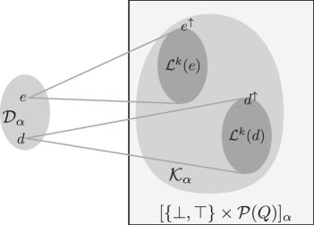
Figure 2. Model $\mathcal{D}$ is embeded into model $\mathcal{K}$ via logical relation $\mathcal{L}$.

Figure 2 shows the intuition behind the construction. Every $\mathcal{K}_{\alpha}$ is finite since it lives inside the standard model constructed from $\mathcal{D}_{0}\times\mathcal{P}(Q)$ as the base set. Moreover, as we shall see later, for every $\alpha$, $\mathcal{K}_{\alpha}$ is a join semilattice and thus has a greatest element. The logical relation $\mathcal{L}$ will divide $\mathcal{K}_{\alpha}$ into equivalence classes, one for every element of $\mathcal{D}_{\alpha}$. Every equivalence class will also have semilattice structure.

Recall that a TAC automaton is supposed to accept unsolvable terms from states $Q_{\Omega}$. So the unsolvable terms of type $0$ should have $Q_{\Omega}$ as a part of their meaning. This is why $\bot$ of $\mathcal{D}_{0}$ is associated to $(\bot,Q_{\Omega})$ in $\mathcal{K}_{0}$ via the relation $\mathcal{L}_{0}$. This also explains why we needed to take the least fixpoint in $\mathcal{D}$. If we had taken the greatest fixpoint then the unsolvable terms would have evaluated to $\top$ and the solvable ones to $\bot$. In consequence we would have needed to relate $\top$ with $(\top,Q_{\Omega})$, and we would have been forced to relate $\bot$ with $(\bot,Q)$. But then $(\top,Q_{\Omega})$ and $(\bot,Q)$ are incomparable in $\mathcal{K}_{0}$, and this makes it impossible to construct an order preserving injection from $\mathcal{D}_{0}$ to $\mathcal{K}_{0}$.

4.1.1. Structural properties of $\mathcal{K}(Q,Q_{\Omega})$

We are now going to present some properties of the partial orders $\mathcal{K}_{\alpha}$. The following lemma shows that for every type $\alpha$, $\mathcal{K}_{\alpha}$ is a join semilattice.

Lemma 7.

Given $(f_{1},d_{1})$ and $(f_{2},d_{2})$ in $\mathcal{L}_{\alpha}$, then $f_{1}\vee f_{2}$ is in $\mathcal{K}_{\alpha}$ and $(f_{1}\vee f_{2},d_{1}\vee d_{2})$ is in $\mathcal{L}_{\alpha}$.

Proof 4.1.

We proceed by induction on the structure of the type. For the base type the lemma is immediate from the definition. For the induction step consider a type of a form $\alpha\to\beta$ and assume that $f_{1}$ and $f_{2}$ in $\mathrm{mon}[\mathcal{K}_{\alpha}\to\mathcal{K}_{\beta}]$. Since, by induction, $\mathcal{K}_{\beta}$ is a join semilattice, we have that $f_{1}\vee f_{2}$ is also in $\mathrm{mon}[\mathcal{K}_{\alpha}\to\mathcal{K}_{\beta}]$. By the assumptions of the lemma, for every $(p,e)$ in $\mathcal{L}_{\alpha}$ we have $(f_{1}(p),d_{1}(e))$ and $(f_{2}(p),d_{2}(e))$ in $\mathcal{L}_{\beta}$. The induction hypothesis implies that $(f_{1}(p)\vee f_{2}(p),d_{1}(e)\vee d_{2}(e))$ is in $\mathcal{L}_{\beta}$. As by induction hypothesis $\mathcal{K}_{\beta}$ is a join semilattice, we get $(f_{1}\vee f_{2})(p)=f_{1}(p)\vee f_{2}(p)$ is in $\mathcal{K}_{\beta}$. Thus $((f_{1}\vee f_{2})(p),(d_{1}\vee d_{2})(e))$ is in $\mathcal{L}_{\beta}$. Since $(p,e)\in\mathcal{L}_{\alpha}$ was arbitrary this implies that $f_{1}\vee f_{2}$ is in $\mathcal{K}_{\alpha\to\beta}$ and $(f_{1}\vee f_{2},d_{1}\vee d_{2})$ is in $\mathcal{L}_{\alpha\to\beta}$.

A consequence of this lemma and of the finiteness of $\mathcal{K}_{\alpha}$ is that $\mathcal{K}_{\alpha}$ has a greatest element that we denote $\top\!\!\!\!\top_{\alpha}$. The lemma also implies the existence of certain meets.

Corollary 8.

For every type $\alpha$ and $f_{1},f_{2}$ in $\mathcal{K}_{\alpha}$. If there is $g\in\mathcal{K}_{\alpha}$ such that $g\leq f_{1}$ and $g\leq f_{2}$ then $f_{1}$ and $f_{2}$ have a greatest lower bound $f_{1}\land f_{2}$. Moreover, if $(f_{1},d_{1})$ and $(f_{2},d_{2})$ are in $\mathcal{L}_{\alpha}$ then $(f_{1}\land f_{2},d_{1}\land d_{2})$ is in $\mathcal{L}_{\alpha}$.

Proof 4.2.

Let $F=\{g\in\mathcal{K}_{\alpha}\mid g\leq f_{1}\text{ and }g\leq f_{2}\}$. As $\mathcal{K}_{\alpha}$ is finite, the set $F$ is finite. An iterative use of Lemma 7 shows that $\bigvee F$ exists and is in $\mathcal{K}_{\alpha}$. It is then straightforward to see that $\bigvee F$ is indeed the greatest lower bound of $f_{1}$ and $f_{2}$.

Now as $\mathcal{D}_{\alpha}$ is a complete lattice, we also have that $d_{1}\land d_{2}$ exits. Then a similar induction as in the proof of Lemma 7 shows that when $(f_{1},d_{1})$ and $(f_{2},d_{2})$ are in $\mathcal{L}_{\alpha}$, then $(f_{1}\land f_{2},d_{1}\land d_{2})$ is in $\mathcal{L}_{\alpha}$.

We are now going to show that every constant function of $\mathrm{mon}[\mathcal{K}_{\alpha}\to\mathcal{K}_{\beta}]$ is actually in $\mathcal{K}_{\alpha\to\beta}$.

Lemma 9.

For every $q$ in $\mathcal{K}_{\beta}$, the constant function $c_{q}\in\mathrm{mon}[\mathcal{K}_{\alpha}\to\mathcal{K}_{\beta}]$ assigning $q$ to every element of $\mathcal{K}_{\alpha}$ is in $\mathcal{K}_{\alpha\to\beta}$.

Proof 4.3.

To show that $c_{q}$ is in $\mathcal{K}_{\alpha\to\beta}$, we need to find $h_{q}$ in $\mathcal{D}_{\alpha\to\beta}$ such that for every $(p,e)$, $(c_{q}(p),h_{q}(e))$ is in $\mathcal{L}_{\beta}$. Since $q$ is in $\mathcal{K}_{\beta}$, there is $d$ such that $(q,d)$ is in $\mathcal{L}_{\beta}$. It suffices to take $h_{q}$ to be the function of $\mathcal{D}_{\alpha\to\beta}$ such that for every $e$ in $\mathcal{D}_{\alpha}$, $h_{q}(e)=d$.

As one easily observes that for every $p\in\mathcal{K}_{\alpha}$, $\top\!\!\!\!\top_{\alpha\to\beta}(p)=\top\!\!\!\!\top_{\beta}$, a consequence of this lemma is that $(\top\!\!\!\!\top_{\alpha},\top_{\alpha})$ is in $\mathcal{L}_{\alpha}$ for every $\alpha$.

This lemma allows us to define inductively on types the family of constant functions $(\bot\!\!\!\!\bot_{\alpha})_{\alpha\in\mathcal{T}}$ as follows:

1. $\bot\!\!\!\!\bot_{0}=(\bot,Q_{\Omega})$,

2. $\bot\!\!\!\!\bot_{\alpha\to\beta}(h)=\bot\!\!\!\!\bot_{\beta}$ for every $h$ in $\mathcal{K}_{\alpha}$.

Notice that $\bot\!\!\!\!\bot_{\alpha}$ is a minimal element of $\mathcal{K}_{\alpha}$, but $\mathcal{K}_{\alpha}$ does not have a least element in general.

4.1.2. Galois connections between $\mathcal{K}_{\alpha}$ and $\mathcal{D}_{\alpha}$

In this part, we wish to show that the relation $\mathcal{L}_{\alpha}$ is indeed defining an injection from $\mathcal{K}_{\alpha}$ to $\mathcal{D}_{\alpha}$ that we shall denote with $(\overline{\cdot})$. Moreover, we are going to define a mapping $(\cdot)^{\uparrow}$ from $\mathcal{D}_{\alpha}$ to $\mathcal{K}_{\alpha}$ so that $(\overline{\cdot})$ and $(\cdot)^{\uparrow}$ define a Galois connection between $\mathcal{K}_{\alpha}$ and $\mathcal{D}_{\alpha}$. This Galois connection plays a key role in allowing the model to track convergence and, thus, in the definition of the interpretation of fixpoints in the model. We shall also see that both $(\overline{\cdot})$ and $(\cdot)^{\uparrow}$ commute with application.

So as to define this Galois connection, we need to introduce the notion of $\mathcal{D}$-completeness of types. This notion imposes some basic properties that allow us to construct both $(\overline{\cdot})$ and $(\cdot)^{\uparrow}$. Our goal is to establish that every type is $\mathcal{D}$-complete.

For every $d$ in $\mathcal{D}_{\alpha}$, we denote by $L_{d}$ the set of elements of $\mathcal{K}_{\alpha}$ that are related to it:

$$L_{d}=\{p\in\mathcal{K}_{\alpha}\mid(p,d)\in\mathcal{L}_{\alpha}\}.$$

A type $\alpha$ is $\mathcal{D}$-complete if, for every $d$ in $\mathcal{D}_{\alpha}$:

1. $L_{d}$ is not empty,

2. $\bot\!\!\!\!\bot_{\alpha}\leq\bigvee L_{d}$,

3. for every $(f,e)$ in $\mathcal{L}_{\alpha}$: $f\leq\bigvee L_{d}$ iff $e\leq d$.

Later we will show that every type is $\mathcal{D}$-complete, but for this we will need some preparatory lemmas.

Lemma 10.

If $\alpha$ is a $\mathcal{D}$-complete type and $d$ is in $\mathcal{D}_{\alpha}$ then $(\bigvee L_{d},d)$ is in $\mathcal{L}_{\alpha}$.

Proof 4.4.

Since $\alpha$ is $\mathcal{D}$-complete, $L_{d}$ is not empty, and the conclusion follows directly from Lemma 7.

Lemma 11.

If $\alpha$ is a $\mathcal{D}$-complete type, and $d,e\in\mathcal{D}_{\alpha}$ then: $e\leq d$ iff $\bigvee L_{e}\leq\bigvee L_{d}$.

Proof 4.5.

As $\alpha$ is $\mathcal{D}$-complete both $L_{e}$ and $L_{d}$ are not empty and therefore, $\bigvee L_{e}$ and $\bigvee L_{d}$ are well-defined. Lemma 10 also gives that $(\bigvee L_{e},e)$ is in $\mathcal{L}_{\alpha}$. Now from $\mathcal{D}$-completeness of $\alpha$, we have that $\bigvee L_{e}\leq\bigvee L_{d}$ iff $e\leq d$.

The next step is to define the operation $(\cdot)^{\uparrow}$ that, as we will show later, is an embedding of $\mathcal{D}$ into $\mathcal{K}$. For this we need the notion of co-step functions that are particular functions from a partial order $L_{1}$ to a partial order $L_{2}$, the latter having the greatest element $\top_{2}$. Given two elements $p$ in $L_{1}$ and $q$ in $L_{2}$, the co-step function $p\nearrow q$ is a function from $\mathrm{mon}[L_{1}\to L_{2}]$ such that for $r$ in $L_{1}$,

$$(p\nearrow q)(r)=\begin{cases}q&\text{ when }r\leq p\\ \top_{2}&\text{otherwise}\ .\end{cases}$$

Let $\alpha,\beta$ be $\mathcal{D}$-complete types. For every $h\in\mathcal{D}_{\alpha\to\beta}$ and every $d\in\mathcal{D}_{\alpha}$ we define two monotone functions and the element $h^{\uparrow}$:

$$f_{h,d}=\bigvee L_{d}\nearrow\bigvee L_{h(d)},\qquad\overline{f}_{h,d}=d\nearrow h(d),$$

$$h^{\uparrow}=\bigwedge_{d\in\mathcal{D}}f_{h,d}\ .$$

For $h$ in $\mathcal{D}_{0}$, we define $h^{\uparrow}$ to be $(\bot,Q_{\Omega})$ when $h=\bot$, and to be $(\top,Q)$ when $h=\top$.

The next lemma summarizes all the essential properties of the model $\mathcal{K}$.

Lemma 12.

For all $\mathcal{D}$-complete types $\alpha$, $\beta$, for every $h\in\mathcal{D}_{\alpha\to\beta}$ and every $d\in\mathcal{D}_{\alpha}$:

1. $(f_{h,d},\overline{f}_{h,d})$ is in $\mathcal{L}_{\alpha\to\beta}$;

2. $\bot\!\!\!\!\bot_{\alpha\to\beta}\leq f_{h,d}$;

3. $h^{\uparrow}$ is an element of $\mathcal{K}_{\alpha\to\beta}$ and $(h^{\uparrow},h)\in\mathcal{L}_{\alpha\to\beta}$;

4. if $(p,e)\in\mathcal{L}_{\alpha}$ then $h^{\uparrow}(p)=\bigvee L_{h(e)}$;

5. $h^{\uparrow}=\bigvee L_{h}$.

Proof 4.6.

For the first item we take $(p,e)\in\mathcal{L}_{\alpha}$, and show that $(f_{h,d}(p),\overline{f}_{h,d}(e))\in\mathcal{L}_{\beta}$. This will be sufficient by the definition of $\mathcal{L}_{\alpha\to\beta}$. Lemma 10 gives $(\bigvee L_{d},d)\in\mathcal{L}_{\alpha}$ and $(\bigvee L_{h(d)},h(d))\in\mathcal{L}_{\beta}$. By $\mathcal{D}$-completeness of $\alpha$: $p\leq\bigvee L_{d}$ iff $e\leq d$. We have two cases. If $p\leq\bigvee L_{d}$ then $f_{h,d}(p)=\bigvee L_{h(d)}$ and $\overline{f}_{h,d}(e)=h(d)$. Otherwise, $p\nleq\bigvee L_{d}$ gives $f_{h,d}(p)=\top\!\!\!\!\top_{\beta}$ and $\overline{f}_{h,d}(e)=\top_{\beta}$. With the help of Lemma 10 in both cases we have that the result is in $\mathcal{L}_{\beta}$, and we are done.

For the second item, by $\mathcal{D}$-completeness of $\beta$ we have $\bigvee L_{h(d)}\geq\bot\!\!\!\!\bot_{\beta}$. In the proof of the first item we have seen that $f_{h,d}(p)\geq\bigvee L_{h(d)}$ for every $p\in\mathcal{K}_{\alpha}$. Since $\bot\!\!\!\!\bot_{\alpha\to\beta}(p)=\bot\!\!\!\!\bot_{\beta}$ we get $\bot\!\!\!\!\bot_{\alpha\to\beta}\leq f_{h,d}$.

In order to show the third item we use the first item telling us that $(f_{h,e},\overline{f}_{h,e})$ is in $\mathcal{L}_{\alpha\to\beta}$ for every $e\in\mathcal{D}_{\alpha}$. Since by the second item $\bot\!\!\!\!\bot_{\alpha}\leq f_{h,e}$, Corollary 8 shows that $(\bigwedge_{e\in\mathcal{D}_{\alpha}}f_{h,e},\bigwedge_{e\in\mathcal{D}_{\alpha}}\overline{f}_{h,e})$ is in $\mathcal{L}_{\alpha\to\beta}$. Directly from the definition of co-step functions we have $\bigwedge_{e\in\mathcal{D}_{\alpha}}e\nearrow h(e)=h$. This gives, as desired, $(\bigwedge_{e\in\mathcal{D}_{\alpha}}f_{h,e},h)$ in $\mathcal{L}_{\alpha\to\beta}$.

For the fourth item, take an arbitrary $(p,e)\in\mathcal{L}_{\alpha}$. We show that $h^{\uparrow}(p)=\bigvee L_{d(e)}$. By definition $h^{\uparrow}(p)=\bigwedge_{e^{\prime}\in\mathcal{D}_{\alpha}}f_{h,e^{\prime}}(p)$. Moreover $f_{h,e^{\prime}}(p)=\bigvee L_{h(e^{\prime})}$ if $p\leq\bigvee L_{e^{\prime}}$, and $f_{h,e^{\prime}}(p)=\top\!\!\!\!\top_{\beta}$ otherwise. By $\mathcal{D}$-completeness of $\alpha$: $p\leq\bigvee L_{e^{\prime}}$ iff $e\leq e^{\prime}$. So $h^{\uparrow}(p)=\bigwedge_{e^{\prime}\in\mathcal{D}_{\alpha}}f_{h,e^{\prime}}(p)=\bigwedge\{\bigvee L_{h(e^{\prime})}:e\leq e^{\prime}\}$. By Lemma 11, if $e\leq e^{\prime}$ then $\bigvee L_{h(e)}\leq\bigvee L_{h(e^{\prime})}$. Hence $h^{\uparrow}(p)=\bigvee L_{h(e)}$.

For the last item we want to show that $h^{\uparrow}=\bigvee L_{h}$. We know that $h^{\uparrow}\in L_{h}=\{g\in\mathcal{K}_{\alpha\to\beta}:(g,h)\in\mathcal{L}_{\alpha}\}$ since $(h^{\uparrow},h)\in\mathcal{L}_{\alpha\to\beta}$ by the third item. We show that for every $g\in L_{h}$, $g\leq h^{\uparrow}$. Take some $(p,e)\in\mathcal{L}_{\alpha}$. We have $(g(p),h(e))\in\mathcal{L}_{\beta}$, hence $g(p)\leq\bigvee L_{h(e)}$ by definition of $L_{h(e)}$. Since $h^{\uparrow}(p)=\bigvee L_{h(e)}$ by the fourth item, we get $g\leq h^{\uparrow}$.

Lemma 13.

Every type $\alpha$ is $\mathcal{D}$-complete.

Proof 4.7.

This is proved by induction on the structure of the type. The case of the base type follows by direct examination. For the induction step consider a type $\alpha\to\beta$ and suppose that $\alpha$ and $\beta$ are $\mathcal{D}$-complete. Given $d$ in $\mathcal{D}_{\alpha\to\beta}$, Lemma 12 gives that $(d^{\uparrow},d)$ is in $\mathcal{L}_{\alpha\to\beta}$ proving that $L_{d}\neq\emptyset$, it also gives that $\bot\!\!\!\!\bot_{\alpha\to\beta}\leq d^{\uparrow}$ and $d^{\uparrow}=\bigvee L_{d}$, so we obtain $\bot\!\!\!\!\bot_{\alpha\to\beta}\leq\bigvee L_{d}$. It just remains to prove that for every $(f,e)$ in $\mathcal{L}_{\alpha\to\beta}$: $f\leq\bigvee L_{d}$ iff $e\leq d$.

We first remark that, as by induction hypothesis, $\alpha$ and $\beta$ are $\mathcal{D}$-complete, by Lemma 12 (items (4) and (5)), for every $(p,e^{\prime})\in\mathcal{L}_{\alpha}$ we have:

$$\bigvee L_{d(e^{\prime})}=d^{\uparrow}(p)=\left(\bigvee L_{d}\right)(p)$$ (1)

Let’s first suppose that $e\leq d$. Take a $p\in\mathcal{K}_{\alpha}$. By definition of the model there is $e^{\prime}$, such that $(p,e^{\prime})\in\mathcal{L}_{\alpha}$. As $\alpha$ is $\mathcal{D}$-complete, Lemma 11 gives us $\bigvee L_{e(e^{\prime})}\leq\bigvee L_{d(e^{\prime})}$. By definition of $\mathcal{L}_{\alpha\to\beta}$ we have that $(f(p),e(e^{\prime}))\in\mathcal{L}_{\beta}$, so $f(p)\leq\bigvee L_{e(e^{\prime})}$ by definition of $L_{e(e^{\prime})}$. This gives $f(p)\leq\bigvee L_{e(e^{\prime})}\leq\bigvee L_{d(e^{\prime})}$. Finally Equation (1) shows the desired $f(p)\leq\left(\bigvee L_{d}\right)(p)$ for every $p\in\mathcal{K}_{\alpha}$.

Let us now suppose that $f\leq\bigvee L_{d}$. The $\mathcal{D}$-completeness of $\alpha$ tells us that for every $e^{\prime}$ in $\mathcal{D}_{\alpha}$ there is $p$ in $\mathcal{K}_{\alpha}$ so that $(p,e^{\prime})$ is in $\mathcal{L}_{\alpha}$. Then Equation (1) gives $f(p)\leq\left(\bigvee L_{d}\right)(p)=\bigvee L_{d(e^{\prime})}$. Now, as by induction $\beta$ is $\mathcal{D}$-complete, the fact that $(f(p),e(e^{\prime}))\in\mathcal{L}_{\beta}$ entails $e(e^{\prime})\leq d(e^{\prime})$. As $e^{\prime}$ was arbitrary we obtain $e\leq d$.

The proposition below sums up the properties of the embedding $(\cdot)^{\uparrow}$ from Definition 4.1.2.

Proposition 14.

Given a type $\alpha$, and $d$ in $\mathcal{D}_{\alpha}$, the element $d^{\uparrow}$ from $\mathcal{K}_{\alpha}$ is such that:

1. $(d^{\uparrow},d)$ is in $\mathcal{L}_{\alpha}$,

2. if $e\in\mathcal{D}_{\alpha}$ and $d\leq e$ then $d^{\uparrow}\leq e^{\uparrow}$,

3. if $(f,d)$ is in $\mathcal{L}_{\alpha}$, then $f\leq d^{\uparrow}$,

4. if $\alpha=\alpha_{1}\to\alpha_{2}$ and $(g,e)$ is in $\mathcal{L}_{\alpha_{1}}$ then $d^{\uparrow}(g)=(d(e))^{\uparrow}$

Proof 4.8.

These properties follow directly from Lemma 12, except for the second property for which a small calculation is needed. Since $(d^{\uparrow},d)$ is in $\mathcal{L}_{\alpha}$ and $d\leq e$ then by Lemma 12: $d^{\uparrow}\leq\bigvee L_{e}$. The latter is precisely $e^{\uparrow}$ by Lemma 12.

In particular, in combination with item 3 of Lemma 12 , this proposition shows that the operator $(\cdot)^{\uparrow}$ commutes with the application: $d^{\uparrow}(e^{\uparrow})=(d(e))^{\uparrow}$.

The next lemma shows that the relation $\mathcal{L}_{\alpha}$ is functional.

Lemma 15.

For every type $\alpha$ and $f$ in $\mathcal{K}_{\alpha}$: if $(f,d_{1})$ and $(f,d_{2})$ are in $\mathcal{L}_{\alpha}$, then $d_{1}=d_{2}$.

Proof 4.9.

We proceed by induction on the structure of the type. The case of the base type follows from a direct inspection. For the induction step suppose that both $(f,d_{1})$ and $(f,d_{2})$ are in $\mathcal{L}_{\alpha\to\beta}$. Take an arbitrary $e\in\mathcal{D}_{\alpha}$. By Lemma 12 we have $(e^{\uparrow},e)\in\mathcal{L}_{\alpha}$. Therefore $(f(e^{\uparrow}),d_{1}(e))$ and $(f(e^{\uparrow}),d_{2}(e))$ in $\mathcal{L}_{\beta}$. The induction hypothesis implies that $d_{1}(e)=d_{2}(e)$. Since $e$ was arbitrary we get $d_{1}=d_{2}$.

Since, by definition, for every $f\in\mathcal{K}_{\alpha}$ we have $(f,d)\in\mathcal{L}_{\alpha}$ for some $d\in\mathcal{D}_{\alpha}$, the above lemma gives us a projection of $\mathcal{K}_{\alpha}$ to $\mathcal{D}_{\alpha}$. For this we re-use the notation we have introduced in Definition 4.1.2. For every type $\alpha$ and $f\in\mathcal{K}_{\alpha}$ we let $\overline{f}$ be the unique element of $\mathcal{D}_{\alpha}$ such that $(f,\overline{f})\in\mathcal{L}_{\alpha}$. Notice that $\overline{d^{\uparrow}}=d$ for every $d$ in $\mathcal{D}_{\alpha}$, since $(d^{\uparrow},d)$ is in $\mathcal{L}_{\alpha}$ by Proposition 14.

We immediately state some properties of the projection. We start by showing that it commutes with the application.

Lemma 16.

Given $f$ in $\mathcal{K}_{\alpha\to\beta}$ and $p$ in $\mathcal{K}_{\alpha}$, $\overline{f(p)}=\overline{f}(\overline{p})$.

Proof 4.10.

We have $(f,\overline{f})$ in $\mathcal{L}_{\alpha\to\beta}$ and $(p,\overline{p})$ in $\mathcal{L}_{\alpha}$, so that $(f(p),\overline{f}(\overline{p}))$ is in $\mathcal{L}_{\beta}$ and thus $\overline{f(p)}=\overline{f}(\overline{p})$.

Lemma 17.

Given $f$ and $g$ in $\mathcal{K}_{\alpha}$, if $f\leq g$ then $\overline{f}\leq\overline{g}$.

Proof 4.11.

We proceed by induction on the structure of the types. The case of the base type follows by a straightforward inspection. For the induction step take $f\leq g$ in $\mathcal{K}_{\alpha\to\beta}$. For an arbitrary $d\in\mathcal{D}_{\alpha}$ we have $f(d^{\uparrow})\leq g(d^{\uparrow})$. By induction hypothesis on type $\beta$ we get $\overline{f(d^{\uparrow})}\leq\overline{g(d^{\uparrow})}$. By Lemma 16 we obtain $\overline{f(d^{\uparrow})}=\overline{f}(\overline{d^{\uparrow}})=\overline{f}(d)$. The last equality follows from the fact that $\overline{d^{\uparrow}}=d$ since $(d^{\uparrow},d)$ is in $\mathcal{L}_{\alpha}$ by Proposition 14. Of course the same equalities hold for $g$ too. So $\overline{f}(d)\leq\overline{g}(d)$ for arbitrary $d$, and we are done.

Taking an abstract view on the operations $(\cdot)^{\uparrow}$ and $\overline{(\cdot)}$, we can summarise all the properties we have shown as follows:

Corollary 18.

For the models $\mathcal{D}$ and $\mathcal{K}$ as defined above.

1. Mapping $(\cdot)^{\uparrow}$ is a functor from $\mathcal{D}$ to $\mathcal{K}$.

2. Mapping $\overline{(\cdot)}$ is a functor from $\mathcal{K}$ to $\mathcal{D}$.

3. At every type both mappings are monotonous and moreover they form a Galois connection in the sense that $\overline{f}\leq d$ iff $f\leq d^{\uparrow}$.

4. The pair $\overline{(\cdot)}$, $(\cdot)^{\uparrow}$ forms a retraction: $\overline{d^{\uparrow}}=d$.

4.1.3. Interpretation of fixpoints

We are now going to give the definition of the interpretation of the fixpoint combinator in $\mathcal{K}$. This definition is based on that of the fixpoint operator in $\mathcal{D}$. We write $\mathrm{fix}_{\alpha}$ for the operation in $\mathcal{D}_{(\alpha\to\alpha)\to\alpha}$ that maps a function of $\mathcal{D}_{\alpha\to\alpha}$ to its least fixpoint.

Lemma 19.

Given $f$ in $\mathcal{K}_{\alpha\to\alpha}$, we have $f(\mathrm{fix}_{\alpha}(\overline{f})^{\uparrow})\leq\mathrm{fix}_{\alpha}(\overline{f})^{\uparrow}$.

Proof 4.12.

By proposition 14, $(\mathrm{fix}_{\alpha}(\overline{f})^{\uparrow},\mathrm{fix}_{\alpha}(\overline{f}))$ is in $\mathcal{L}_{\alpha}$. Moreover, as $(f,\overline{f})$ is in $\mathcal{L}_{\alpha\to\alpha}$, by definition of $\mathcal{L}_{\alpha\to\alpha}$, we have $(f(\mathrm{fix}_{\alpha}(\overline{f})^{\uparrow}),\overline{f}(\mathrm{fix}_{\alpha}(\overline{f})))=(f(\mathrm{fix}_{\alpha}(\overline{f})^{\uparrow}),\mathrm{fix}_{\alpha}(\overline{f}))$ is in $\mathcal{L}_{\alpha}$. Then by Proposition 14 we get $f(\mathrm{fix}_{\alpha}(\overline{f})^{\uparrow})\leq\mathrm{fix}_{\alpha}(\overline{f})^{\uparrow}$.

The above lemma guarantees that the sequence $f^{n}(\mathrm{fix}_{\alpha}(\overline{f})^{\uparrow})$ is decreasing. We can now define an operator that, as we will show, is the fixpoint operator we are looking for. For every type $\alpha$ and $f\in\mathcal{K}_{\alpha}$ define

$$\mathrm{Fix}_{\alpha}(f)=\bigwedge_{n\in\mathbb{N}}(f^{n}(\mathrm{fix}_{\alpha}(\overline{f})^{\uparrow}))\ .$$

We show that $\mathrm{Fix}_{\alpha}$ is monotone.

Lemma 20.

Given $f$ and $g$ in $\mathcal{K}_{\alpha\to\alpha}$, if $f\leq g$ then $\mathrm{Fix}_{\alpha}(f)\leq\mathrm{Fix}_{\alpha}(g)$.

Proof 4.13.

By Lemma 17, $f\leq g$ implies $\overline{f}\leq\overline{g}$, as $\mathrm{fix}_{\alpha}$ is monotone, we have $\mathrm{fix}_{\alpha}(\overline{f})\leq\mathrm{fix}_{\alpha}(\overline{g})$ and $\mathrm{fix}_{\alpha}(\overline{f})^{\uparrow}\leq\mathrm{fix}_{\alpha}(\overline{g})^{\uparrow}$ by Proposition 14. As $f\leq g$ we have $f^{k}(\mathrm{fix}_{\alpha}(\overline{f})^{\uparrow})\leq g^{k}(\mathrm{fix}_{\alpha}(\overline{g})^{\uparrow})$ for every $k$ in $\mathbb{N}$. Therefore $\bigwedge_{n\in\mathbb{N}}f^{n}(\mathrm{fix}_{\alpha}(\overline{f})^{\uparrow})\leq\bigwedge_{n\in\mathbb{N}}g^{n}(\mathrm{fix}_{\alpha}(\overline{g})^{\uparrow})$.

The last step is to show that $\mathrm{Fix}_{\alpha}$ is actually in $\mathcal{K}_{(\alpha\to\alpha)\to\alpha}$.

Lemma 21.

For every $\alpha$, $\mathrm{Fix}_{\alpha}$ is in $\mathcal{K}_{\alpha}$ and $(\mathrm{Fix}_{\alpha},\mathrm{fix}_{\alpha})$ is in $\mathcal{L}_{(\alpha\to\alpha)\to\alpha}$.

Proof 4.14.

We know that $(f,\overline{f})$ in $\mathcal{L}_{\alpha\to\alpha}$. As we have seen in the proof of Lemma 19, $(f(\mathrm{fix}_{\alpha}(\overline{f})^{\uparrow}),\mathrm{fix}_{\alpha}(\overline{f}))$ is in $\mathcal{L}_{\alpha}$. Using repeatedly the defining properties of $\mathcal{L}_{\alpha\to\alpha}$, we obtain that for every $n\in\mathbb{N}$, $(f^{n}(\mathrm{fix}_{\alpha}(\overline{f})^{\uparrow}),\mathrm{fix}_{\alpha}(\overline{f}))$ is in $\mathcal{L}_{\alpha}$. But $f^{n}(\mathrm{fix}_{\alpha}(\overline{f})^{\uparrow})$ is decreasing by Lemma 19. Since $\mathcal{K}_{\alpha}$ is finite, we get $(\bigwedge_{n\in\mathbb{N}}f^{n}(\mathrm{fix}_{\alpha}(\overline{f})^{\uparrow}),\mathrm{fix}_{\alpha}(\overline{f}))$ in $\mathcal{L}_{\alpha}$. We are done since $\bigwedge_{n\in\mathbb{N}}f^{n}(\mathrm{fix}_{\alpha}(\overline{f})^{\uparrow})=\mathrm{Fix}_{\alpha}(f)$.

4.1.4. A model of the $\lambda Y$-calculus

We are ready to define the model we were looking for.

For a finite set $Q$ and its subset $Q_{\Omega}\subseteq Q$ consider a tuple $\mathcal{K}(Q,Q_{\Omega},\rho)=(\{\mathcal{K}_{\alpha}\}_{\alpha\in\mathcal{T}},\rho)$ where $\{\mathcal{K}_{\alpha}\}_{\alpha\in\mathcal{T}}$ is as in Definition 4.1 and $\rho$ is a valuation such that for every type $\alpha$: $\omega^{\alpha}$ is interpreted as the greatest element of $\mathcal{K}_{\alpha}$, $Y^{(\alpha\to\alpha)\to\alpha}$ is interpreted as $\mathrm{Fix}_{\alpha}$, and $\Omega^{\alpha}$ is interpreted as $\bot\!\!\!\!\bot_{\alpha}$. Notice that, according to this definition, $\Omega^{0}$ is interpreted as $(\bot,Q_{\Omega})$. So the semantics of $\Omega$ and $\omega$ are different in this model. Recall that $\Omega$ is used to denote divergence, and $\omega$ is used in the definition of the truncation operation from the semantics of Böhm trees (cf. page 2.1).

We will show $\mathcal{K}(Q,Q_{\Omega},\rho)$ is indeed a model of the $\lambda Y$-calculus. Since $\mathcal{K}_{\alpha\to\beta}$ does not contain all the functions from $\mathcal{K}_{\alpha}$ to $\mathcal{K}_{\beta}$ we must show that there are enough of them to form a model of $\lambda Y$, the main problem being to show that ${[\![\lambda x.M]\!]}^{\upsilon}_{\mathcal{K}}$ defines an element of $\mathcal{K}$. For this, it is sufficient to prove that constant functions and the combinators $S$ and $K$ exist in the model.

Lemma 22.

For every sequence of types $\vec{\alpha}=\alpha_{1}\ldots\alpha_{n}$ and every types $\beta$, $\gamma$ we have the following:

• For every constant $p\in\mathcal{K}_{\beta}$ the constant function $f_{p}:\alpha_{1}\to\dots\to\alpha_{n}\to\beta$ belongs to $\mathcal{K}$.

• For $i=1,\dots,n$, the projection $\pi_{i}:\alpha_{1}\to\dots\to\alpha_{n}\to\alpha_{i}$ belongs to $\mathcal{K}$.

• If $f:\vec{\alpha}\to(\beta\to\gamma)$ and $g:\vec{\alpha}\to\beta$ are in $\mathcal{K}$ then $\lambda\vec{p}.f\vec{p}(g\vec{p}):\vec{\alpha}\to\gamma$ is in $\mathcal{K}$.

Proof 4.15.

The first item of the lemma is given by Lemma 9, the second does not present more difficulty. Finally, the third proceeds by a direct examination once we observe the following property of $\mathcal{K}(Q,Q_{\Omega},\rho)$. Given two elements $f$ of $\mathrm{mon}[\mathcal{K}_{\alpha_{1}}\to\cdots\to\mathrm{mon}[\mathcal{K}_{\alpha_{n}}\to\mathcal{K}_{\beta}]]$ and $g$ of $\mathcal{D}_{\alpha_{1}\to\cdots\to\alpha_{n}\to\beta}$, if for every $d_{1}$, …, $d_{n}$ in $\mathcal{K}_{\alpha_{1}}$, …, $\mathcal{K}_{\alpha_{n}}$, $(f(d_{1},\ldots,d_{n}),g(\overline{d_{1}},\ldots,\overline{d_{n}}))\in\mathcal{L}_{\beta}$ then $f$ is in $\mathcal{K}_{\alpha_{1}\to\cdots\to\alpha_{n}\to\beta}$ and $(f,g)$ is in $\mathcal{L}_{\alpha_{1}\to\cdots\to\alpha_{n}\to\beta}$. This observation follows directly from Proposition 14 and the definition of the model.

The above lemma allows us to define the interpretation of terms in the usual way:

• ${[\![Y^{(\beta\to\beta)\to\beta}]\!]}^{\upsilon}_{\mathcal{K}}=\mathrm{Fix}_{\beta}$

• ${[\![a]\!]}_{\mathcal{K}}^{\upsilon}=\rho(a)$

• ${[\![x^{\alpha}]\!]}^{\upsilon}_{\mathcal{K}}=\upsilon(x)$

• ${[\![\omega^{\beta}]\!]}_{\mathcal{K}}^{\upsilon}=\top\!\!\!\!\top_{\beta}$

• ${[\![\Omega^{\beta}]\!]}_{\mathcal{K}}^{\upsilon}=\bot\!\!\!\!\bot_{\beta}$

• ${[\![MN]\!]}_{\mathcal{K}}^{\upsilon}={[\![M]\!]}_{\mathcal{K}}^{\upsilon}({[\![N]\!]}^{\upsilon}_{\mathcal{K}})$

• ${[\![\lambda x^{\alpha}.M]\!]}_{\mathcal{K}}^{\upsilon}(a)={[\![M]\!]}_{\mathcal{K}}^{[\upsilon[a/x]]}$, for every $a\in\mathcal{K}_{\alpha}$.

We need to check that for every valuation $\upsilon$ and every term $M$ of type $\alpha$, ${[\![M]\!]}^{\upsilon}_{\mathcal{K}}$ is indeed in $\mathcal{K}_{\alpha}$. For this we take a list of variables $x_{1}^{\alpha_{1}}$, …, $x_{n}^{\alpha_{n}}$ containing all free varaibles of $M$, and we show that the function $\lambda p_{1}\dots p_{n}.{[\![M]\!]}^{[p_{1}/x_{1},\dots,p_{n}/x_{n}]}_{\mathcal{K}}$ is in $\mathcal{K}_{\alpha_{1}\to\cdots\to\alpha_{n}\to\alpha}$. The proof is a simple induction on the structure of $M$. Lemma 21 and Lemma 22 ensure that this is the case when $M=Y$. For the other constants, $a$, $\omega$ and $\Omega$, we use the fact that constant functions are in the model. The remaining cases are handled by Lemma 22: variable and application clauses use $K$ and $S$ combinators respectively.

These observations allow us to conclude that $\mathcal{K}(Q,Q_{\Omega},\rho)$ is indeed a model of the $\lambda Y$-calculus, that is:

1. for every term $M$ of type $\alpha$ and every valuation $\upsilon$ ranging of the free variables of $M$, ${[\![M]\!]}^{\upsilon}_{\mathcal{K}}$ is in $\mathcal{K}_{\alpha}$,

2. given two terms $M$ and $N$ of type $\alpha$, if $M=_{\beta\delta}N$, then for every valuation $\upsilon$, ${[\![M]\!]}^{\upsilon}_{\mathcal{K}}={[\![N]\!]}^{\upsilon}_{\mathcal{K}}$.

Theorem 23.

For every finite set $Q$ and every set $Q_{\Omega}\subseteq Q$ the model $\mathcal{K}(Q,Q_{\Omega},\rho)$ as in Definition 4.1.4 is a model of the $\lambda Y$-calculus.

Let us mention the following useful fact showing a correspondence between the meanings of a term in $\mathcal{K}$ and in $\mathcal{D}$. The proof is immediate since $\{\mathcal{L}_{\alpha}\}_{\alpha\in\mathcal{T}}$ is a logical relation (cf [AC98]).

Lemma 24.

For every type $\alpha$ and closed term $M$ of type $\alpha$:

$$({[\![M]\!]}_{\mathcal{K}},{[\![M]\!]}_{\mathcal{D}})\in\mathcal{L}_{\alpha}\,.$$

4.2. Correctness and completeness of the model

It remains to show that the model we have constructed is indeed sufficient to recognize languages of TAC automata. For the rest of the section we fix a tree signature $\Sigma$ and a TAC automaton

$$\mathcal{A}=\langle Q,\Sigma,q^{0}\in Q,\delta_{1}:Q\times\Sigma_{1}\to\{\mathit{ff},\mathit{tt}\},\delta_{2}:Q\times\Sigma_{2}\to\mathcal{P}(Q^{2})\rangle\ .$$

We take a model $\mathcal{K}$ based on $\mathcal{K}(Q,Q_{\Omega},\rho)$ as in Definition 4.1.4, where $Q_{\Omega}$ is the set of states $q$ such that $\delta(q,\Omega)=\mathit{tt}$. It remains to specify the meaning of constants like $c:0$ or $a:0^{2}\to 0$ in $\Sigma$:

$$\rho(c)= (\top,\{q:\delta(q,c)=\mathit{tt}\})$$

$$\rho(a)(d_{1},R_{1})(d_{2},R_{2})= (\top,R)\qquad\text{where $d_{1},d_{2}\in\{\bot,\top\}$ and }$$

$$\quad R=\{q\in Q\mid\delta(q,a)\cap R_{1}\times R_{2}\not=\emptyset\}\ .$$

Lemma 25.

For every $a$ in $\Sigma$ of type $o^{2}\to o$: $\rho(a)$ is in $\mathcal{K}_{o^{2}\to o}$ and $(\rho(a),\top_{o^{2}\to o})$ is in $\mathcal{L}_{o^{2}\to o}$.

Proof 4.16.

It is easy to see that $\rho(a)$ is monotone. For the membership in $\mathcal{K}$ the witnessing function from $\mathcal{D}_{o^{2}\to o}$ is $\top_{0^{2}\to 0}$.

Once we know that $\mathcal{K}$ is a model we can state some of its useful properties. The first one tells what the meaning of unsolvable terms is. The second indicates how unsolvability is taken into account in the computation of a fixpoint.

Proposition 26.

Given a closed term $M$ of type $0$: $BT(M)=\Omega^{0}$ iff ${[\![M]\!]}_{\mathcal{K}}=(\bot,Q_{\Omega})$.

Proof 4.17.

If ${[\![M]\!]}_{\mathcal{K}}=(\bot,Q_{\Omega})$ then Lemma 24 gives us ${[\![M]\!]}_{\mathcal{D}}=\bot$. By Theorem 6 this implies $BT(M)=\Omega^{0}$.

If $BT(M)=\Omega^{0}$ then Theorem 6 entails that ${[\![M]\!]}_{\mathcal{D}}=\bot$. By Lemma 24 $({[\![M]\!]}_{\mathcal{K}},\bot)$ is in $\mathcal{L}_{0}$. But this is possible only if ${[\![M]\!]}_{\mathcal{K}}=(\bot,Q_{\Omega})$.

Lemma 27.

Given a type $\beta=\beta_{1}\to\dots\to\beta_{l}\to 0$, a sequence of types $\vec{\alpha}=\alpha_{1},\dots,\alpha_{k}$, and a function $f\in\mathcal{K}_{\vec{\alpha}\to\beta\to\beta}$, consider the functions:

$$h=\lambda p_{1}\dots p_{k}.\left(\mathrm{fix}_{\beta}(\overline{f(p_{1})\dots(p_{k})})\right)^{\uparrow}\qquad g=\lambda e_{1}\dots e_{k}.\mathrm{fix}_{\beta}(\overline{f}(e_{1})\dots(e_{k}))$$

that are respectively in $\mathrm{mon}[\mathcal{K}_{\alpha_{1}}\to\dots\to\mathrm{mon}[\mathcal{K}_{\alpha_{k}}\to\mathcal{K}_{\beta}]]$ and in $\mathcal{D}_{\vec{\alpha}\to\beta}$. Then $h$ is in $\mathcal{K}_{\vec{\alpha}\to\beta}$ and $(h,g)$ is in $\mathcal{L}_{\vec{\alpha}\to\beta}$. Moreover, for every $p_{1}\in\mathcal{K}_{\alpha_{1}}$, …, $p_{k}\in\mathcal{K}_{\alpha_{k}}$, $q_{1}\in\mathcal{K}_{\beta_{1}}$,…, $q_{l}\in\mathcal{K}_{\beta_{l}}$ we have

$$h(p_{1},\dots,p_{k})(q_{1},\dots,p_{l})=\begin{cases}(\bot,Q_{\Omega})&\text{if $g(\overline{p}_{1},\dots,\overline{p}_{k})(\overline{q}_{1},\dots,\overline{q}_{l})=\bot$}\\ (\top,Q)&\text{if $g(\overline{p}_{1},\dots,\overline{p}_{k})(\overline{q}_{1},\dots,\overline{q}_{l})=\top$}\ .\end{cases}$$

Proof 4.18.

To prove that $(h,g)$ is in $\mathcal{L}_{\vec{\alpha}\to\beta}$, we resort to the remark we made in the proof of Lemma 22, so that it suffices to show that for every $p_{1}$, …, $p_{k}$ respectively in $\mathcal{K}_{\alpha_{1}}$, …, $\mathcal{K}_{\alpha_{k}}$, $(h(p_{1},\ldots,p_{k}),g(\overline{p}_{1},\dots,\overline{p}_{k}))$ is in $\mathcal{L}_{\beta}$. We have that $h(p_{1},\dots,p_{k})=\left(\mathrm{fix}_{\beta}(\overline{f(p_{1},\dots,p_{k})})\right)^{\uparrow}$ that is in $\mathcal{K}_{\beta}$, and then

$$\overline{h(p_{1},\dots,p_{k})} = \overline{\left(\mathrm{fix}_{\alpha}(\overline{f(p_{1},\dots,p_{k})})\right)^{\uparrow}}$$

$$= \mathrm{fix}_{\alpha}(\overline{f(p_{1},\dots,p_{k})})$$

$$= \mathrm{fix}_{\alpha}(\overline{f}(\overline{p}_{1},\dots,\overline{p}_{k}))\text{ by successive use of Lemma~{}\ref{lem:commutation_overline_application}}$$

$$= g(\overline{p_{1}},\dots,\overline{p}_{k})\ .$$

This shows that $(h,g)$ is in $\mathcal{L}_{\vec{\alpha}\to\beta}$ and thus $h$ is in $\mathcal{K}_{\vec{\alpha}\to\beta}$.

So as to complete the proof of the lemma, we first prove the following claim: for every for $r$ in $\mathcal{D}_{\gamma_{1}\to\dots\to\gamma_{n}\to 0}$, and $q_{1}$, …, $q_{n}$ in $\mathcal{K}_{\gamma_{1}}$, …, $\mathcal{K}_{\gamma_{n}}$ we have that:

• $r^{\uparrow}(q_{1},\dots,q_{n})=(\bot,Q_{\Omega})$ iff $(r(\overline{q_{1}},\dots,\overline{q_{n}}))^{\uparrow}=(\bot,Q_{\Omega})$,

• $r^{\uparrow}(q_{1},\dots,q_{n})=(\top,Q)$ iff $(r(\overline{q_{1}},\dots,\overline{q_{n}}))^{\uparrow}=(\top,Q)$.

We first remark that, given $r$ in $\mathcal{D}_{\gamma\to\delta}$, from the fourth item of Proposition 14, we have that whenever $(q,e)$ is in $\mathcal{L}_{\gamma}$, then $r^{\uparrow}(q)=(r(e))^{\uparrow}$, so that in particular $r^{\uparrow}(q)=(r(\overline{q}))^{\uparrow}$. A simple induction shows then that, for $r$ in $\mathcal{D}_{\gamma_{1}\to\dots\to\gamma_{n}\to\delta}$,

$$r^{\uparrow}(q_{1},\dots,q_{n})=(r(\overline{q_{1}},\dots,\overline{q_{n}}))^{\uparrow}\ .$$

Therefore if $\delta=0$ and $r(\overline{q_{1}},\dots,\overline{q_{n}})=\bot$, we have $(r(\overline{q_{1}},\dots,\overline{q_{n}}))^{\uparrow}=(\bot,Q_{\Omega})$. Moreover, in case $r(\overline{q_{1}},\dots,\overline{q_{n}})=\top$, we have $(r(\overline{q_{1}},\dots,\overline{q_{n}}))^{\uparrow}=(\top,Q)$.

Now, the lemma follows from choosing $r=g(\overline{p}_{1},\dots,\overline{p}_{k})$ and remarking that we have $(g(\overline{p}_{1},\dots,\overline{p}_{k}))^{\uparrow}=h(p_{1},\ldots,p_{k})$.

As in the case of GFP-models the semantics of a Böhm tree is defined in terms of its truncations: ${[\![BT(M)]\!]}_{\mathcal{K}}=\bigwedge\{{[\![BT(M)\!\downarrow_{n}]\!]}_{\mathcal{K}}\mid n\in\mathbb{N}\}$. The subtle difference is that now $\Omega^{0}$ and $\omega^{0}$ do not have the same meaning. Nevertheless, the analog of Proposition 2 still holds in $\mathcal{K}$.

Theorem 28.

For very closed term $M$ of type $0$: ${[\![M]\!]}_{\mathcal{K}}={[\![BT(M)]\!]}_{\mathcal{K}}$.

Proof 4.19.

First we show that ${[\![M]\!]}_{\mathcal{K}}\leq{[\![BT(M)]\!]}_{\mathcal{K}}$. For this, we proceed with the classical finite approximation technique. We thus define a finite approximation of the Böhm tree. The Abstract Böhm tree up to depth $l$ of a term $M$, denoted $ABT_{l}(M)$, will be a term obtained by reducing $M$ till it resembles $BT(M)$ up to depth $l$ as much as possible. We define it by induction:

• $ABT_{0}(M)=M$;

• $ABT_{l+1}(M)$ is $M$ if $M$ does not have head normal form,
  otherwise it is a term $\lambda\vec{x}.N_{0}ABT_{l}(N_{1})\dots ABT_{l}(N_{k})$, where $\lambda\vec{x}.N_{0}N_{1}\dots N_{k}$ is the head normal form of $M$.

Since $ABT_{l}(M)$ is obtained from $M$ by a sequence of $\beta\delta$-reductions, ${[\![M]\!]}_{\mathcal{K}}={[\![ABT_{l}(M)]\!]}_{\mathcal{K}}$ for every $l$. We now show that for every term $M$ and every $l$:

$${[\![ABT_{l}(M)]\!]}_{\mathcal{K}}\leq{[\![BT(M)\!\downarrow_{l}]\!]}_{\mathcal{K}}.$$

Up to depth $l$, the two terms have the same structure as trees. We will see that the meaning of every leaf in $ABT_{l}(M)$ is not bigger than the meaning of the corresponding leaf of $BT(M)\!\downarrow_{l}$. For leaves of depth $l$ this is trivial since on the one hand we have a term and on the other the constant $\omega$. For other leaves, the terms are either identical and thus have the same interpretation or on one side we have a term without head normal form and on the other $\Omega^{0}$ and thus, according to Proposition 26 also have the same interpretation.

The desired inequality ${[\![M]\!]}_{\mathcal{K}}\leq{[\![BT(M)]\!]}_{\mathcal{K}}$ follows now directly from the definition of the semantics of $BT(M)$ since ${[\![M]\!]}_{\mathcal{K}}={[\![ABT_{l}(M)]\!]}_{\mathcal{K}}\leq{[\![BT(M)\!\downarrow_{l}]\!]}_{\mathcal{K}}$ for every $l\in\mathbb{N}$; and ${[\![BT(M)]\!]}_{\mathcal{K}}=\bigwedge\{{[\![BT(M)\!\downarrow_{l}]\!]}_{\mathcal{K}}\mid l\in\mathbb{N}\}$.

For the inequality in the other direction, we also use a classical method that consists of working with finite unfoldings of the $Y$ combinators. Observe that if a term $M$ does not have $Y$ combinators, then it is strongly normalizing and the theorem is trivial. So we need be able to deal with $Y$ combinators in $M$. For this we introduce new constants $c_{N}$ for every subterm $YN$ of $M$. The type of $c_{N}$ is $\vec{\alpha}\to\beta$ if $\beta$ is the type of $YN$ and $\vec{\alpha}=\alpha_{1}\dots\alpha_{k}$ is the sequence of types of the sequence of free variables $\vec{x}=x_{1}\dots x_{k}$ occurring in $YN$. We let the semantics of a constant $c_{N}$ be

$${[\![c_{N}]\!]}_{\mathcal{K}}=\lambda\vec{p}.\left(\mathrm{fix}_{\beta}(\overline{{[\![N]\!]}_{\mathcal{D}}^{[\vec{p}/\vec{x}]}})\right)^{\uparrow}\ .$$

First we need to check that indeed ${[\![c_{N}]\!]}_{\mathcal{K}}$ is in $\mathcal{K}$. For this we have prepared Lemma 27. Indeed ${[\![c_{N}]\!]}_{\mathcal{K}}=\lambda p_{1}\dots p_{k}.\ \left(\mathrm{fix}_{\beta}(\overline{f(p_{1},\dots,p_{k})})\right)^{\uparrow}$, for $f=\lambda\vec{p}.\ {[\![N]\!]}^{[\vec{p}/\vec{x}]}$. So ${[\![c_{N}]\!]}_{\mathcal{K}}$ is $h$ from Lemma 27 and ${[\![c_{N}]\!]}_{\mathcal{D}}=\overline{{[\![c_{N}]\!]}_{\mathcal{K}}}$ is $g$ from that lemma. The lemma additionally gives us that for every $p_{1},\dots,p_{k}$,$q_{1},\dots,q_{l}$:

$${[\![c_{N}]\!]}_{\mathcal{K}}(p_{1},\dots,p_{k})(q_{1},\dots,q_{l})=\begin{cases}(\bot,Q_{\Omega})&\text{if ${[\![c_{N}]\!]}_{\mathcal{D}}(\overline{p}_{1},\dots,\overline{p}_{k})(\overline{q}_{1},\dots,\overline{q}_{l})=\bot$}\\ (\top,Q)&\text{if ${[\![c_{N}]\!]}_{\mathcal{D}}(\overline{p}_{1},\dots,\overline{p}_{k})(\overline{q}_{1},\dots,\overline{q}_{l})=\top$}\ .\end{cases}$$ (2)

We now define term $\body^{n}(N)$ for very $n\in\mathbb{N}$.

$$\body^{0}(N)= c_{N}\vec{x}$$

$$\body^{n+1}(N)= N(\body^{n}(N))\ .$$

where $\vec{x}$ is the vector of variables free in $N$. Notice that when replacing $c_{N}$ in $\body^{n}(N)$ by $\lambda\vec{x}.YN$ we obtain a term that is $\beta\delta$-convertible to $YN$.

From the definition of the fixpoint operator in $\mathcal{K}$ and the fact that $\mathcal{K}_{\beta}$ is finite it follows that ${[\![\lambda\vec{x}.\body^{n}(N)]\!]}={[\![\lambda\vec{x}.YN]\!]}$ for some $n$. Now we can apply this identity to all fixpoint subterms in $M$ starting from the innermost subterms. So the term $\mathit{expand}^{i}(M)$ is obtained by repeatedly replacing occurrences of subterms of the form $YN$ in $M$ by $\body^{i}(N)$ starting from the innermost occurrences. Now taking $n$ so that for every $N$ occurring in $M$, ${[\![\lambda\vec{x}.\body^{n}(N)]\!]}={[\![\lambda\vec{x}.YN]\!]}$, we obtain ${[\![M]\!]}_{\mathcal{K}}={[\![\mathit{expand}^{n}(M)]\!]}_{\mathcal{K}}$.

We come back to the proof. The missing inequality will be obtained from

$${[\![M]\!]}_{\mathcal{K}}={[\![\mathit{expand}^{n}(M)]\!]}_{\mathcal{K}}={[\![BT(\mathit{expand}^{n}(M))]\!]}_{\mathcal{K}}\geq{[\![BT(M)]\!]}_{\mathcal{K}}\ .$$

The first equality we have discussed above. The second is trivial since $\mathit{expand}^{n}(M)$ does not have fixpoints. To finish the proof it remains to show ${[\![BT(\mathit{expand}^{n}(M))]\!]}_{\mathcal{K}}\geq{[\![BT(M)]\!]}_{\mathcal{K}}$.

Let us denote $BT(\mathit{expand}^{n}(M))$ by $P$. So $P$ is a term of type $0$ in a normal form without occurrences of $Y$. For a term $K$ let $\tilde{K}$ stand for a term obtained from $K$ by simultaneously replacing $c_{N}$ by $\lambda\vec{x}.YN$. Because of Lemma 19, we have ${[\![c_{N}]\!]}_{\mathcal{K}}\geq{[\![\lambda\vec{x}.YN]\!]}_{\mathcal{K}}$ which also implies that ${[\![K]\!]}_{\mathcal{K}}\geq{[\![\tilde{K}]\!]}_{\mathcal{K}}$. Moreover, as we have remarked above that replacing $c_{N}$ in $\body^{n}(N)$ by $\lambda\vec{x}.YN$ gives a term $\beta\delta$-convertible to $YN$, we have that $\tilde{P}$ is $\beta\delta$-convertible to $M$. It then follows that $BT(\tilde{P})=BT(M)$. We need to show that ${[\![P]\!]}_{\mathcal{K}}\geq{[\![BT(\tilde{P})]\!]}_{\mathcal{K}}$.

Let us compare the trees $BT(P)$ and $BT(\tilde{P})$ by looking on every path starting from the root. The first difference appears when a node $v$ of $BT(P)$ is labeled with $c_{N}$ for some $N$. Say that the subterm of $P$ rooted in $v$ is $c_{N}K_{1}\dots K_{i}$. Then at the same position in $BT(\tilde{P})$ we have the Böhm tree of the term $(\lambda\vec{x}.YN)\tilde{K}_{1}\dots\tilde{K}_{i}$. Observe that both terms are closed and of type $0$. This is because on the path from the root of $BT(P)$ to $v$ we have only seen constants of type $0\to 0\to 0$; similarly for $BT(\tilde{P})$. We will be done if we show that ${[\![c_{N}K_{1}\dots K_{i}]\!]}_{\mathcal{K}}\geq{[\![BT((\lambda\vec{x}.YN)\tilde{K}_{1}\dots\tilde{K}_{i})]\!]}_{\mathcal{K}}$.

We reason by cases. If ${[\![c_{N}K_{1}\dots K_{i}]\!]}_{\mathcal{D}}=\top$ then equation (2) gives us ${[\![c_{N}K_{1}\dots K_{i}]\!]}_{\mathcal{K}}=(\top,Q)$. So the desired inequality holds since $(\top,Q)$ is the greatest element of $\mathcal{K}_{0}$.

If ${[\![c_{N}K_{1}\dots K_{i}]\!]}_{\mathcal{D}}=\bot$ then ${[\![c_{N}\tilde{K}_{1}\dots\tilde{K}_{i}]\!]}_{\mathcal{D}}=\bot$ since ${[\![K_{i}]\!]}_{\mathcal{K}}\geq{[\![\tilde{K}_{i}]\!]}_{\mathcal{K}}$. By equation (2) we get ${[\![c_{N}\tilde{K}_{1}\dots\tilde{K}_{i}]\!]}_{\mathcal{D}}=(\bot,Q_{\Omega})$. Since, by the definition of the fixpoint operator, ${[\![c_{N}]\!]}_{\mathcal{K}}\geq{[\![\lambda\vec{x}.\ YN]\!]}_{\mathcal{K}}$ we get ${[\![YN\tilde{K}_{1}\dots\tilde{K}_{i}]\!]}_{\mathcal{K}}=(\bot,Q_{\Omega})$. But then Proposition 26 implies that $YNK_{1}\dots K_{i}$ is unsolvable. Thus ${[\![BT((\lambda\vec{x}NY)\tilde{K}_{1}\dots\tilde{K}_{i})]\!]}_{\mathcal{K}}={[\![\Omega]\!]}_{\mathcal{K}}=(\bot,Q_{\Omega})$.

Theorem 29.

Let $\mathcal{A}$ be an insightful TAC automaton with the set of states $Q$, initial state $q^{0}$, and $Q_{\Omega}$ the set of states from which $\mathcal{A}$ accepts the constant $\Omega$. Let $\mathcal{K}=\mathcal{K}(Q,Q_{\Omega})$ be a model as in Definition 4.1.4 where the constants have the interpretation $\rho$ given page 4.2. For every closed term $M$ of type $0$:

$$BT(M)\in L(\mathcal{A})\quad\text{iff}\quad\text{$q^{0}$ is in the second component of ${[\![M]\!]}_{\mathcal{K}}$}.$$

Proof 4.20.

The proof is very similar to the case of blind TAC automata (Proposition 3). The difference here is that we rely on Theorem 28 for our model $\mathcal{K}$, moreover the constants $\omega$ and $\Omega$ are handled separately. For completeness we spell out the argument in full, if only to see where these modifications intervene.

For the left to right implication suppose that $\mathcal{A}$ accepts $BT(M)$. Since, by Theorem 28, ${[\![M]\!]}={[\![BT(M)]\!]}$ it is enough to show that $q^{0}$, that is the initial state of $\mathcal{A}$, is in the second component of ${[\![BT(M)]\!]}$. For this we show that $q^{0}$ is in the second component of ${[\![BT(M)\!\downarrow_{l}]\!]}$ for every $l\in M$.

The tree $BT(M)$ is a ranked tree labeled with constants from the signature. The run of $\mathcal{A}$ is a function $r$ assigning to every node a state of $\mathcal{A}$. Recall that the tree $BT(M)\!\downarrow_{l}$ is a prefix of this tree containing nodes up to depth $l$. Let us call it $t_{l}$. Every node $v$ in the domain of $t_{l}$ corresponds to a subterm of $BT(M)\!\downarrow_{l}$ that we denote $M^{l}_{v}$.

By induction on the height of $v$ we show that $r(v)$ appears in the second component of ${[\![M^{l}_{v}]\!]}$. This will show the left to right implication. If $v$ is a leaf at depth $l$ then $M^{l}_{v}$ is $\omega^{0}$. We are done since ${[\![\omega^{0}]\!]}=(\top,Q)$. If $v$ is a leaf of depth smaller than $l$ then $M^{l}_{v}$ is $\Omega^{0}$ or a constant $c$ of type $0$. In the latter case by definition of a run, we have $r(v)\in\{q\mid\delta(q,c)=\mathit{tt}\}$. We are done by the semantics of $c$ in the model. If $M^{l}_{v}$ is $\Omega^{0}$ then ${[\![M^{l}_{v}]\!]}=(\bot,Q_{\Omega})$ and $r(v)$ belongs to $Q_{\Omega}$ by definition of the run. The last case is when $v$ is an internal node of the tree $t_{l}$. In this case $M^{l}_{w}=aM^{l}_{v1}M^{l}_{v2}$ where $a$ is the constant labeling $v$ in $t_{l}$. By the induction assumption we have that $r(vi)$ appears in the second component of ${[\![M^{l}_{vi}]\!]}$, and we are done by using the semantics of $a$.

For the direction from right to left we suppose that $q^{0}$ is in the second component of ${[\![M]\!]}$. By Theorem 28, ${[\![M]\!]}={[\![BT(M)]\!]}$. We will construct a run of $\mathcal{A}$ on $BT(M)$.

If $M$ does not have head normal form then ${[\![M]\!]}=(\bot,Q_{\Omega})$ by Proposition 26. In this case $BT(M)$ is the tree consisting only of the root labeled $\Omega^{0}$. Hence $q^{0}\in Q_{\Omega}$ and we are done.

Otherwise $BT(M)$ has some letter $a$ in the root. In case it is a leaf, the conclusion is immediate. In case it is a binary symbol, $M=_{\beta\delta}aM_{1}M_{2}$ for some $M_{1}$, $M_{2}$. Now, as $q_{0}$ is in the second component of ${[\![M]\!]}$, by definition of ${[\![a]\!]}$, it must be the case that $q_{1}$ and $q_{2}$ are in the second components of ${[\![M_{1}]\!]}$ and ${[\![M_{2}]\!]}$, respectively. We put $r(1)=q_{1}$ and $r(2)=q_{2}$ and repeat the argument starting from the nodes $1$ and $2$ respectively. It is easy to see that this inductive procedure gives a, potentially infinite, run of $\mathcal{A}$. Hence $BT(M)\in L(\mathcal{A})$ as by construction the run of $\mathcal{A}$ is accepting.

5. Reflection operation

The idea behind the reflection operation is to transform a term into a term that monitors its computation: it is aware of the value in the model of the original term at every moment of computation. This monitoring simply amounts to adding an extra labelling to constants that reflect those values. Formally, we express this by the notion of a reflective Böhm tree defined below. The definition can be made more general but we will be interested only in the case of terms of type $0$. In this section we will show that reflective Böhm trees can be generated by $\lambda Y$-terms.

As usual we suppose that we are working with a fixed tree signature $\Sigma$. We will also need a signature where constants are annotated with elements of the model. If $\mathcal{S}=\langle\{\mathcal{S}_{\alpha}\}_{\alpha\in\mathcal{T}},\rho\rangle$ is a finitary model then the extended signature $\Sigma^{\mathcal{S}}$ contains constants $a^{s}$ where $a$ is a constant in $\Sigma$ (either nullary or binary) and $s\in\mathcal{S}_{0}$; so semantic annotations are possible interpretations of terms of type $0$ in $\mathcal{S}$.

Let $\mathcal{S}$ be a finitary model, and $M$ a closed term of type $0$, $\mathit{rBT}_{\mathcal{S}}(M)$, the reflective Böhm tree of $M$ with respect to $\mathcal{S}$, is obtained in the following way:

• If $M\to^{*}_{\beta\delta}bN_{1}N_{2}$ for some constant $b:0\to 0\to 0$ then $\mathit{rBT}_{\mathcal{S}}(M)$ is a tree having the root labelled by $b^{{[\![bN_{1}N_{2}]\!]}_{\mathcal{S}}}$ and having $\mathit{rBT}_{\mathcal{S}}(N_{1})$ and $\mathit{rBT}_{\mathcal{S}}(N_{2})$ as subtrees.

• If $M\to^{*}_{\beta\delta}c$ for some constant $c:0$ then $\mathit{rBT}_{\mathcal{S}}(M)=c^{{[\![c]\!]}_{\mathcal{S}}}$.

• Otherwise, $M$ is unsolvable and $\mathit{rBT}(M)=\Omega^{0}$.

To see the intention behind this definition suppose that the model $\mathcal{S}$ has the property: ${[\![N]\!]}_{\mathcal{S}}={[\![BT(N)]\!]}_{\mathcal{S}}$ for every term $N$. In this case the superscript annotation of a node in $\mathit{rBT}_{\mathcal{S}}(M)$ is just the value of the subtree from this node. When, moreover, the model $\mathcal{S}$ recognizes a given property then the superscript determines if the subtree satisfies the property. For example, GFP-models, as well as models $\mathcal{K}$ we have constructed in the last section will behave this way.

We will use terms to generate reflective Böhm trees. Let $\Sigma$ be a tree signature, and let $\mathcal{S}$ be a finitary model. For $M$ a closed term of type $0$ over the signature $\Sigma$. We say that a term $M^{\prime}$ over the signature $\Sigma^{\mathcal{S}}$ is a reflection of $M$ in $\mathcal{S}$ if $BT(M^{\prime})=\mathit{rBT}(M)$. The objective of this section is to construct reflections of terms. Since $\lambda Y$-terms can be translated to schemes and vice versa, the construction is working for schemes too. (Translations between schemes and $\lambda Y$-terms that do not increase the type order are presented in [SW12]).

Let us fix a tree signature $\Sigma$ and a finitary model $\mathcal{S}$. For the construction of reflective terms we enrich the $\lambda Y$-calculus with some syntactic sugar. Consider a type $\alpha$. The set $\mathcal{S}_{\alpha}$ is finite for every type $\alpha$; say $\mathcal{S}_{\alpha}=\{d_{1},\dots,d_{k}\}$. We will introduce a new atomic type $[\alpha]$ and constants $d_{1},\dots,d_{k}$ of this type; there will be no harm in using the same names for constants and elements of the model. We do this for every type $\alpha$ and consider terms over this extended type discipline. Notice that there are no other closed normal terms than $d_{1},\dots,d_{k}$ of type $[\alpha]$.

Given a term $M$ of type $\left[\alpha\right]$ and $M_{1}$, …$M_{n}$ which are all terms of type $\beta$, we introduce the construct

$$\text{case}^{\beta}M\{d_{i}\to M_{i}\}_{d_{i}\in\mathcal{S}_{\alpha}}$$

which is a term of type $\beta$ and which reduces to $M_{i}$ when $M=d_{i}$. This construct is simple syntactic sugar since we may represent the term $d_{i}$ of type $\left[\alpha\right]$ with the $i^{\text{th}}$ projection $\lambda x_{1}\ldots x_{n}.x_{i}$ by letting $\left[\alpha\right]=0^{k}\to 0$ then, when $\beta=\beta_{1}\to\dots\to\beta_{n}\to 0$, $\text{case}^{\beta}$ can be defined as the $\lambda$-term

$$\lambda y_{1}^{\beta_{1}}\dots y_{n}^{\beta_{n}}d^{\left[\alpha\right]}f^{\beta}_{1}\dots f^{\beta}_{k}.d(f_{1}y_{1}\dots y_{n})\dots(f_{k}y_{1}\dots y_{n})\ .$$

When $M$ represents $d_{i}$, i.e. is equal to $\lambda x_{1}\ldots x_{n}.x_{i}$, the term

$$\lambda y_{1}^{\beta_{1}}\dots y_{n}^{\beta_{n}}.M(M_{1}y_{1}\dots y_{n})\ldots(M_{k}y_{1}\dots y_{n})$$

is $\beta\eta$-convertible to $M_{i}$ which represents well the semantic of the $\text{case}^{\beta}$ construct. In the sequel, we shall omit the type annotation on the case construct.

We define a transformation on types $\alpha^{\bullet}$ by induction on their structure as follows:

$$\alpha^{\bullet} = \alpha\text{ when }\alpha\text{ is atomic}$$

$$(\alpha\to\beta)^{\bullet} = \alpha^{\bullet}\to\left[\alpha\right]\to\beta^{\bullet}$$

The type translation $(\cdot)^{\bullet}$ makes every function dependent on the semantics of its argument.

The translation we are looking for will be an instance of a more general translation $\left[M,\upsilon\right]$ of a term $M$ of type $\alpha$ into a term of type $\alpha^{\bullet}$, where $\upsilon$ is a valuation over $\mathcal{S}$.

$$\left[\lambda x^{\alpha}.M,\upsilon\right]= \lambda x^{\alpha^{\bullet}}\lambda y^{\left[\alpha\right]}.$$

$$\quad\text{case }y^{\left[\alpha\right]}\{d\to\left[M,\upsilon[d/x^{\alpha}]\right]\}_{d\in\mathcal{S}_{\alpha}}$$

$$\left[MN,\upsilon\right]= \left[M,\upsilon\right]\left[N,\upsilon\right]{[\![N]\!]}^{\upsilon}$$

$$\left[a,\upsilon\right]= \lambda x^{0}_{1}\lambda y^{\left[0\right]}_{1}\lambda x^{0}_{2}\lambda y^{\left[0\right]}_{2}.$$

$$\quad\text{case }y^{\left[0\right]}_{1}\{d_{1}\to\text{case }y^{\left[0\right]}_{2}\{d_{2}\to a^{\rho(a)d_{1}\,d_{2}}x_{1}x_{2}\}_{d_{2}\in\mathcal{S}_{0}}\}_{d_{1}\in\mathcal{S}_{0}}$$

when a is a binary constant

$$\left[a,\upsilon\right]= a^{\rho(a)}\text{ when $a$ is a nullary constant}$$

$$\left[x^{\alpha},\upsilon\right]= x^{\alpha^{\bullet}}$$

$$\left[Y^{(\alpha\to\alpha)\to\alpha}M,\upsilon\right]= Y^{(\alpha^{\bullet}\to\alpha^{\bullet})\to\alpha^{\bullet}}(\lambda x^{\alpha^{\bullet}}.\left[M,\upsilon\right]x^{\alpha^{\bullet}}{[\![YM]\!]}^{\upsilon})\ .$$

The transformation of the terms propagates semantic information. In the case of $\lambda$-abstraction, the extra-semantic argument is checked and in each branch the valuation is updated accordingly. In the case of application, we need to give the extra semantic parameter, so we simply give the interpretation of the argument in the model. For constants, the term tests the value of each of the argument and then sends the correctly annotated constant. For variables, we just need to update their types. Finally for fixpoints, we type them with $(\alpha^{\bullet}\to\alpha^{\bullet})\to\alpha^{\bullet}$. When $M$ is the argument of a fixpoint, the type of the term $\left[M,\upsilon\right]$, is $(\alpha\to\alpha)^{\bullet}=\alpha^{\bullet}\to\left[\alpha\right]\to\alpha^{\bullet}$. We thus take as an argument of $Y^{(\alpha^{\bullet}\to\alpha^{\bullet})\to\alpha^{\bullet}}$ the term of type $\alpha^{\bullet}\to\alpha^{\bullet}$: $\lambda x^{\alpha^{\bullet}}.\left[M,\upsilon\right]x^{\alpha^{\bullet}}{[\![YM]\!]}^{\upsilon}$ because the semantics of the argument of $\left[M,\upsilon\right]$ is, by definition of a fixpoint, the semantics of $YM$.

To prove correctness of this translation, we need two lemmas.

Lemma 30.

Given a term $M$ and a valuation $\upsilon$, and the terms $N_{1}$, …, $N_{n}$ we have the following identity:

$$\left[M\sigma,\upsilon\right]=\left[M,\upsilon^{\prime}\right]\sigma^{\prime}\ ,$$

where $\sigma=[N_{1}/x^{\alpha_{1}}_{1},\ldots,N_{n}/x^{\alpha_{n}}_{n}]$ is a substitution, $\sigma^{\prime}=[\left[N_{1},v\right]/x^{\alpha_{1}^{\bullet}}_{1},\ldots,\left[N_{n},v\right]/x^{\alpha_{n}^{\bullet}}_{n}]$ and $\upsilon^{\prime}=\upsilon[{[\![N_{1}]\!]}^{\upsilon}/x_{1}^{\alpha_{1}},\ldots,{[\![N_{n}]\!]}^{\upsilon}/x_{n}^{\alpha_{n}}]$.

Proof 5.1.

We proceed by induction on the structure of $M$. We will only show the case of $\lambda$-abstraction, the others being similar.

In case $M=\lambda x^{\alpha}.N$ (we assume that $x^{\alpha}$ is different from the variables $x_{i}^{\alpha_{i}}$ used in the substitution), then $\left[\lambda x^{\alpha}.M\sigma,\upsilon\right]=\lambda x^{\alpha^{\bullet}}y^{\left[\alpha\right]}.\text{case }y^{\left[\alpha\right]}\{f\to M\sigma,\upsilon[f/x^{\alpha}]\}_{f\in\mathcal{S}_{\alpha}}$. By induction we have that, for every $f$ in $\mathcal{M}_{\alpha}$ $\left[M\sigma,\upsilon[f/x^{\alpha}]\right]=\left[M,\upsilon^{\prime}[f/x^{\alpha}]\right]\sigma^{\prime}$. But,

We can now show that the translation is compatible with head $\beta\delta$ reduction.

Lemma 31.

If $M\to_{h}M^{\prime}$, then $\left[M,\upsilon\right]\to^{+}_{h}\left[M^{\prime},\upsilon\right]$.

Proof 5.2.

We proceed by induction on the structure of $M$. We only treat the cases where $M$ is a redex, the other cases being trivial by induction. We are left with two cases: $M=(\lambda x^{\alpha}.P)Q$ and $M=Y^{(\alpha\to\alpha)\to\alpha}P$.

In case $M=(\lambda x^{\alpha}.P)Q$, we have that $M^{\prime}=P[Q/x^{\alpha}]$, and using the Lemma 30 we have that $\left[M^{\prime},\upsilon\right]=\left[P,\upsilon[{[\![Q]\!]}^{\upsilon}/x^{\alpha}]\right][\left[Q,\upsilon\right]/x^{\alpha}]$. But then we have

$$\left[M,\upsilon\right] = \left[\lambda x^{\alpha}.P,\upsilon\right]\left[Q,\upsilon\right]{[\![Q]\!]}^{\upsilon}$$

$$= (\lambda x^{\alpha^{\bullet}}y^{\left[\alpha\right]}.\text{case }y^{\left[\alpha\right]}\{f\to\left[P,\upsilon[f/x^{\alpha}]\right]\}_{f\in\mathcal{S}_{\alpha}})\left[Q,\upsilon\right]{[\![Q]\!]}^{\upsilon}$$

$$\to_{h}^{+} \left[P,\upsilon[{[\![Q]\!]}^{\upsilon}/x^{\alpha}]\right][\left[Q,\upsilon\right]/x^{\alpha}]$$

$$= \left[M^{\prime},\upsilon\right]\ .$$

In case $M=Y^{(\alpha\to\alpha)\to\alpha}P$, we have $M^{\prime}=PM$ and:

$$\left[M,\upsilon\right] = Y^{(\alpha^{\bullet}\to\alpha^{\bullet})\to\alpha^{\bullet}}(\lambda x^{\alpha^{\bullet}}.\left[P,\upsilon\right]x^{\alpha^{\bullet}}{[\![M]\!]}^{\upsilon})$$

$$\to_{h} (\lambda x^{\alpha^{\bullet}}.\left[P,\upsilon\right]x^{\alpha^{\bullet}}{[\![M]\!]}^{\upsilon})\left[M,\upsilon\right]$$

$$\to_{h} \left[P,\upsilon\right]\left[M,\upsilon\right]{[\![M]\!]}^{\upsilon}$$

$$= \left[PM,\upsilon\right]$$

$$= \left[M^{\prime},\upsilon\right]\ .\hbox to0.0pt{\hbox to224.0pt{\hfill\qEd}\hss}$$

Corollary 32.

Given a term $M$ of type $0$ and a valuation $\upsilon$:

$$M\to^{*}_{h}aM_{1}M_{2}\quad\text{iff}\quad\left[M,\upsilon\right]\to^{*}_{h}a^{{[\![M]\!]}^{\upsilon}}\left[M_{1},\upsilon\right]\left[M_{2},\upsilon\right]\ .$$

Proof 5.3.

The direction from left to right is a simple consequence of Lemma 31. For the direction from right to left, we use the well-known fact (see [Sta04]) that a $\lambda Y$-term has a head normal form iff it can be head-reduced to a head normal form. Let us suppose that $\left[M,\upsilon\right]$ reduces to $a^{{[\![M]\!]}^{\upsilon}}P_{1}P_{2}$ in $k$ steps of head-reduction. There are two cases. In case $M$ has no head normal form, then let $P$ be a term obtained from $M$ by $k+1$ steps of $\beta\delta$ reduction, in symbols $M{\to}^{k+1}_{h}P$. By an iterative use of Lemma 31, we must have $\left[M,\upsilon\right]{\to}^{m}_{h}\left[P,\upsilon\right]$ with $k<m$. A contradiction since $P$ is not a head-normal form. The second case is when $M$ has a head-normal form. So after some number of steps of head $\beta\delta$-reduction we obtain $bN_{1}N_{2}$. A simple use of Lemma 31 gives that $b=a$, $P_{1}=\left[N_{1},\upsilon\right]$ and $P_{2}=\left[N_{2},\upsilon\right]$.

A direct inductive argument using the above corollary gives us the main result of this section.

Theorem 33.

For every finitary model $\mathcal{S}$ and a closed term $M$ of type $0$:

$$BT(\left[M,\emptyset\right])=\mathit{rBT}_{\mathcal{S}}(M)\ .$$

Remark:

If the divergence can be observed in the model $\mathcal{S}$ (as it is the case for GFP models and for the model $\mathcal{K}$, cf. Proposition 26) then in the translation above we could add the rule $\left[M,\upsilon\right]=\Omega$ whenever ${[\![M]\!]}^{\upsilon}$ denotes a diverging term. We would obtain a term which would always converge. A different construction for achieving the same goal is proposed in [Had12].

Remark:

Even though the presented translation preserves the structure of a term, it makes the term much bigger due to the case construction in the clause for $\lambda$-abstraction. The blow-up is unavoidable due to complexity lower-bounds on the model-checking problem. Nevertheless, one can try to limit the use of the case construct. We present below a slightly more efficient translation that takes the value of the known arguments into account and thus avoids the unnecessary use of the case construction. For this, the translation is now parametrized also with a stack of values from $\mathcal{S}$ so as to recall the values taken by the arguments. For the sake of simplicity, we also assume that the constants always have all their arguments (this can be achieved by putting the $\lambda$-term in $\eta$-long form). This translation is essentially obtained from the previous one by techniques of constant propagation as used in partial evaluation [JGS93].

$$\left[\lambda x^{\alpha}.M,\upsilon,d::S\right] = \lambda x^{\alpha^{\bullet}}y^{\left[\alpha\right]}.\left[M,\upsilon[d/x^{\alpha}],S\right]$$

$$\left[\lambda x^{\alpha}.M,\upsilon,\varepsilon\right] = \lambda x^{\alpha^{\bullet}}y^{\left[\alpha\right]}.\text{case }y^{\left[\alpha\right]}\{d\to\left[M,\upsilon[d/x^{\alpha}],\varepsilon\right]\}_{d\in\mathcal{S}_{\alpha}}$$

$$\left[MN,\upsilon,S\right] = \left[M,\upsilon,{[\![N]\!]}^{\upsilon}::S\right]\left[N,\upsilon,\varepsilon\right]{[\![N]\!]}^{\upsilon}$$

$$\left[a,\upsilon,d_{1}::d_{2}::\varepsilon\right] = \lambda x^{0}_{1}\lambda y^{\left[0\right]}_{1}\lambda x^{0}_{2}\lambda y^{\left[0\right]}_{2}.\ a^{{[\![a]\!]}d_{1}d_{2}}x_{1}x_{2}\text{ when $a$ is a binary constant}$$

$$\left[a,\upsilon\right] = a^{\rho(a)}\text{ when $a$ is a nullary constant}$$

$$\left[x^{\alpha},\upsilon,S\right] = x^{\alpha^{\bullet}}$$

$$\left[YM,\upsilon,S\right] = Y\left[M,\upsilon,{[\![YM]\!]}^{\upsilon}::S\right]$$

6. Conclusions

We have considered the class of properties expressible by TAC automata. These automata can talk about divergence as opposed to $\Omega$-blind TAC automata that are usually considered in the literature. We have given some example properties that require TAC automata that are not $\Omega$-blind (cf. page 2.2). We have presented the model-based approach to model-checking problem for TAC automata. While a priori it is more difficult to construct a finitary model than to come up with a decision procedure, in our opinion this additional effort is justified. It allows, as we show here, to use the techniques of the theory of the $\lambda$-calculus. It opens new ways of looking at the algorithmics of the model-checking problem. Since typing in intersection type systems [Kob09b] and step functions in models are in direct correspondence [SMGB12], the model-based approach can also benefit from all the developments in algorithms based on typing. Finally, this approach allows us to get new constructions as demonstrated by our transformation of a scheme to a scheme reflecting a given property. Observe that this transformation is general and does not depend on our particular model.

As we have seen, the model-based approach is particularly straightforward for $\Omega$-blind TAC automata. It uses standard observations on models of the $\lambda Y$-calculus and Proposition 3 with a simple inductive proof. The model we propose for insightful automata may seem involved; nevertheless, the construction is based on simple and standard techniques. Moreover, this model implements an interesting interaction between components. It succeeds in mixing a GFP model for $\Omega$-blind automaton with the model $\mathcal{D}$ for detecting solvability.

The approach using models opens several new perspectives. One can try to characterize which kinds of fixpoints correspond to which class of automata conditions. More generally, models hint a possibility to have an Eilenberg like variety theory for lambda-terms [Eil74]. This theory would cover infinite regular words and trees too as they can be represented by $\lambda Y$-terms. Finally, considering model-checking algorithms, the model-based approach puts a focus on computing fixpoints in finite partial orders. This means that a number of techniques, ranging from under/over-approximations, to program optimization can be applied.

References

- [Abr91] S. Abramsky. Domain theory in logical form. Annal of Pure and Applied Logic, 51:1–77, 1991.
- [AC98] R. M. Amadio and P-L. Curien. Domains and Lambda-Calculi. Cambridge Tracts in Theoretical Computer Science. Cambridge University Press, 1998.
- [Aeh07] K. Aehlig. A finite semantics of simply-typed lambda terms for infinite runs of automata. Logical Methods in Computer Science, 3(3), 2007.
- [Bar84] H. Barendregt. The Lambda Calculus, Its Syntax and Semantics, volume 103 of Studies in Logic and the Foundations of Mathematics. North-Holland, 1984.
- [BCHS12] C. Broadbent, A. Carayol, M. Hague, and O. Serre. A saturation method for collapsible pushdown systems. In ICALP (2), volume 7392 of LNCS, pages 165–176, 2012.
- [BCOS10] C. Broadbent, A. Carayol, L. Ong, and O. Serre. Recursion schemes and logical reflection. In LICS, pages 120–129, 2010.
- [Eil74] S. Eilenberg. Automata, Languages and Machines. Academic Press, New York, 1974.
- [Had12] A. Haddad. IO vs OI in higher-order recursion schemes. In FICS, volume 77 of EPTCS, pages 23–30, 2012.
- [HMOS08] M. Hague, A. S. Murawski, C.-H. L. Ong, and O. Serre. Collapsible pushdown automata and recursion schemes. In LICS, pages 452–461, 2008.
- [JGS93] N. D. Jones, C. K. Gomard, and P. Sestoft. Partial Evaluation and Automatic Program Generation. Prentice Hall International, 1993.
- [KO09] N. Kobayashi and L. Ong. A type system equivalent to modal mu-calculus model checking of recursion schemes. In LICS, pages 179–188, 2009.
- [Kob09a] N. Kobayashi. Higher-order program verification and language-based security. In ASIAN, volume 5913 of LNCS, pages 17–23. Springer, 2009.
- [Kob09b] N. Kobayashi. Types and higher-order recursion schemes for verification of higher-order programs. In POPL, pages 416–428. ACM, 2009.
- [Kob09c] N. Kobayashi. Types and recursion schemes for higher-order program verification. In APLAS, volume 5904 of LNCS, pages 2–3, 2009.
- [Kob11] N. Kobayashi. A practical linear time algorithm for trivial automata model checking of higher-order recursion schemes. In FOSSACS, pages 260–274, 2011.
- [Loa01] R. Loader. Finitary pcf is not decidable. Theor. Comput. Sci., 266(1-2):341–364, 2001.
- [Ong06] C.-H. L. Ong. On model-checking trees generated by higher-order recursion schemes. In LICS, pages 81–90, 2006.
- [OT12] C.-H. L. Ong and T. Tsukada. Two-level game semantics, intersection types, and recursion schemes. In ICALP (2), volume 7392 of LNCS, pages 325–336, 2012.
- [SMGB12] S. Salvati, G. Manzonetto, M. Gehrke, and H. Barendregt. Loader and Urzyczyn are logically related. In ICALP (2), LNCS, pages 364–376, 2012.
- [Sta04] Richard Statman. On the lambdaY calculus. Ann. Pure Appl. Logic, 130(1-3):325–337, 2004.
- [SW11] S. Salvati and I. Walukiewicz. Krivine machines and higher-order schemes. In ICALP (2), volume 6756 of LNCS, pages 162–173, 2011.
- [SW12] S. Salvati and I. Walukiewicz. Recursive schemes, Krivine machines, and collapsible pushdown automata. In RP, volume 7550 of LNCS, pages 6–20, 2012.
- [SW13] S. Salvati and I. Walukiewicz. Using models to model-check recursive schemes. In TLCA, volume 7941 of Lecture Notes in Computer Science, pages 189–204. Springer, 2013.
- [Ter12] K. Terui. Semantic evaluation, intersection types and complexity of simply typed lambda calculus. In RTA, volume 15 of LIPIcs, pages 323–338. Schloss Dagstuhl - Leibniz-Zentrum fuer Informatik, 2012.
- [TO14] Takeshi Tsukada and C-H Luke Ong. Compositional higher-order model checking via -regular games over böhm trees. In Proceedings of the Joint Meeting of the Twenty-Third EACSL Annual Conference on Computer Science Logic (CSL) and the Twenty-Ninth Annual ACM/IEEE Symposium on Logic in Computer Science (LICS), page 78. ACM, 2014.
- [Wal12] I. Walukiewicz. Simple models for recursive schemes. In MFCS, volume 7464 of LNCS, pages 49–60, 2012.