A Certified Natural-Norm Successive Constraint Method for Parametric Inf-Sup Lower Bounds

Abstract

We present a certified version of the Natural-Norm Successive Constraint Method (cNNSCM) for fast and accurate Inf-Sup lower bound evaluation of parametric operators. Successive Constraint Methods (SCM) are essential tools for the construction of a lower bound for the inf-sup stability constants which are required in a posteriori error analysis of reduced basis approximations. They utilize a Linear Program (LP) relaxation scheme incorporating continuity and stability constraints. The natural-norm approach linearizes inf-sup constant as a function of the parameter. The Natural-Norm Successive Constraint Method (NNSCM) combines these two aspects. It uses a greedy algorithm to select SCM control points which adaptively construct an optimal decomposition of the parameter domain, and then apply the SCM on each domain.

Unfortunately, the NNSCM produces no guarantee for the quality of the lower bound. The new cNNSCM provides an upper bound in addition to the lower bound and let the user control the gap, thus the quality of the lower bound. The efficacy and accuracy of the new method is validated by numerical experiments.

url]www.faculty.umassd.edu/yanlai.chen

1 Introduction

For affinely parametrized partial differential equations, the certified reduced basis method (RBM) [15, 18, 20, 9] utilizes an Offline-Online computational decomposition strategy to produce surrogate solution (of dimension $N$) in a time that is of orders of magnitude shorter than what is needed by the underlying numerical solver of dimension ${\mathcal{N}}\gg N$ (called truth solver hereafter). The RBM relies on a projection onto a low dimensional space spanned by truth approximations at an optimally sampled set of parameter values [2, 7, 16, 17, 13]. This low-dimensional manifold is generated by a greedy algorithm making use of a rigorous a posteriori error bounds for the field variable and associated functional outputs of interest which also guarantees the fidelity of the surrogate solution in approximating the truth approximation. The high efficiency and accuracy of RBM render it an ideal candidate for practical methods in the real-time and many-query contexts.

This crucial a posteriori error bound is residual-based and requires an estimate (lower bound) for the stability factor of the discrete partial differential operator, that is the coercivity or inf-sup constant. In the RBM context, given any parameter value this stability factor must be estimated efficiently. So it should also admit an Offline-Online structure for which the Online expense is independent of $\mathcal{N}$. Moreover, the optimality of the low-dimensional RB manifold is dependent on the quality of this estimate as a parameter-dependent function, so the lower bound should not be too pessimistic. There are several approaches in the literature. A Successive Constraint Method (SCM) is proposed in [11] and subsequently improved in [4, 5, 23, 24]. It is a framework incorporating both continuity and stability information whose Online component is the resolution of a small-size Liner Programming (LP) problem. Hence, this procedure is rather efficient. However, the classical inf-sup formulation has couple of undesirable attributes – a $Q^{2}$-term affine parameter expansion (resulting from a squaring of the operator), and loss of (even local) concavity. On the other hand, a “natural-norm” method is proposed in [6, 21]. Its linearized-in-parameter inf-sup formulation has several desirable approximation properties - a $Q$-term affine parameter expansion, and first order (in parameter) concavity; however, the lower bound procedure is rather crude - a framework which incorporates only continuity information. A natural-norm SCM approach is proposed in [10] combining the “linearized” inf-sup statement with the SCM lower bound procedure. The former (natural-norm) provides a smaller optimization problem which enjoys intrinsic lower bound properties. The latter (SCM) provides a systematic optimization framework: a Linear Program relaxation which readily incorporates effective stability constraints. The natural-norm SCM performs very well in particular in the Offline stage: it is typically an order of magnitude less costly than either the natural-norm or “classical” SCM approaches alone. However, unlike the classical SCM, it provides no upper-bound thus no control of the quality of the lower bound. This often results in extremely pessimistic estimate.

In this paper, we propose a certified version of the NNSCM (cNNSCM). Without significantly degrading the efficiency, it provides an upper-bound and thus a mechanism for the user to easily control the quality of the lower bound. As a result, the lower bound of the new cNNSCM may be orders of magnitude more accurate than the original NNSCM. The method is tested on two elliptic partial differential equations. In what follows, we use the same notation as in [10] and denote the classical SCM method [11, 4, 5] as $\rm SCM^{2}$ in order to differentiate it from the new natural-norm type of approaches. Here, the (squared) superscript suggests the undesired $Q^{2}$-term affine parameter expansion in the classical method.

This paper is organized as follows. In Section 2, we review the background materials including the RBM, its A Posteriori error estimation and the involved stability constant. Section 3 describes the natural-norm SCM. The new certified NNSCM is proposed in Section 4. Numerical validations are presented in Section 5, and finally some concluding remarks are offered in Section 6.

2 Background

For the completeness of this paper and to put the concerned method into context, we introduce the necessary background materials in this section. To that end, this section covers the truth solver and the related stability constants, the reduced basis method, and the A Posteriori error estimate needed therein.

2.1 Notations

We use $\Omega\subset{\mathbb{R}}^{n}$ ($n={2\mbox{ or }3}$) to denote a bounded physical domain with boundary $\partial\Omega$. We introduce a closed parameter domain ${\mathcal{D}}\in{\mathbb{R}}^{P}$, a point ($P$-tuple) in which is denoted ${\boldsymbol{\mu}}=(\mu_{1},\ldots,\mu_{P})$. A set of $N$ parameter values will be differentiated by superscripts $\{{\boldsymbol{\mu}}^{i}\}_{i=1}^{N}$. Let us then define the Hilbert space $X$ equipped with inner product $(\cdot,\cdot)_{X}$ and induced norm $\|\cdot\|_{X}$. Here $(H^{1}_{0}(\Omega))^{\mathcal{V}}\subset X\subset(H^{1}(\Omega))^{\mathcal{V}}$ (${\mathcal{V}}=1$ for a scalar field and ${\mathcal{V}}>1$ for a vector field) [19, 1]. Finally, we introduce a parametrized bilinear form and two linear forms. $a(\cdot,\cdot;{\boldsymbol{\mu}})$: $X\times X\rightarrow\mathbb{R}$ is such that

• it is inf-sup stable and continuous over $X$: $\beta({\boldsymbol{\mu}})>0$ and $\gamma({\boldsymbol{\mu}})$ is finite $\forall{\boldsymbol{\mu}}\in{\mathcal{D}}$, where

  $$\beta({\boldsymbol{\mu}})=\inf_{w\in X}\sup_{v\in X}\frac{a(w,v;{\boldsymbol{\mu}})}{\|w\|_{X}\,\|v\|_{X}},\mbox{ and }\gamma({\boldsymbol{\mu}})=\sup_{w\in X}\sup_{v\in X}\frac{a(w,v;{\boldsymbol{\mu}})}{\|w\|_{X}\,\|v\|_{X}};$$

• $a$ is “affine” in the parameter: $a(w,v;{\boldsymbol{\mu}})={\displaystyle\sum_{q=1}^{Q}}\Theta_{q}({\boldsymbol{\mu}})a_{q}(w,v)$.

We emphasize that it can be approximated by affine (bi)linear forms when it is nonaffine [3, 8]. Finally, we introduce two linear bounded functionals $f(\cdot;{\boldsymbol{\mu}}):X\rightarrow{\mathbb{R}}$ and $\ell(\cdot;{\boldsymbol{\mu}}):X\rightarrow\mathbb{R}$ that are also affine in the parameter. The following continuous problem is then well-defined.

($P_{C}$) Given ${\boldsymbol{\mu}}\in{\mathcal{D}}$, find $u({\boldsymbol{\mu}})\in X$ such that $a(u({\boldsymbol{\mu}}),v;{\boldsymbol{\mu}})=f(v,{\boldsymbol{\mu}}),\forall v\in X$.

For many applications, we concern a scalar quantify of interest as $s({\boldsymbol{\mu}})=\ell(u({\boldsymbol{\mu}}),{\boldsymbol{\mu}})$. To discretize this problem, we consider for an example a finite element approximation space (of dimension ${\mathcal{N}}$) $X^{\mathcal{N}}\subset X$. Suppose that the discretized bilinear form remains inf-sup stable (and continuous) over $X^{\mathcal{N}}$ with constants $\beta^{\mathcal{N}}({\boldsymbol{\mu}})>0$ and $\gamma^{\mathcal{N}}({\boldsymbol{\mu}})$ being finite $\forall{\boldsymbol{\mu}}\in{\mathcal{D}}$, where

$$\beta^{\mathcal{N}}({\boldsymbol{\mu}})=\inf_{w\in X^{\mathcal{N}}}\sup_{v\in X^{\mathcal{N}}}\frac{a^{\mathcal{N}}(w,v;{\boldsymbol{\mu}})}{\|w\|_{X^{\mathcal{N}}}\,\|v\|_{X^{\mathcal{N}}}}\mbox{ and }\gamma^{\mathcal{N}}({\boldsymbol{\mu}})=\sup_{w\in X^{\mathcal{N}}}\sup_{v\in X^{\mathcal{N}}}\frac{a^{\mathcal{N}}(w,v;{\boldsymbol{\mu}})}{\|w\|_{X^{\mathcal{N}}}\,\|v\|_{X^{\mathcal{N}}}}.$$

We now introduce our truth discretization:

($P_{D}$) Given ${\boldsymbol{\mu}}\in{\mathcal{D}}$, find $u^{\mathcal{N}}({\boldsymbol{\mu}})\in X^{\mathcal{N}}$ such that $a(u^{\mathcal{N}}({\boldsymbol{\mu}}),v;{\boldsymbol{\mu}})=f(v,{\boldsymbol{\mu}}),\forall v\in X^{\mathcal{N}}$.

This discretization is called truth and its solution truth approximation because our reduced basis approximation is built upon, and its error measured with respect to this finite element solution. The (numerical) output is evaluated accordingly $s^{\mathcal{N}}({\boldsymbol{\mu}})=\ell(u^{\mathcal{N}}({\boldsymbol{\mu}}),{\boldsymbol{\mu}})$. Since we are essentially abandoning ($P_{C}$), for brevity of exposition we may omit the ${\mathcal{N}}$ when there is no confusion.

We end this section by re-writing the inf-sup constant $\beta({\boldsymbol{\mu}})$. To that end, we first define the supremizing operator $T^{\boldsymbol{\mu}}:X\rightarrow X$ such that $(T^{\boldsymbol{\mu}}w,v)_{X}=a(w,v;{\boldsymbol{\mu}}),\forall v\in X$. Clearly, we have

$$T^{\boldsymbol{\mu}}w=\arg\sup_{v\in X}\frac{a(w,v;{\boldsymbol{\mu}})}{\|v\|_{X}},\mbox{ and that furthermore }\beta({\boldsymbol{\mu}})=\inf_{w\in X}\frac{\|T^{\boldsymbol{\mu}}w\|_{X}}{\|w\|_{X}}.$$

Recalling the affine assumption allows us to decompose $T^{{\boldsymbol{\mu}}}$ as

$$T^{\boldsymbol{\mu}}w=\sum_{q=1}^{Q}\Theta_{q}({\boldsymbol{\mu}})T_{q}w$$

where $(T_{q}w,v)_{X}=a_{q}(w,v),\forall v\in X$, $1\leq q\leq Q$.

2.2 Reduced Basis Method and the A Posteriori Error Estimators

The fundamental observation utilized by RBM is that $u^{\mathcal{N}}({\boldsymbol{\mu}})$ residing on ${\mathcal{M}}=\{u^{\mathcal{N}}({\boldsymbol{\mu}}),\,{\boldsymbol{\mu}}\in{\mathcal{D}}\}$ can typically be well approximated by a finite-dimensional space. The RBM idea is then to propose an approximation of ${\mathcal{M}}$ by

$$W^{N}={\rm span}\{u^{\mathcal{N}}({\boldsymbol{\mu}}^{1}),\,\dots,\,u^{\mathcal{N}}({\boldsymbol{\mu}}^{N})\}$$

where, $u^{\mathcal{N}}({\boldsymbol{\mu}}^{1}),\,\dots,\,u^{\mathcal{N}}({\boldsymbol{\mu}}^{N})$ are $N$ $(\ll\mathcal{N})$ truth approximations corresponding to the parameters $\{{\boldsymbol{\mu}}^{1},\dots,{\boldsymbol{\mu}}^{N}\}$ selected according to a judicious sampling strategy [13]. For a given ${\boldsymbol{\mu}}$, we now solve in $W^{N}$ for the reduced solution $u^{N}({\boldsymbol{\mu}})$.

($P_{R}$) Given ${\boldsymbol{\mu}}\in{\mathcal{D}}$, find $u^{N}({\boldsymbol{\mu}})\in W^{N}$ such that $a(u^{N}({\boldsymbol{\mu}}),v;{\boldsymbol{\mu}})=f(v),\forall v\in W^{N}$.

The online computation is $\mathcal{N}$-independent, thanks to the assumption that the (bi)linear forms are affine. Hence, the online part is very efficient. In order to be able to “optimally” find the $N$ parameters and to assure the fidelity of the reduced basis solution $u^{N}({\boldsymbol{\mu}})$ to approximate the truth solution $u^{\mathcal{N}}({\boldsymbol{\mu}})$, we need the a posteriori error estimator $\Delta_{N}({\boldsymbol{\mu}})$ [12, 14, 18, 20, 21] that involves the residual

$$r(v,{\boldsymbol{\mu}})\equiv f^{\mathcal{N}}(v;{\boldsymbol{\mu}})-a^{\mathcal{N}}(u^{N}({\boldsymbol{\mu}}),v;{\boldsymbol{\mu}})$$

and the inf-sup stability constant $\beta^{\mathcal{N}}({\boldsymbol{\mu}})$. With this estimator, we can describe briefly the classical greedy algorithm used to find the $N$ parameters ${\boldsymbol{\mu}}_{1},\dots,{\boldsymbol{\mu}}_{N}$ and the space $W^{N}$: We first randomly select one parameter value and compute the associated truth approximation. Next, we scan the entire discrete parameter space and for each parameter in this space compute its RB approximation $u^{N=1}$ and the error estimator $\Delta_{1}({\boldsymbol{\mu}})$. The next parameter value we select, ${\boldsymbol{\mu}}_{2}$, is the one corresponding to the largest error estimator. We then compute the truth approximation and thus have a new basis set consisting of two elements. This process is repeated until the maximum of the error estimators is sufficiently small.

We end by providing the missing component - how the inf-sup lower bound will serve within the error estimators. The reduced basis field error and output error (relative to the truth discretization) satisfies [15, 21]

• $|u^{{\mathcal{N}}}({\boldsymbol{\mu}})-u^{N}({\boldsymbol{\mu}})|\leq\Delta_{N}({\boldsymbol{\mu}}),\mbox{ where }\Delta_{N}({\boldsymbol{\mu}})\equiv\frac{\|r(\cdot;{\boldsymbol{\mu}})\|_{X^{\prime}}}{\beta^{\rm LB}({\boldsymbol{\mu}})},$

• $|s^{{\mathcal{N}}}({\boldsymbol{\mu}})-s_{N}({\boldsymbol{\mu}})|\leq\Delta^{s}_{N}({\boldsymbol{\mu}}),\mbox{ where }\Delta^{s}_{N}({\boldsymbol{\mu}})\equiv\frac{\|\ell(\cdot)\|_{X^{\prime}}\|r(\cdot;{\boldsymbol{\mu}})\|_{X^{\prime}}}{\beta^{\rm LB}({\boldsymbol{\mu}})}.$

Here, $\|\cdot\|_{X^{\prime}}$ refers to the dual norm with respect to $X^{{\mathcal{N}}}$ and $\beta^{\rm LB}$ is a lower bound of $\beta^{\mathcal{N}}({\boldsymbol{\mu}})$. The later implies that the quality of the inf-sup lower bound affects the quality of the error bound which, in turn, determines the optimality of the RB space $W^{N}$. How to build a high-quality $\beta^{\rm LB}$ efficiently is the topic of the next section.

3 Natural-Norm SCM Lower Bound

The NNSCM [10] constructs a decomposition of the (global) parameter domain

$${\mathcal{D}}\equiv{\cup}_{k=1}^{K}{\mathcal{D}}_{{\bar{\boldsymbol{\mu}}}^{k}}$$

by a greedy approach. There is a “control point” ${\bar{\boldsymbol{\mu}}}^{k}$ within each subdomain. Locally in each subdomain, a linearized-in-parameter inf-sup formulation is utilized incorporating continuity information resulting in first order (in parameter) concavity. For the completeness of this paper and, in addition, due to that many ingredients of the NNSCM are adopted by our new cNNSCM, we detail the local and global aspects of this algorithm in the following two subsections respectively .

3.1 Local Approximation

The inf-sup numbers at the control points of these subdomains $\{\beta^{\mathcal{N}}({\bar{\boldsymbol{\mu}}}^{k})\}_{k=1}^{K}$ are calculated exactly and, at any other location, the ratio $\frac{\beta^{\mathcal{N}}({\boldsymbol{\mu}})}{\beta^{\mathcal{N}}({\bar{\boldsymbol{\mu}}})}$ is approximated from below. Obviously the product of this lower bound and $\beta^{\mathcal{N}}({\bar{\boldsymbol{\mu}}}^{k})$ provides a lower bound for $\beta^{\mathcal{N}}({{\boldsymbol{\mu}}})$. Let us describe these two components briefly.

3.1.1 From $\beta({\bar{\boldsymbol{\mu}}})$ to $\beta({\boldsymbol{\mu}})$

For a given subdomain ${\mathcal{D}}_{\bar{\boldsymbol{\mu}}}$ with control point ${\bar{\boldsymbol{\mu}}}$, and $\forall\,{\boldsymbol{\mu}}\in{\mathcal{D}}_{\bar{\boldsymbol{\mu}}}$, we define an inf-sup constant measured relative to a natural-norm [21]:

$$\beta_{{\bar{\boldsymbol{\mu}}}}({\boldsymbol{\mu}})=\inf_{w\in X}\sup_{v\in X}\frac{a(w,v;{\boldsymbol{\mu}})}{\|T^{{\bar{\boldsymbol{\mu}}}}w\|_{X}\|v\|_{X}};$$

and a lower bound for $\beta_{\bar{\boldsymbol{\mu}}}({\boldsymbol{\mu}})$,

$$\bar{\beta}_{\bar{\boldsymbol{\mu}}}({\boldsymbol{\mu}})=\inf_{w\in X}\frac{a(w,T^{\bar{\boldsymbol{\mu}}}w;{\boldsymbol{\mu}})}{\|T^{\bar{\boldsymbol{\mu}}}w\|_{X}^{2}}.$$

It can be easily shown that $\bar{\beta}_{\bar{\boldsymbol{\mu}}}({\boldsymbol{\mu}})\leq\beta_{\bar{\boldsymbol{\mu}}}({\boldsymbol{\mu}})$ and that $\bar{\beta}_{\bar{\boldsymbol{\mu}}}({\boldsymbol{\mu}})$ will be a good approximation to $\beta_{\bar{\boldsymbol{\mu}}}({\boldsymbol{\mu}})$ for ${\boldsymbol{\mu}}$ near ${\bar{\boldsymbol{\mu}}}$ [21]. It is also straightforward to show that $\beta({\bar{\boldsymbol{\mu}}})\bar{\beta}_{{\bar{\boldsymbol{\mu}}}}({\boldsymbol{\mu}})\leq\beta({\boldsymbol{\mu}})$ which allows us to translate the lower bound for $\bar{\beta}_{{\bar{\boldsymbol{\mu}}}}({\boldsymbol{\mu}})$ into a lower bound for $\beta({\boldsymbol{\mu}})$ given $\beta({\bar{\boldsymbol{\mu}}})$.

3.1.2 Reliable lower bound for $\frac{\beta({\boldsymbol{\mu}})}{\beta({\bar{\boldsymbol{\mu}}})}$ through the SCM²

What remains of the local approximation is the application of the classical SCM² to construct lower and upper bounds for $\bar{\beta}_{\bar{\boldsymbol{\mu}}}({\boldsymbol{\mu}})$. This is applicable by simply noting that

$$\bar{\beta}_{\bar{\boldsymbol{\mu}}}({\boldsymbol{\mu}})=\inf_{y\in{\mathcal{Y}}_{\bar{\boldsymbol{\mu}}}}{\mathcal{J}}(y;{\boldsymbol{\mu}}),\mbox{ where }{\mathcal{J}}(y;{\boldsymbol{\mu}})=\sum_{q=1}^{Q}\Theta_{q}({\boldsymbol{\mu}})y_{q}$$

and

$${\mathcal{Y}}_{\bar{\boldsymbol{\mu}}}=\{y\in{\mathbb{R}}^{Q}\;|\;\exists\,w_{y}\in X\;{\rm s.t.}\;y_{q}=\frac{a_{q}(w_{y},T^{\bar{\boldsymbol{\mu}}}w_{y})}{\|T^{\bar{\boldsymbol{\mu}}}w_{y}\|_{X}^{2}},\quad 1\leq q\leq Q\}.$$

However, for the completeness of this algorithm, let us provide the details of this procedure. We first introduce the bounding box

$${\mathcal{B}}_{\bar{\boldsymbol{\mu}}}=\prod_{q=1}^{Q}\left[-\frac{\gamma_{q}}{\beta({\bar{\boldsymbol{\mu}}})},\frac{\gamma_{q}}{\beta({\bar{\boldsymbol{\mu}}})}\right],\mbox{ where }\gamma_{q}=\sup_{w\in X}\frac{\|T_{q}w\|_{X}}{\|w\|_{X}},\quad 1\leq q\leq Q;$$

note that the $\gamma_{q}$ are independent of ${\bar{\boldsymbol{\mu}}}$. Next, given the local SCM sample (whose construction, detailed in the next section, will be done in a greedy fashion)

$${\mathcal{C}}_{\bar{\boldsymbol{\mu}}}=\{\hat{\mu}^{1}_{\bar{\boldsymbol{\mu}}},\ldots,\hat{\mu}^{J_{\bar{\boldsymbol{\mu}}}}_{\bar{\boldsymbol{\mu}}}\},$$

we can now define

$${\mathcal{Y}}^{\rm LB}_{\bar{\boldsymbol{\mu}}}(\mu,{\mathcal{C}}_{{\bar{\boldsymbol{\mu}}}})=\{y\in{\mathcal{B}}_{\bar{\boldsymbol{\mu}}}\;|\;\sum_{q=1}^{Q}\Theta_{q}(\mu^{\prime})y_{q}\geq\bar{\beta}_{\bar{\boldsymbol{\mu}}}(\mu^{\prime}),\forall\mu^{\prime}\in{\mathcal{C}}_{{\bar{\boldsymbol{\mu}}}}^{J_{\bar{\boldsymbol{\mu}}}^{\rm nb}}(\mu)\},$$

and then the lower bound for $\bar{\beta}_{\bar{\boldsymbol{\mu}}}({\boldsymbol{\mu}})$ determined by ${\mathcal{C}}_{{\bar{\boldsymbol{\mu}}}}$ is obtained by solving the linear programming problem

$$\bar{\beta}^{\rm LB}_{\bar{\boldsymbol{\mu}}}({\boldsymbol{\mu}};{\mathcal{C}}_{{\bar{\boldsymbol{\mu}}}})=\inf_{y\in{\mathcal{Y}}^{\rm LB}_{\bar{\boldsymbol{\mu}}}(\mu,{\mathcal{C}}_{{\bar{\boldsymbol{\mu}}}})}{\mathcal{J}}(y;{\boldsymbol{\mu}}),\forall{\boldsymbol{\mu}}\in{\mathcal{D}}_{\bar{\boldsymbol{\mu}}}.$$ (1)

Here, ${\mathcal{C}}_{{\bar{\boldsymbol{\mu}}}}^{J_{\bar{\boldsymbol{\mu}}}^{\rm nb}}(\mu)$ denotes the set of $J_{\bar{\boldsymbol{\mu}}}^{\rm nb}$ points that are closest to $\mu$ within the set ${\mathcal{C}}_{{\bar{\boldsymbol{\mu}}}}$. To develop the upper bound, we simply introduce the set

$${\mathcal{Y}}^{\rm UB}_{\bar{\boldsymbol{\mu}}}({\mathcal{C}}_{{\bar{\boldsymbol{\mu}}}})=\{y^{*}_{\bar{\boldsymbol{\mu}}}(\hat{\mu}^{j}_{\bar{\boldsymbol{\mu}}}),1\leq j\leq J_{{\bar{\boldsymbol{\mu}}}}\}\mbox{ where }y^{*}_{\bar{\boldsymbol{\mu}}}({\boldsymbol{\mu}})=\arg\min_{y\in{\mathcal{Y}}_{\bar{\boldsymbol{\mu}}}}{\mathcal{J}}(y;{\boldsymbol{\mu}});$$

and then define

$$\bar{\beta}^{\rm UB}_{\bar{\boldsymbol{\mu}}}({\boldsymbol{\mu}};{\mathcal{C}}_{{\bar{\boldsymbol{\mu}}}})=\inf_{y\in{\mathcal{Y}}^{\rm UB}_{\bar{\boldsymbol{\mu}}}({\mathcal{C}}_{{\bar{\boldsymbol{\mu}}}})}{\mathcal{J}}(y;{\boldsymbol{\mu}}),\quad\forall{\boldsymbol{\mu}}\in{\mathcal{D}}_{\bar{\boldsymbol{\mu}}}.$$ (2)

We want to make two remarks at this point:

• We have ${\mathcal{Y}}^{\rm UB}_{\bar{\boldsymbol{\mu}}}({\mathcal{C}}_{{\bar{\boldsymbol{\mu}}}})\subset{\mathcal{Y}}_{\bar{\boldsymbol{\mu}}}\subset{\mathcal{Y}}^{\rm LB}_{\bar{\boldsymbol{\mu}}}(\mu,{\mathcal{C}}_{{\bar{\boldsymbol{\mu}}}})$ and hence [10] $\bar{\beta}^{\rm UB}_{\bar{\boldsymbol{\mu}}}(\mu;{\mathcal{C}}_{{\bar{\boldsymbol{\mu}}}})\geq\bar{\beta}_{\bar{\boldsymbol{\mu}}}({\boldsymbol{\mu}})\geq\bar{\beta}^{\rm LB}_{\bar{\boldsymbol{\mu}}}(\mu;{\mathcal{C}}_{{\bar{\boldsymbol{\mu}}}}).$

• The lower bound will only be useful if $\bar{\beta}_{{\bar{\boldsymbol{\mu}}}}({\boldsymbol{\mu}})>0$ over ${\mathcal{D}}_{\bar{\boldsymbol{\mu}}}$ which is, in general, not a consequence of $\beta({\boldsymbol{\mu}})>0,\forall{\boldsymbol{\mu}}\in{\mathcal{D}}_{{\bar{\boldsymbol{\mu}}}}$. We must thus adaptively divide the global parameter domain ${\mathcal{D}}$ into subdomains ${\mathcal{D}}_{\bar{\boldsymbol{\mu}}}$ to ensure positivity. This is the subject of the next subsection.

3.2 Global Approximation: Greedy Sampling Procedure

We construct our domain decomposition ${\mathcal{D}}=\cup_{k=1}^{K}{\mathcal{D}}_{{\bar{\boldsymbol{\mu}}}^{k}}$ by a greedy approach. We first extend our lower and upper bounds of (1) and (2) to all ${\boldsymbol{\mu}}\in{\mathcal{D}}$: for a given ${\bar{\boldsymbol{\mu}}}\in{\mathcal{D}}$ and a finite sample ${\mathcal{E}}\subset{\mathcal{D}}$ we define

$$g^{\rm LB}_{{\bar{\boldsymbol{\mu}}}}({\boldsymbol{\mu}};{\mathcal{E}})=\inf_{y\in{\mathcal{Y}}^{\rm LB}_{\bar{\boldsymbol{\mu}}}(\mu,{\mathcal{E}})}{\mathcal{J}}(y;{\boldsymbol{\mu}}),\forall{\boldsymbol{\mu}}\in{\mathcal{D}},$$

and

$$g^{\rm UB}_{{\bar{\boldsymbol{\mu}}}}({\boldsymbol{\mu}};{\mathcal{E}})=\inf_{y\in{\mathcal{Y}}^{\rm UB}_{\bar{\boldsymbol{\mu}}}({\mathcal{E}})}{\mathcal{J}}(y;{\boldsymbol{\mu}}),\forall{\boldsymbol{\mu}}\in{\mathcal{D}}.$$

This allows us to introduce an “SCM_R quality control” indicator.

$$\epsilon_{{\bar{\boldsymbol{\mu}}}}({\boldsymbol{\mu}};{\mathcal{E}})\equiv\frac{g^{\rm UB}_{{\bar{\boldsymbol{\mu}}}}({\boldsymbol{\mu}};{\mathcal{E}})-g^{\rm LB}_{{\bar{\boldsymbol{\mu}}}}({\boldsymbol{\mu}};{\mathcal{E}})}{g^{\rm UB}_{{\bar{\boldsymbol{\mu}}}}({\boldsymbol{\mu}};{\mathcal{E}})},\quad\forall{\boldsymbol{\mu}}\in{\mathcal{D}}.$$

Here, the “R” in “SCM_R” indicates that it is to control the ratio between $\beta({\boldsymbol{\mu}})$ and $\beta({\bar{\boldsymbol{\mu}}})$. Finally, we require a very rich train sample $\Xi\in{\mathcal{D}}$, an SCM tolerance $\epsilon_{\bar{\beta}}\in(0,1)$, and an inf-sup tolerance function $\varphi(\mu,{\bar{\boldsymbol{\mu}}})\geq 0$ which is usually set to zero.

We are now ready to define the greedy algorithm in Algorithm 1.

Algorithm 1 Natural-Norm SCM Greedy Algorithm

  1. Set $S=\{{\bar{\boldsymbol{\mu}}}^{1}\}$, $k=1$; here ${\bar{\boldsymbol{\mu}}}^{1}$ is an arbitrary point in $\Xi$;

  2. Initialize ${\mathcal{C}}_{{\bar{\boldsymbol{\mu}}}^{k}}=\{\}$, $J_{{\bar{\boldsymbol{\mu}}}^{k}}=0$, ${\mathcal{R}}_{{\bar{\boldsymbol{\mu}}}^{k}}=\{\}$, ${\mathcal{R}}^{*}_{{\bar{\boldsymbol{\mu}}}^{k}}=\{\}$, and $\epsilon_{\rm max}=+\infty$

  while ${\mathcal{R}}_{{\bar{\boldsymbol{\mu}}}^{k}}^{*}\backslash{\mathcal{R}}_{{\bar{\boldsymbol{\mu}}}^{k}}\neq\{\}$ or $\epsilon_{\rm max}>\epsilon_{{\bar{\beta}}}$ do

     2.1. Set $\hat{\mu}_{{\bar{\boldsymbol{\mu}}}^{k}}^{J_{{\bar{\boldsymbol{\mu}}}^{k}}+1}$ to be ${\bar{\boldsymbol{\mu}}}^{k}$ if $J_{{\bar{\boldsymbol{\mu}}}^{k}}=0$, and $\arg\max_{\mu\in\Xi}\epsilon_{{\bar{\boldsymbol{\mu}}}^{k}}(\mu;{\mathcal{C}}_{{\bar{\boldsymbol{\mu}}}^{k}})$ otherwise.

     2.2. Set ${\mathcal{C}}_{{\bar{\boldsymbol{\mu}}}^{k}}={\mathcal{C}}_{{\bar{\boldsymbol{\mu}}}^{k}}\cup\{\hat{\mu}_{{\bar{\boldsymbol{\mu}}}^{k}}^{J_{{\bar{\boldsymbol{\mu}}}^{k}}+1}\}$, ${\mathcal{R}}_{{\bar{\boldsymbol{\mu}}}^{k}}={\mathcal{R}}^{*}_{{\bar{\boldsymbol{\mu}}}^{k}}$ and ${\mathcal{R}}^{*}_{{\bar{\boldsymbol{\mu}}}^{k}}=\{\mu\in\Xi:g^{\rm LB}_{{\bar{\boldsymbol{\mu}}}^{k}}(\mu;{\mathcal{C}}_{{\bar{\boldsymbol{\mu}}}^{k}})>\varphi(\mu,{\bar{\boldsymbol{\mu}}}^{k})\}$, $J_{{\bar{\boldsymbol{\mu}}}^{k}}\leftarrow J_{{\bar{\boldsymbol{\mu}}}^{k}}+1$, $\epsilon_{\rm max}=\epsilon_{{\bar{\boldsymbol{\mu}}}^{k}}(\mu;{\mathcal{C}}_{{\bar{\boldsymbol{\mu}}}^{k}})$.

     if $|{\mathcal{R}}^{*}_{{\bar{\boldsymbol{\mu}}}^{k}}|=|\Xi|$ then

        Break;

     end if

  end while

  3. Update (prune) $\Xi\leftarrow\Xi\backslash{\mathcal{R}}_{{\bar{\boldsymbol{\mu}}}^{k}}$;

  if $\Xi=\{\}$, then

     Set $K=k$ and terminate;

  else

     Set ${\bar{\boldsymbol{\mu}}}^{k+1}=\arg\min_{\mu\in\Xi}g^{\rm LB}_{{\bar{\boldsymbol{\mu}}}^{k}}(\mu;{\mathcal{C}}_{{\bar{\boldsymbol{\mu}}}^{k}}),$ $S=S\cup\{{\bar{\boldsymbol{\mu}}}^{k+1}\}$, $k=k+1$, and goto 2;

  end if

The “output” from the greedy procedure is the set of points $S=\{{\bar{\boldsymbol{\mu}}}^{1},\ldots,{\bar{\boldsymbol{\mu}}}^{K}\}$ and associated SCM sample sets ${\mathcal{C}}_{{\bar{\boldsymbol{\mu}}}^{k}},1\leq k\leq K$. Several remarks regarding this algorithm follow:

• The set of points ${\mathcal{R}}$ play the role of temporary subdomains during the greedy construction. Observe that we declare the current subdomain/approximation complete (and move to the next subdomain) only when the trial sample offers no improvement in the positivity coverage and the trial sample is not required to satisfy our $\epsilon_{{\bar{\beta}}}$ SCM quality criterion.

• The improvement for a particular subdomain and identification of a new subdomain are based on different criteria. For the former $\epsilon_{{\bar{\boldsymbol{\mu}}}^{k}}({\boldsymbol{\mu}};{\mathcal{C}}_{{\bar{\boldsymbol{\mu}}}^{k}})$ is very effective: the $\arg\max$ will avoid ${\boldsymbol{\mu}}$ for which the upper bound is negative and hence likely to lie outside the domain of relevance of $T^{{\bar{\boldsymbol{\mu}}}^{k}}\!\!$, yet favor ${\boldsymbol{\mu}}$ for which the current approximation is poor and hence (likely) to lie at the extremes of the domain of relevance of $T^{{\bar{\boldsymbol{\mu}}}^{k}}\!\!$ - thus promoting optimal coverage. In contrast, for the latter $g^{\rm LB}_{{\bar{\boldsymbol{\mu}}}^{k}}$ is very effective: the arg min will look for the most negative value of the lower bound - thus leaving the domain of relevance of $T^{{\bar{\boldsymbol{\mu}}}^{k}}\!\!$.

Finally, our global lower bound for $\beta({\boldsymbol{\mu}})$ is defined to be the maximum of those translated from each subdomain:

$${\beta}^{\rm LB}({\boldsymbol{\mu}})=\max_{k\in\{1\ldots K\}}\beta({\bar{\boldsymbol{\mu}}}^{k})g^{\rm LB}_{{\bar{\boldsymbol{\mu}}}^{k}}({\boldsymbol{\mu}};{\mathcal{C}}_{{\bar{\boldsymbol{\mu}}}^{k}}).$$ (3)

4 Certified NNSCM

Our primary interest is in the lower bound $\beta^{\rm LB}({\boldsymbol{\mu}})$ as it is required for rigor in our reduced basis a posteriori error estimator. However, the upper bound serves an important role in making sure the lower bound is not too pessimistic. We note that NNSCM [10] can ensure reasonable accuracy by choosing an appropriate $\varphi(\mu,{\bar{\boldsymbol{\mu}}})$ in Algorithm 1. However, there are usually parameters in $\varphi(\mu,{\bar{\boldsymbol{\mu}}})$ that we need to tune and there is no mechanism to easily control the true error of the lower bound for ${\beta({\boldsymbol{\mu}})}$.

Here, we develop an upper bound that can be constructed together with the natural-norm SCM lower bound at marginal offline cost. To do that, we recall that for SCM²,

$$\beta^{\mathcal{N}}({\boldsymbol{\mu}})=\inf_{w\in X^{\mathcal{N}}}\sup_{v\in X^{\mathcal{N}}}\frac{a^{\mathcal{N}}(w,v;{\boldsymbol{\mu}})}{\|w\|_{X}\,\|v\|_{X}}\mbox{ and }T^{\mu}w\equiv\sum_{q=1}^{Q}\Theta^{q}({\boldsymbol{\mu}})T^{q}w$$

to realize

$$(\beta^{\mathcal{N}}({\boldsymbol{\mu}}))^{2}=\inf_{w\in X^{\mathcal{N}}}\sum_{q^{\prime}=1}^{Q}\sum_{q^{\prime\prime}=q^{\prime}}^{Q}(2-\delta_{q^{\prime}q^{\prime\prime}})\Theta^{q^{\prime}}({\boldsymbol{\mu}})\Theta^{q^{\prime\prime}}({\boldsymbol{\mu}})\frac{(T^{q^{\prime}}w,T^{q^{\prime\prime}}w)_{X^{\mathcal{N}}}}{\lVert w\rVert^{2}_{X^{\mathcal{N}}}}.$$

Here, $\delta_{q^{\prime}q^{\prime\prime}}$ is the Kronecker delta. Next, we identify

$$(2-\delta_{q^{\prime}q^{\prime\prime}})\Theta^{q^{\prime}}({\boldsymbol{\mu}})\Theta^{q^{\prime\prime}}({\boldsymbol{\mu}}),1\leq q^{\prime}\leq q^{\prime\prime}\leq Q\longmapsto\hat{\Theta}^{q}({\boldsymbol{\mu}}),1\leq q\leq\hat{Q}\equiv\frac{Q(Q+1)}{2},$$

$$\frac{(T^{q^{\prime}}w,T^{q^{\prime\prime}}w)_{X^{\mathcal{N}}}+(T^{q^{\prime\prime}}w,T^{q^{\prime}}w)_{X^{\mathcal{N}}}}{2},1\leq q^{\prime}\leq q^{\prime\prime}\leq Q\longmapsto\hat{a}^{\mathcal{N}}_{q}(w,v),1\leq q\leq\hat{Q},$$

and obtain

$$(\beta^{\mathcal{N}}({\boldsymbol{\mu}}))^{2}\equiv\inf_{w\in X^{\mathcal{N}}}\sum_{q=1}^{\hat{Q}}\hat{\Theta}^{q}({\boldsymbol{\mu}})\frac{\hat{a}^{\mathcal{N}}_{q}(w,w)}{\lVert w\rVert^{2}_{X^{\mathcal{N}}}}.$$ (4)

Having this interpretation, we simply introduce the set

$$w^{\rm UB}_{\bar{\boldsymbol{\mu}}}({\mathcal{C}}_{{\bar{\boldsymbol{\mu}}}})=\{w^{*}_{\bar{\boldsymbol{\mu}}}(\hat{\mu}^{j}_{\bar{\boldsymbol{\mu}}}),1\leq j\leq J_{{\bar{\boldsymbol{\mu}}}}\}$$

where $w^{*}_{\bar{\boldsymbol{\mu}}}(\hat{\mu}^{j}_{\bar{\boldsymbol{\mu}}})$ is such that if we define $y_{q}=\frac{a_{q}(w,T^{\bar{\boldsymbol{\mu}}}w)}{\|T^{\bar{\boldsymbol{\mu}}}w\|_{X}^{2}}$ for $w=w^{*}_{\bar{\boldsymbol{\mu}}}(\hat{\mu}^{j}_{\bar{\boldsymbol{\mu}}})$, $1\leq q\leq Q$, we have $\{y_{1},\dots,y_{Q}\}=\arg\min_{y\in{\mathcal{Y}}_{\bar{\boldsymbol{\mu}}}}{\mathcal{J}}(y;{\boldsymbol{\mu}}).$ We are now ready to define an upper bound for $(\beta^{\mathcal{N}}({\boldsymbol{\mu}}))^{2}$,

$${\beta}^{\rm UB}_{\rm SCM^{2}}({\boldsymbol{\mu}};{\bar{\boldsymbol{\mu}}})=\sqrt{\inf_{w\in w^{\rm UB}_{\bar{\boldsymbol{\mu}}}({\mathcal{C}}_{{\bar{\boldsymbol{\mu}}}})}\sum_{q=1}^{\hat{Q}}\hat{\Theta}^{q}({\boldsymbol{\mu}})\frac{\hat{a}^{\mathcal{N}}_{q}(w,w)}{\lVert w\rVert^{2}_{X^{\mathcal{N}}}}},\quad\forall\mu\in{\mathcal{D}}_{\bar{\boldsymbol{\mu}}}.$$ (5)

Algorithm 2 Certified Natural-Norm SCM Greedy Algorithm

  1. Set $S=\{{\bar{\boldsymbol{\mu}}}^{1}\}$, $k=1$; here ${\bar{\boldsymbol{\mu}}}^{1}$ is an arbitrary point in $\Xi$;

  2. Initialize ${\mathcal{C}}_{{\bar{\boldsymbol{\mu}}}^{k}}=\{\}$, $J_{{\bar{\boldsymbol{\mu}}}^{k}}=0$, ${\mathcal{R}}_{{\bar{\boldsymbol{\mu}}}^{k}}=\{\}$, ${\mathcal{R}}^{*}_{{\bar{\boldsymbol{\mu}}}^{k}}=\{\}$, and $\epsilon_{\rm max}=+\infty$

  while ${\mathcal{R}}_{{\bar{\boldsymbol{\mu}}}^{k}}^{*}\backslash{\mathcal{R}}_{{\bar{\boldsymbol{\mu}}}^{k}}\neq\{\}$ or $\epsilon_{\rm max}>\epsilon_{{\bar{\beta}}}$ do

     2.1. Set $\hat{\mu}_{{\bar{\boldsymbol{\mu}}}^{k}}^{J_{{\bar{\boldsymbol{\mu}}}^{k}}+1}$ to be ${\bar{\boldsymbol{\mu}}}^{k}$ if $J_{{\bar{\boldsymbol{\mu}}}^{k}}=0$, and $\arg\max_{\mu\in\Xi}\epsilon_{{\bar{\boldsymbol{\mu}}}^{k}}(\mu;{\mathcal{C}}_{{\bar{\boldsymbol{\mu}}}^{k}})$ otherwise.

     2.2. Set ${\mathcal{C}}_{{\bar{\boldsymbol{\mu}}}^{k}}={\mathcal{C}}_{{\bar{\boldsymbol{\mu}}}^{k}}\cup\{\hat{\mu}_{{\bar{\boldsymbol{\mu}}}^{k}}^{J_{{\bar{\boldsymbol{\mu}}}^{k}}+1}\}$, ${\mathcal{R}}_{{\bar{\boldsymbol{\mu}}}^{k}}={\mathcal{R}}^{*}_{{\bar{\boldsymbol{\mu}}}^{k}}$ and ${\mathcal{R}}^{*}_{{\bar{\boldsymbol{\mu}}}^{k}}=\{\mu\in\Xi:g^{\rm LB}_{{\bar{\boldsymbol{\mu}}}^{k}}(\mu;{\mathcal{C}}_{{\bar{\boldsymbol{\mu}}}^{k}})>0\}$, $J_{{\bar{\boldsymbol{\mu}}}^{k}}\leftarrow J_{{\bar{\boldsymbol{\mu}}}^{k}}+1$, $\epsilon_{\rm max}=\epsilon_{{\bar{\boldsymbol{\mu}}}^{k}}(\mu;{\mathcal{C}}_{{\bar{\boldsymbol{\mu}}}^{k}})$.

     if $|{\mathcal{R}}^{*}_{{\bar{\boldsymbol{\mu}}}^{k}}|=|\Xi|$ then

        Break;

     end if

  end while

  3. Update (prune) $\Xi\leftarrow\Xi\backslash{\mathcal{R}}_{{\bar{\boldsymbol{\mu}}}^{k}}$;

  if $\Xi=\{\}$, then

     if $\epsilon(\mu,\cdot)\leq\epsilon_{g}$ then

        Set $K=k$ and terminate;

     else

        Set $k=1$, $S=\{{\bar{\boldsymbol{\mu}}}^{1}\}$ with ${\bar{\boldsymbol{\mu}}}^{1}=\arg\max_{\mu\in\Xi}\epsilon({\boldsymbol{\mu}})$ and goto 2.

     end if

  else

     Set ${\bar{\boldsymbol{\mu}}}^{k+1}=\arg\min_{\mu\in\Xi}g^{\rm LB}_{{\bar{\boldsymbol{\mu}}}^{k}}(\mu;{\mathcal{C}}_{{\bar{\boldsymbol{\mu}}}^{k}}),$ $S=S\cup\{{\bar{\boldsymbol{\mu}}}^{k+1}\}$, $k=k+1$, and goto 2;

  end if

The global upper bound for $\beta({\boldsymbol{\mu}})$ is defined to be the minimum of ${\beta}^{\rm UB}_{\rm SCM^{2}}({\boldsymbol{\mu}};{\bar{\boldsymbol{\mu}}})$ for different control points ${\bar{\boldsymbol{\mu}}}$:

$${\beta}^{\rm UB}({\boldsymbol{\mu}})=\min_{k\in\{1\ldots K\}}{\beta}^{\rm UB}_{\rm SCM^{2}}(\mu;{\bar{\boldsymbol{\mu}}}_{k}),$$ (6)

and the “SCM_β quality control” of the global lower bound

$$\epsilon({\boldsymbol{\mu}})=\frac{{\beta}^{\rm UB}({\boldsymbol{\mu}})-{\beta}^{\rm LB}({\boldsymbol{\mu}})}{{\beta}^{\rm UB}({\boldsymbol{\mu}})}.$$

We are now ready to state the certified NNSCM, Algorithm 2. Here we introduce an additional tolerance $\epsilon_{g}$ which is to bound $\epsilon({\boldsymbol{\mu}})$ so that we have

$$(1-\epsilon_{g}){\beta}^{\rm UB}({\boldsymbol{\mu}})<{\beta}^{\rm LB}({\boldsymbol{\mu}})<{\beta}^{\mathcal{N}}({\boldsymbol{\mu}})<{\beta}^{\rm UB}({\boldsymbol{\mu}}).$$

This algorithm is very similar to Algorithm 1. In addition to defining the global upper bound, it incorporates the mechanism of allowing for multiple rounds of domain decomposition which is not possible for NNSCM. In the context of the cNNSCM, NNSCM stops after the first round when the whole parameter domain is covered and, for each subdomain, the quality of the lower bound for the ratio $\frac{\beta({\boldsymbol{\mu}})}{\beta({\bar{\boldsymbol{\mu}}})}$ has achieved the desired tolerance. On the other hand, the cNNSCM detects this, through monitoring the quality of $\beta({\boldsymbol{\mu}})$ measured by ${\frac{\beta^{\rm UB}({\boldsymbol{\mu}})-\beta^{\rm LB}({\boldsymbol{\mu}})}{\beta^{\rm UB}({\boldsymbol{\mu}})}}$, and continue with more rounds of domain decomposition. For each $\mu\in{\mathcal{D}}$, it is covered by one subdomain at each round making it possible to sharpen the lower bound $\beta^{\rm LB}({\boldsymbol{\mu}})$ in approximating $\beta({\boldsymbol{\mu}})$. Moreover, to start a new round, the size of $\epsilon({\boldsymbol{\mu}})$ is a good indicator for the need of a control point. Thus we set ${\bar{\boldsymbol{\mu}}}^{1}=\arg\max_{\mu\in\Xi}\epsilon({\boldsymbol{\mu}})$ to set the stage for the next domain decomposition.

Another important remark is that the increase in computational cost due to the $Q^{2}-$term expansion in (4) is negligible. There is only one $\hat{Q}-$operation (a $\hat{Q}$ term summation in (5)) every time there is a control point identified or there is a new ${\rm SCM}_{\rm R}$ sample point added within a subdomain. This is negligible in comparison to the $\hat{Q}-$dependent cost in ${\rm SCM}^{2}$ whose elimination is one critical contribution of NNSCM.

5 Numerical Results

We test our implementation of the NNSCM and cNNSCM on the following two test problems:

$$\left\{\begin{aligned} -u_{xx}-\mu^{1}u_{yy}-\mu^{2}u&=f(\boldsymbol{x}),&\boldsymbol{x}&\in\Omega\\ u&=g,&\boldsymbol{x}&\in\partial\Omega\end{aligned}\right. \hskip 10.0pt\mu\in{\mathcal{D}}=[0.1,4]\times[0,2],$$ (7a)

$$\left\{\begin{aligned} (1+\mu^{1}x)u_{xx}+(1+\mu^{2}y)u_{yy}&=f(\boldsymbol{x}),&\boldsymbol{x}&\in\Omega\\ u&=g,&\boldsymbol{x}&\in\partial\Omega\end{aligned}\right. \hskip 10.0pt\mu\in{\mathcal{D}}=[-0.99,0.99]^{2}.$$ (7b)

The result for the first problem is shown in Figure 1. We discretize the parameter domain by a $129\times 65$ uniform grid, and the differential operator by the Pseudospectral collocation method [22]. We set $J_{\bar{\boldsymbol{\mu}}}^{\rm nb}=8$, $\epsilon_{\bar{\beta}}=\epsilon_{g}=0.8$ (the later applicable to cNNSCM only). Plotted on the first row are $\beta^{\rm UB}({\boldsymbol{\mu}})$ overlaid to $\beta^{\rm LB}({\boldsymbol{\mu}})$. For the NNSCM, since the parameter domain ${\mathcal{D}}$ is completely decomposed and the $\epsilon_{\bar{\beta}}$-condition is met on each subdomain, it will stop after the first column. As a result, the quality of the lower bound, measured by $\displaystyle{\max_{\boldsymbol{\mu}}\frac{\beta^{\rm UB}({\boldsymbol{\mu}})-\beta^{\rm LB}({\boldsymbol{\mu}})}{\beta^{\rm UB}({\boldsymbol{\mu}})}}$, is bad. On the other hand, the cNNSCM detects this and continue with two more rounds of domain decompositions gradually improving the quality of the lower bound. This is clearly visible on the graph and also shown by the decreasing of $\displaystyle{\max_{\boldsymbol{\mu}}\frac{\beta^{\rm UB}({\boldsymbol{\mu}})-\beta^{\rm LB}({\boldsymbol{\mu}})}{\beta^{\rm UB}({\boldsymbol{\mu}})}}$. To take a closer look at the quality of the lower bound, we plot the histogram of $\displaystyle{\frac{\beta^{\rm UB}({\boldsymbol{\mu}})-\beta^{\rm LB}({\boldsymbol{\mu}})}{\beta^{\rm UB}({\boldsymbol{\mu}})}}$ on the second row. It shows that the gap between the lower bound and upper bound is below the prescribed tolerance and the quality of the lower bound is uniformly better than that by NNSCM.

The result for the second problem is shown in Figure 2. The setting is the same other than that the parameter domain is discretized by a $65\times 65$ grid. This is a more challenging problem in the sense that it becomes close to being degenerate at the four corners of the parameter domain. The poor quality of the NNSCM lower bound is clearly shown by the picture and that $\displaystyle{\max_{\boldsymbol{\mu}}\frac{\beta^{\rm UB}({\boldsymbol{\mu}})-\beta^{\rm LB}({\boldsymbol{\mu}})}{\beta^{\rm UB}({\boldsymbol{\mu}})}}=0.99986$ at convergence for NNSCM. The cNNSCM has, again, improved it with a few more rounds of decompositions resulting in a lower bound that is very close to the upper bound.

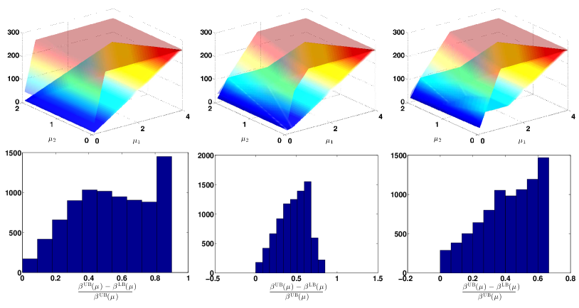
Figure 1: Certified NNSCM for the first test problem. Plotted on the first row are the lower bounds and upper bounds (as functions of the parameter) after the $1^{\rm st}$, $2^{\rm nd}$, and $3^{\rm rd}$ (final) round of domain decomposition. On the bottom row is the histogram of ${\frac{\beta^{\rm UB}({\boldsymbol{\mu}})-\beta^{\rm LB}({\boldsymbol{\mu}})}{\beta^{\rm UB}({\boldsymbol{\mu}})}}$. Their maximums are $0.9,0.85,0.67$ from left to right. Notice that the original NNSCM would have stopped after the first column.

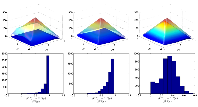
Figure 2: Certified NNSCM for the second test problem. Plotted on the first row are the lower bounds and upper bounds (as functions of the parameter) after the $1^{\rm st}$, $4^{\rm th}$, and $6^{\rm th}$ (final) round of domain decomposition. On the bottom row is the histogram of ${\frac{\beta^{\rm UB}({\boldsymbol{\mu}})-\beta^{\rm LB}({\boldsymbol{\mu}})}{\beta^{\rm UB}({\boldsymbol{\mu}})}}$. Their maximums are $0.99986,0.943,0.761$ from left to right. Notice that the original NNSCM would have stopped after the first column.

6 Concluding remarks

A rigorous and controllably tight lower bound for the stability parameter that is efficiently achievable is a critical part in the development of certified reduced basis methods for parametrized partial differential equations. The available methodologies either suffer from significant computational cost or inferior tightness of the bound.

In this paper, we have improved a recent novel approach combining two previous techniques by adding a mechanism through which the practitioners can control the tightness of the lower bound. It is achieved by building simultaneously an upper bound and shrinking the gap between the two through multiple domain decompositions. Numerical experiments demonstrate the effectiveness of the new approach and highlight its significant improvement over the Natural-Norm SCM.

References

- [1] R.A. Adams. Sobolev Spaces. Pure and applied mathematics. Academic Press, 1975.
- [2] B. O. Almroth, P. Stern, and F. A. Brogan. Automatic choice of global shape functions in structural analysis. AIAA Journal, 16:525–528, May 1978.
- [3] M. Barrault, N. C. Nguyen, Y. Maday, and A. T. Patera. An “empirical interpolation” method: Application to efficient reduced-basis discretization of partial differential equations. C. R. Acad. Sci. Paris, Série I, 339:667–672, 2004.
- [4] Y. Chen, J. S. Hesthaven, Y. Maday, and J. Rodríguez. A monotonic evaluation of lower bounds for inf-sup stability constants in the frame of reduced basis approximations. C. R. Acad. Sci. Paris, Ser. I, 346:1295–1300, 2008.
- [5] Y. Chen, J. S. Hesthaven, Y. Maday, and J. Rodríguez. Improved successive constraint method based a posteriori error estimate for reduced basis approximation of 2d maxwell’s problem. M2AN, 43:1099–1116, 2009.
- [6] S. Deparis. Reduced basis error bound computation of parameter-dependent navier-stokes equati the natural norm approach. SIAM J. Numer. Anal., 46(4):2039–2067, 2008.
- [7] J. P. Fink and W. C. Rheinboldt. On the error behavior of the reduced basis technique for nonlinear finite element approximations. Z. Angew. Math. Mech., 63(1):21–28, 1983.
- [8] M. A. Grepl, Y. Maday, N. C. Nguyen, and A. T. Patera. Efficient reduced-basis treatment of nonaffine and nonlinear partial differential equations. Mathematical Modelling and Numerical Analysis, 41(3):575–605, 2007.
- [9] B. Haasdonk, M. Ohlberger. Reduced basis method for finite volume approximations of parametrized linear evolution equations. M2AN Math. Model. Numer. Anal. 42: 277–302, 2008.
- [10] D.B.P. Huynh, D.J. Knezevic, Y. Chen, J.S. Hesthaven, and A.T. Patera. A natural-norm successive constraint method for inf-sup lower bounds. CMAME, 199:1963–1975, 2010.
- [11] D.B.P. Huynh, G. Rozza, S. Sen, and A.T. Patera. A successive constraint linear optimization method for lower bounds of parametric coercivity and inf-sup stability constants. C. R. Acad. Sci. Paris, Srie I., 345:473 – 478, 2007.
- [12] L. Machiels, Y. Maday, I. B. Oliveira, A. T. Patera, and D. V. Rovas. Output bounds for reduced-basis approximations of symmetric positive definite eigenvalue problems. C. R. Acad. Sci. Paris Sér. I Math., 331(2):153–158, 2000.
- [13] Y. Maday. Reduced basis method for the rapid and reliable solution of partial differential equations. In International Congress of Mathematicians. Vol. III, pages 1255–1270. Eur. Math. Soc., Zürich, 2006.
- [14] Y. Maday, A. T. Patera, and D. V. Rovas. A blackbox reduced-basis output bound method for noncoercive linear problems. In Nonlinear partial differential equations and their applications. Collège de France Seminar, Vol. XIV (Paris, 1997/1998), volume 31 of Stud. Math. Appl., pages 533–569. North-Holland, Amsterdam, 2002.
- [15] N.C. Nguyen, K. Veroy, and A. T. Patera. Certified real-time solution of parametrized partial differential equations. In Sidney Yip, editor, Handbook of Materials Modeling, pages 1529–1564. Springer Netherlands, 2005.
- [16] A. K. Noor and J. M. Peters. Reduced basis technique for nonlinear analysis of structures. AIAA Journal, 18(4):455–462, April 1980.
- [17] T. A. Porsching. Estimation of the error in the reduced basis method solution of nonlinear equations. Math. Comp., 45(172):487–496, 1985.
- [18] C. Prud’homme, D. Rovas, K. Veroy, Y. Maday, A. T. Patera, and G. Turinici. Reliable real-time solution of parametrized partial differential equations: Reduced-basis output bound methods. Journal of Fluids Engineering, 124(1):70–80, March 2002.
- [19] A. Quarteroni and A. Valli. Numerical Approximation of Partial Differential Equations. Springer Series in Computational Mathematics. Springer, 2008.
- [20] G. Rozza, D.B.P. Huynh, and A.T. Patera. Reduced basis approximation and a posteriori error estimation for affinely parametrized elliptic coercive partial differential equations: Application to transport and continuum mechanics. Arch Comput Methods Eng, 15(3):229–275, 2008.
- [21] S. Sen, K. Veroy, D.B.P. Huynh, S. Deparis, N.C. Nguyen, and A.T. Patera. “Natural norm” a posteriori error estimators for reduced basis approximations. J. Comput. Phys., 217(1):37 – 62, 2006.
- [22] L. N. Trefethen. Spectral methods in MATLAB, volume 10 of Software, Environments, and Tools. Society for Industrial and Applied Mathematics (SIAM), Philadelphia, PA, 2000.
- [23] S. Vallagh, A. Le Hyaric, M. Fouquembergh, and C. Prud’homme. A successive constraint method with minimal offline constraints for lower bounds of parametric coercivity constant. Preprint: hal-00609212, hal.archives-ouvertes.fr
- [24] S. Zhang. Efficient greedy algorithms for successive constraints methods with high-dimensional parameters. Brown Division of Applied Math Scientific Computing, Tech Report, 23, 2011.