Circular Hall Effect in a wire

Abstract

A constant longitudinal current in a wire is accompanied by azimuthal magnetic field. In absence of the radial current in a wire bulk the nonzero radial(Hall) electric field must be present. The longitudinal current can be viewed as collective drift of carriers in crossed magnetic(azimuthal) and electric(radial) fields, hence can be ascribed as Circular Hall Effect. At low temperatures the enhanced carrier viscosity leads to nonuniform current density whose radial profile is sensitive to presence of $collinear$ diamagnetic currents nearby the wire inner wall. Both the current and azimuthal magnetic field are squeezed out from the bulk towards the inner wall of a wire. Magnetic properties of a sample resembles those expected for ideal diamagnet. At certain critical temperature a former dissipative current becomes purely diamagnetic providing the zero resistance state. At low currents the temperature threshold is found for arbitrary disorder strength and the sample size. For bulky sample and finite currents the threshold temperature is found as a function of the magnetic field.

I Introduction

Usually, the Hall measurementsHall1879 imply the presence of external magnetic field source. Evidence shows that the current itself produces a finite magnetic field which may, in turn, influence the current carrying state. In the present paper, we take the interest in a special case when the only current-induced magnetic field is present. Therefore, we reveal a Circle Hall Effect in a round cross section conductor. The account of finite carrier viscosity and diamagnetic currents at the inner boundary of the wire provides a certain feasibility of the zero resistance state at low temperatures.

II Circular Hall Effect: uniform current flow

The conventional Drude equation for 3D electrons placed in arbitrary electric $\mathbf{E}$ and magnetic $\mathbf{B}$ fields yields

$$\frac{\partial\mathbf{V}}{\partial t}=\frac{e\mathbf{E}}{m}+\left[\mathbf{V}\times\mathbf{\Omega}_{c}\right]-\frac{\mathbf{V}}{\tau},\\$$ (1)

where $e$ is absolute value of the electric charge, $\mathbf{\Omega}_{c}=\frac{e\mathbf{B}}{mc}$ is the cyclotron frequency vector, $m$ is the effective mass, $\tau$ is the momentum relaxation time due to collisions with impurities and(or) phonons, $\mathbf{V}$ is the carrier flux velocity.

For steady state one obtains the following equation

$$\mathbf{V}=\mu\mathbf{E}+\left[\mathbf{V}\times\mathbf{\Omega}_{c}\tau\right],\\$$ (2)

where $\mu=\frac{e\tau}{m}$ is the carrier mobility. For arbitrary orientation of the electric and the magnetic fields the exact solution of Eq.(2) is straightforward Anselm78 .

Let us restrict ourself to a wire of radius $R_{0}$ and, hence use the cylindrical geometry frame. The voltage source(not shown in Fig.1) is attached to a free wire ends providing the longitudinal electric field $E_{z}$. The carrier velocity $v_{z}$ is uniform. Following to Biot-Savart law the longitudinal current density $j_{z}=neV_{z}$ results in azimuthal magnetic field $B_{\varphi}=\frac{2\pi j_{z}}{c}R$, where $R$ is the radial coordinate, $n$ is the carried density. The azimuthal magnetic field reaches the maximal value $B_{0}=B_{\varphi}(R_{0})$ at the rod wall. Note that the radial current is absent in the sample bulk. Hence, the nonzero radial electric field $E_{R}$ must exist to prevent Lorentz force $\sim V_{z}B_{\varphi}/c$ action. Evidently, the radial electric field plays the role of Hall one regarding conventional descriptionHall1879 .

Following the above reasoning we re-write Eq.(2) for both the longitudinal $v_{z}$ and radial $v_{r}=0$ components of the carrier velocity as it follows:

$$V_{z}=\mu E_{z},$$ (3)

$$V_{z}=c\frac{E_{R}}{B_{\varphi}}.$$ (4)

Eq.(3) provides a familiar differential Ohm’s law. By contrast, Eq.(4) presents the novel view on the longitudinal current as a carriers drift in crossed $E_{R}\perp B_{\varphi}$ fields, i.e. ascribes a Circular Hall Effect. We argue that the radial electric field $E_{R}=2\pi neR\left(\frac{V_{z}}{c}\right)^{2}$ defines volumetric charge density $Q=\text{div}\mathbf{E}/4\pi=ne\left(\frac{V_{z}}{c}\right)^{2}$. Thus, the wire is chargedMatzek68 ; McDonald2010 since $Q/ne\ll 1$.

Figure 1: Schematic view of the Circular Hall effect.

III Circular Hall Effect: Nonuniform viscose flow

We now intend to answer a question whether the current carrying state in a wire can be nonuniform in radial direction, namely $V_{z}(R)$. Navier-Stokes equation modified with respect to presence of the magnetic field yields

$$\frac{\partial\mathbf{V}}{\partial t}+(\mathbf{V}\nabla)\mathbf{V}=\frac{e\mathbf{E}}{m}+\left[\mathbf{V}\times\mathbf{\Omega}_{c}\right]+\hat{\eta}\triangle\mathbf{V}-\frac{\mathbf{V}}{\tau}.\$$ (5)

Here, $\hat{\eta}$ is the viscosity tensorSteinberg58 ; Alekseev16 whose longitudinal and transverse components

$$\eta_{xx}=\eta_{yy}=\frac{\eta}{1+4\Omega_{c}^{2}\tau_{ee}^{2}},$$ (6)

$$\eta_{xy}=-\eta_{yx}=\eta_{xx}2\Omega_{c}\tau_{ee}$$

depend on magnetic field. Then, $\eta=\frac{1}{5}v^{2}_{F}\tau_{ee}$ is the kinematic viscosity of the carriers at zero magnetic field, $V_{F}$ is the Fermi velocity, $\tau_{ee}$ is the electron-electron collisions time. Viscosity effects become importantGurzhi63 when the e-e mean free path $l_{ee}=V_{F}\tau_{ee}$ is less and(or) comparable to that caused by phonons and(or) impurities $l=V_{F}\tau$ and typical length scale of the sample. Note that under assumption of radially dependent velocity $V_{z}(R)$ the Euler term can be neglected in Eq.(5).

For steady state Eq.(5) can be re-written for both the longitudinal and radial components of carrier velocity as it follows

$$\eta_{xx}\tau\triangle_{R}V_{z}-V_{z}+\mu E_{z}=0,$$ (7)

$$\eta_{yx}\triangle_{R}V_{z}+\frac{eE_{R}}{m}-\frac{V_{z}eB_{\varphi}}{mc}=0.$$ (8)

Here, $\triangle_{R}=\frac{1}{R}\frac{d}{dR}\left(R\frac{d}{dR}\right)$ is the radial component of the Laplace operator. Our primary interest concerns Eq.(7) which determines the nonuniform velocity profile $V_{z}(R)$ and, in turn, the azimuthal magnetic field

$$B_{\varphi}=\frac{4\pi ne}{cR}\int\limits^{R}_{0}V_{z}(R)RdR.\$$ (9)

Introducing the dimensionless velocity $v=V_{z}(R)/\mu E_{z}$ and the reduced radius $r=R/R_{0}$, one may rewrite Eq.(7) as it follows

$$\frac{\eta_{xx}}{\eta}\nu^{-2}\triangle_{r}v-v+1=0.\\$$ (10)

where $\nu=R_{0}/\lambda$ is the dimensionless parameter, $\lambda=\sqrt{\eta\tau}$ is the typical length scale of the problem. The condition $\nu\ll 1$( $\nu\gg 1$ ) determines the high(low)-viscous electron gas respectively.

We argue the solution of Eq.(10) is complicated due to magnetic field dependent longitudinal viscosity. In principle, Eq.(10) can be expressed in terms of the reduced magnetic field $B_{\varphi}/B_{0}$ via relationship $v=\frac{1}{2r}\frac{d}{dr}(rB_{\varphi}/B_{0})$ but still remains difficult for analytical processing. Fortunately, at small currents and(or) small magnetic fields $\Omega_{c}\tau_{ee}\ll 1$ the longitudinal viscosity can be kept constant $\eta_{xx}\sim\eta$, thus Eq.(10) becomes amenable for analytic analysis. Noteceably, at low magnetic fields the transverse viscosity can be disregarded in Eq.(8) which, in turn, gives a familiar result for carrier drift in crossed $E_{R}\perp B_{\varphi}$ fields.

Under the above assumptions the solution of Eq.(7) is straightforward:

$$v(r)=1+C_{1}J_{0}(\nu r)+C_{2}Y_{0}(\nu r),\\$$ (11)

where $J_{0}$ and $Y_{0}$ are zero-order modified Bessel functions of the first and second kind respectively. Since the carrier velocity remains always finite, we conclude that $C_{2}=0$, because $Y_{0}\rightarrow\infty$ at $r\rightarrow 0$. Introducing a general condition $v|_{R=R_{0}}=v_{0}$ for longitudinal velocity at the inner wire wall Eq.(11) yields

$$v(r)=1+(v_{0}-1)\frac{J_{0}\left(\nu r\right)}{J_{0}(\nu)},\\$$ (12)

Note that the trivial case of the uniform current flow examined in Sec.II follows from Eq.(12) when $v_{0}=1$. We now demonstrate that the boundary condition at the inner wire surface alters crucially the radial velocity profile and, moreover, the sample resistivity.

III.1 Poiseuille viscose flow

We recall that the simple wall adhesion condition $v_{0}=0$ Gurzhi63 could be familiar regarding the Poiseuille’s viscous flow in conventional hydrodynamics. In Fig.2 the blue curves depict the radial dependence of the flux velocity $v(r)$ specified by Eq.(12) for different viscosity strengths. As expected, for small viscosity $\nu\gg 1$ the 3D fluid velocity is mostly uniform with exception of ultra-narrow layer $\sim\lambda$ close to wire inner wall. In contrast, for highly viscous case $\nu\leq 1$ the flux velocity follows the Poiseuille law $v(r)=\frac{\nu^{2}}{4}(1-r^{2})$ shown by the dashed line in Fig.2.

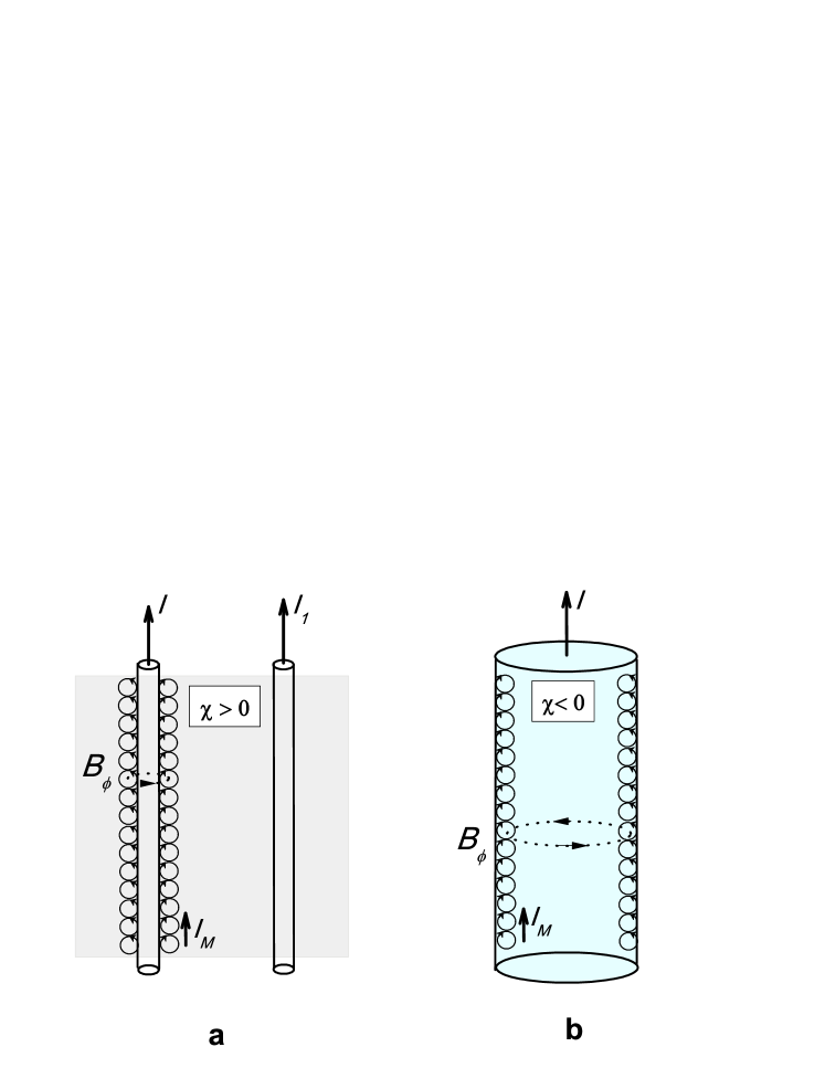
Figure 2: The microscopic magnetic currents for a) current carrying conductors placed into paramagnetic $\chi>0$ media ( from Ref.Sivukhin96 ) b) The sole current carrying diamagnetic $\chi<0$ conductor.

III.2 Diamagnetic viscose flow

The special interest of the present paper concerns the possibility of different boundary condition $v_{0}>1$ whose physical background we intend to illustrate hereafter.

At first, recall a scenario of a current carrying wire surrounded by paramagnetic media(see the left-hand sketch in Fig.2,a). Let the longitudinal current $I$ is provided by an external source. The current carrying wire induces the azimuthal magnetic field $B_{\varphi}=\frac{2I}{cR}$ in the surrounding space $R>R_{0}$. Notably, the magnetic field at the outer wire wall $B_{0}=B_{\varphi}(R_{0})$ results in nonzero microscopic magnetic current $I_{M}=4\pi\chi I$Sivukhin96 ; Vlasov05 because of the paramagnetic surrounding. Here, $\chi>0$ is the paramagnetic susceptibility. The total current flowing along the wire yields $I+I_{M}$. Let an another conductor with a driven current $I_{1}$( see Fig. 2,a ) is placed in parallel to initial one. Again, the total current along the second wire $(1+4\pi\chi)I_{1}$ includes a microscopic component(not shown in Fig. 2,a) as well. One can check that Ampere’s attractive force $\sim(1+4\pi\chi)I\cdot I_{1}$ between a pair of wires with parallel currents is enhanced by a factor of $1+4\pi\chi$Sivukhin96 compared to that in absence of paramagnetic media. We conclude that Ampere’s force enhancement is caused by microscopic magnetic currents at the outer wire surface.

We now provide a strong evidence of similar effect for current carrying diamagnetic wire $\chi<0$, shown in Fig.2,b. Indeed, for certain value of the applied current $I$ the azimuthal magnetic field at the inner rod surface $B_{0}$ results in extra diamagnetic current $I_{M}$ which is parallel to native current, namely $I_{M}=4\pi|\chi|I$. Phenomenologically, we assume that diamagnetic current may flow within narrow layer of the width $\delta$. The respective density of diamagnetic current $j_{M}=\frac{I_{M}}{2\pi R_{0}\delta}$ may exceed the ohmic current density $j_{z}$. One can deduce the dimensionless flux velocity $v_{0}$ at the inner rod surface as

$$v_{0}=\frac{j_{M}}{j_{z}}=\frac{j}{j_{z}}\kappa,\\$$ (13)

where we introduced the average current density $j=\frac{I}{\pi R_{0}^{2}}$ while $j_{z}=ne\mu E_{z}$ is the ohmic current density. Then, $\kappa=\frac{2\pi R_{0}|\chi|}{\delta}$ is the dimensionless diamagnetic parameter dependent on the sample size. Without diamagnetic currents, i.e. when $\kappa=0$ we recover the conventional Poiseille’s flow provided by the wall-adhesion condition $v_{0}=0$.

Our major interest concerns a strong diamagnetism case when $\kappa\geq 1$. In Fig.3 we plot the radial distribution of longitudinal velocity at fixed boundary velocity $v_{0}=4$ and different strengths of the carrier viscosity. As expected, the diamagnetic current within a narrow layer $\delta$ initiates a current flow within in much wider stripe $\lambda\gg\delta$ close to sample inner wall. The flux velocity approaches a conventional ohmic drift velocity in a sample bulk.

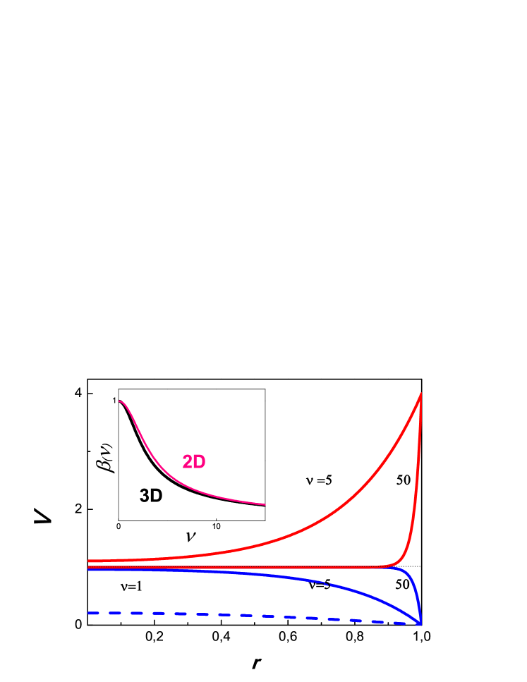
Figure 3: Flux velocity distribution $v(r)$ specified by Eq.(12) at fixed applied longitudinal electric field and viscosity parameter $\nu=5;50$ for wall adhesion boundary condition $v_{0}=0$(blue) and diamagnetic boundary condition $v_{0}=4$(red). The Poiseuille flow for $v_{0}=0;\nu=1$ is shown by the dashed line. Dotted line represents the uniform flow $v=v_{0}=1$. Inset: universal dependence $\beta(\mu)$ for present 3D wire case. Pink curve $\beta_{2D}(\mu)$ corresponds to 2D slab case discussed in text.

Using Eq.(12) one may find the average current density $j=\frac{2ne}{R_{0}^{2}}\int\limits^{R_{0}}_{0}V_{z}(R)RdR$:

$$j=j_{z}\left[1+(v_{0}-1)\beta(\nu)\right],\\$$ (14)

where $\beta(\nu)=\frac{2J_{1}(\nu)}{\nu J_{0}(\nu)}$ is the universal function(see Fig.3,inset) of the viscosity strength, $J_{1}$ is first-order modified Bessel function of the first kind. The function $0<\beta(\nu)\leq 1$ decreases smoothly as $\sim 1-\nu^{2}/8$ for high-viscous case $\nu\ll 1$ and, then follows the asymptote $\sim 2/\nu$ for low viscosities $\nu\gg 1$.

Remarkably, the all previous arguments can be generalize for two-dimensional slab whose thickness is much less compared to other sample sizes. Actually, 2D slab thickness plays the role of a wire radius upon straightforward replacement in present notations. We find that for 2D slab geometry the universal function $\beta(\nu)$ can be replaced by $\beta_{2D}(\mu)=2\tanh(\nu)/\nu$ shown by pink line in Fig.3,inset. Both dependencies are close one to each other, therefore we expect a similar effects which will be discussed hereafter. The detailed analysis of 2D slab case will be available elsewhere.

From Eq.(13) the self-consistent solution of Eq.(14) yields

$$j=j_{z}\frac{1-\beta}{1-\kappa\beta}.\\$$ (15)

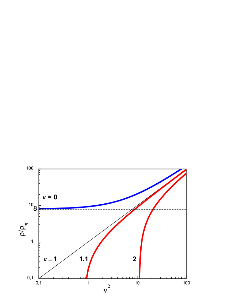
Figure 4: Dimensionless resistivity $\rho/\rho_{\eta}$ followed from Eq.(16) vs dimensionless disorder strength $\nu^{2}=\frac{R_{0}^{2}}{\eta\tau}$ for: zero diamagnetic current $\kappa=0$; uniform current state $\kappa=1$; strong diamagnetism $\kappa>1$. Dashed line represents the viscous resistivity $\rho=8\rho_{\eta}$ at $\kappa=0$ and $1/\tau\rightarrow 0$.

Eq.(15) defines the average current density at fixed longitudinal electric field $E_{z}$. Consequently, one may define the ”effective resistivity” $\rho=E_{z}/j$ as it follows

$$\rho=\rho_{D}\frac{1-\kappa\beta}{1-\beta},\\$$ (16)

where $\rho_{D}=\frac{m}{ne^{2}\tau}$ is the conventional Drude resistivity.

Eq.(16) represents the central result of the paper. The galvanic measurements give the ”effective resistivity” which depends on the inner wall boundary condition, sample size and, moreover, differs from expected Drude value. At first, for $\kappa=1$ one recover the uniform current flow without viscous effects, hence $\rho=\rho_{D}$. Secondly, the wall adhesion condition $\kappa=0$ provides the ”effective resistivity” as $\rho=\rho_{D}/(1-\beta)$ already reported in Ref.Gurzhi63 . For low-viscose case $\nu\gg 1$ the ”effective resistivity” is still described by Drude formulae $\rho\sim\rho_{D}$. In the opposite high-viscosity and(or) low dissipation limit $\nu\ll 1$ the Poiseille type of a current flow is realized. The ”effective resistivity” at $\nu\ll 1$ is given by the asymptote $\rho=8\rho_{\eta}$, where $\rho_{\eta}=\frac{m}{ne^{2}}\frac{\eta}{R_{0}^{2}}$ is so-called ”viscous” resistivityGurzhi63 which depends on the sample size. Note, the ratio $R_{0}^{2}/\eta$ plays the role of the momentum relaxation time similar to that discussedAlekseev16 ; Shi14 for 2D electron gas. The transition from Drude to ”viscous” resistivity case occurs at $\nu\sim 1$.

In Fig.4 we plot the reduced resistivity $\rho/\rho_{\eta}$ vs disorder $\nu^{2}\sim 1/\tau$ for fixed viscosity strength $\eta$ and different valued of diamagnetic parameter $\kappa$. Note that at high disorder and(or) low viscosity $\nu\gg 1$ the resistivity in Fig.4 starts to follow conventional Drude dependence. The most intriguing feature of Eq.(16) concerns the effective resistivity which may vanish at

$$\kappa\cdot\beta(\nu)=1.\\$$ (17)

Eq.(17) gives the critical condition for so-called ”zero-resistance state” (ZRS) seems to be observed in Ref.Kamerlingh-Onnes1911 . Recall that for arbitrary argument $\beta(\nu)\leq 1$. Thus, the solution of transcendental Eq.(17) is possible when $\kappa>1$. The condition $\kappa>1$ can be re-written as $R_{0}\geq R_{m}$, where we introduce the minimal wire radius

$$R_{m}=\frac{\delta}{2\pi|\chi|},\\$$ (18)

when the ZRS can be realized. We further demonstrate that ZRS criteria $\kappa=R_{0}/R_{m}>1$ could be even stronger regarding real systems.

We emphasize that the zero resistance state may appear for even finite momentum relaxation time. At a first glance, this result looks like mysterious. Nevertheless, the experimental dataMeissner32 provide a strong evidence of the disorder remains indeed finite within zero-resistance state. We argue that the physics of zero-resistance state is rather transparent. The non-dissipative diamagnetic current is pinched within a narrow inner layer $\lambda\sim R_{m}/2$ of a wire and, then shunts the dissipative current in the sample bulk. The total current in a wire becomes purely diamagnetic when Eq.(17) is fulfilled.

III.3 Size-dependent transition to zero-resistance state

We now examine in greater details the critical condition given by Eq.(17). One can find, in principle, the critical dependence in a following form $\nu^{cr}(\kappa)$. The latter is, however, non-informative since both variables $\kappa,\nu$ depend on the sample size. To avoid this problem, let us introduce a size-free parameter $z=\frac{\nu}{2\kappa}=\frac{R_{m}}{2\lambda}$. The modified Eq.(17) yields the transcendental equation

$$z=\frac{J_{1}(2\kappa z)}{J_{0}(2\kappa z)}.\\$$ (19)

which gives a desired critical diagram in a form $z^{cr}(\kappa)$. The latter is shown in Fig.5,a. Again, the area below the critical curve corresponds to zero resistance state. For sample size closed to its minimal value $R_{m}$, i.e. when $\kappa-1\ll 1$, the critical curve follows the asymptote $z^{cr}=\sqrt{2(\kappa-1)}$ depicted by the dashed line in Fig.5,a. Then, the critical curve saturates asymptotically as $z^{cr}(\kappa)=1-\frac{1}{4\kappa}$ for bulky sample, i.e. when $\kappa\gg 1$.

Up to this moment we assumed the momentum relaxation time and the carrier viscosity to be temperature independent. One can make an attempt to find ZRS threshold in terms of temperature since $z\sim 1/\lambda=1/\sqrt{\eta\tau}$. Remind that for actual low-T case the transport is mostly governed by scattering on static defects, hence one may consider the T-independent momentum relaxation time $\tau\neq\tau(T)$. In contrast, the e-e scattering time is knownPomeranchuk50 ; Abrikosov59 ; Baym67 to be a strong function of temperature. Thus, we assign

$$\frac{1}{\tau_{ee}(T)}=\frac{\xi^{2}}{\tau^{1}_{ee}}+\frac{1}{\tau^{0}_{ee}},\\$$ (20)

where $\xi=T/T_{F}$ is the degeneracy parameter, $T_{F}=\varepsilon_{F}/k$ and $\varepsilon_{F}$ are the Fermi temperature and energy respectively. Then, $\tau^{0}_{ee}$ is the residual value of e-e scattering time at $T\rightarrow 0$, $\tau^{1}_{ee}$ is a dimensional value known to be of the order of $\hbar/\varepsilon_{F}$ within Fermi liquid theoryPines96 . In general, both values $\tau^{0,1}_{ee}$ are unknown, thus stay to be extracted from experimental data.

Figure 5: a) The critical diagram $z^{cr}(\kappa)$ of zero-resistance state followed from Eq.(19). The asymptotes for small $\kappa-1\ll 1$ and bulky sample $\kappa\gg 1$ are shown by dashed and dotted line respectively. The area below the critical curve $z^{cr}(\kappa)$ corresponds to zero-resistance state. b) The dependence $z(\Theta)$ specified by Eq.(26). c) The resulting temperature threshold dependence $\Theta(\kappa)$ specified by Eq.(27) for fixed $z_{m}=0.7$.

With the help of Eq.(20) the parameter $z=\frac{R_{m}}{2\lambda}$ becomes temperature dependent, namely

$$z(\xi)=z_{m}\sqrt{1+\gamma\xi^{2}},\\$$ (21)

where $\gamma=\tau^{0}_{ee}/\tau^{1}_{ee}$ is the dimensionless ratio, then $z(0)=z_{m}=\frac{\sqrt{5}R_{m}}{2v_{F}\sqrt{\tau^{0}_{ee}\tau}}$ is the zero temperature value. Recall that $z^{cr}(\kappa)\leq 1$, hence a condition $z_{m}\leq 1$ must be satisfied. The latter gives the condition

$$\mu\geq\mu_{\text{min}},\\$$ (22)

for carrier mobility, where $\mu_{\text{min}}=\frac{5}{8}\frac{eR_{m}^{2}}{\varepsilon_{F}\tau^{0}_{ee}}$ plays the role of the minimal mobility for which the ZRS is possible. Further, we will use a trivial relationship $z_{m}=\sqrt{\mu_{\text{min}}/\mu}$ as well.

If $z_{m}<1$, the only upper part $z^{cr}(\kappa)>z_{m}$ of the threshold diagram in Fig.5,a remains useful. Then, the equality $z_{m}=z^{cr}(\kappa_{m})$ denotes a certain value of minimal sample size parameter $\kappa_{m}$, which corresponds to ZRS threshold at $T=0$. Evidence shows that at finite temperature the zero resistance state can be realized for samples whose sizes satisfy the condition $\kappa\geq\kappa_{m}$. The latter gives the strict criteria

$$R_{0}\geq R_{m}\cdot\kappa_{m}\\$$ (23)

for minimal sample radius instead of that $R_{0}\geq R_{m}$ discussed earlier.

We now attempt to find out the threshold temperature for massive sample( i.e. when $\kappa\gg 1$ ) known to be a universal quantityKamerlingh-Onnes1911 for certain material. Helpfully, it can be done within our model. Indeed, with the help of Eq.(21) and condition $z(\xi)=1$ valid for massive sample one obtains the subsequent threshold temperature $T_{c}$:

$$T_{c}=T_{F}\left[(z^{-2}_{m}-1)/\gamma\right]^{1/2}.\\$$ (24)

Hereafter, we will label the all quantities related to ZRS threshold in bulky sample by index ”c”. Remarkably, one may re-write Eq.(24) in terms of resistivity $\rho_{c}=\rho|_{T_{c}}$ associated with the critical temperature $T_{c}$:

$$\frac{\rho_{c}}{\rho_{\text{max}}}=\frac{1}{1+\gamma(T_{c}/T_{F})^{2}},\\$$ (25)

where we use a notation $\rho_{\text{max}}=(ne\mu_{\text{min}})^{-1}$. Let us assume a pure massive sample exhibited a certain ZRS threshold point at $\rho_{c},T_{c}$. The momentum relaxation time may depend on static disorder. Eq.(25) provides an evidence of ZRS threshold temperature decay caused by disorder enhancement. These predictions is qualitatively confirmed by experimental observationsLynton57 .

It is useful to introduce the reduced temperature $\Theta=T/T_{c}$. Consequently, Eq.(21) can be modified as it follows

$$z(\Theta)=\sqrt{z_{m}^{2}+(1-z_{m}^{2})\Theta^{2}},\\$$ (26)

and, then plotted in Fig.5,b. Combining the dependencies $z(\Theta)$ and $z^{cr}(\kappa)$ specified by Eq.(26) and Eq.(19) respectively one obtains threshold temperature as a function of the sample size $\Theta(\kappa)$:

$$\Theta(\kappa)=\left[\frac{z^{cr}(\kappa)^{2}-z^{2}_{m}}{1-z^{2}_{m}}\right]^{1/2}.\\$$ (27)

An example is shown in Fig.5,c. Experimentally, threshold temperature diminution was observedMeissner33 ; Meissner35 ; Burton34 for small sized samples.

Figure 6: a) Dependence $\rho_{c}(T_{c})$ specified by Eq.(25). Inset: sketch view of experimental resistivity curves $\rho(T)$ used to determine $\rho_{c}(T_{c})$.

Finally, we will explore our model in order to demonstrate a possibility of sample-size driven ZRS to normal metal transition. Let us consider a wire for which the zero-resistance state can be realized. For example, we assign $z_{m}=0.7<1$. With the help of critical diagram shown in Fig.5 we find the minimal value of diamagnetic parameter $\kappa_{m}=1.44$. Using Eq.(26) and, then substituting $\nu=2\kappa z(\Theta)$ into Eq.(16) one obtains T-dependent resistivity $\rho(\Theta)$ for fixed values of sample radius $\kappa=R_{0}/R_{m}$ . The result is shown in Fig.7. Evidence shows that the change from apparent ”metallic” $\frac{d\rho}{dT}>0$ to ”insulating” $\frac{d\rho}{dT}<0$ behavior occurs when $\kappa=1$, i.e. for uniform current flow regime. We claim that the key parameter $R_{m}$ can be amenable for experimental test regarding divergent $\rho(T)$-data analysis.

Figure 7: a) Resistivity set $\rho(\Theta)$ for sample-size driven ZRS-to-normal state transition for $z_{m}=0.7$ and $k=R_{0}/R_{m}=30;2;k_{m}=1.438;1.3;1.1;1;0.9;0.7;0.4$(from bottom to top).

III.3.1 Proximity Effect

In general, the experimental observation of the proposed size-dependent threshold transition could be rather difficult since it requires a typical wire radius of the order of hundred angstroms. To avoid this problem the authors of Refs.Burton34 ; Misener35 ; Hilsch62 suggested a coaxial construction of normal metal kernel( see Fig.8a, inset ) of a fixed radius coated by Pb-superconductor layer of angstrom scale width $d\ll R_{0}$. The layer width $d$ can be varied. In Fig.8b we reproduce the critical temperature $T(d)$ dataHilsch62 for coaxial sample. The superconducting state occurs when the coating width exceeds a certain minimal value $d_{0}$. We now demonstrate that this result can be easily obtained within our model. Indeed, we reproduce the all previous calculations for coaxial geometry and, then obtain the following equation

$$z=\frac{Y_{0}(\nu\Delta)\left[J_{1}(\nu)-\Delta J_{1}(\nu\Delta)\right]+J_{0}(\nu\Delta)\left[Y_{1}(\nu)-\Delta Y_{1}(\nu\Delta)\right]}{Y_{0}(\nu\Delta)J_{0}(\nu)-Y_{0}(\nu)J_{1}(\nu\Delta)},\\$$ (28)

where $\Delta=1-d/R_{0}$ is the dimensionless ratio of the inner core radius to $R_{0}$, then $Y_{1}$ is the first-order modified Bessel function of the second kind. Surprisingly, Eq.(28) does not contain any component caused by dissipative current inside the metallic core. We find that even the kernel is empty the Eq.(28) remains unchanged. Indeed, our previous findings specified by Eq.(19) deals with a purely non-dissipative diamagnetic current flow in a narrow layer nearby the inner wall of a wire. The all dissipative currents can be disregarded in this respect. The same reasoning is valid for present case of coaxial sample with(without) the normal metal inside the core. Therefore, Eq.(28) is universal.

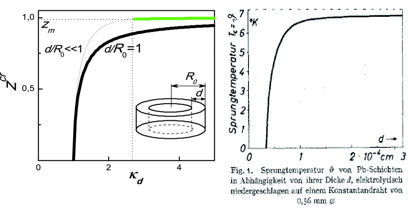
Figure 8: a) The critical diagram $z^{cr}(\kappa_{d})$ followed from Eq.(28) for solid wire $d/R_{0}=1$ and thin coating layer $d/R_{0}\ll 1$. Green curve depicts the experimental data in the panel b. Insert: coaxial sample geometry. b) Critical temperature vs Pb layer thickness for fixed inner core radius $0.28\text{mm}$ under Ref.Hilsch62 .

For fixed value of the core radius $\Delta\cdot R_{0}$ the solution of Eq.(28) provides a set of critical diagram curves $z^{cr}(\kappa_{d})$. Here, we make use of the dimensionless Pb-layer width $\kappa_{d}=d/R_{m}$ similar to variable $\kappa$ used above for simple wire case. The result is shown in Fig.8a. The zero-resistance state is possible when $\kappa_{d}>1$. For coreless wire $\kappa_{d}\rightarrow\kappa$ we readily reproduce the critical diagram shown previously in Fig.5. In the opposite case of massive core coated by a thin layer, i.e. when $d/R_{0}\ll 1$, the critical diagram is upshifted( see Fig.8a).

We now compare our model finding with experimentHilsch62 . Note that the present critical diagram $z^{cr}(\kappa_{d})$ can be used to deduce the critical temperature dependence $\Theta(\kappa_{d})$ similar to that depicted in Fig.5b,c. On the contrary, one may use the experimental dependence $\Theta(d)$ and, then impose it to a appropriate curve on the threshold diagram set $z^{cr}(\kappa_{d})$.

Keeping $z_{m}$ and $R_{m}$ as a fitting parameters, we plot in Fig.8a the dimensionless replica of the experimental data shown in Fig.8b. For actual core radius $0.28$mm and minimal coating width $d_{0}=3500$AHilsch62 our best fit gives $z_{m}=0.99$ and $d_{0}/R_{m}=2.71$. Therefore, we obtain $R_{m}=1290$A.

III.4 Magnetic field screening

We now demonstrate that the magnetic field can be pushed out from the sample bulk as stronger as the system becomes closer to zero resistance state threshold. Remind that the flux velocity distribution specified by Eq.(12) was found under assumption of a fixed electric field $E_{z}$. Using Eq.(15) the later can be represented in terms of total current $I$. As a result, both the radial distribution of the current density $j_{z}(r)$ and the azimuthal magnetic field $B_{\varphi}(r)$ specified by Eqs.(12),(13) and Eq.(9) respectively yield

$$j_{z}(r)=j\left[\frac{1-\kappa\beta}{1-\beta}+\frac{\kappa-1}{1-\beta}\cdot\frac{J_{0}(r\nu)}{J_{0}(\nu)}\right],$$ ()

$$B_{\varphi}(r)=B_{0}\left[\frac{1-\kappa\beta}{1-\beta}r+\beta\cdot\frac{\kappa-1}{1-\beta}\cdot\frac{J_{1}(r\nu)}{J_{1}(\nu)}\right].$$

Remind that $j=\frac{I}{\pi R_{0}^{2}}$ is the average current density. As expected, for uniform flow $\kappa=1$ one obtains $j_{z}(r)=j$, $B_{\varphi}=B_{0}r$. Then, Eq.(() ‣ III.4) gives the correct values of the current density $j_{z}(1)=j\kappa$ and the magnetic field $B_{\varphi}(1)=B_{0}$ at the inner surface of the wire. We plot the dependencies given by Eq.(() ‣ III.4) in Fig.9. At fixed diamagnetic parameter $\kappa>1$ the growth of the fluid viscosity leads to progressive shift of the current towards the inner wall of the wire. Simultaneously, the magnetic field is pushed out from the sample bulk.

Remind that the typical length scale of viscose flow yields $\lambda=\sqrt{\eta\tau}=\frac{R_{m}}{2z}$. For bulky sample at ZRS threshold $z=1$ one obtains the screening length $\lambda=l_{B}=R_{m}/2$. As an example, we plot in Fig.9, inset the magnetic field screening asymptote $B_{\varphi}=B_{0}\exp\left({\frac{R-R_{0}}{l_{B}}}\right)$.

Our final remark concerns the presence of the radial electric field. With the help of Eq.(8) and Eq.(() ‣ III.4) we obtain $E_{R}=\frac{j_{z}(r)B_{\varphi}(r)}{nec}$. Following our previous arguments the longitudinal current in a sample bulk can be viewed as a carriers drift in a crossed $E_{R}\perp B_{\varphi}$ fields.

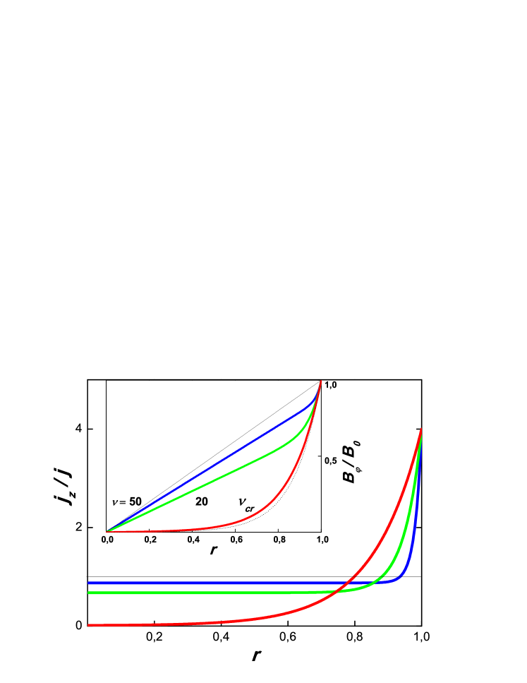
Figure 9: Distribution of the dimensionless current density $j_{z}/j$ and azimuthal magnetic field $B_{\varphi}/B_{0}$ (insert) specified by Eq.(() ‣ III.4) for finite size sample at $\kappa=4$(corresponds to $z_{cr}=0.93$ and $\nu_{cr}=2\kappa z_{cr}=7.44$) and viscosity parameter $\nu=\nu_{cr};20;50$. Thin lines depict the uniform current density case when $\kappa=1$. Dotted line(insert) corresponds to magnetic field screening asymptote described in text.

III.5 Magnetic field phase diagram of zero-resistance state

Remind that the all previous discussion concerned the zero-current limit of the transport measurements. The critical diagram of zero-resistance state was found for arbitrary sample size. In reality, a finite applied current and, hence accompanied current-induced azimuthal magnetic field are knownMeissner33 ; Meissner33+ ; Silsbee17 to influence threshold temperature of zero-resistance state. In order to account for current driven effects one must solve Eq.(10) modified with respect to magnetic field dependent longitudinal viscosity specified by Eq.(6). The resulting equation is rather difficult to be analytically resolved. However, one may qualitatively catch the underlying physics. For simplicity, we restrict ourself to massive sample case.

We re-write the threshold criteria given by Eq.(21) with carrier viscosity $\eta_{xx}$ included.

$$z(\xi,\Omega_{c})=z_{m}\sqrt{1+\gamma\xi^{2}}\sqrt{1+\frac{4\Omega_{c}^{2}(\tau_{ee}^{0})^{2}}{(1+\gamma\xi^{2})^{2}}}.\\$$ (29)

Note that within the above approach we neglect, in fact, the magnetic field radial distribution in a sample bulk.

To proceed, we write down a criteria $z(\xi,\Omega_{c})=1$ for massive specimen and obtain the threshold diagram in terms of the magnetic field vs temperature:

$$\frac{\Omega_{c}}{\Omega_{c}(0)}=\sqrt{(1-\Theta^{2})(1+(z_{m}^{-2}-1)\Theta^{2})}\\$$ (30)

where

$$\Omega_{c}(0)=\frac{\sqrt{z^{-2}_{m}-1}}{2\tau_{ee}^{0}}=\frac{1}{2\sqrt{\tau_{ee}^{0}\tau_{ee}^{1}}}\frac{T_{c}}{T_{F}}\\$$ (31)

is the cyclotron frequency and $B_{c}=mc\Omega_{c}(0)/e$ is the critical magnetic field respectively at $T\rightarrow 0$. Eq.(31) confirms the proportionality $B_{c}\sim T_{c}$ observed in experiment.

As an example, the magnetic field driven threshold diagram specified by Eq.(30) is plotted in Fig.10. The critical curve has a quadrant shape which is close to empiric dependence $B/B_{c}=1-\Theta^{2}$ often used in practice.

Figure 10: The critical magnetic field vs critical temperature specified by Eq.(30) for massive sample at $z_{m}=0.7;0.9$. The dashed curve corresponds to empirical dependence $B/B_{c}=1-\Theta^{2}$.

III.6 Estimations

For the sake of certainty, we further examine the massive lead whose typical low-T resistivity data dataClusius32 is represented in Fig.LABEL:Fig8. Let us use textbook valuesPool2007 of Fermi energy $\varepsilon_{F}=9.47$eV, velocity $v_{F}=1.83\times 10^{8}\text{cm/s}$ and carrier density $n=1.3\times 10^{23}\text{cm}^{-3}$ of a massive lead. At $T=273$K the typical resistivity is $\rho=1.9\times 10^{-7}\Omega\text{m}$Pool2007 . Hence, the low-T dataClusius32 denote the resistivity $\rho_{c}=3.8\times 10^{-10}\Omega\text{m}$ at ZRS threshold $T_{c}=7.2$K. The respective carrier mobility $\mu=1/(ne\rho_{c})=1240\text{cm}^{2}/\text{Vs}$ allows one to estimate the momentum relaxation time $\tau=7.1\cdot 10^{-13}\text{s}$ and the transport length $l=v_{F}\tau=1.3\mu\text{m}$. Using the above extracted value $z_{m}=0.99$ we calculate the minimal mobility as $\mu_{\text{min}}=\mu z^{2}_{m}=1215\text{cm}^{2}/\text{Vs}$. Our previous finding $R_{m}=1290$A gives the residual e-e scattering time $\tau^{0}_{ee}=\frac{5eR^{2}_{m}}{8\epsilon_{F}\mu_{\text{min}}}=0.9\cdot 10^{-14}\text{s}$. Then, we are able to calculate a ratio $\gamma=(z^{-2}_{m}-1)(T_{F}/T_{c})^{2}=4.7\cdot 10^{6}$ and, finally, deduce $\tau^{1}_{ee}=1.9\cdot 10^{-21}\text{s}$ imbedded into Eq.(20). Note that for actual temperatures $\sim T_{c}$ the total e-e scattering time specified by Eq.(20) is mostly determined by residual component, therefore $\tau_{ee}\sim\tau^{0}_{ee}$. The estimation of e-e scattering length $l_{ee}\sim v_{F}\tau^{0}_{ee}=0.02\mu\text{m}$ justifies the applicability of hydrodynamic approach since $l_{ee}\ll l$. It is instructive to find the magnetic filed penetration length at ZRS threshold as $l_{B}=R_{m}/2=640$A being of the order of magnitude of that $390$A known in literatureLynton1971 . Using Eq.(31) we find also the cyclotron frequency $\Omega_{c}(0)=7.8\times 10^{12}\text{c}^{-1}$ at $T\rightarrow 0$. The respective critical magnetic field $B_{c}=4.4\cdot 10^{5}$G is, however, much higher than that $\sim 803$G observed experimentally. We attribute the above discrepancy to approximate analytic approach used to find threshold criteria in presence of finite magnetic field.

Following Landau’s theory let us estimate the diamagnetic susceptibility of free electron gas $\chi=-\frac{1}{2}\frac{n\mu_{B}^{2}}{\varepsilon_{F}}=3.8\cdot 10^{-7}$, where $\mu_{B}=\frac{e\hbar}{2mc}$ is the Bohr’s magneton. The diamagnetic current is caused by movement of carriers on skipping orbits whose deviation from a sample wall $\delta=2\pi|\chi|R_{m}=4.6\cdot 10^{-13}$m is less than the average interelectronic distance $r_{s}=(4\pi n/3)^{-1/3}=1.2$A.

III.7 Conclusions

In conclusion, we discover the Circular Hall Effect in a wire taking into account both the diamagnetism and finite viscosity of 3D electron liquid. We demonstrate that under certain condition the resistivity of the sample vanishes exhibiting the transition to zero-resistance state. The to current is pinched nearby the inner rod boundary while the magnetic is pushed out of the sample bulk. Within low current limit the threshold temperature is calculated for arbitrary carrier dissipation and the sample size. For sample size and(or) carrier mobility which are lower than a certain minimum values the zero-resistance state cannot be realized. For massive sample the account of finite currents makes it possible to find out the threshold diagram in terms of magnetic field vs temperature.

References

- (1) E.H. Hall, American Journal of Mathematics, 2 , 287 (1879)
- (2) A.I. Anselm, Vvedenie v fiziku poluprovodnokov, Moskow, Nauka 616p, (1978)
- (3) M.A. Matzek and B.R. Russell, Am.J.Phys. 36, 905 (1968)
- (4) Kirk T.McDonald, http://www.physics.princeton.edu/ mcdonald/examples/wire.pdf
- (5) M.S. Steinberg, Phys.Rev. 109, 1486 (1958)
- (6) P.S. Alekseev, Phys.Rev.Lett. 117, 166601 (2016)
- (7) R.N. Gurzhi, Sov.Phys.JETP, 17, 521 (1963)
- (8) D.V. Sivukhin, A Course of General Physics, vol. III, Electricity, 3rd Edn., Nauka, Moskow( in Russian), (1996)
- (9) A.A. Vlasov, Makroskopicheskaya Elektrodynamika, Moskow, Fizmatlit, 240p, (2005)
- (10) Q.Shi et al, Phys.Rev.B, 89, 201301(R) (2014)
- (11) H. Kamerlingh Onnes, Communication from the Physical Laboratory of the University of Leiden, 122b, 124c (1911); 133a, 133c (1913)
- (12) W. Meissner, Ann. Physik (5) 13, 641 (1932)
- (13) I.Ia.Pomeranchuk, J.Exp.Theor.Phys. 20, 919 (1950)
- (14) A.A.Abrikosov and I.M.Khalatnikov, Rep.Prog.Phys.22, 329 (1959)
- (15) G.Baym and C.Ebner, Phys.Rev.164, 235 (1967)
- (16) D. Pines and P. Nozieres, The Theory of Quantum Liquids, Benjamin, New York, 1996, Vol. 1.
- (17) W.Meissner, Physics-Uspekhi 13, 639 (1933)
- (18) W.Meissner, Phys. Z. 35, 931 (1934)
- (19) E.F.Burton, J.O.Wilhelma and A.D.Misener, Trans.Roy.Soc. Canada 28, 65 (1934)
- (20) E.A.Lynton, B.Serin and M.Zucker, J. Phys. Chem. Solids 3, 165 (1957)
- (21) A.D.Misener and J.O. Wilhelm, Trans.Roy.Soc. Canada 29 5 (1935)
- (22) P.Hilsch, Zeitschrift fur Physik 167, 511 (1962)
- (23) W.Meissner, R.Ochsenfeld, Naturwissenschaften 21, 787 (1933)
- (24) F.B.Silsbee, J.Franklin Inst. 184, 111 (1917)
- (25) Von K.Clusius, Z.Elektrochem., 38, 312 (1932)
- (26) .Pool et al, Superconductivity, Academic Press, Amsterdam, (2007)
- (27) E.A.Lynton, Superconductivity, Chapman and Hall, London, (1971)