Tail index estimation, concentration and adaptivity

Abstract

This paper presents an adaptive version of the Hill estimator based on Lespki’s model selection method. This simple data-driven index selection method is shown to satisfy an oracle inequality and is checked to achieve the lower bound recently derived by Carpentier and Kim. In order to establish the oracle inequality, we derive non-asymptotic variance bounds and concentration inequalities for Hill estimators. These concentration inequalities are derived from Talagrand’s concentration inequality for smooth functions of independent exponentially distributed random variables combined with three tools of Extreme Value Theory: the quantile transform, Karamata’s representation of slowly varying functions, and Rényi’s characterisation for the order statistics of exponential samples. The performance of this computationally and conceptually simple method is illustrated using Monte-Carlo simulations.

math.ST/1503.05077

Research was partially supported by the ANR14-CE20-0006-01 project AMERISKA network

,

and

1 Introduction

The basic questions faced by Extreme Value Analysis consist in estimating the probability of exceeding a threshold that is larger than the sample maximum and estimating a quantile of an order that is larger than 1 minus the reciprocal of the sample size. In words, they consist in making inferences on regions that lie outside the support of the empirical distribution. In order to face these challenges in a sensible framework, Extreme Value Theory (EVT) assumes that the sampling distribution $F$ satisfies a regularity condition. Indeed, in heavy-tail analysis, the tail function $\overline{F}=1-F$ is supposed to be regularly varying that is, $\lim_{\tau\to\infty}\overline{F}(\tau x)/\overline{F}(\tau)$ exists for all $x>0$. This amounts to assume the existence of some $\gamma>0$ such that the limit is $x^{-1/\gamma}$ for all $x$. In other words, if we define the excess distribution above the threshold $\tau$ by its survival function: $x\mapsto\overline{F}_{\tau}(x)=\overline{F}(x)/\overline{F}(\tau)$ for $x\geq\tau$, then $\overline{F}$ is regularly varying if and only if $F_{\tau}$ converges weakly towards a Pareto distribution. The sampling distribution $F$ is then said to belong to the max-domain of attraction of a Fréchet distribution with index $\gamma>0$ (abbreviated in $F\in\textsf{MDA}(\gamma)$) and $\gamma$ is called the extreme value index.

The main impediment to large exceedance and large quantile estimation problems alluded above turns out to be the estimation of the extreme value index. Since the inception of Extreme Value Analysis, many estimators have been defined, analysed and implemented into software. Hill (1975) introduced a simple, yet remarkable, collection of estimators: for $k<n$,

$$\widehat{\gamma}(k)=\frac{1}{k}\sum_{i=1}^{k}\ln\frac{X_{(i)}}{X_{(k+1)}}=\frac{1}{k}\sum_{i=1}^{k}i\ln\frac{X_{(i)}}{X_{(i+1)}}$$

where $X_{(1)}\geq\ldots\geq X_{(n)}$ are the order statistics of the sample $X_{1},\ldots,X_{n}$ (the non-increasing rearrangement of the sample).

An integer sequence $(k_{n})$ is said to be intermediate if $\lim_{n\to\infty}k_{n}=\infty$ while $\lim_{n\to\infty}k_{n}/n=0$. It is well known that $F$ belongs to $\textsf{MDA}(\gamma)$ for some $\gamma>0$ if and only if, for all intermediate sequences $(k_{n})$, $\widehat{\gamma}(k_{n})$ converges in probability towards $\gamma$ (Mason, 1982; de Haan and Ferreira, 2006). Under mildly stronger conditions, it can be shown that $\sqrt{k_{n}}(\widehat{\gamma}(k_{n})-\mathbb{E}\widehat{\gamma}(k_{n}))$ is asymptotically Gaussian with variance $\gamma^{2}.$ This suggests that, in order to minimise the quadratic risk $\mathbb{E}[(\widehat{\gamma}(k_{n})-\gamma)^{2}]$ or the absolute risk $\mathbb{E}\left|\widehat{\gamma}(k_{n})-\gamma\right|$, an appropriate choice for $k_{n}$ has to be made. If $k_{n}$ is too large, the Hill estimator $\widehat{\gamma}(k_{n})$ suffers a large bias and, if $k_{n}$ is too small, $\widehat{\gamma}(k_{n})$ suffers erratic fluctuations.

As all estimators of the extreme value index face this dilemma (see Beirlant et al., 2004; de Haan and Ferreira, 2006; Resnick, 2007, and references therein), during the last three decades, a variety of data-driven selection methods for $k_{n}$ has been proposed in the literature (see Hall and Weissman (1997), Hall and Welsh (1985), Danielsson et al. (2001), Draisma et al. (1999), Drees and Kaufmann (1998), Drees et al. (2000), Grama and Spokoiny (2008), Carpentier and Kim (2015) to name a few). A related but distinct problem is considered by Carpentier and Kim (2014): constructing uniform and adaptive confidence intervals for the extreme value index.

The rationale for investigating adaptive Hill estimation stems from computational simplicity and variance optimality of properly chosen Hill estimators (Beirlant et al., 2006).

The hallmark of our approach is to combine techniques of EVT with tools from concentration of measure theory. As up to our knowledge, the impact of the concentration of measure phenomenon in EVT has received little attention, we comment and motivate the use of concentration arguments. Talagrand’s concentration phenomenon for products of exponential distributions is one instance of a general phenomenon: concentration of measure in product spaces (Ledoux, 2001; Ledoux and Talagrand, 1991). The phenomenon may be summarised in a simple quote: functions of independent random variables that do not depend too much on any of them are almost constant (Talagrand, 1996a).

The concentration approach helps to split the investigation in two steps: the first step consists in bounding the fluctuations of the random variable under concern around its median or its expectation, while the second step focuses on the expectation. This approach has seriously simplified the investigation of suprema of empirical processes and made the life of many statisticians easier (Talagrand, 1996b, 2005; Massart, 2007; Koltchinskii, 2008). To point out the potential uses of concentration inequalities in the field of EVT is one purpose of this paper. In statistics, concentration inequalities have proved very useful when dealing with estimator selection and adaptivity issues: sharp, non-asymptotic tail bounds can be combined with simple union bounds in order to obtain uniform guarantees of the risk of collection of estimators. Using concentration inequalities to investigate adaptive choice of the number of order statistics to be used in tail index estimation is a natural thing to do.

In the present setting, tail index estimators are functions of independent random variables. Talagrand’s quote raises a first question: in which way are these tail functionals smooth functions of independent random variables? We do not attempt here to revisit the asymptotic approach described by (Drees, 1998b) which equates smoothness with Hadamard differentiability. Our approach is non-asymptotic and our conception of smoothness somewhat circular, smooth functionals are these functionals for which we can obtain good concentration inequalities.

In this paper, we combine Talagrand’s concentration inequality for smooth functions of independent exponentially distributed random variables (Theorem 2.15) with three traditional tools of EVT: the quantile transform, Karamata’s representation for slowly varying functions, and Rényi’s characterisation of the joint distribution of order statistics of exponential samples. This allows us to establish concentration inequalities for the Hill process $(\sqrt{k}(\widehat{\gamma}(k)-\mathbb{E}\widehat{\gamma}(k))_{k})$ (Theorem 3.3) in Section 3.1.

In Section 3.2, we build on these concentration inequalities to analyse the performance of a variant of Lepki’s rule defined in Sections 2.3 and 3.2: Theorem 3.8 describes an oracle inequality and Corollary 3.12 assesses the performance of this simple selection rule under a mild assumption on the so-called von Mises function. Note that the condition is less demanding than the regular variation condition on the von Mises function that has often been assumed when looking for adaptive tail index estimators (notable exceptions being (Carpentier and Kim, 2015) and (Grama and Spokoiny, 2008)). It reveals that the performance of Hill estimators selected by Lepski’s method matches known lower bounds (see Section 2.4) that is, they suffer the loss of efficiency which is inherent to this problem, but not more.

Proofs are given in Section 4. Finally, in Section 5, we examine the performance of this adaptive Hill estimator for finite sample sizes using Monte-Carlo simulations.

2 Background, notations and tools

2.1 The Hill estimator as a smooth tail statistics

The quantile function $F^{\leftarrow}$ is the generalised inverse of the distribution function $F$. The tail quantile function of $F$ is a non-decreasing function defined on $(1,\infty)$ by $U=(1/(1-F))^{\leftarrow}$, or by

$$U(t)=\inf\{x~{}:~{}F(x)\geq 1-1/t\}=F^{\leftarrow}(1-1/t)\enspace.$$

In this text, we use a variation of the quantile transform that fits EVT: if $E$ is exponentially distributed, then $U(\exp(E))$ is distributed according to $F$. Moreover, by the same argument, the order statistics $X_{(1)}\geq\ldots\geq X_{(n)}$ are distributed as a monotone transformation of the order statistics $Y_{(1)}\geq\ldots\geq Y_{(n)}$ of a sample of $n$ independent standard exponential random variables.

$$(X_{(1)},\ldots,X_{(n)})\stackrel{{\scriptstyle d}}{{=}}\left(U(\mathrm{e}^{Y_{(1)}}),\ldots,U(\mathrm{e}^{Y_{(n)}})\right)\,.$$

Thanks to Rényi’s representation for order statistics of exponential samples, agreeing on $Y_{(n+1)}=0$, the rescaled exponential spacings $Y_{(1)}-Y_{(2)},\ldots,i(Y_{(i)}-Y_{(i+1)}),\ldots,(n-1)(Y_{(n-1)}-Y_{(n)}),nY_{(n)}$ are independent and exponentially distributed.

The quantile transform and Rényi’s representation are complemented by Karamata’s representation for slowly varying functions. Recall that a function $L$ is slowly varying at infinity if for all $x>0$, $\lim_{t\to\infty}L(tx)/L(t)=x^{0}=1$. The von Mises condition specifies the form of Karamata’s representation (see Resnick, 2007, Corollary 2.1) of the slowly varying component $t^{-\gamma}U(t)$ of $U(t)$.

Definition 2.1 (von Mises condition).

A distribution function $F$ belonging to $\textsf{MDA}(\gamma),\gamma>0$, satisfies the von Mises condition if there exist a constant $t_{0}\geq 1$, a constant $c=U(t_{0})t_{0}^{-\gamma}$ and a measurable function $\eta$ on $(1,\infty)$ such that, for $t\geq t_{0}$

$$U(t)=ct^{\gamma}\exp\left(\int_{t_{0}}^{t}\frac{\eta(s)}{s}\mathrm{d}s\right)$$

with $\lim_{s\to\infty}\eta(s)=0$. The function $\eta$ is called the von Mises function.

In the sequel, we assume that the sampling distribution $F\in\mathsf{MDA}(\gamma)$, $\gamma>0$, satisfies the von Mises condition with $t_{0}=1$, von Mises function $\eta$ and define the non-increasing function $\overline{\eta}$ from $[1,\infty)$ to $[0,\infty)$ by $\overline{\eta}(t)=\sup_{s\geq t}|\eta(s)|$. In the text, we assume that $\overline{\eta}(1)<\infty$.

Combining the quantile transformation, Rényi’s and Karamata’s representations, it is straightforward that, under the von Mises condition, the sequence of Hill estimators is distributed as a function of the largest order statistics of a standard exponential sample.

Proposition 2.2.

The vector of Hill estimators $(\widehat{\gamma}(k))_{k<n}$ is distributed as the random vector

$$\left(\frac{1}{k}\sum_{i=1}^{k}\int_{0}^{E_{i}}\left(\gamma+\eta(\mathrm{e}^{\frac{u}{i}+Y_{(i+1)}})\right)\mathrm{d}u\right)_{k<n}$$ (2.3)

where $E_{1},\ldots,E_{n}$ are independent standard exponential random variables while, for $i\leq n$, $Y_{(i)}=\sum_{j=i}^{n}E_{j}/j$ is distributed like the $i$th order statistic of an $n$-sample of the exponential distribution.

For a fixed $k<n$, a second distributional representation is available,

$$\widehat{\gamma}(k)\stackrel{{\scriptstyle d}}{{=}}\frac{1}{k}\sum_{i=1}^{k}\int_{0}^{E_{i}}\left(\gamma+\eta(\mathrm{e}^{u+Y_{(k+1)}})\right)\mathrm{d}u$$ (2.4)

where $E_{1},\ldots,E_{k}$ and $Y_{(k+1)}$ are defined as in Proposition 2.2.

This second, simpler, distributional representation stresses the fact that, conditionally on $Y_{(k+1)}$, $\widehat{\gamma}(k)$ is distributed as a mixture of sums of independent random variables approximately distributed as exponential random variables with scale $\gamma$. This distributional identity suggests that the variance of $\widehat{\gamma}(k)$ scales like $\gamma^{2}/k$, an intuition that is corroborated by analysis, see Section 3.1.

The bias of $\widehat{\gamma}(k)$ is connected with the von Mises function $\eta$ by the next formula

$$\mathbb{E}\widehat{\gamma}(k)-\gamma=\mathbb{E}\left[\int_{0}^{\infty}\mathrm{e}^{-v}\eta\left(\mathrm{e}^{Y_{(k+1)}}\mathrm{e}^{v}\right)\mathrm{d}v\right]=\mathbb{E}\left[\int_{1}^{\infty}\frac{\eta\left(\mathrm{e}^{Y_{(k+1)}}v\right)}{v^{2}}\mathrm{d}v\right]\,.$$

Henceforth, let $b$ be defined on $(1,\infty)$ by

$$b(t)=\int_{1}^{\infty}\frac{\eta\left(tv\right)}{v^{2}}\mathrm{d}v=t\int_{t}^{\infty}\frac{\eta\left(v\right)}{v^{2}}\mathrm{d}v\,.$$ (2.5)

The quantity $b(t)$ is the bias of the Hill estimator $\widehat{\gamma}(k)$ given $\overline{F}(X_{(k+1)})=1/t$. The second expression for $b$ shows that $b$ is differentiable with respect to $t$ (even though $\eta$ might be nowhere differentiable) and that

$$b^{\prime}(t)=\frac{b(t)-\eta(t)}{t}\,.$$

The von Mises function governs both the rate of convergence of $U(tx)/U(t)$ towards $x^{\gamma}$, or equivalently of $\overline{F}(tx)/\overline{F}(t)$ towards $x^{-1/\gamma}$, and the rate of convergence of $|\mathbb{E}\widehat{\gamma}(k)-\gamma|$ towards $0$.

2.2 Frameworks

The difficulty in extreme value index estimation stems from the fact that, for any collection of estimators, for any intermediate sequence $(k_{n})$, and for any $\gamma>0$, there is a distribution function $F\in\mathsf{MDA}(\gamma)$ such that the bias $|\mathbb{E}\widehat{\gamma}(k_{n})-\gamma|$ decays at an arbitrarily slow rate. This has led authors to put conditions on the rate of convergence of $U(tx)/U(t)$ towards $x^{\gamma}$ as $t$ tends to infinity while $x>0$, or equivalently, on the rate of convergence of $\overline{F}(tx)/\overline{F}(t)$ towards $x^{-1/\gamma}$. These conditions have then to be translated into conditions on the rate of decay of the bias of estimators. As we focus on Hill estimators, the connection between the rate of convergence of $U(tx)/U(t)$ towards $x^{\gamma}$ and the rate of decay of the bias is transparent and well-understood (Segers, 2002): the theory of $O$-regular variation provides an adequate setting for describing both rates of convergence (Bingham et al., 1987). In words, if a positive function $g$ defined over $[1,\infty)$ is such that, for some $\alpha\in\mathbb{R}$, for all $\Lambda>1$, $\limsup_{t}\sup_{x\in[1,\Lambda]}g(tx)/g(t)<\infty$, $g$ is said to have bounded increase. If $g$ has bounded increase, the class $O\Pi_{g}$ is the class of measurable functions $f$ on some interval $[a,\infty),a>0$, such that as $t\to\infty,$ $f(tx)-f(t)=O(g(t))$ for all $x\geq 1.$

For example, the analysis carried out by Carpentier and Kim (2015) rests on the condition that, if $F\in\mathsf{MDA}(\gamma)$, for some $C>0$, $D\neq 0$ and $\rho<0$,

$$\left|\frac{\overline{F}(x)}{x^{-1/\gamma}}-C\right|\leq Dx^{\rho/\gamma}\,.$$ (2.6)

This condition implies that $\ln(t^{-\gamma}U(t))\in O\Pi_{g}$ with $g(t)=t^{\rho}$ (Segers, 2002, p. 473). Thus, under the von Mises condition, Condition (2.6) implies that the function $\int_{t}^{\infty}(\eta(s)/s)\mathrm{d}s$ belongs to $O\Pi_{g}$ with $g(t)=t^{\rho}.$ Moreover, the Abelian and Tauberian theorems from (Segers, 2002) assert that $\int_{t}^{\infty}(\eta(s)/s)\mathrm{d}s\in O\Pi_{g}$ if and only if $|\mathbb{E}\widehat{\gamma}(k_{n})-\gamma|=O(g(n/k_{n}))$ for any intermediate sequence $(k_{n})$.

In this text, we are ready to assume that if $F\in\mathsf{MDA}(\gamma)$ and satisfies the von Mises condition, then, for some $C>0$ and $\rho<0$ and $t>1$,

$$|\overline{\eta}(t)|\leq Ct^{\rho}\,.$$

This condition is arguably more stringent than (2.6). However, we do not want to assume that $\eta$ satisfies a regular variation property. This would imply that $t\mapsto|b(t)|$ is $\rho$-regularly varying.

Indeed, assuming as in (Hall and Welsh, 1985) and several subsequent papers that $F$ satisfies

$$\overline{F}(x)=Cx^{-1/\gamma}\left(1+Dx^{\rho/\gamma}+o(x^{\rho/\gamma})\right)$$ (2.7)

where $C>0,D\neq 0$ are constants and $\rho<0$, or equivalently,(Csörgő, Deheuvels, and Mason, 1985; Drees and Kaufmann, 1998) that $U$ satisfies

$$U(t){=}C^{\gamma}t^{\gamma}\left(1+\gamma DC^{\rho}t^{\rho}+o(t^{\rho})\right)\,$$

(which entails that $\eta$ is regularly varying) makes the problem of extreme value index estimation easier (but not easy). These conditions entail that, for any intermediate sequence $(k_{n})$, the ratio $|\mathbb{E}[\widehat{\gamma}(k_{n})-\gamma]|/(n/k_{n})^{\rho}$ converges towards a finite limit as $n$ tends to $\infty$ (Beirlant et al., 2004; de Haan and Ferreira, 2006; Segers, 2002). This makes the estimation of the second-order parameter a very natural intermediate objective (see for example Drees and Kaufmann, 1998).

2.3 Lepski’s method and adaptive tail index estimation

The necessity of developing data-driven index selection methods is illustrated in Figure 1, which displays the estimated standardised root mean squared error (rmse) of Hill estimators

$$\mathbb{E}\left[\left(\frac{\widehat{\gamma}(k)}{\gamma}-1\right)^{2}\right]^{1/2}$$

as a function of $k$ for four related sampling distributions which all satisfy the second-order condition (2.7) with different values of the second-order parameters.

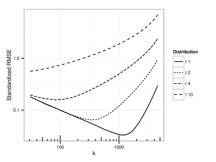
Figure 1: Estimated standardised rmse as a function of $k$ for samples of size $10000$ from Student’s distributions with different degrees of freedom $\nu=1,2,4,10$. All four distributions satisfy Condition (2.7) with $|\rho|=2/\nu$. The increasing parts of the lines reflect the values of $\rho$. rmse is estimated by averaging over $5000$ Monte-Carlo simulations.

Under this second-order condition (2.7), Hall and Welsh proved that the asymptotic mean squared error of the Hill estimator is minimal for sequences $(k_{n}^{*})_{n}$ satisfying

$$k^{*}_{n}\sim K(C,D,\rho)\,n^{2|\rho|/(1+2|\rho|)}$$

with $K(C,D,\rho)=\left({C^{2|\rho|}(1+|\rho|)^{2}}/{2D^{2}|\rho|^{3}}\right)^{1/(1+2|\rho|)}$. Since $C>0$, $D\neq 0$ and the second-order parameter $\rho<0$ are usually unknown, many authors have been interested in the construction of data-driven selection procedures for $k_{n}$ under conditions such as (2.7). A great deal of ingenuity has been dedicated to the estimation of the second-order parameters and to the use of such estimates when estimating first order parameters.

As we do not want to assume a second-order condition such as Condition (2.7), we resort to Lepski’s method which is a general attempt to balance bias and variance.

Since its introduction (Lepski, 1991), this general method for model selection has been proved to achieve adaptivity and to provide one with oracle inequalities in a variety of inferential contexts ranging from density estimation to inverse problems and classification (Lepski and Tsybakov, 2000; Lepski, 1991, 1990, 1992). Very readable introductions to Lepski’s method and its connections with penalised contrast methods can be found in (Birgé, 2001; Mathé, 2006). In EVT, we are aware of three papers that explicitly rely on this methodology: (Drees and Kaufmann, 1998), (Grama and Spokoiny, 2008) and (Carpentier and Kim, 2015).

The selection rule analysed in the present paper (see Section 3.2 for a precise definition) is a variant of the preliminary selection rule introduced in (Drees and Kaufmann, 1998)

$$\overline{\kappa}_{n}(r_{n})=\min\left\{k\in\{2,\ldots,n\}\colon\max_{2\leq i\leq k}\sqrt{i}|\widehat{\gamma}(i)-\widehat{\gamma}(k)|>r_{n}\right\}$$ (2.8)

where $(r_{n})_{n}$ is a sequence of thresholds such that $\sqrt{\ln\ln n}=o(r_{n})$ and $r_{n}=o(\sqrt{n})$, and $\widehat{\gamma}(i)$ is the Hill estimator computed from the $(i+1)$ largest order statistics. The definition of this “stopping time” is motivated by Lemma 1 from (Drees and Kaufmann, 1998) which asserts that, under the von Mises condition,

$$\max_{2\leq i\leq k_{n}}\sqrt{i}|\widehat{\gamma}(i)-\mathbb{E}\left[\widehat{\gamma}(i)\right]|=O_{P}\left(\sqrt{\ln\ln n}\right)\enspace.$$

In words, this selection rule almost picks out the largest index $k$ such that, for all $i$ smaller than $k$, $\widehat{\gamma}(k)$ differs from $\widehat{\gamma}(i)$ by a quantity that is not much larger than the typical fluctuations of $\widehat{\gamma}(i)$. This index selection rule can be performed graphically by interpreting an alternative Hill plot as shown on Figure 2 (see Drees et al., 2000; Resnick, 2007, for a discussion on the merits of alt-Hill plots).

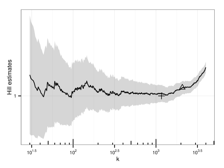
Figure 2: Lepski’s method illustrated on a alt-Hill plot. The plain line describes the sequence of Hill estimates as a function of index $k$ computed on a pseudo-random sample of size $n=10000$ from Student distribution with 1 degree of freedom (Cauchy distribution). Hill estimators are computed from the positive order statistics. The grey ribbon around the plain line provides a graphic illustration of Lepski’s method. For a given value of $i$, the width of the ribbon is $2r_{n}\widehat{\gamma}(i)/\sqrt{i}$. A point $(k,\widehat{\gamma}(k))$ on the plain line corresponds to an eligible index if the horizontal segment between this point and the vertical axis lies inside the ribbon that is, if for all $i,30\leq i<k$, $|\widehat{\gamma}(k)-\widehat{\gamma}(i)|\leq r_{n}\widehat{\gamma}(i)/\sqrt{i}$. If $r_{n}$ were replaced by an appropriate quantile of the Gaussian distribution, the grey ribbon would just represent the confidence tube that is usually added on Hill plots. The triangle represents the selected index with $r_{n}=\sqrt{2.1\ln\ln n}$. The cross represents the oracle index estimated from Monte-Carlo simulations, see Table 2.

The goal of Drees and Kaufmann (1998) is not to investigate the performance of the preliminary selection rule defined in Display (2.8) but to design a selection rule $\widehat{\kappa}_{n}(r_{n})$, based on $\overline{\kappa}_{n}(r_{n})$, that would asymptotically mimic the optimal selection rule $k^{*}_{n}$ under second-order conditions.

Our goal, as in (Grama and Spokoiny, 2008; Carpentier and Kim, 2015), is to derive non-asymptotic risk bounds without making a second-order assumption. In both papers, the rationale for working with some special collection of estimators seems to be the ability to derive non-asymptotic deviation inequalities for $\widehat{\gamma}(k)$ either from exponential inequalities for log-likelihood ratio statistics or from simple binomial tail inequalities such as Bernstein’s inequality (see Boucheron et al., 2013, Section 2.8).

In models satisfying Condition (2.7), the estimators from (Grama and Spokoiny, 2008) achieve the optimal rate up to a $\ln(n)$ factor. Carpentier and Kim (2015) prove that the risk of their data-driven estimator decays at the optimal rate $n^{|\rho|/(1+2|\rho|)}$ up to a factor $r_{n}^{2|\rho|/(1+2|\rho|)}=(\ln\ln n)^{|\rho|/(1+2|\rho|)}$ in models satisfying Condition (2.6).

We aim at achieving optimal risk bounds under Condition (2.6) using a simple estimation method requiring almost no calibration effort and based on mainstream extreme value index estimators. Before describing the keystone of our approach in Section 2.5, we recall the recent lower risk bound for adaptive extreme value index estimation.

2.4 Lower bound

One of the key results in (Carpentier and Kim, 2015) is a lower bound on the accuracy of adaptive tail index estimation. This lower bound reveals that, just as for estimating a density at a point (Lepski, 1991, 1992), or point estimation in Sobolev spaces (Tsybakov, 1998), as far as tail index estimation is concerned, adaptivity has a price. Using Fano’s Lemma, and a Bayesian game that extends cleanly in frameworks of (Grama and Spokoiny, 2008) and (Novak, 2014), Carpentier and Kim were able to prove the next minimax lower bound.

Theorem 2.9.

Let $\rho_{0}<-1$ and $v\in[0,\mathrm{e}/(1+2\mathrm{e})]$. Then, for any tail index estimator $\widehat{\gamma}$ and any sample size $n$ such that $M=\lfloor\ln n\rfloor>\mathrm{e}/v$, there exists a probability distribution $P$ such that

1. $P\in\mathsf{MDA}(\gamma)$ with $\gamma>0$,

2. $P$ meets the von Mises condition with von Mises function $\eta$ satisfying

   $$\overline{\eta}(t)\leq\gamma t^{\rho}$$

   for some $\rho\in[\rho_{0},0)$,

3. $$P\left\{|\widehat{\gamma}-\gamma|\geq\frac{C_{\rho}}{4}\gamma\left(\frac{v\ln\ln n}{n}\right)^{|\rho|/(1+2|\rho|)}\right\}\geq\frac{1}{1+2\mathrm{e}}$$

   and

   $$\mathbb{E}_{P}\left[\frac{|\widehat{\gamma}-\gamma|}{\gamma}\right]\geq\frac{C_{\rho}}{4(1+2\mathrm{e})}\left(\frac{v\ln\ln n}{n}\right)^{|\rho|/(1+2|\rho|)}\,,$$

   with $C_{\rho}=1-\exp\left(-\tfrac{1}{2(1+2|\rho|)^{2}}\right)$.

Using Birgé’s Lemma instead of Fano’s Lemma, we provide a simpler, shorter proof of this theorem (see Appendix E).

The lower rate of convergence provided by Theorem 2.9 is another incentive to revisit the preliminary tail index estimator from (Drees and Kaufmann, 1998). However, instead of using a sequence $(r_{n})_{n}$ of order larger than $\sqrt{\ln\ln n}$ in order to calibrate pairwise tests and ultimately to design estimators of the second-order parameter (if there are any), it is worth investigating a minimal sequence where $r_{n}$ is of order $\sqrt{\ln\ln n}$, and check whether the corresponding adaptive estimator achieves the Carpentier-Kim lower bound (Theorem 2.9).

In this paper, we focus on $r_{n}$ of the order $\sqrt{\ln\ln n}$. The rationale for imposing $r_{n}$ of the order $\sqrt{\ln\ln n}$ can be understood by the fact that, even if the sampling distribution is a pure Pareto distribution with shape parameter $\gamma$ ($\overline{F}(x)=(x/\tau)^{-1/\gamma}$ for $x\geq\tau>0$), if

$$\limsup r_{n}/(\gamma\sqrt{2\ln\ln n})<1\,,$$

the preliminary selection rule will, with high probability, select a small value of $k$ and thus pick out a suboptimal estimator. This can be justified using results from (Darling and Erdös, 1956) (see Appendix A for details).

Such an endeavour requires sharp probabilistic tools. They are the topic of the next section.

2.5 Talagrand’s concentration phenomenon for products of exponential distributions

Deriving authentic concentration inequalities for Hill estimators is not straightforward. Fortunately, the construction of such inequalities turns out to be possible thanks to general functional inequalities that hold for functions of independent exponentially distributed random variables. We recall these inequalities (Proposition 2.10 and Theorem 2.15) which have been largely overlooked in statistics. A thorough and readable presentation of these inequalities can be found in (Ledoux, 2001). We start by the easiest result, a variance bound that pertains to the family of Poincaré inequalities.

Proposition 2.10 (Poincaré inequality for exponentials, (Bobkov and Ledoux, 1997)).

If $g$ is a differentiable function over $\mathbb{R}^{n}$ and $Z=g(E_{1},\ldots,E_{n})$ where $E_{1},\ldots,E_{n}$ are independent standard exponential random variables, then

$$\operatorname{Var}(Z)\leq 4\mathbb{E}\left[\left\|\nabla g\right\|^{2}\right]\,.$$

Remark 2.11.

The constant $4$ can not be improved.

The next corollary is stated in order to point the relevance of this Poincaré inequality to the analysis of general order statistics and their functionals. Recall that the hazard rate of an absolutely continuous probability distribution with distribution $F$ is: $h=f/\overline{F}$ where $f$ and $\overline{F}=1-F$ are the density and the survival function associated with $F$, respectively.

Corollary 2.12.

Assume the distribution of $X$ has a positive density, then the $k$th order statistic $X_{(k)}$ satisfies

$$\operatorname{Var}(X_{(k)})\leq C\sum_{i=k}^{n}\frac{1}{i^{2}}\mathbb{E}\left[\frac{1}{h(X_{(k)})^{2}}\right]\leq\frac{C}{k}\left(1+\frac{1}{k}\right)\mathbb{E}\left[\frac{1}{h(X_{(k)})^{2}}\right]$$

where $C$ can be chosen as $4$.

Remark 2.13.

By Smirnov’s Lemma (de Haan and Ferreira, 2006), $C$ can not be smaller than $1$. If the distribution of $X$ has a non-decreasing hazard rate, the factor of $4$ can be improved into a factor $2$ (Boucheron and Thomas, 2012).

Talagrand (1991); Maurey (1991); Bobkov and Ledoux (1997) show that smooth functions of independent exponential random variables satisfy Bernstein type concentration inequalities. The next result is extracted from the derivation of Talagrand’s concentration phenomenon for product of exponential random variables in (Bobkov and Ledoux, 1997).

The definition of sub-gamma random variables will be used in the formulation of the theorem and in many arguments.

Definition 2.14.

A real-valued centred random variable $X$ is said to be sub-gamma on the right tail with variance factor $v$ and scale parameter $c$ if

$$\ln\mathbb{E}\mathrm{e}^{\lambda X}\leq\frac{\lambda^{2}v}{2(1-c\lambda)}\text{ for every }\lambda\quad\mbox{such that}\quad 0<\lambda<1/c\,.$$

We denote the collection of such random variables by $\Gamma_{+}(v,c)$. Similarly, $X$ is said to be sub-gamma on the left tail with variance factor $v$ and scale parameter $c$ if $-X$ is sub-gamma on the right tail with variance factor $v$ and tail parameter $c$. We denote the collection of such random variables by $\Gamma_{-}(v,c)$ and $\Gamma_{+}(v,c)\cap\Gamma_{-}(v,c)$ by $\Gamma_{\pm}(v,c)$.

If $X-\mathbb{E}X\in\Gamma_{+}(v,c)$, then for all $\delta\in(0,1)$, with probability larger than $1-\delta,$

$$X\leq\mathbb{E}X+\sqrt{2v\ln\left(1/\delta\right)}+c\ln\left(1/\delta\right)\,.$$

The entropy of a non-negative random variable $X$ is defined by $\operatorname{Ent}[X]=\mathbb{E}[X\ln X]-\mathbb{E}X\ln\mathbb{E}X$.

Theorem 2.15.

Assume that $g$ is a differentiable function on $\mathbb{R}^{n}$ with $\max_{i}|\partial_{i}g|<\infty$. Let $Z=g(E_{1},\ldots,E_{n})$ where $E_{1},\ldots,E_{n}$ are $n$ independent standard exponential random variables and $c<1$. Then, for all $\lambda$ such that $0\leq\lambda\max_{i}|\partial_{i}g|\leq c$,

$$\operatorname{Ent}\left[\mathrm{e}^{\lambda(Z-\mathbb{E}Z)}\right]\leq\frac{2\lambda^{2}}{1-c}\mathbb{E}\left[\mathrm{e}^{\lambda(Z-\mathbb{E}Z)}\|\nabla g\|^{2}\right]\,.$$

Let $v$ be the essential supremum of $\|\nabla g\|^{2}$, then $Z$ is sub-gamma on both tails with variance factor $4v$ and scale factor $\max_{i}|\partial_{i}g|$.

Again, we illustrate the relevance of these versatile tools on the analysis of general order statistics. This general theorem implies that if the sampling distribution has non-decreasing hazard rate, then the order statistics $X_{(k)}$ satisfy Bernstein type inequalities (see Boucheron et al., 2013, Section 2.8) with variance factor $4/k\mathbb{E}\left[{1}/{h(X_{(k)})^{2}}\right]$ (the Poincaré estimate of variance) and scale parameter $(\sup_{x}1/h(x))/k$). Starting back from the Efron-Stein-Steele inequality, the authors derived a somewhat sharper inequality (Boucheron and Thomas, 2012).

Corollary 2.16.

Assume the distribution function $F$ has non-decreasing hazard rate $h$ that is, $U\circ\ \exp$ is $C^{1}$ and concave. Let $Z=g(E_{1},\ldots,E_{n})=\left(U\circ\ \exp\right)\left(\sum_{i=k}^{n}E_{i}/i\right)$ be distributed as the $k$th order statistic of a sample distributed according to $F$. Then, $Z$ is sub-gamma on both tails with variance factor $4/k\left(1+1/k\right)\mathbb{E}[1/h(Z)^{2}]$ and scale factor $1/(k\inf_{x}h(x))$.

This corollary describes in which way central, intermediate and extreme order statistics can be portrayed as smooth functions of independent exponential random variables. This possibility should not be taken for granted as it is non trivial to capture in a non-asymptotic way the tail behaviour of maxima of independent Gaussians (Ledoux, 2001; Boucheron and Thomas, 2012; Chatterjee, 2014). In the next section, we show in which way the Hill estimator can fit into this picture.

3 Main results

In this section, the sampling distribution $F$ is assumed to belong to $\textsf{MDA}(\gamma)$ with $\gamma>0$ and to satisfy the von Mises condition (Definition 2.1) with bounded von Mises function $\eta$.

3.1 Variance and concentration inequalities for the Hill estimators

It is well known that, under the von Mises condition, if $(k_{n})$ is an intermediate sequence, the sequence $\sqrt{k_{n}}\left(\widehat{\gamma}(k_{n})-\mathbb{E}\widehat{\gamma}(k_{n})\right)$ converges in distribution towards $\mathcal{N}(0,\gamma^{2})$, suggesting that the variance of $\widehat{\gamma}(k_{n})$ scales like $\gamma^{2}/k_{n}$ (see Geluk et al., 1997; Beirlant et al., 2004; de Haan and Ferreira, 2006; Resnick, 2007).

Proposition 3.1 provides us with handy non-asymptotic bounds on $\operatorname{Var}[\widehat{\gamma}(k)]-\gamma^{2}/k$ using the von Mises function.

Proposition 3.1.

Let $\widehat{\gamma}(k)$ be the Hill estimator computed from the $(k+1)$ largest order statistics of an $n$-sample from $F$. Then,

$$-\frac{2\gamma}{k}\mathbb{E}\left[\overline{\eta}\left(\mathrm{e}^{Y_{(k+1)}}\right)\right]\leq\operatorname{Var}[\widehat{\gamma}(k)]-\frac{\gamma^{2}}{k}\leq\frac{2\gamma}{k}\mathbb{E}\left[\overline{\eta}\left(\mathrm{e}^{Y_{(k+1)}}\right)\right]+\frac{5}{k}\mathbb{E}\left[\overline{\eta}\left(\mathrm{e}^{Y_{(k+1)}}\right)^{2}\right]\,.$$

The next Abelian result might help in appreciating these variance bounds.

Proposition 3.2.

Assuming that $\eta$ is $\rho$-regularly varying with $\rho<0$, then, for any intermediate sequence $(k_{n})$,

$$\lim_{n\to\infty}\frac{k_{n}\operatorname{Var}(\widehat{\gamma}(k_{n}))-\gamma^{2}}{\eta(n/k_{n})}=\frac{2\gamma}{(1-\rho)^{2}}\,.$$

We may now move to genuine concentration inequalities for the Hill estimator.

The exponential representation (2.3) suggests that the rescaled Hill estimator $k\widehat{\gamma}(k)$ should be approximately distributed according to a $\text{gamma}(k,\gamma)$ distribution where $k$ is the shape parameter and $\gamma$ the scale parameter. Therefore, we expect the Hill estimators to satisfy Bernstein type concentration inequalities that is, to be sub-gamma on both tails with variance factors connected to the tail index $\gamma$ and to the von Mises function. Representation (2.3) actually suggests more. Following (Drees and Kaufmann, 1998), we actually expect the sequence $\big{(}\sqrt{k}(\widehat{\gamma}(k)-\mathbb{E}\widehat{\gamma}(k))\big{)}_{k}$ to behave like normalized partial sums of independent square integrable random variables that is, we believe $\max_{2\leq k\leq n}\sqrt{k}(\widehat{\gamma}(k)-\mathbb{E}\widehat{\gamma}(k))$ to scale like $\sqrt{\ln\ln n}$ and to be sub-gamma on both tails (see Appendix A). The purpose of this section is to meet these expectations in a non-asymptotic way.

Proofs use the Markov property of order statistics: conditionally on the $(J+1)$th order statistic, the first largest $J$ order statistics are distributed as the order statistics of a sample of size $J$ of the excess distribution. They consist of appropriate invocations of Talagrand’s concentration inequality (Theorem 2.15). However, this theorem generally requires a uniform bound on the gradient of the relevant function. When Hill estimators are analysed as functions of independent exponential random variables, the partial derivatives depend on the points at which the von Mises function is evaluated. In order to get interesting bounds, it is worth conditioning on an intermediate order statistic.

Throughout this subsection, let $\ell$ be an integer larger than $\sqrt{\ln n}$ and $J$ an integer not larger than $n$. We denote $E_{i},1\leq i\leq n$, $n$ independent standard exponential random variables and we work on the probability space where all $E_{i}$ are defined, and therefore consider the Hill estimators defined by Representation (2.3). As we use the exponential representation of order statistics, besides Hill estimators, the random variables that appear in the main statements are order statistics of exponential samples. As before, $Y_{(k)}$ will denote the $k$th order statistic of a standard exponential sample of size $n$ (we agree on $Y_{(n+1)}=0$).

The first theorem provides an exponential refinement of the variance bound stated in Proposition 3.1. However, as announced, there is a price to pay: statements hold conditionally on some order statistic. This is not an impediment to analyse Lepski’s rule using this theorem. Indeed, when analysing Lepki’s rule it is sufficient to control the Hill process $\left(\sqrt{i}(\widehat{\gamma}(i)-\mathbb{E}[\widehat{\gamma}(i)\mid Y_{(k+1)}])\right)_{i}$ for indices $i$ ranging between $\ell_{n}$ (that should not be smaller than $\ln(n)$) and some upper bound $k_{n}$ that achieves a certain balance between bias and standard deviation (the bias of $\widehat{\gamma}(k_{n})$ should be of order $r_{n}$ times the standard deviation, that is approximately $\gamma/\sqrt{k_{n}}$ where $r_{n}\approx\sqrt{\ln(\ln(n))}$). The second clause of next theorem is the cornerstone in the derivation of the risk bounds presented in the next section.

In the sequel, let

$$\xi_{n}=c_{1}\sqrt{\ln\log_{2}n}+c_{1}^{\prime},$$

where $c_{1}$ may be chosen not larger than $4$ and $c_{1}^{\prime}$ not larger than $34$.

Theorem 3.3.

Let $T$ be a shorthand for $\exp(Y_{(J+1)})$. For some $k$ such that $c_{2}\ln n\vee 32\leq\ell\leq k\leq J$ where $c_{2}\geq 2$, let

$$Z^{a}=\max_{\ell\leq i\leq k}\sqrt{i}\left|\widehat{\gamma}(i)-\mathbb{E}\left[\widehat{\gamma}(i)\mid Y_{(k+1)}\right]\right|\,.$$

Then, conditionally on $T$,

1. For $\ell\leq i\leq k$,

   $$\sqrt{i}\left(\widehat{\gamma}(i)-\mathbb{E}[\widehat{\gamma}(i)\mid T]\right)\in\Gamma_{\pm}\left(4\left(\gamma+3\overline{\eta}(T)\right)^{2},\left(\gamma+2\overline{\eta}(T)\right)\right)\,.$$

2. Let $u$ be such that $J\overline{\eta}(u)^{2}\leq\gamma^{2}r_{n}^{2}$ where $r_{n}=\sqrt{c_{3}\ln\ln n}$ with $c_{3}=2$. Assume that $T\geq u$, then

   $$Z^{a}\in\Gamma_{\pm}\left(4\gamma^{2}(1+3r_{n}/\sqrt{J})^{2},\gamma(1+2r_{n}/\sqrt{J})/\sqrt{\ell}\right)$$

   and

   $$\mathbb{E}\left[Z^{a}\mid T\right]\leq\gamma\xi_{n}\left(1+\frac{3r_{n}}{\sqrt{J}}\right)\,.$$

Remark 3.4.

If $F$ is a pure Pareto distribution with shape parameter $\gamma>0$, then $k\widehat{\gamma}(k)/\gamma$ is distributed according to a gamma distribution with shape parameter $k$ and scale parameter $1$. Tight and well-known tail bounds for gamma distributed random variables assert that

$$\mathbb{P}\left\{\left|\widehat{\gamma}(k)-\mathbb{E}\left[\widehat{\gamma}(k)\right]\right|\geq\frac{\gamma}{\sqrt{k}}\left(\sqrt{2\ln\left(2/\delta\right)}+\frac{\ln\left(2/\delta\right)}{\sqrt{k}}\right)\right\}\leq 2\delta\,.$$

Remark 3.5.

First part of Statement ii) reads as: conditionally on $\overline{\eta}(T)\leq r_{n}\gamma/\sqrt{J}$, with probability larger than $1-\delta$,

$$\left|Z^{a}-\mathbb{E}[Z^{a}\mid T]\right|\leq\gamma(1+3r_{n}/\sqrt{J})\left(\sqrt{8\ln\left(2/\delta\right)}+\frac{\ln\left(2/\delta\right)}{\sqrt{\ell}}\right)\,.\,$$

Combining both parts of Statement ii), we also get that, conditionally on $\overline{\eta}(T)\leq r_{n}\gamma/\sqrt{J}$, with probability larger than $1-\delta$,

$$Z^{a}\leq\gamma(1+3r_{n}/\sqrt{J})\left(\xi_{n}+\sqrt{8\ln\left(2/\delta\right)}+\frac{\ln\left(2/\delta\right)}{\sqrt{\ell}}\right)\,.$$

Remark 3.6.

The reader may wonder whether resorting to the exponential representation and usual Chernoff bounding would not provide a simpler argument. The straightforward approach leads to the following conditional bound on the logarithmic moment generating function,

$$\ln\mathbb{E}\left[\exp\left(\lambda\left(\widehat{\gamma}(k)-\mathbb{E}[\widehat{\gamma}(k)\mid Y_{(k+1)}]\right)\right)\mid Y_{(k+1)}\right]$$

$$\leq \frac{\left(\gamma+\overline{\eta}(\mathrm{e}^{Y_{(k+1)}})\right)^{2}}{2k\left(1-\lambda(\gamma+\overline{\eta}(\mathrm{e}^{Y_{(k+1)}}))\right)}+\lambda\left(\overline{\eta}(\mathrm{e}^{Y_{(k+1)}})-b\left(\mathrm{e}^{Y_{(k+1)}}\right)\right)\,.$$

A similar statement holds for the lower tail. This leads to exponential bounds for deviations of the Hill estimator above $\mathbb{E}[\widehat{\gamma}(k)\mid Y_{(k+1)}]+\overline{\eta}(\mathrm{e}^{Y_{(k+1)}})-b\left(\mathrm{e}^{Y_{(k+1)}}\right)$ that is, to control deviations of the Hill estimator above its expectation plus a term that may be of the order of magnitude of the bias.

Attempts to rewrite $\widehat{\gamma}(k)-\mathbb{E}[\widehat{\gamma}(k)\mid Y_{(k+1)}]$ as a sum of martingale increments $\mathbb{E}[\widehat{\gamma}(k)\mid Y_{(i)}]-\mathbb{E}[\widehat{\gamma}(k)\mid Y_{(i+1)}]$, for $1\leq i\leq k$, and to exhibit an exponential supermartingale met the same impediments.

At the expense of inflating the variance factor, Theorem 2.15 provides a genuine (conditional) concentration inequality for Hill estimators. As we will deal with values of $k$ for which bias exceeds the typical order of magnitudes of fluctuations, this is relevant to our purpose.

3.2 Adaptive Hill estimation

We are now able to characterise the performance of the variant of the selection rule defined by (2.8) (Drees and Kaufmann, 1998) with $r_{n}=\sqrt{c_{3}\ln\ln n}$ where $c_{3}=2$. Let $\ell_{n}=\lceil c_{2}\ln n\rceil$ where $c_{2}$ is a constant to be defined below.

The deterministic sequence of indices $(k_{n}(r_{n}))$ is defined (for $n$ large enough) by

$$k_{n}(r_{n})=\max\left\{k\in\{\ell_{n},\ldots,n\}\colon\sqrt{k}\overline{\eta}(n/k^{\delta})\leq\gamma r_{n}\right\}\,,$$ (3.7)

where $k^{\delta}=k+\sqrt{2k\ln(1/\delta)}+2\ln(1/\delta).$ The sequence $(k_{n}(1))_{n}$ is defined by choosing $r_{n}=1$. The deterministic sequences $(k_{n}(1))$ and $(k_{n}(r_{n}))$ achieve specific balances between bias and variance. In full generality, because $\overline{\eta}(t)$ is just an upper bound on the conditional bias $b(t)$, it is difficult to precisely connect $(k_{n}(1))$ and $(k_{n}(r_{n}))$ with the oracle sequence $(k^{*}_{n})$. We call these two sequences the pivotal sequences. In the sequel, $k_{n}$ stands for $k_{n}(r_{n})$. If the context is not clear, we specify $k_{n}(1)$ or $\ k_{n}(r_{n})$.

Let $1/(2n)<\delta<1/4$. Recall, from Section 3.1, that $\xi_{n}=c_{1}\sqrt{\ln\ln(n)}+c^{\prime}_{1}$ and agree on the shorthands

$$z_{\delta} =(1+3r_{n}/\sqrt{k_{n}})\left(\xi_{n}+\sqrt{8\ln\left(2/\delta\right)}+\frac{\ln\left(2/\delta\right)}{\sqrt{\ell_{n}}}\right)$$

and $\overline{z}_{\delta}$ which is defined by replacing $k_{n}$ by $\ell_{n}$ in the definition of $z_{\delta}$ ($\overline{z}_{\delta}$ depends on $n,\delta$ but not on the sampling distribution). In the sequel, $c_{2}$ is assumed to be chosen so that $r_{n}+\overline{z}_{\delta}\leq 9\sqrt{c_{2}\ln(n)}/10$ for $n>1000$ and $2/n<\delta<1/4$ ($c_{2}$ may be chosen not larger than 100).

The index $\widehat{k}_{n}$ is selected according to the following rule:

$$\widehat{k}_{n}=\max\left\{k\in\{\ell_{n},\ldots,n\}\text{ and }\forall i\in\{\ell_{n},\ldots,n\}\,,\left|\widehat{\gamma}(i)-\widehat{\gamma}(k)\right|\leq\frac{\widehat{\gamma}(i)r_{n}(\delta)}{\sqrt{i}}\right\}$$

where $r_{n}(\delta)=10(r_{n}+\overline{z}_{\delta})$. The quantity $r_{n}(\delta)$ scales like $\sqrt{\ln((2/\delta)\ln(n))}$. The tail index estimator is $\widehat{\gamma}(\widehat{k}_{n})$.

As tail adaptivity has a price (see Theorem  2.9), the ratio between the risk of the data-driven estimator $\widehat{\gamma}(\widehat{k}_{n})$ and the risk of the pivotal index $\widehat{\gamma}(k_{n}(1))$ cannot be upper bounded by a constant factor, let alone by a factor close to $1$. This is why in the next theorem, we compare the risk of the empirically selected index $\widehat{\gamma}(\widehat{k}_{n})$ with the risk of the pivotal index $\widehat{\gamma}(k_{n})$.

Recall, from Section 3.1, that

$$\xi_{n}=c_{1}\sqrt{\ln\log_{2}n}+c^{\prime}_{1}\quad\text{with }c_{1}\leq 4\text{ and }c^{\prime}_{1}\leq 34\,.$$

Theorem 3.8.

Assume the sampling distribution $F\in\mathsf{MDA}(\gamma),\gamma>0$ satisfies the von Mises condition with bounded von Mises function $\eta$, and $\overline{\eta}(t)=\sup_{s\geq t}|\eta(s)|.$

Let $n>1000$ is large enough so that $k_{n}$ (Definition 3.7) is well defined. Then, for $2/n<\delta<1/4$, with probability larger than $1-3\delta$,

$$\Big{|}\gamma-\widehat{\gamma}(\widehat{k}_{n})\Big{|}\leq\left|\gamma-\widehat{\gamma}(k_{n})\right|\left(1+\tfrac{r_{n}(\delta)}{\sqrt{k_{n}}}\right)+\tfrac{r_{n}(\delta)}{\sqrt{k_{n}}}\gamma\,,$$

and, with probability larger than $1-4\delta$,

$$\Big{|}\widehat{\gamma}(\widehat{k}_{n})-\gamma\Big{|} \leq \tfrac{2r_{n}(\delta)}{\sqrt{k_{n}}}\gamma\left(1+\alpha(\delta,n)\right)\,,$$ (3.9)

where

$$\alpha(\delta,n) \leq \frac{r_{n}}{2\sqrt{\ell_{n}}}+\frac{\sqrt{\ln(2/\delta)}}{r_{n}(\delta)}\left(1+\frac{3r_{n}(\delta)}{\sqrt{\ell_{n}}}\right)^{2}\,.$$

Remark 3.10.

For $0<\delta<1/2$,

$$\alpha(\delta,n)=o(1)\quad\text{as $n\to\infty$}\enspace.$$

Remark 3.11.

If the bias $b$ is $\rho$-regularly varying (or equivalently, if the von Mises function $\eta$ or even $\overline{\eta}$ are regularly varying), then, elaborating on Proposition 1 from (Drees and Kaufmann, 1998), sequences $(k_{n}^{*})$ and $(k_{n}(1))$ are connected by

$$\lim_{n}\frac{k_{n}(1)}{k_{n}^{*}}=(2|\rho|)^{1/(1+2|\rho|)}$$

and their quadratic risk are related by

$$\lim_{n}\frac{\mathbb{E}[(\gamma-\widehat{\gamma}(k_{n}(1)))^{2}]}{\mathbb{E}[(\gamma-\widehat{\gamma}(k_{n}^{*}))^{2}]}=\frac{2}{2|\rho|+1}(2|\rho|)^{2|\rho|/(1+2|\rho|)}\,.$$

Moreover, under the second-order assumption, the two pivotal sequences $(k_{n}(1))$ and $(k_{n}(r_{n}))$ are also connected.

Thus, if the bias is $\rho$-regularly varying, Theorem 3.8 provides us with a connection between the performance of the simple selection rule and the performance of the (asymptotically) optimal choice.

Recall that one of the main aims of this paper is to derive performance guarantees for the data-driven index selection method $\widehat{k}_{n}$ without resorting to second-order assumptions that is, without assuming that the von Mises function is regularly varying. The next corollary upper bounds the risk of the preliminary estimator when we just have an upper bound on the bias.

Corollary 3.12.

Assume that, for some $C>0$ and $\rho<0$, for all $t>1$,

$$\overline{\eta}\left(t\right)\leq Ct^{\rho}\,.$$

Then, there exists a constant $\kappa_{C,\delta,\rho}$ depending on $C,\delta$ and $\rho$ such that, with probability larger than $1-4\delta$,

$$\Big{|}\widehat{\gamma}(\widehat{k}_{n})-\gamma\Big{|} \leq \kappa_{C,\delta,\rho}\left(\frac{\gamma^{2}\ln\left((2/\delta)\ln n\right)}{n}\right)^{|\rho|/(1+2|\rho|)}\left(1+\alpha(\delta,n)\right)$$

where $\alpha(\delta,n)$ is defined in Theorem 3.8.

This meets the information-theoretic lower bound of Theorem 2.9.

4 Proofs

4.1 Proof of Proposition 2.2

This proposition is a straightforward consequence of Rényi’s representation of order statistics of standard exponential samples.

As $F$ belongs to $\textsf{MDA}(\gamma)$ and meets the von Mises condition, there exists a function $\eta$ on $(1,\infty)$ with $\lim_{x\to\infty}\eta(x)=0$ such that

$$U(x)=cx^{\gamma}\exp\left(\int_{1}^{x}\frac{\eta(s)}{s}\mathrm{d}s\right)\,,$$

and

$$U(\mathrm{e}^{y})=c\exp\left(\int_{0}^{y}(\gamma+\eta(\mathrm{e}^{u}))\mathrm{d}u\right)\,.$$

Then,

$$\widehat{\gamma}(k) \stackrel{{\scriptstyle d}}{{=}} \frac{1}{k}\sum_{i=1}^{k}i\frac{\ln U\left(\mathrm{e}^{Y_{(i)}}\right)}{\ln U\left(\mathrm{e}^{Y_{(i+1)}}\right)}$$

$$\stackrel{{\scriptstyle d}}{{=}} \frac{1}{k}\sum_{i=1}^{k}i\int_{Y_{(i+1)}}^{Y_{(i)}}(\gamma+\eta(\mathrm{e}^{u}))\mathrm{d}u$$

$$\stackrel{{\scriptstyle d}}{{=}} \frac{1}{k}\sum_{i=1}^{k}i\int_{0}^{E_{i}/i}(\gamma+\eta(\mathrm{e}^{u+Y_{(i+1)}}))\mathrm{d}u$$

$$\stackrel{{\scriptstyle d}}{{=}} \frac{1}{k}\sum_{i=1}^{k}\int_{0}^{E_{i}}(\gamma+\eta(\mathrm{e}^{\tfrac{u}{i}+Y_{(i+1)}}))\mathrm{d}u\,.$$

4.2 Proof of Proposition 3.1

Let $Z=k\widehat{\gamma}(k)$. By the Pythagorean relation,

$$\operatorname{Var}(Z)=\mathbb{E}\left[\operatorname{Var}\left(Z\mid Y_{(k+1)}\right)\right]+\operatorname{Var}\left(\mathbb{E}[Z\mid Y_{(k+1)}]\right)\,.$$

Representation (2.4) asserts that, conditionally on $Y_{(k+1)}$, $Z$ is distributed as a sum of independent, exponentially distributed random variables. Let $E$ be an exponentially distributed random variable.

$$\operatorname{Var}\left(Z\mid Y_{(k+1)}=y\right)$$

$$= k\operatorname{Var}\biggl{(}\gamma E+\int_{0}^{E}\eta(\mathrm{e}^{u+y})\mathrm{d}u\biggr{)}$$

$$= k\gamma^{2}+2k\gamma\operatorname{Cov}\biggl{(}E,\int_{0}^{E}\eta(\mathrm{e}^{u+y})\mathrm{d}u\biggr{)}+\operatorname{Var}\biggl{(}\int_{0}^{E}\eta(\mathrm{e}^{u+y})\mathrm{d}u\biggl{)}$$

$$\leq k\gamma^{2}+2k\gamma\overline{\eta}(\mathrm{e}^{y})+k\left(\overline{\eta}\left(\mathrm{e}^{y}\right)\right)^{2}\,,$$

where we have used the Cauchy-Schwarz inequality and $\operatorname{Var}\bigl{(}\int_{0}^{E}\eta(\mathrm{e}^{y+u})\mathrm{d}u\bigl{)}\leq\overline{\eta}(\mathrm{e}^{y})^{2}.$ Taking expectation with respect to $Y_{(k+1)}$ leads to

$$\mathbb{E}\left[\operatorname{Var}\left(Z\mid Y_{(k+1)}\right)\right]\leq k{\gamma^{2}}+2k\gamma\mathbb{E}\left[\overline{\eta}\left(\mathrm{e}^{Y_{(k+1)}}\right)\right]+k{\mathbb{E}\left[\overline{\eta}\left(\mathrm{e}^{Y_{(k+1)}}\right)^{2}\right]}\,.$$

The last term in the Pythagorean decomposition is also handled using elementary arguments.

$$\mathbb{E}[Z\mid Y_{(k+1)}]=k\gamma+k\int_{0}^{\infty}\mathrm{e}^{-u}\eta\left(\mathrm{e}^{u+Y_{(k+1)}}\right)\mathrm{d}u\,.$$

As $Y_{(k+1)}$ is a function of independent exponential random variables ($Y_{(k+1)}=\sum_{i=k+1}^{n}E_{i}/i$), the variance of $\mathbb{E}[Z\mid Y_{(k+1)}]$ may be upper bounded using Poincaré inequality (Proposition 2.10)

$$\operatorname{Var}\left(\mathbb{E}[Z\mid Y_{(k+1)}]\right)\leq 4k\mathbb{E}\left[\overline{\eta}\left(\mathrm{e}^{Y_{(k+1)}}\right)^{2}\right]\,.$$

In order to derive the lower bound, we first observe that

$$\operatorname{Var}(Z)\geq\mathbb{E}\left[\operatorname{Var}\left(Z\mid Y_{(k+1)}\right)\right]\,.$$

Now, using Cauchy-Schwarz inequality again,

$$\operatorname{Var}\left(Z\mid Y_{(k+1)}=y\right) \geq k\gamma^{2}-2k\gamma\bigg{\lvert}\operatorname{Cov}\bigl{(}E,\int_{0}^{E}\eta(\mathrm{e}^{u+y})\mathrm{d}u\bigr{)}\bigg{\rvert}$$

$$\geq k\gamma^{2}-2k\gamma\bigg{(}\operatorname{Var}\bigg{(}\int_{0}^{E}\eta(\mathrm{e}^{u+y})\mathrm{d}u\bigg{)}\bigg{)}^{1/2}$$

$$\geq k\gamma^{2}-2k\gamma\overline{\eta}(\mathrm{e}^{y})\,.$$

4.3 Proof of Theorem 3.3

In the proof of Theorem 3.3, we will use the next maximal inequality (see Boucheron et al., 2013, Corollary 2.6). Recall the definition of $\Gamma_{+}(v,c)$ (Definition 2.14).

Proposition 4.1.

Let $Z_{1},\ldots,Z_{N}$ be real-valued random variables belonging to $\Gamma_{+}(v,c)$. Then

$$\mathbb{E}\left[\max_{i=1,\ldots,N}Z_{i}\right]\leq\sqrt{2v\ln N}+c\ln N~{}.$$

Proofs follow a common pattern. In order to check that some random variable is sub-gamma, we rely on its representation as a function of independent exponential variables and compute partial derivatives, derive convenient upper bounds on the squared Euclidean norm and the supremum norm of the gradient and then invoke Theorem 2.15.

At some point, we will use the next corollary of Theorem 2.15.

Corollary 4.2.

If $g$ is an almost everywhere differentiable function on $\mathbb{R}$ with uniformly bounded derivative $g^{\prime}$, then $g(Y_{(k+1)})$ is sub-gamma with variance factor $4\|g^{\prime}\|^{2}_{\infty}/k$ and scale factor $\|g^{\prime}\|_{\infty}/k.$

Proof of Theorem 3.3.

We start from the exponential representation of Hill estimators (Proposition 2.2) and represent all $\widehat{\gamma}(i)$ as functions of independent random variables $E_{1},\ldots,E_{{k}},\ldots,E_{J},Y_{({J+1})}$ where the $E_{j},1\leq j\leq J$, are standard exponentially distributed and $Y_{({J+1})}$ is distributed like the $(J+1)$th largest order statistic of an $n$-sample of the standard exponential distribution. We consistently use the notation $Y_{(k)}=\sum_{j=k}^{J}\frac{E_{j}}{j}+Y_{(J+1)}$, for $1\leq k\leq J$.

$$i\widehat{\gamma}(i) = \sum_{j=1}^{i}\int_{0}^{E_{j}}\left(\gamma+\eta(\mathrm{e}^{\frac{u}{j}+Y_{({j+1})}})\right)\mathrm{d}u$$

$$= \sum_{j=1}^{i}\left(\gamma E_{j}+j\int_{Y_{(j+1)}}^{Y_{(j)}}\eta(\mathrm{e}^{v})\,\mathrm{d}v\right)\,.$$

Let $i^{\prime}$ be such that $0\leq i^{\prime}<i$, let us agree on $\widehat{\gamma}(0)=0.$ Let

$$g(E_{i^{\prime}+1},\dots,E_{J}) = i\widehat{\gamma}(i)-i^{\prime}\widehat{\gamma}(i^{\prime})$$

$$= \sum_{j=i^{\prime}+1}^{i}\gamma E_{j}+\sum_{j=i^{\prime}+1}^{i}j\int_{Y_{(j+1)}}^{Y_{(j)}}\eta(\mathrm{e}^{v})\,\mathrm{d}v\,.$$

For $i^{\prime}<p\leq i$, as $\frac{\partial Y_{(j)}}{\partial x_{p}}=\frac{1}{p}$ for $j\leq p$ and $0$ otherwise,

$$\frac{\partial g}{\partial x_{p}} = \gamma+\sum_{j=i^{\prime}+1}^{p}j\frac{\partial\int_{Y_{(j+1)}}^{Y_{(j)}}\eta(\mathrm{e}^{v})\mathrm{d}v}{\partial x_{p}}$$

$$= \gamma+\eta(\mathrm{e}^{Y_{(p)}})+\sum_{j=i^{\prime}+1}^{p-1}\frac{j}{p}\left(\eta(\mathrm{e}^{Y_{(j)}})-\eta(\mathrm{e}^{Y_{(j+1)}})\right)$$

$$= \gamma+\sum_{j=i^{\prime}+2}^{p}\frac{\eta(\mathrm{e}^{Y_{(j)}})}{p}+\frac{(i^{\prime}+1)\eta(\mathrm{e}^{Y_{(i^{\prime}+1)}})}{p}\,.$$

This entails that, for $i^{\prime}<p\leq i$,

$$\left|{\frac{\partial g}{\partial x_{p}}}\right|\leq\gamma+\sum_{j=1}^{p}\frac{\overline{\eta}(\mathrm{e}^{Y_{(p\vee i^{\prime}+1)}})}{p}\leq\gamma+\overline{\eta}(\mathrm{e}^{Y_{(p)}})\,.$$ (4.3)

For $i<p\leq J$,

$$\frac{\partial g}{\partial x_{p}} = \sum_{j=i^{\prime}+1}^{i}j\frac{\partial\int_{Y_{(j+1)}}^{Y_{(j)}}\eta(\mathrm{e}^{v})\,\mathrm{d}v}{\partial x_{p}}$$

$$= \sum_{j=i^{\prime}+1}^{i}\frac{j}{p}\left(\eta(\mathrm{e}^{Y_{(j)}})-\eta(\mathrm{e}^{Y_{(j+1)}})\right)$$

$$= \frac{1}{p}\left(\sum_{j=i^{\prime}+2}^{i}\eta(\mathrm{e}^{Y_{(j)}})+(i^{\prime}+1)\eta(\mathrm{e}^{Y_{(i^{\prime}+1)}})-i\eta(\mathrm{e}^{Y_{(i+1)}})\right)$$

$$= \frac{1}{p}\left(\sum_{j=i^{\prime}+1}^{i}\left(\eta(\mathrm{e}^{Y_{(j)}})-\eta(\mathrm{e}^{Y_{(i+1)}})\right)+i^{\prime}\left(\eta(\mathrm{e}^{Y_{(i^{\prime}+1)}})-\eta(\mathrm{e}^{Y_{(i+1)}})\right)\right)\,.$$

This is enough to entail that, for $i<p\leq k$,

$$\left|{\frac{\partial g}{\partial x_{p}}}\right|\leq\frac{2i}{p}\overline{\eta}(\mathrm{e}^{Y_{(p)}})\,.$$ (4.4)

All in all, for $1\leq p\leq k$,

$$\left|{\frac{\partial g}{\partial x_{p}}}\right|\leq(\gamma+\overline{\eta}(T))\vee 2\overline{\eta}(T)\leq\gamma+2\overline{\eta}(T)\,.$$

Proof of i)

An upper bound on the variance factor for $i\widehat{\gamma}(i)$, conditionally on $T$, is obtained by specialising to the case $i^{\prime}=0$ and using (4.3) and (4.4) as well as the monotonicity of $\overline{\eta}$,

$$\sum_{p=1}^{J}\left|\frac{\partial g}{\partial x_{p}}\right|^{2} \leq \sum_{p=1}^{i}\left(\gamma+\overline{\eta}(\mathrm{e}^{Y_{(p)}})\right)^{2}+\sum_{p=i+1}^{J}\frac{4i^{2}}{p^{2}}\overline{\eta}(\mathrm{e}^{Y_{(p)}})^{2}$$

$$\leq {i}\left(\left(\gamma+\overline{\eta}(T)\right)^{2}+4\left(\overline{\eta}(T)\right)^{2}\right)\leq i\left(\gamma+3\overline{\eta}(T)\right)^{2}\,.$$

Using Theorem 2.15 conditionally on $T=\exp(Y_{(J+1)})$, we realise that $\sqrt{i}(\widehat{\gamma}(i)-\mathbb{E}\left[\widehat{\gamma}(i)\mid T\right])$ is sub-gamma on both sides with variance factor not larger than $4\left(\gamma+3\overline{\eta}(T)\right)^{2}$ and scale factor not larger than $\gamma+2\overline{\eta}(T)$. This yields

$$\mathbb{P} \left\{\lvert\widehat{\gamma}(i)-\mathbb{E}\left[\widehat{\gamma}(i)\mid T\right]\rvert\geq\frac{\gamma+3\overline{\eta}\left(T\right)}{\sqrt{i}}\left(\sqrt{8s}+\frac{s}{\sqrt{i}}\right)\mid T\right\}\leq 2\mathrm{e}^{-s}\,.$$

Taking expectation on both sides, this implies that

$$\mathbb{P} \left\{\lvert\widehat{\gamma}(i)-\mathbb{E}\left[\widehat{\gamma}(i)\mid T\right]\rvert\geq\frac{\gamma+3\overline{\eta}\left(T\right)}{\sqrt{i}}\left(\sqrt{8s}+\frac{s}{\sqrt{i}}\right)\right\}\leq 2\mathrm{e}^{-s}\,.$$

Proof of ii)

The proof of the upper bound on $\mathbb{E}[Z^{a}\mid T]$ in Statement ii) from Theorem 3.3 relies on standard chaining techniques from the theory of empirical processes and uses repeatedly the concentration Theorem 2.15 for smooth functions of independent exponential random variables and the maximal inequality for sub-gamma random variables (Proposition 4.1).

For general $i^{\prime}$, the variance factor for $i\widehat{\gamma}(i)-i^{\prime}\widehat{\gamma}(i^{\prime})$ is upper bounded by

$$(i-i^{\prime})\left(\gamma+\overline{\eta}(T)\right)^{2}+\sum_{p=i+1}^{J}\frac{i^{2}}{p^{2}}\left(2\overline{\eta}(T)\right)^{2}\leq(i-i^{\prime})\left(\gamma+\overline{\eta}(T)\right)^{2}+i(2\overline{\eta}(T))^{2}\,.$$

Let $u$ be such that $J\overline{\eta}(u)^{2}\leq\gamma^{2}r_{n}^{2}$ where $r_{n}=\sqrt{c_{3}\ln\ln n}$ with $c_{3}=2$. Now, as we assume, in the sequel, that $T>u$, we may use the next upper bound for the variance factor of $i\widehat{\gamma}(i)-i^{\prime}\widehat{\gamma}(i^{\prime})$ (conditionally on $Y_{(J+1)}$),

$$4\gamma^{2}\left((i-i^{\prime})\Big{(}1+\frac{r_{n}}{\sqrt{J}}\Big{)}^{2}+4r_{n}^{2}\right)\,.$$

Recall that

$$Z^{a}=\max_{\ell\leq i\leq k}\sqrt{i}\left|\widehat{\gamma}(i)-\mathbb{E}\left[\widehat{\gamma}(i)\mid Y_{(k+1)}\right]\right|\,.$$

As it is commonplace in the analysis of normalised empirical processes (see van de Geer, 2000; Giné and Koltchinskii, 2006; Massart, 2007, and references therein), we peel the index set over which the maximum is computed.

Let $\mathcal{L}_{n}=\{\lfloor\log_{2}(\ell)\rfloor,\ldots,\lfloor\log_{2}({k})\rfloor\}$ and, for all $j \in\mathcal{L}_{n}$, $\mathcal{S}_{j}=\{\ell\vee 2^{j},\ldots,k\wedge 2^{j+1}-1\}$. Define $Z^{a}_{j}$ as

$$Z^{a}_{j}=\max_{i\in\mathcal{S}_{j}}\sqrt{i}\left|\widehat{\gamma}(i)-\mathbb{E}\left[\widehat{\gamma}(i)\mid Y_{(k+1)}\right]\right|\,.$$

Then,

$$\mathbb{E}[Z^{a}\mid Y_{(k+1)}] = \mathbb{E}[\max_{j\in\mathcal{L}_{n}}Z^{a}_{j}\mid Y_{(k+1)}]$$

$$\leq \mathbb{E}[\max_{j\in\mathcal{L}_{n}}(Z^{a}_{j}-\mathbb{E}[Z^{a}_{j}\mid Y_{(k+1)}])\mid Y_{(k+1)}]]+\max_{j\in\mathcal{L}_{n}}\mathbb{E}[Z^{a}_{j}\mid Y_{(k+1)}]]\,.$$

We now derive upper bounds on both summands by resorting to the maximum inequality for sub-gamma random variables (Proposition 4.1). We first bound $\mathbb{E}[Z^{a}_{j}\mid Y_{(k+1)}]$, for $j\in\mathcal{L}_{n}$.

Note that direct invocation of Lemma 4.1 and Statement i) shows that

$$\mathbb{E}[Z^{a}_{j}\mid Y_{(k+1)}]\leq 2\gamma(1+3r/\sqrt{J})\left(\sqrt{8j\ln(2)}+j\ln(2)\right)\,.$$ (4.5)

This bound will be useful for handling small values of $j$. For $j\leq 11$, $\sqrt{8j\ln(2)}+j\ln(2)\leq 16$.

We now handle generic $j$ using chaining. Fix $j\in\mathcal{L}_{n}$,

$$\max_{i\in\mathcal{S}_{j}}\sqrt{i}\left|\widehat{\gamma}(i)-\mathbb{E}[\widehat{\gamma}(i)\mid Y_{(k+1)}]\right|\leq\frac{1}{2^{j/2}}\max_{i\in\mathcal{S}_{j}}\,i\left|\widehat{\gamma}(i)-\mathbb{E}[\widehat{\gamma}(i)\mid Y_{(k+1)}]\right|\,.$$

In order to alleviate notation, let $W(i)=i\left(\widehat{\gamma}({i})-\mathbb{E}[\widehat{\gamma}({i})\mid Y_{(k+1)}]\right)$, for $i\in\mathcal{S}_{j}$. For $i\in\mathcal{S}_{j}$, let

$$i=2^{j}+\sum_{m=1}^{j}b_{m}2^{j-m}\ \text{ where $b_{m}\in\{0,1\}$}$$

be the binary expansion of $i$. Then, for $h\in\{0,\ldots,j\}$, let $\pi_{h}(i)$ be defined by

$$\pi_{h}(i)=2^{j}+\sum_{m=1}^{h}b_{m}2^{j-m}\,$$

so that $\pi_{j}(i)=i$, $\pi_{0}(i)=2^{j}$ and $0\leq\pi_{h+1}(i)-\pi_{h}(i)\leq 2^{j-h-1}$.

Using the fact that $W(\pi_{0}(i))$ does not depend on $i$ and that

$$\mathbb{E}\left[W(\pi_{0}(i))\mid Y_{(k+1)}\right]=0\,,$$

we obtain

$$\mathbb{E}\left[\max_{i\in\mathcal{S}_{j}}i\left(\widehat{\gamma}(i)-\mathbb{E}\left[\widehat{\gamma}(i)\mid Y_{(k+1)}\right]\right)\mid Y_{(k+1)}\right]$$

$$= \mathbb{E}\left[\max_{i\in\mathcal{S}_{j}}W(i)\mid Y_{(k+1)}\right]$$

$$= \mathbb{E}\left[\max_{i\in\mathcal{S}_{j}}W(\pi_{j}(i))-W(\pi_{0}(i))\mid Y_{(k+1)}\right]$$

$$= \mathbb{E}\left[\max_{i\in\mathcal{S}_{j}}\sum_{h=0}^{j-1}(W(\pi_{h+1}(i))-W(\pi_{h}(i)))\mid Y_{(k+1)}\right]$$

$$\leq \sum_{h=0}^{j-1}\mathbb{E}\left[\max_{i\in\mathcal{S}_{j}}(W(\pi_{h+1}(i))-W(\pi_{h}(i)))\mid Y_{(k+1)}\right]\,.$$

Now, for each $h\in\{0,\ldots,j-1\}$, the maximum is taken over $2^{h}$ random variables which are sub-gamma with variance factor

$$4\gamma^{2}\times\left(2^{j-h-1}\Big{(}1+\frac{r_{n}}{\sqrt{J}}\Big{)}^{2}+4r_{n}^{2}\right)$$

and scale factor $(\gamma+2\overline{\eta}(T))\leq\gamma(1+2r_{n}/\sqrt{J})$. By Proposition 4.1, since $i\in\mathcal{S}_{j}$,

$$\mathbb{E}\left[\max_{i\in\mathcal{S}_{j}}i\left(\widehat{\gamma}(i)-\mathbb{E}\left[\widehat{\gamma}(i)\mid Y_{(k+1)}\right]\right)\mid Y_{(k+1)}\right]$$

$$\leq \gamma\sum_{h=0}^{j-1}\left(\left(1+\frac{r_{n}}{\sqrt{J}}\right)\sqrt{8h2^{(j-h-1)}\ln 2}+\sqrt{32h\ln 2}r_{n}+\left(1+\frac{2r_{n}}{\sqrt{J}}\right)h\ln 2\right)$$

$$\leq \gamma\left(1+\frac{2r_{n}}{\sqrt{J}}\right)\left(2^{(j-1)/2}4.15\sqrt{8\ln 2}+\frac{2}{3}\sqrt{32c_{2}}\ln(2)j^{2}+\frac{j(j-1)}{2}\ln 2\right)$$

where we have used

$$4.15 \geq \sum_{h=0}^{\infty}\sqrt{h2^{-h}}$$

$$r_{n} \leq \sqrt{c_{2}\ln(2)}j^{1/2}\text{ as }r_{n}=\sqrt{c_{3}\ln\ln(n)},j+1\geq\log_{2}(c_{2}\ln(n))\,.$$

For $j\geq 12$,

$${\mathbb{E}\left[\max_{i\in\mathcal{S}_{j}}i\left(\widehat{\gamma}(i)-\mathbb{E}\left[\widehat{\gamma}(i)\mid Y_{(k+1)}\right]\right)\mid Y_{(k+1)}\right]} \leq 17\gamma\,2^{j/2}\left(1+\frac{2r_{n}}{\sqrt{J}}\right)\,.$$

Finally, for all $j\in\mathcal{L}_{n}$,

$$\mathbb{E}[Z^{a}_{j}\mid Y_{(k+1)}]\leq 34\,\gamma\,\left(1+\frac{3r_{n}}{\sqrt{J}}\right)\,.$$

In order to prove Statement ii), we check that, for each $j\in\mathcal{L}_{n}$, $Z^{a}_{j}$ is sub-gamma on the right-tail with variance factor at most $4\left(\gamma+3\overline{\eta}(T)\right)^{2}$ and scale factor not larger than $\left(\gamma+3\overline{\eta}(T)\right)/\sqrt{\ell}$. Under the von Mises condition (Definition 2.1), the sampling distribution is absolutely continuous with respect to Lebesgue measure. For almost every sample, the maximum defining $Z^{a}_{j}$ is attained at a single index $i\in\mathcal{S}_{j}$. Starting again from the exponential representation and repeating the computation of partial derivatives, we obtain the desired bounds.

By Proposition 4.1,

$$\mathbb{E}\left[\max_{j\in\mathcal{L}_{n}}(Z^{a}_{j}-\mathbb{E}[Z^{a}_{j}\mid Y_{(k+1)}])\mid Y_{(k+1)}\right]$$

$$\leq \left(\sqrt{8\ln|\mathcal{L}_{n}|}+\frac{\ln|\mathcal{L}_{n}|}{\sqrt{\ell}}\right)\left(\gamma+3\overline{\eta}(T)\right)$$

$$\leq 4\sqrt{\ln|\mathcal{L}_{n}|}\left(\gamma+3\overline{\eta}(T)\right)$$

$$\leq 4\,\gamma\,\sqrt{\ln|\mathcal{L}_{n}|}\left(1+\frac{3r_{n}}{\sqrt{J}}\right)\,$$

where we have used $\ln|\mathcal{L}_{n}|\leq{\ln(\log_{2}(n))}\leq{\ln(n)}\leq\ell$, for $n\geq 2$. Combining the different bounds leads to the upper bound on $\mathbb{E}[Z^{a}\mid T]$. ∎

4.4 Proof of Theorem 3.8

Throughout this proof, let

$$T_{n} =\exp\left(Y_{(k_{n}+1)}\right)$$

$$\xi_{n} =c_{1}\sqrt{\ln\log_{2}n}+c^{\prime}_{1}\quad\text{where }c_{1},c^{\prime}_{1}\text{ are defined in Section \ref{sec:conc-ineq-hill}},$$

$$z_{\delta} =(1+3r_{n}/\sqrt{k_{n}})\left(\xi_{n}+\sqrt{8\ln\left(2/\delta\right)}+\frac{\ln\left(2/\delta\right)}{\sqrt{\ell_{n}}}\right)$$

$$\overline{z}_{\delta} =(1+3r_{n}/\sqrt{\ell_{n}})\left(\xi_{n}+\sqrt{8\ln\left(2/\delta\right)}+\frac{\ln\left(2/\delta\right)}{\sqrt{\ell_{n}}}\right)\,.$$

Let us define the events $E1$ and $E_{2}$ as

$$E_{1} = \Big{\{}c_{2}\ln n\leq i\leq k_{n},\,\sqrt{i}\left|\widehat{\gamma}(i)-\mathbb{E}[\widehat{\gamma}(i)\mid T_{n}]\right|\leq\gamma z_{\delta}\Big{\}}\,,$$

$$E_{2} = \Big{\{}T_{n}\geq\frac{n}{k_{n}^{\delta}}\Big{\}}\text{ with }k_{n}^{\delta}=k_{n}+2{\ln\left(1/\delta\right)}+\sqrt{2k_{n}\ln(1/\delta)}\enspace.$$

The fact that $\mathbb{P}(E_{2})\geq 1-\delta$ follows from the following reformulation of Proposition 4.3 from (Boucheron and Thomas, 2012) (a proof is given in Appendix D).

Proposition 4.6.

For $\delta\in(0,1)$, with probability larger that $1-\delta$,

$$\exp(Y_{(k+1)})\geq\frac{n}{k^{\delta}}\qquad\text{ with }k^{\delta}=k+2\ln(1/\delta)+\sqrt{2k\ln(1/\delta)}.$$

where $Y_{(k+1)}$ is the $(k+1)$th largest order statistic of an exponential sample of size $n$.

By Theorem 3.3, $\mathbb{P}(E_{1}\mid E_{2})\geq 1-\delta$. Hence, the event $E_{1}\cap E_{2}$ has probability at least $(1-\delta)^{2}\geq 1-2\delta$.

Under $E_{2}$,

1. $\overline{\eta}(T_{n})\leq\gamma r_{n}/\sqrt{k_{n}}$.

2. for all $\ell_{n}\leq i\leq{k_{n}}$, $|\gamma-\mathbb{E}[\widehat{\gamma}(i)\mid T_{n}]|\leq\overline{\eta}(T_{n}).$

The first step of the proof consists in checking that under $E_{1}\cap E_{2}$, the selected index is not smaller than $k_{n}$. It suffices to check that for all $i,k\text{ such that }\ell_{n}\leq i<k<k_{n}$,

$$\sqrt{i}\left|\widehat{\gamma}(i)-\widehat{\gamma}(k)\right|\leq r_{n}(\delta)\widehat{\gamma}(i)\,.$$

For all $i\in\{\ell_{n},\ldots,k_{n}\}$ ,

$$\gamma-\widehat{\gamma}(i) \leq \left|\gamma-\mathbb{E}[\widehat{\gamma}(i)\mid T_{n}]\right|+\left|\widehat{\gamma}(i)-\mathbb{E}[\widehat{\gamma}(i)\mid T_{n}]\right|$$

$$\leq \overline{\eta}(T_{n})+\frac{\gamma z_{\delta}}{\sqrt{i}}$$

$$\leq \frac{\gamma r_{n}}{\sqrt{k_{n}}}+\frac{\gamma z_{\delta}}{\sqrt{i}}$$

so that

$$\frac{\widehat{\gamma}(i)}{\gamma}\geq 1-\frac{r_{n}+z_{\delta}}{\sqrt{i}}\,.$$

Meanwhile, for all $i,k$,

$$\left|\widehat{\gamma}(i)-\widehat{\gamma}(k)\right|$$

$$\leq \underbrace{\Big{|}\widehat{\gamma}(i)-\mathbb{E}[\widehat{\gamma}(i)\mid T_{n}]\Big{|}}_{\textsc{(i)}}+\underbrace{\left|\mathbb{E}[\widehat{\gamma}(i)-\widehat{\gamma}(k)\mid T_{n}]\right|}_{\textsc{(ii)}}+\underbrace{\left|\widehat{\gamma}(k)-\mathbb{E}[\widehat{\gamma}(k)\mid T_{n}]\right|}_{\textsc{(iii)}}\,.$$

Under $E_{1}\cap E_{2}$, for $\ell_{n}\leq i<k\leq k_{n}$,

$$\textsc{(i)}+\textsc{(iii)}\leq\gamma z_{\delta}\left(\frac{1}{\sqrt{i}}+\frac{1}{\sqrt{k}}\right)\leq\frac{2\gamma}{\sqrt{i}}z_{\delta}\enspace.$$

Under $E_{2}$,

(ii) $$\leq \left|\mathbb{E}[\widehat{\gamma}(i)-{\gamma}\mid T_{n}]\right|+\left|\mathbb{E}[\gamma-\widehat{\gamma}(k)\mid T_{n}]\right|$$

$$\leq 2\overline{\eta}(T_{n})$$

$$\leq 2\gamma r_{n}/\sqrt{k_{n}}\,.$$

Plugging upper bounds on (i), (ii) and (iii), it comes that, under $E_{1}\cap E_{2}$, for all $k\leq k_{n}-1$ and for all $i\in\{\ell_{n},\ldots,k\}$,

$$\sqrt{i}\frac{\left|\widehat{\gamma}(i)-\widehat{\gamma}(k)\right|}{\gamma} \leq 2z_{\delta}+2r_{n}\,.$$

In order to warrant that, under $E_{1}\cap E_{2}$, for all $k<k_{n}$ and for all $i$ such that $c_{2}\ln n\leq i\leq k$, $\sqrt{i}\left|\widehat{\gamma}(i)-\widehat{\gamma}(k)\right|\leq r_{n}(\delta)\widehat{\gamma}({i})$, it is enough to have

$$2(z_{\delta}+r_{n})\leq r_{n}(\delta)\left(1-\frac{r_{n}+z_{\delta}}{\sqrt{i}}\right)\,.$$

The last inequality holds because

$$2(z_{\delta}+r_{n})\leq r_{n}(\delta)\left(1-\frac{r_{n}+z_{\delta}}{\sqrt{\ell_{n}}}\right)$$

by definition of $r_{n}(\delta)$.

Hence, with probability larger than $(1-\delta)^{2}$, $E_{1}\cap E_{2}$ is realised, and under $E_{1}\cap E_{2}$, $\widehat{k}_{n}\geq k_{n}$.

We now check that if $\widehat{k}_{n}\geq k_{n}$, the risk of $\widehat{\gamma}(\widehat{k}_{n})$ is not much larger than the risk of $\widehat{\gamma}(k_{n})$.

$$\left|\gamma-\widehat{\gamma}(\widehat{k}_{n})\right| \leq \left|\gamma-\widehat{\gamma}(k_{n})\right|+\left|\widehat{\gamma}(k_{n})-\widehat{\gamma}(\widehat{k}_{n})\right|$$

$$\leq \left|\gamma-\widehat{\gamma}(k_{n})\right|+\tfrac{r_{n}(\delta)\widehat{\gamma}(k_{n})}{\sqrt{k_{n}}}\enspace.$$

Therefore, under $E_{1}\cap E_{2}$,

$$\left|\gamma-\widehat{\gamma}(\widehat{k}_{n})\right|\leq\left|\gamma-\widehat{\gamma}(k_{n})\right|\left(1+\tfrac{r_{n}(\delta)}{\sqrt{k_{n}}}\right)+\tfrac{r_{n}(\delta)\gamma}{\sqrt{k_{n}}}\enspace.$$ (4.7)

Now, consider the event $E_{1}\cap E_{2}\cap E_{3}$ with

$$E_{3}=\Bigg{\{}\sqrt{k_{n}}\left|\widehat{\gamma}(k_{n})-\mathbb{E}[\widehat{\gamma}(k_{n})\mid T_{n}]\right|\leq\left(\gamma+3\overline{\eta}(T_{n})\right)\Big{(}\sqrt{8\ln\left(2/\delta\right)}+\frac{\ln\left(2/\delta\right)}{\sqrt{k_{n}}}\Big{)}\Bigg{\}}\enspace.$$

Since, $\mathbb{P}(E_{3}\mid E_{2})\geq 1-\delta$, thanks to Statement i) from Theorem 3.3, the event $E_{1}\cap E_{2}\cap E_{3}$ has probability at least $(1-\delta)(1-2\delta)\geq 1-3\delta$.

Then, by definition of $k_{n}$, under $E_{2}$,

$$\left|\gamma-\mathbb{E}[\widehat{\gamma}({k}_{n})\mid T_{n}]\right|\leq\overline{\eta}(T_{n})\leq\gamma r_{n}/\sqrt{k_{n}}\,.$$

Hence, under $E_{2}\cap E_{3}$,

$$\Big{|}\widehat{\gamma}({k}_{n})-\gamma\Big{|} \leq |\gamma-\mathbb{E}[\widehat{\gamma}({k}_{n})\mid T_{n}]|+|\widehat{\gamma}({k}_{n})-\mathbb{E}[\widehat{\gamma}({k}_{n})\mid T_{n}]|$$

$$\leq \frac{\gamma}{\sqrt{k_{n}}}\left(r_{n}+\left(1+\frac{3r_{n}}{\sqrt{k_{n}}}\right)\Big{(}\sqrt{8\ln\left(2/\delta\right)}+\frac{\ln\left(2/\delta\right)}{\sqrt{k_{n}}}\Big{)}\right)\,.$$

Therefore, plugging this bound into (4.7), with probability larger than $1-3\delta$,

$$\Big{|}\widehat{\gamma}(\widehat{k}_{n})-\gamma\Big{|}$$

$$\leq \frac{\gamma}{\sqrt{k_{n}}}\left(r_{n}(\delta)+\left(r_{n}+\left(1+\frac{3r_{n}}{\sqrt{k_{n}}}\right)\left(\frac{\sqrt{8\ln\left(2/\delta\right)}}{2}+\frac{\ln\left(2/\delta\right)}{2\sqrt{k_{n}}}\right)\right)\left(1+\frac{r_{n}(\delta)}{\sqrt{k_{n}}}\right)\right)$$

$$\leq \frac{2\gamma r_{n}(\delta)}{\sqrt{k_{n}}}(1+\alpha(\delta,n))\,,$$

where

$$\alpha(\delta,n) = \frac{r_{n}}{2\sqrt{\ell_{n}}}+\frac{\sqrt{\ln(2/\delta)}}{r_{n}(\delta)}\left(1+\frac{3r_{n}(\delta)}{\sqrt{\ell_{n}}}\right)^{2}\,.$$

4.5 Proof of Corollary 3.12

If, for some $C>0$ and $\rho<0$,

$$\overline{\eta}(t)\leq Ct^{\rho}\,,$$

then, by the definition of $k_{n}$,

$$\frac{\gamma r_{n}}{\sqrt{k_{n}+1}}\leq C\left(\frac{n}{(k_{n}+1)^{\delta}}\right)^{\rho}\,,$$

which entails that

$$\frac{\gamma r_{n}}{\sqrt{k_{n}+1}}\leq C\left(\frac{n}{\left(\sqrt{k_{n}+1}+\sqrt{2\ln(1/\delta)}\right)^{2}}\right)^{\rho}\,.$$

Solving this inequality leads to

$$\sqrt{k_{n}+1}\geq\sqrt{\left(\frac{\gamma r_{n}}{C}\right)^{2/(1+2|\rho|)}n^{2|\rho|/(1+2|\rho|)}}-\frac{2|\rho|\sqrt{2\ln(1/\delta)}}{1+2|\rho|}$$

and finally to

$$k_{n}\geq\frac{1}{2}\left(\frac{\gamma r_{n}}{C}\right)^{1/(1+2|\rho|)}n^{|\rho|/(1+2|\rho|)}-2\left(\frac{2|\rho|\sqrt{2\ln(1/\delta)}}{1+2|\rho|}\right)^{2}-1\,.$$

Thus, for sufficiently large $n$, there exists a constant $c$ depending on $\rho,\delta$ such that

$$\sqrt{k_{n}}\geq\left(\frac{\gamma r_{n}}{c}\right)^{1/(1+2|\rho|)}n^{|\rho|/(1+2|\rho|)}\,.$$

Starting from Equation (3.9) of Theorem 3.8, with probability $1-3\delta$,

$$\Big{|}\widehat{\gamma}(\widehat{k}_{n})-\gamma\Big{|} \leq 16\gamma\sqrt{\frac{2\ln((2/\delta)\log_{2}n)}{k_{n}}}\left(1+\alpha(\delta,n)\right)\,,$$

and, there exists a constant $\kappa_{C,\delta,\rho}$, depending on $C,\delta$ and $\rho$, such that

$$\sqrt{\frac{\ln((2/\delta)\log_{2}n)}{k_{n}}}\leq\kappa_{C,\delta,\rho}\gamma^{-1/(1+2|\rho|)}\left(\frac{\ln((2/\delta)\log_{2}n)}{n}\right)^{|\rho|/(1+2|\rho|)}\enspace.$$

Hence, with probability larger than $1-4\delta$,

$$\Big{|}\widehat{\gamma}(\widehat{k}_{n})-\gamma\Big{|} \leq \kappa_{C,\delta,\rho}\left(\frac{\gamma^{2}\ln((2/\delta)\log_{2}n)}{n}\right)^{|\rho|/(1+2|\rho|)}\left(1+\alpha(\delta,n)\right)\enspace.$$

5 Simulations

Risk bounds like Theorem 3.8 and Corollary 3.12 are conservative. For all practical purposes, they are just meant to be reassuring guidelines. In this numerical section, we intend to shed some light on the following issues:

1. Is there a reasonable way to calibrate the threshold $r_{n}(\delta)$ used in the definition of $\widehat{k}_{n}$? How does the method perform if we choose $r_{n}(\delta)$ close to $\sqrt{2\ln\ln(n)}$?

2. How large is the ratio between the risk of $\widehat{\gamma}(\widehat{k}_{n})$ and the risk of $\widehat{\gamma}(k_{n}^{*})$ for moderate sample sizes?

The finite-sample performance of the data-driven index selection method described and analysed in Section 3.2 has been assessed by Monte-Carlo simulations. Computations have been carried out in R using packages ggplot2 (Wickham, 2009), knitr, foreach, iterators, xtable and dplyr (see Wickham, 2014, for a modern account of the R environment). To get into the details, we investigated the performance of index selection methods on samples of sizes $1000,2000$ and $10000$ from the collection of distributions listed in Table 1. The list comprises the following distributions

1. Fréchet distributions $F_{\gamma}(x)=\exp(x^{-1/\gamma})$ for $x>0$ and $\gamma\in\{0.2,0.5,1\}$.

2. Student distributions $t_{\nu}$ with $\nu\in\{1,2,4,10\}$ degrees of freedom.

3. The log-gamma distribution with density proportional to $(\ln(x))^{2-1}x^{-3-1}$, which means $\gamma=1/3$ and $\rho=0$.

4. The Lévy distribution with density $\sqrt{{1}/{(2\pi)}}\exp({-\tfrac{1}{2x}})/x^{3/2}$, $\gamma=2$ and $\rho=-1$ (this is the distribution of $1/X^{2}$ when $X\sim\mathcal{N}(0,1)$).

5. The $H$ distribution is defined by $\gamma=1/2$ and von Mises function equal to $\eta(s)=(2/s)\ln 1/s$. This distribution satisfies the second-order regular variation condition with $\rho=-1$ but does not satisfy Condition (2.7).

6. Two Pareto change point distributions with distribution functions

   $$\overline{F}(x)=x^{-1/\gamma^{\prime}}\mathbb{1}_{\{1\leq x\leq\tau\}}+\tau^{-1/\gamma^{\prime}}(x/\tau)^{-1/\gamma}\mathbb{1}_{\{x\geq\tau\}}\,$$

   and $\gamma\in\{1.5,1.25\}$, $\gamma^{\prime}=1$, and thresholds $\tau$ adjusted in such a way that they correspond to quantiles of order $1-1/15$ and $1-1/25$, respectively.

Fréchet, Student, log-gamma distributions were used as benchmarks by (Drees and Kaufmann, 1998), (Danielsson et al., 2001) and (Carpentier and Kim, 2015).

Table 1, which is complemented by Figure 3, describes the difficulty of tail index estimation from samples of the different distributions. Monte-Carlo estimates of the standardised root mean square error (rmse) of Hill estimators

$$\mathbb{E}\left[\left(\widehat{\gamma}(k)/\gamma-1\right)^{2}\right]^{1/2}$$

are represented as functions of the number of order statistics $k$ for samples of size $10000$ from the sampling distributions. All curves exhibit a common pattern: for small values of $k$, the rmse is dominated by the variance term and scales like $1/\sqrt{k}$. Above a threshold that depends on the sampling distribution but that is not completely characterised by the second-order regular variation index, the rmse grows at a rate that may reflect the second-order regular variation property (if any) of the distribution. Not too surprisingly, the three Fréchet distributions exhibit the same risk profile. The three curves are almost undistinguishable. The Student distributions illustrate the impact of the second-order parameter on the difficulty of the index selection problem. For sample size $n=10000$, the optimal index for $t_{10}$ is smaller than $30$, it is smaller than the usual recommendations. For such moderate sample sizes, distribution $t_{10}$ seems as hard to handle as the $\log$-gamma distribution which usually fits in the Horror Hill Plot gallery. The $1/2$-stable Lévy distribution and the $H$-distribution behave very differently. Even though they both have second-order parameter $\rho$ equal to $-1$, the $H$ distribution seems almost as challenging as the $t_{4}$ distribution while the Lévy distribution looks much easier than the Fréchet distributions. The Pareto change point distributions exhibit an abrupt transition.

Table 1: Estimated oracle index $k_{n}^{*}$ and standardised rmse $\mathbb{E}[(\gamma-\widehat{\gamma}(k_{n}^{*}))^{2}]^{1/2}/\gamma$ for benchmark distributions. Estimates were computed from $5000$ replicated experiments on samples of size $10000.$

d.f.	$\gamma$	$\rho$	$k_{n}^{*}$	RMSE
$F_{0.2}$	0.2	1.0	1132	3.7e-02
$F_{0.5}$	0.5	1.0	1145	3.6e-02
$F_{1}$	1.0	1.0	1155	3.6e-02
$t_{1}$	1.0	2.0	1161	3.3e-02
$t_{2}$	0.5	1.0	341	6.5e-02
$t_{4}$	0.2	0.5	77	1.6e-01
$t_{10}$	0.1	0.2	15	5.3e-01
H	0.5	1.0	130	1.1e-01
log-gamma	0.3	0.0	213	1.6e-01
Stable	2.0	1.0	3172	2.0e-02
Pcp	1.5	0.3	943	3.3e-02
Pcp (bis)	1.2	0.2	593	4.2e-02

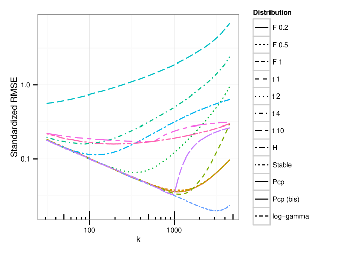
Figure 3: Monte-Carlo estimates of the standardised root mean square error (rmse) of Hill estimators as a function of the number of order statistics $k$ for samples of size $10000$ from the sampling distributions.

Index $\widehat{k}_{n}(r_{n})$ was computed according to the following rule

$$\widehat{k}_{n}(r_{n})=\min\left\{k\colon 30\leq k\leq n\text{ and }\exists i\in\{30,\ldots,k\}\,,\left|\widehat{\gamma}(i)-\widehat{\gamma}(k)\right|>\frac{r_{n}\widehat{\gamma}(i)}{\sqrt{i}}\right\}-1$$ (5.1)

with $r_{n}=\sqrt{c\ln\ln n}$ where $c=2.1$ unless otherwise specified.

The Fréchet, Student, $H$ and stable distributions all fit into the framework considered by (Drees and Kaufmann, 1998). They provide a favorable ground for comparing the performance of the optimal index selection method described by Drees and Kaufmann (1998) which attempts to take advantage of the second-order regular variation property and the performance of the simple selection rule described in this paper.

Index $\widehat{\gamma}(\widehat{k}^{\textsc{dk}}_{n})$ was computed following the recommandations from Theorem 1 and discussion in (Drees and Kaufmann, 1998)

$$\widehat{k}^{\textsc{dk}}_{n}=(2|\widehat{\rho}|+1)^{-1/|\widehat{\rho}|}\left(2\widehat{\rho}\widehat{\gamma}\right)^{1/(1+2|\hat{\rho}|)}\left(\frac{\widehat{k}_{n}(r_{n}^{\zeta})}{(\widehat{k}_{n}(r_{n}))^{\zeta}}\right)^{1/(1-\zeta)}$$ (5.2)

where $\widehat{\rho}$ should belong to a consistent family of estimators of $\rho$ (under a second-order regular variation assumption), $\widehat{\gamma}$ should be a preliminary estimator of $\gamma$ such as $\widehat{\gamma}(\sqrt{n})$, $\zeta=.7$, and $r_{n}=2n^{1/4}$. Following the advice from (Drees and Kaufmann, 1998), we replaced $|\widehat{\rho}|$ by $1$. Note that the method for computing $\widehat{k}^{\textsc{dk}}_{n}$ depends on a variety of tunable parameters.

Comparison between performances of $\widehat{\gamma}(\widehat{k}_{n}(r_{n}))$ and $\widehat{\gamma}(\widehat{k}_{n}^{\textsc{dk}})$ are reported in Tables 2 and 3. For each distribution from Table 1, for sample sizes $n=1000,2000,\text{ and }10000$, $5000$ experiments were replicated. As pointed out in (Drees and Kaufmann, 1998), on the sampling distributions that satisfy a second-order regular variation property, carefully tuned $\widehat{k}_{n}^{\textsc{dk}}$ is able to take advantage of it. Despite its computational and conceptual simplicity and the fact that it is almost parameter free, the estimator $\widehat{\gamma}(\widehat{k}_{n}(r_{n}))$ only suffers a moderate loss with respect to the oracle. When $|\rho|=1$, the observed ratios are of the same order as $(2\ln\ln n)^{1/3}\approx 1.65$. Moreover, whereas $\widehat{\gamma}(\widehat{k}_{n}^{\textsc{dk}})$ behaves erratically when facing Pareto change point distributions, $\widehat{\gamma}(\widehat{k}_{n}(r_{n}))$ behaves consistently.

Table 2: Ratios between median selected indices $\widehat{k}_{n}(r_{n})$ (Lepski), $\widehat{k}^{\textsc{dk}}_{n}$ (Drees-Kaufmann) and estimated oracle index $k_{n}^{*}$.

d.f.	$\gamma$	$\widehat{k}^{\textsc{dk}}_{n}/k_{n}^{*}$			$\widehat{k}_{n}(r_{n})/k_{n}^{*}$
		$n=1000$	2000	10000	1000	2000	10000
$F_{0.2}$	0.2	0.61	0.67	0.94	2.94	2.97	3.47
$F_{0.5}$	0.5	1.12	1.18	1.45	2.90	2.87	2.91
$F_{1}$	1	1.76	2.05	2.32	2.90	3.10	2.93
$t_{1}$	1	1.33	1.55	1.98	2.03	2.16	2.16
$t_{2}$	0.5	1.00	0.99	0.91	3.05	3.06	2.96
$t_{4}$	0.25	1.27	1.28	1.18	5.62	5.50	5.30
$t_{10}$	0.1	2.00	1.54	2.28	13.87	10.92	14.12
H	0.5	0.41	0.35	0.30	5.14	4.97	4.96
Stable	2	0.97	0.95	1.04	1.43	1.41	1.55
Pcp	1.5	1.85	0.45	0.15	1.32	1.21	1.10
Pcp (bis)	1.25	3.29	3.03	2.45	1.83	1.50	1.22
log-gamma	0.33	5.13	7.71	12.41	10.50	12.99	12.40

Table 3: Ratios between median rmse and median optimal rmse.

d.f.	$\gamma$	$\textsc{rmse}(\widehat{\gamma}(\widehat{k}^{\textsc{dk}}_{n}))/\textsc{rmse}(\widehat{\gamma}(k_{n}^{*}))$			$\textsc{rmse}(\widehat{\gamma}(\widehat{k}_{n}(r_{n})))/\textsc{rmse}(\widehat{\gamma}(k_{n}^{*}))$
		$n=1000$	2000	10000	1000	2000	10000
$F_{0.2}$	0.2	1.12	1.12	1.02	2.06	2.26	2.69
$F_{0.5}$	0.5	1.03	1.03	1.14	2.12	2.23	2.70
$F_{1}$	1	1.22	1.31	1.59	2.07	2.23	2.64
$t_{1}$	1	1.26	1.34	1.74	2.31	2.39	3.11
$t_{2}$	0.5	1.11	1.08	1.05	2.06	2.09	2.20
$t_{4}$	0.25	1.10	1.07	1.04	1.85	1.81	1.84
$t_{10}$	0.1	1.10	1.09	1.08	1.76	1.72	1.64
H	0.5	1.28	1.37	1.48	2.15	2.18	2.12
Stable	2	1.01	0.99	0.98	1.99	2.52	3.60
Pcp	1.5	4.25	1.66	2.52	2.50	2.68	3.63
Pcp (bis)	1.25	3.38	4.47	7.45	2.43	2.56	3.10
log-gamma	0.33	1.23	1.28	1.39	1.45	1.43	1.37

Figure 4 concisely describes the behaviour of the two index selection methods on samples from the Pareto change point distribution with parameters $\gamma=1.5,\gamma^{\prime}=1$ and threshold $\tau$ corresponding to the $1-1/15$ quantile. The plain line represents the standardised rmse of Hill estimators as a function of selected index. This figure contains the superposition of two density plots corresponding to $\widehat{k}^{\textsc{dk}}_{n}$ and $\widehat{k}(r_{n})$. The density plots were generated from $5000$ points with coordinates $(\widehat{k}(r_{n}),|\widehat{\gamma}(\widehat{k}(r_{n}))/\gamma-1|)$ and $5000$ points with coordinates $(\widehat{k}^{\textsc{dk}}_{n},|\widehat{\gamma}(\widehat{k}^{\textsc{dk}}_{n})/\gamma-1|)$. The contoured and well-concentrated density plot corresponds to the performance of $\widehat{\gamma}(\widehat{k}_{n})$. The diffuse tiled density plot corresponds to the performance of $\widehat{k}^{\textsc{dk}}_{n}$. Facing Pareto change point samples, the two selection methods behave differently. Lepski’s rule detects correctly an abrupt change at some point and selects an index slightly above that point. As the conditional bias varies sharply around the change point, this slight over estimation of the correct index still results in a significant loss as far as rmse is concerned. The Drees-Kaufmann rule, fed with an a priori estimate of the second-order parameter, picks out a much smaller index, and suffers a larger excess risk.

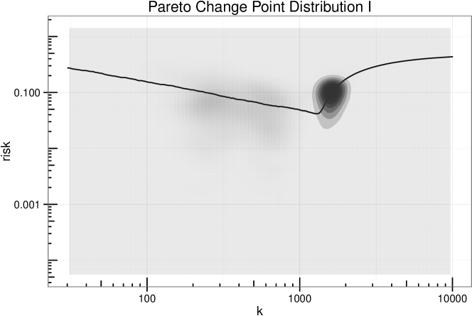
Figure 4: Risk plot for samples of size $10000$ from the Pareto change point distribution with parameters $\gamma=1.5,\gamma^{\prime}=1$ and threshold $\tau$ corresponding to the $1-1/15$ quantile. The concentrated density plot corresponds to points $(\widehat{k}(r_{n}),|\widehat{\gamma}(\widehat{k}(r_{n}))/\gamma-1|)$.

Acknowledgement The authors are thankful to the editor and the referees for their careful reading and valuable suggestions, which led to detect an error and to a improved version of the paper.

Appendix A Calibration of the preliminary selection rule

Darling and Erdös [1956] establish (among other things) that letting $Z_{n}$ denote $\sup_{k\leq n}\sum_{i=1}^{k}(E_{i}-1)/\sqrt{k}$, where $E_{i}$, $1\leq i\leq k$, are independent exponentially distributed random variables, the sequence $\sqrt{2\ln\ln n}\left(Z_{n}-\sqrt{2\ln\ln n}-\ln\ln\ln(n)/(2\sqrt{2\ln\ln n})\right)$ converges in distribution towards a translated Gumbel distribution. In other words, asymptotically, $Z_{n}$ behaves almost like the maximum of $\ln n$ independent standard Gaussian random variables.

Appendix B Proof of Corollary 2.16

Let $Z=g(E_{1},\ldots,E_{n})=\left(U\circ\exp\right)\left(\sum_{i=1}^{k}E_{i}/i\right)$. Then,

$$|\partial_{i}g|\leq\frac{1}{i}\sup_{x}\frac{1}{h(x)},\,\text{ for }i\geq k,$$

and

$$\|\nabla g\|^{2}=\sum_{i=k}^{n}\frac{1}{i^{2}}\frac{1}{(h\circ\ g)^{2}}\enspace.$$

Let $c<1$, then for all $\lambda,0\leq\lambda\leq c\,(k\inf_{x}h(x))$,

$$\ln\mathbb{E}\mathrm{e}^{\lambda(Z-\mathbb{E}Z)}\leq\frac{4/k\left(1+1/k\right)\mathbb{E}[1/h(Z)^{2}]\lambda^{2}}{2(1-c)}\,.$$

Now, start from the first statement in Theorem 2.15,

$$\operatorname{Ent}\left[\mathrm{e}^{\lambda(Z-\mathbb{E}Z)}\right] \leq \frac{2\lambda^{2}}{1-c}\mathbb{E}\left[\mathrm{e}^{\lambda(Z-\mathbb{E}Z)}\|\nabla f\|^{2}\right]$$

$$= \frac{4\lambda^{2}}{2(1-c)}\frac{1}{k}\left(1+\frac{1}{k}\right)\mathbb{E}\left[\frac{\mathrm{e}^{\lambda(Z-\mathbb{E}Z)}}{h(Z)^{2}}\right]$$

$$\leq \frac{4\lambda^{2}}{2(1-c)}\frac{1}{k}\left(1+\frac{1}{k}\right)\mathbb{E}\left[{\mathrm{e}^{\lambda(Z-\mathbb{E}Z)}}\right]\mathbb{E}\left[\frac{1}{h(Z)^{2}}\right]$$

where the last inequality follows from Chebychev negative association inequality. Hence,

$$\frac{\mathrm{d}}{\mathrm{d}\lambda}\left[\frac{1}{\lambda}\ln\mathbb{E}\mathrm{e}^{\lambda(Z-\mathbb{E}Z)}\right]=\frac{\operatorname{Ent}\left[\mathrm{e}^{\lambda(Z-\mathbb{E}Z)}\right]}{\lambda^{2}\mathbb{E}\left[\mathrm{e}^{\lambda(Z-\mathbb{E}Z)}\right]}\leq\frac{1}{2(1-c)}\frac{4}{k}\left(1+\frac{1}{k}\right)\mathbb{E}\left[\frac{1}{h(Z)^{2}}\right]\,.$$

This differential inequality is readily solved and leads to the corollary.

Appendix C Proof of Abelian Proposition 3.2

The proof proceeds by classical arguments. In the sequel, we use the almost sure representation argument. Without loss of generality, we assume that all the random variables live on the same probability space, and that, for any intermediate sequence $(k_{n})$, $\sqrt{k_{n}}(Y_{(k_{n}+1)}-\ln(n/k_{n}))$ converges almost surely towards a standard Gaussian random variable. Complemented with dominated convergence arguments, the next lemma will be the key element of the proof.

Lemma C.1.

Let $\eta\in\emph{{RV}}_{\rho},\rho\leq 0$ and $Y_{(k_{n}+1)}$ be the $(k_{n}+1)$th largest order statistic of a standard exponential sample, then, for any intermediate sequence $(k_{n})$ and $u>0$,

$$\lim_{n\to\infty}\frac{\eta(\mathrm{e}^{u+Y_{(k_{n}+1)}})}{\eta(n/k_{n})}=\mathrm{e}^{\rho u}\ \text{p.s}\enspace.$$

Proof.

Note that

$$\frac{\eta(\mathrm{e}^{u+Y_{(k_{n}+1)}})}{\eta(n/k_{n})} = \frac{\eta\Big{(}(n/k_{n})\mathrm{e}^{u+Y_{(k_{n}+1)}-\log(n/k_{n})}\Big{)}}{\eta(n/k_{n})}\,.$$

Then, the result follows since $Y_{(k_{n}+1)}-\log(n/k_{n})\overset{\text{p.s}}{\longrightarrow}0$ and the convergence $\eta(tx)/\eta(t)\rightarrow x^{\rho}$ is locally uniform on $(0,\infty)$. ∎

In order to secure dominated convergence arguments, we will use Drees’s improvement of Potter’s inequality [see de Haan and Ferreira, 2006, page 369]. For every $\epsilon,\delta>0$, there exists $t_{0}=t_{0}(\epsilon,\delta)$ such that, for $t,tx\geq t_{0}$,

$$\left|\eta(tx)/\eta(t)-x^{\rho}\right|\leq x^{\rho}\epsilon\max(x^{\delta},x^{-\delta})\,.$$ (C.2)

To prove Proposition 3.2, we start from Representation (2.4):

$$\widehat{\gamma}(k_{n})=\frac{1}{k_{n}}\sum_{i=1}^{k_{n}}\int_{0}^{E_{i}}\left(\gamma+\eta\left(\mathrm{e}^{u+Y_{(k_{n}+1)}}\right)\right)\mathrm{d}u\enspace.$$

By the Pythagorean relation,

$$\operatorname{Var}(\widehat{\gamma}(k_{n}))=\operatorname{Var}\left(\mathbb{E}[\widehat{\gamma}(k_{n})\mid Y_{(k_{n}+1)}]\right)+\mathbb{E}\left[\operatorname{Var}\left(\widehat{\gamma}(k_{n})\mid Y_{(k_{n}+1)}\right)\right]\,,$$

so that

$$\frac{k_{n}\operatorname{Var}(\widehat{\gamma}(k_{n}))-\gamma^{2}}{\eta\left(n/k_{n}\right)}$$

$$= \frac{k_{n}\operatorname{Var}\left(\mathbb{E}[\widehat{\gamma}(k_{n})\mid Y_{(k_{n}+1)}]\right)}{\eta(n/k_{n})}+k_{n}\mathbb{E}\left[\frac{\operatorname{Var}\left(\widehat{\gamma}(k_{n})\mid Y_{(k_{n}+1)}\right)-\frac{\gamma^{2}}{k_{n}}}{\eta(n/k_{n})}\right]\,.$$

The second summand can be further decomposed using (2.4).

$$\frac{k_{n}\operatorname{Var}(\widehat{\gamma}(k_{n}))-\gamma^{2}}{\eta\left(n/k_{n}\right)}$$

$$= \underbrace{\frac{k_{n}\operatorname{Var}\left(\mathbb{E}[\widehat{\gamma}(k_{n})\mid Y_{(k_{n}+1)}]\right)}{\eta(n/k_{n})}}_{\textsc{(i)}}$$

$$+\underbrace{\eta(\tfrac{n}{k_{n}})\mathbb{E}\left[\operatorname{Var}\left[\int_{0}^{E}\frac{\eta(\mathrm{e}^{u+Y_{(k_{n}+1)}})}{\eta(n/k_{n})}\mathrm{d}u\mid Y_{(k_{n}+1)}\right]\right]}_{(\textsc{ii})}$$

$$+\underbrace{2\gamma\mathbb{E}\left[\operatorname{Cov}\left[E,\int_{0}^{E}\frac{\eta(\mathrm{e}^{u+Y_{(k_{n}+1)}})}{\eta(n/k_{n})}\mathrm{d}u\mid Y_{(k_{n}+1)}\right]\right]}_{(\textsc{iii})}.$$

We check that (i) and (ii) tend to $0$ and then that (iii) converges towards a finite limit.

Fix $\epsilon,\delta>0$ and define $M=\sup\{\eta(t),t\leq t_{0}\}$.
Let $A_{n}$ denote the event $\{Y_{(k_{n}+1)}>\ln t_{0}(\epsilon,\delta)\}$. For $n$ such that $\ln(n/k_{n})\leq 2\ln t_{0}$, as $Y_{(k_{n}+1)}$ is sub-gamma with variance factor $1/k_{n}$,

$$\mathbb{P}\{A^{c}_{n}\}\leq\exp\left(-k_{n}(\ln(n/k_{n}))^{2}/8\right)\,.$$

We first check that (ii) tends to $0$. Let $n$ be such that $n/k_{n}\geq t_{0}$ and $W_{n}$ denote the random variable $Y_{(k_{n}+1)}-\ln\left(n/k_{n}\right)$. Note that, for $0\leq\lambda\leq k_{n}/2$,

$$\mathbb{E}\mathrm{e}^{\lambda|W_{n}|}\leq 2\mathrm{e}^{\frac{\lambda^{2}}{k_{n}}}\,.$$

Using Jensen’s inequality and Fubini’s Theorem,

$$\mathbb{E}\left[\operatorname{Var}\left[\int_{0}^{E}\frac{\eta(\mathrm{e}^{u+Y_{(k_{n}+1)}})}{\eta(n/k_{n})}\mathrm{d}u\mid Y_{(k_{n}+1)}\right]\right]$$

$$\leq \mathbb{E}\left[\mathbb{E}\left[E\int_{0}^{E}\left(\frac{\eta(\mathrm{e}^{u+Y_{(k_{n}+1)}})}{\eta(n/k_{n})}\right)^{2}\mathrm{d}u\mid Y_{(k_{n}+1)}\right]\right]$$

$$= \int_{0}^{\infty}\mathrm{e}^{-v}v\int_{0}^{v}\mathbb{E}\left[\left(\frac{\eta(\mathrm{e}^{u+Y_{(k_{n}+1)}})}{\eta(n/k_{n})}\right)^{2}\right]\mathrm{d}u\mathrm{d}v$$

$$= \int_{0}^{\infty}\mathrm{e}^{-v}v\int_{0}^{v}\mathbb{E}\left[\left(\frac{\eta(\mathrm{e}^{u+W_{n}}n/k_{n})}{\eta(n/k_{n})}\right)^{2}\right]\mathrm{d}u\mathrm{d}v$$

We now apply Potter’s inequality (C.2) on the event $A_{n}$ with $t=n/k_{n}>t_{0}$ and $tx=\mathrm{e}^{u+Y_{(k_{n}+1)}}>t_{0},u>0$ :

$$\mathbb{E}\left[\operatorname{Var}\left[\int_{0}^{E}\frac{\eta(\mathrm{e}^{u+Y_{(k_{n}+1)}})}{\eta(n/k_{n})}\mathrm{d}u\mid Y_{(k_{n}+1)}\right]\right]$$

$$\leq \int_{0}^{\infty}\mathrm{e}^{-v}v\int_{0}^{v}\mathbb{E}\left[\mathbb{1}_{A_{n}}\mathrm{e}^{2\rho(u+W_{n})}\left(1+\epsilon\mathrm{e}^{\delta(u+|W_{n}|)}\right)^{2}+\mathbb{1}_{A_{n}^{c}}\frac{M^{2}}{\eta(n/k_{n})^{2}}\right]\mathrm{d}u\mathrm{d}v$$

$$\leq \int_{0}^{\infty}\mathrm{e}^{-v}v\int_{0}^{v}\mathbb{E}\left[\mathrm{e}^{2\rho W_{n}}2\left(1+\epsilon^{2}\mathrm{e}^{2\delta(u+|W_{n}|)}\right)\right]\mathrm{d}u\mathrm{d}v+\frac{2M^{2}}{\eta(n/k_{n})^{2}}\mathbb{E}\mathbb{1}_{A_{n}^{c}}\,.$$

The first summand has a finite limit thanks to Lemma C.1. The second summand converges to $0$ as $\mathbb{E}\mathbb{1}_{A_{n}^{c}}$ tends to $0$ exponentially fast while $1/\eta(n/k_{n})^{2}$ tends to infinity algebraically fast.

Bounds on (i) are easily obtained, using Jensen’s Inequality and Poincaré Inequality.

$$\frac{k_{n}\operatorname{Var}\left(\mathbb{E}[\widehat{\gamma}(k_{n})\mid Y_{(k_{n}+1)}]\right)}{\eta(n/k_{n})} = \frac{k_{n}\operatorname{Var}\left(\int_{0}^{\infty}{\eta\left(\mathrm{e}^{u+Y_{(k_{n}+1)}}\right)}\mathrm{e}^{-u}\mathrm{d}u\right)}{\eta(n/k_{n})}$$

$$\leq 4\eta(n/k_{n})\mathbb{E}\left[\left(\int_{0}^{\infty}\frac{\eta\left(\mathrm{e}^{u+Y_{(k_{n}+1)}}\right)}{\eta(n/k_{n})}\mathrm{e}^{-u}\mathrm{d}u\right)^{2}\right]$$

$$\leq 4\eta(n/k_{n})\mathbb{E}\left[\int_{0}^{\infty}\left(\frac{\eta\left(\mathrm{e}^{u+Y_{(k_{n}+1)}}\right)}{\eta(n/k_{n})}\right)^{2}\mathrm{e}^{-u}\mathrm{d}u\right]\,.$$

Using the line of arguments as for handling the limit of (ii), we establish that (i) converges to $0$.

We now check that (iii) converges towards a finite limit. Note that

$$\mathbb{E}\left[\operatorname{Cov}\left[E,\int_{0}^{E}\frac{\eta(\mathrm{e}^{u+Y_{(k_{n}+1)}})}{\eta(n/k_{n})}\mathrm{d}u\mid Y_{(k_{n}+1)}\right]\right]$$

$$= \mathbb{E}\left[(E-1)\int_{0}^{E}\frac{\eta(\mathrm{e}^{u+Y_{(k_{n}+1)}})}{\eta(n/k_{n})}\mathrm{d}u\right]\,.$$

By Lemma C.1, for almost every $u>0$,

$$(E-1)\frac{\eta(\mathrm{e}^{u+W_{n}}n/k_{n})}{\eta(n/k_{n})}\underset{n\to\infty}{\longrightarrow}(E-1)\mathrm{e}^{\rho u}\,,$$

and

$$\lvert E-1\rvert\int_{0}^{E}\left|\frac{\eta(\mathrm{e}^{u+W_{n}}n/k_{n})}{\eta(n/k_{n})}\right|\mathrm{d}u$$

$$\leq |E-1|\int_{0}^{E}\mathrm{e}^{\rho(u+W_{n})}\left(1+\epsilon\mathrm{e}^{\delta(u+|W_{n}|)}\right)\mathrm{d}u+\mathbb{1}_{A_{n}^{c}}E|E-1|\frac{M}{|\eta(n/k_{n})|}\enspace.$$

The first term is finite as the integral of a continuous function on a compact.
Thus,

$$(E-1)\int_{0}^{E}\frac{\eta(\mathrm{e}^{u+W_{n}}n/k_{n})}{\eta(n/k_{n})}\mathrm{d}u\rightarrow_{n}(E-1)\int_{0}^{E}\mathrm{e}^{\rho u}\mathrm{d}u=(E-1)\frac{\mathrm{e}^{\rho E}-1}{\rho}\,.$$

The expected value of the last random variable is $1/(1-\rho)^{2}$.

We check that, for sufficiently large $n$,

$$\mathbb{E}\left[|E-1|\int_{0}^{E}\frac{|\eta(\mathrm{e}^{u+W_{n}}n/k_{n})|}{|\eta(n/k_{n})|}\mathrm{d}u\right]$$

$$\leq \mathbb{E}\left[|E-1|\int_{0}^{E}\mathrm{e}^{\rho(u+W_{n})}\left(1+\epsilon\mathrm{e}^{\delta(u+|W_{n}|)}\right)+\mathbb{1}_{A_{n}^{c}}|E-1|\frac{M}{|\eta(n/k_{n})|}\mathrm{d}u\right]$$

$$\leq \mathbb{E}\left[\mathrm{e}^{\rho W_{n}}\left(2+\frac{\epsilon}{\delta(1-\delta)^{2}}\mathrm{e}^{\delta|W_{n}|}\right)\right]+\frac{M}{|\eta(n/k_{n})|}\mathbb{E}\mathbb{1}_{A_{n}^{c}}$$

$$\leq 4\mathrm{e}^{\frac{\rho^{2}}{k_{n}}}+\frac{2\epsilon}{\delta(1-\delta)^{2}}\mathrm{e}^{\frac{(\delta-\rho)^{2}}{k_{n}}}+\frac{M}{|\eta(n/k_{n})|}\mathbb{E}\mathbb{1}_{A_{n}^{c}}\enspace.$$

We now way conclude by dominated convergence that

$$\textsc{(iii)}\underset{n\to\infty}{\longrightarrow}\frac{2\gamma}{(1-\rho)^{2}}\enspace.$$

Appendix D Proof of Proposition 4.6

The proof of Proposition 4.3 from [Boucheron and Thomas, 2012] yields that, with probability larger than $1-\delta$, for $0\leq z$,

$$\mathbb{P}\left\{\exp\left(Y_{(k+1)}\right)\geq\frac{n}{k}\mathrm{e}^{-z}\right\}\geq 1-\exp\left(-2k\sinh\left({z}/{2}\right)^{2}\right)\,.$$

We may choose $z=2\operatorname{arsinh}(\sqrt{{\ln\left(1/\delta\right)}/{2k}})$ and notice that $\operatorname{arsinh}(x)=\ln(x+\sqrt{1+x^{2}})$. This yields

$$\mathrm{e}^{z}\leq 1+2\frac{\ln\left(1/\delta\right)}{k}+\sqrt{\frac{2\ln(1/\delta)}{k}}\quad\text{ and }\quad\exp\left(-2k\sinh\left({z}/{2}\right)^{2}\right)=\delta\,.$$

Appendix E Revisiting the lower bound on adaptive estimation error

Lower bounds on tail index estimation error [Drees, 2001, 1998a, Novak, 2014, Carpentier and Kim, 2015] are usually constructed by defining sequences of local models around a pure Pareto distribution with shape parameter $\gamma_{0}$. When deriving lower bounds for the estimation error under constraints like $\overline{\eta}$ is regularly varying, the elements of the local model for sample size $n$ may be defined by

$$U_{n,h}(t)=t^{\gamma_{0}+d_{n}h(0)}\exp\int_{1}^{t}d_{n}\frac{h(c_{n}/s)-h(0)}{s}\mathrm{d}s$$

where $h$ is square integrable over $[0,1]$, $d_{n}\rightarrow 0$, $nd_{n}^{2}/c_{n}\rightarrow 1$ [Drees, 2001]. The sequences $d_{n}$ and $c_{n}$ are chosen in such a way that $d_{n}\left|h(c_{n}/s)-h(0)\right|=|\overline{\eta}(s)|$ satisfies the required constraint. If the local alternatives are Pareto change point distributions as in [Novak, 2014] and [Carpentier and Kim, 2015], $h(x)=\mathbb{1}_{\{x\leq 1\}}$, $c_{n}=\tau_{n}^{1/\gamma_{0}}$. Drees [2001] explores a richer collection of local alternatives in order to fit into the theory of weak convergence of local experiments.

In order to explore adaptivity as in [Carpentier and Kim, 2015], it is necessary to handle simultaneously a collection of sequences $(d_{n},c_{n})_{n}$ corresponding to different rates of decay of the von Mises function. The difficulty of estimation is connected with the difficulty of distinguishing alternatives with different tail indices that is, with the hardness of a multiple hypotheses testing problem. In order to lower bound the testing error, Carpentier and Kim chose to use Fano’s Lemma [Cover and Thomas, 1991, see]. Using Fano’s Lemma requires bounding the Kullback-Leibler divergence between the different local alternatives which is not as easy as bounding the divergence between a Pareto change point distribution and a pure Pareto distribution.

The next lemma is from [Birgé, 2005]. It can be used in the derivation of risk lower bounds instead of the classical Fano Lemma. Just as Fano’s Lemma, it states a lower bound on the error in multiple hypothesis testing. However, as it only requires computing the Kullback-Leibler divergence to the localisation center, in the present setting, it significantly alleviates computations and makes the proof more concise and more transparent.

Lemma E.1.

(Birgé-Fano) Let $P_{0},\ldots,P_{M}$ be a collection of probability distributions on some space, and let $A_{0},\ldots,A_{M}$ be a collection of pairwise disjoint events, then the following holds

$$\min_{i}P_{i}\{A_{i}\}\leq\frac{2\mathrm{e}}{1+2\mathrm{e}}\vee\frac{\frac{1}{M}\sum_{i=1}^{M}\mathcal{K}(P_{i},P_{0})}{\ln(M+1)}\,.$$

In order to take advantage of Lemma E.1, we use the Bayesian game designed in [Carpentier and Kim, 2015].

Theorem E.2.

Let $\gamma>0$, $\rho<-1$, and $0\leq v\leq\mathrm{e}/(1+2\mathrm{e})$. Then, for any tail index estimator $\widehat{\gamma}$ and any sample size $n$ such that $M=\lfloor\ln n\rfloor>\mathrm{e}^{1/v}$, there exists a collection $(P_{i})_{i\leq M}$ of probability distributions such that

1. $P_{i}\in\emph{{MDA}}(\gamma_{i})$ with $\gamma_{i}>\gamma$,

2. $P_{i}$ meets the von Mises condition with von Mises function $\eta_{i}$ satisfying

   $$\overline{\eta}_{i}(t)\leq\gamma t^{\rho_{i}}$$

   where $\rho_{i}=\rho+i/M<0$,

3. $$\max_{i\leq M}P^{\otimes n}_{i}\left\{|\widehat{\gamma}-\gamma_{i}|\geq\frac{C_{\rho}}{4}\gamma_{i}\left(\frac{v\ln\ln n}{n}\right)^{|\rho_{i}|/(1+2|\rho_{i}|)}\right\}\geq\frac{1}{1+2\mathrm{e}}$$

   and

   $$\max_{i\leq M}\mathbb{E}_{P^{\otimes n}_{i}}\left[\frac{|\widehat{\gamma}-\gamma_{i}|}{\gamma_{i}}\right]\geq\frac{C_{\rho}}{4(1+2\mathrm{e})}\left(\frac{v\ln\ln n}{n}\right)^{|\rho|/(1+2|\rho|)}\,,$$

   with $C_{\rho}=1-\exp\left(-\tfrac{1}{2(1+2|\rho|)^{2}}\right)$.

Proof of Theorem E.2.

Choose $v$ so that $0\leq v\leq 2\mathrm{e}/(1+2\mathrm{e})$. The number of alternative hypotheses $M$ is chosen in such a way that $M/2\leq\ln\left(n/(v\ln M)\right)\leq M$. If $\lfloor\ln n\rfloor\geq\mathrm{e}^{1/v}$, $M=\lfloor\ln n\rfloor$ will do.

The center of localisation $P_{0}$ is the pure Pareto distribution with shape parameter $\gamma>0$ ($P_{0}\{(\tau,\infty)\}=\tau^{-1/\gamma}$). The local alternatives $P_{1},\ldots,P_{M}$ are Pareto change point distributions. Each $P_{i}$ is defined by a breakpoint $\tau_{i}>1$ and an ultimate Pareto index $\gamma_{i}$. If $F_{i}$ denotes the distribution function of $P_{i}$,

$$\overline{F}_{i}(x)=x^{-1/\gamma}\mathbb{1}_{\{1\leq x\leq\tau_{i}\}}+\tau_{i}^{-1/\gamma}(x/\tau_{i})^{-1/\gamma_{i}}\mathbb{1}_{\{x\geq\tau_{i}\}}\,.$$

Karamata’s representation of $(1/\overline{F}_{i})^{\leftarrow}$ is

$$U_{i}(t)=t^{\gamma_{i}}\exp\left(\int_{1}^{t}\frac{\eta_{i}(s)}{s}\right)\mathrm{d}s$$

with $\eta_{i}(s)=(\gamma-\gamma_{i})\mathbb{1}_{\{s\leq\tau_{i}^{1/\gamma}\}}\,.$

The Kullback-Leibler divergence between $P_{i}$ and $P_{0}$ is readily calculated,

$$\mathcal{K}(P_{i},P_{0})=\overline{F}_{i}(\tau_{i})\left(\frac{\gamma_{i}}{\gamma}-1-\ln\frac{\gamma_{i}}{\gamma}\right)=\tau_{i}^{-1/\gamma}\left(\frac{\gamma_{i}}{\gamma}-1-\ln\frac{\gamma_{i}}{\gamma}\right)\,.$$

If $\gamma_{i}>\gamma$, the next upper bound holds,

$$\mathcal{K}(P_{i},P_{0})\leq\frac{\tau_{i}^{-1/\gamma}}{2}\left(\frac{\gamma_{i}}{\gamma}-1\right)^{2}\,.$$

The breakpoints and tail indices are chosen in such a way that all upper bounds are equal (namely $n\tau_{i}^{-1/\gamma}(\gamma_{i}/\gamma-1)^{2}$ does not depend on $i$),

$$\tau_{i} = \left(n/(v\ln M)\right)^{\gamma/(1+2|\rho_{i}|)}$$

$$\gamma_{i} = \gamma+\gamma\left(n/(v\ln M)\right)^{\rho_{i}/(1+2|\rho_{i}|)}\,,$$

so that $\mathcal{K}(P_{i}^{\otimes n},P_{0}^{\otimes n})=n\mathcal{K}(P_{i},P_{0})\leq{v\ln M}$, for all $1\leq i\leq M$.

Note that, for all $t>1$,

$$|\eta_{i}(t)|=|\gamma-\gamma_{i}|\mathbb{1}_{\{t\leq\tau_{i}^{1/\gamma}\}}\leq\gamma\tau_{i}^{\rho_{i}/\gamma}\mathbb{1}_{\{t\leq\tau_{i}^{1/\gamma}\}}\leq\gamma t^{\rho_{i}}$$

the upper bound being achieved at $t=\tau_{i}^{1/\gamma}.$

Now, let $\widehat{\gamma}$ be any tail index estimator. Define region $A_{i}$, as the set of samples such that $\gamma_{i}$ minimises $|\widehat{\gamma}-\gamma_{j}|$, for $1\leq j\leq M$. Then, if the event $A_{i}$ is not realised,

$$|\widehat{\gamma}-\gamma_{i}|\geq\frac{1}{2}\min_{1\leq j\leq M,j\neq i}|\gamma_{j}-\gamma_{i}|\,.$$

By Birgé’s Lemma,

$$\max_{i\leq M}\mathbb{P}_{i}^{\otimes n}\left\{|\widehat{\gamma}-\gamma_{i}|\geq\frac{1}{2}\min_{1\leq j\leq M,j\neq i}|\gamma_{j}-\gamma_{i}|\right\}\geq\frac{1}{1+2\mathrm{e}}\,.$$

In order to make the whole construction useful, it remains to choose the “second-order parameters” $\rho_{i}$’s (the true second-order parameter of each $P_{i}$ is infinite!). We will need an upper bound on $\gamma_{i}/\gamma$ (but we already have $\gamma_{i}/\gamma\leq 2$), as well as a lower bound on ${|\gamma_{j}-\gamma_{i}|}/{\gamma}$ for $j\neq i$ that scales like $\left({n}/{\ln\ln n}\right)^{\rho_{i}/(1+2|\rho_{i}|)}$.

Following Carpentier and Kim [2015], we finally choose $\rho_{i}$ as $\rho_{i}=\rho+i/M$ for $1\leq i\leq M$. Then, for $j<i$, using that $M/2\leq\ln(n/(v\ln M))\leq M$ and $\rho_{i}-\rho_{j}=(i-j)/M$,

$$\frac{|\gamma_{j}-\gamma_{i}|}{\gamma_{i}}$$

$$\geq \frac{|\gamma_{j}-\gamma_{i}|}{2\gamma}$$

$$\geq \frac{1}{2}\left(\frac{n}{v\ln M}\right)^{\rho_{i}/(1+2|\rho_{i}|)}\left|1-\left(\frac{n}{v\ln M}\right)^{\rho_{j}/(1+2|\rho_{j}|)-\rho_{i}/(1+2|\rho_{i}|)}\right|$$

$$\geq \frac{1}{2}\left(\frac{n}{v\ln M}\right)^{\rho_{i}/(1+2|\rho_{i}|)}\left[1-\exp\left(\frac{-(i-j)}{M(1+2|\rho_{i}|)(1+2|\rho_{j}|)}\ln\left(\frac{n}{v\ln M}\right)\right)\right]$$

$$\geq \frac{1}{2}\left(\frac{n}{v\ln M}\right)^{\rho_{i}/(1+2|\rho_{i}|)}\left[1-\exp\left(\frac{-(i-j)}{2(1+2|\rho_{i}|)(1+2|\rho_{j}|)}\right)\right]$$

$$\geq \frac{C_{\rho}}{2}\left(\frac{n}{v\ln M}\right)^{\rho_{i}/(1+2|\rho_{i}|)}$$

where $C_{\rho}$ may be chosen as $1-\exp\left(-\tfrac{1}{2(1+2|\rho|)^{2}}\right)$. ∎

References

• Beirlant et al. [2004] J. Beirlant, Y. Goegebeur, J. Teugels, and J. Segers. Statistics of extremes. John Wiley & Sons, Ltd., 2004.
• Beirlant et al. [2006] J. Beirlant, C. Bouquiaux, and B. Werker. Semiparametric lower bounds for tail index estimation. Journal of Statistical Planning and Inference, 136(3):705–729, 2006.
• Bingham et al. [1987] N. Bingham, C. Goldie, and J. Teugels. Regular variation. Cambridge University Press, 1987.
• Birgé [2001] L. Birgé. An alternative point of view on Lepski’s method. In State of the art in probability and statistics (Leiden, 1999), volume 36 of IMS Lecture Notes Monogr. Ser., pages 113–133. Inst. Math. Statist., 2001.
• Birgé [2005] L. Birgé. A new lower bound for multiple hypothesis testing. IEEE Trans. Inform. Theory, 51:1611–1615, 2005.
• Bobkov and Ledoux [1997] S. Bobkov and M. Ledoux. Poincaré’s inequalities and Talagrand’s concentration phenomenon for the exponential distribution. Probab. Theory Rel. Fields, 107:383–400, 1997.
• Boucheron and Thomas [2012] S. Boucheron and M. Thomas. Concentration inequalities for order statistics. Elec. Commun. Probab., 17:1–12, 2012.
• Boucheron et al. [2013] S. Boucheron, G. Lugosi, and P. Massart. Concentration inequalities. Oxford University Press, 2013.
• Carpentier and Kim [2014] A. Carpentier and A. Kim. Adaptive confidence intervals for the tail coefficient in a wide second order class of pareto models. Elec. Journ. Statist., 8:2066–2110, 2014.
• Carpentier and Kim [2015] A. Carpentier and A. Kim. Adaptive and minimax optimal estimation of the tail coefficient. Statistica Sinica, 25:1133–1144, 2015.
• Chatterjee [2014] S. Chatterjee. Superconcentration and related topics. Springer-Verlag, 2014.
• Cover and Thomas [1991] T. Cover and J. Thomas. Elements of Information Theory. John Wiley, 1991.
• Csörgő et al. [1985] S. Csörgő, P. Deheuvels, and D. Mason. Kernel estimates of the tail index of a distribution. Ann. Statist., 13(3):1050–1077, 1985.
• Danielsson et al. [2001] J. Danielsson, L. de Haan, L. Peng, and C. G. de Vries. Using a bootstrap method to choose the sample fraction in tail index estimation. J. Multivariate Anal., 76(2):226–248, 2001.
• Darling and Erdös [1956] D. Darling and P. Erdös. A limit theorem for the maximum of normalized sums of independent random variables. Duke Math. J, 23:143–155, 1956.
• de Haan and Ferreira [2006] L. de Haan and A. Ferreira. Extreme value theory. Springer-Verlag, 2006.
• Draisma et al. [1999] G. Draisma, L. de Haan, L. Peng, and T. Pereira. A bootstrap-based method to achieve optimally in estimating the extreme value index. Extremes, 2:367–404, 1999.
• Drees [1998a] H. Drees. Optimal rates of convergence for estimates of the extreme value index. Ann. Statist., 26(1):434–448, 1998a.
• Drees [1998b] H. Drees. On smooth statistical tail functionals. Scand. J. Statist., 25(1):187–210, 1998b.
• Drees [2001] H. Drees. Minimax risk bounds in extreme value theory. Ann. Statist., 29(1):266–294, 2001.
• Drees and Kaufmann [1998] H. Drees and E. Kaufmann. Selecting the optimal sample fraction in univariate extreme value estimation. Stochastic Process. Appl., 75(2):149–172, 1998.
• Drees et al. [2000] H. Drees, L. De Haan, and S. Resnick. How to make a Hill plot. Ann. Statist., 28(1):254–274, 2000.
• Geluk et al. [1997] J. Geluk, L. de Haan, S. Resnick, and C. Stărică. Second-order regular variation, convolution and the central limit theorem. Stochastic Process. Appl., 69(2):139–159, 1997.
• Giné and Koltchinskii [2006] E. Giné and V. Koltchinskii. Concentration inequalities and asymptotic results for ratio type empirical processes. Ann. Probab., 34(3):1143–1216, 2006.
• Grama and Spokoiny [2008] I. Grama and V. Spokoiny. Statistics of extremes by oracle estimation. Ann. Statist., 36(4):1619–1648, 2008.
• Hall and Weissman [1997] P. Hall and I. Weissman. On the estimation of extreme tail probabilities. Ann. Statist., 25(3):1311–1326, 1997.
• Hall and Welsh [1985] P. Hall and A. Welsh. Adaptive estimates of parameters of regular variation. Ann. Statist., 13(1):331–341, 1985.
• Hill [1975] B. Hill. A simple general approach to inference about the tail of a distribution. Ann. Statist., 3:1163–1174, 1975.
• Koltchinskii [2008] V. Koltchinskii. Oracle inequalities in empirical risk minimization and sparse recovery problems. Ecole d’Eté de Probabilité de Saint-Flour xxxviii, volume 2033 of Lecture Notes in Math.. Springer-Verlag, 2008.
• Ledoux [2001] M. Ledoux. The concentration of measure phenomenon. American Mathematical Society, 2001.
• Ledoux and Talagrand [1991] M. Ledoux and M. Talagrand. Probability in Banach Space. Springer-Verlag, 1991.
• Lepski [1990] O. Lepski. A problem of adaptive estimation in Gaussian white noise. Teoriya Veroyatnosteui i ee Primeneniya, 35(3):459–470, 1990.
• Lepski [1991] O. Lepski. Asymptotically minimax adaptive estimation. I. Upper bounds. Optimally adaptive estimates. Teoriya Veroyatnosteui i ee Primeneniya, 36(4):645–659, 1991.
• Lepski [1992] O. Lepski. Asymptotically minimax adaptive estimation. II. Schemes without optimal adaptation. Adaptive estimates. Teoriya Veroyatnosteui i ee Primeneniya, 37(3):468–481, 1992.
• Lepski and Tsybakov [2000] O. Lepski and A. Tsybakov. Asymptotic exact nonparametric hypothesis testing in sup-norm and at a fixed point. Probab. Theory Rel. Fields, 117(1):17–48, 2000.
• Mason [1982] D. Mason. Laws of large numbers for sums of extreme values. Ann. Probab., 10:754–764, 1982.
• Massart [2007] P. Massart. Concentration inequalities and model selection. Ecole d’Eté de Probabilité de Saint-Flour xxxiv, volume 1896 of Lecture Notes in Math.. Springer-Verlag, 2007.
• Mathé [2006] P. Mathé. The Lepski principle revisited. Inverse Problems, 22(3):L11–L15, 2006.
• Maurey [1991] B. Maurey. Some deviation inequalities. Geometric and Functional Analysis, 1(2):188–197, 1991.
• Novak [2014] S. Novak. Lower bounds to the accuracy of inference on heavy tails. Bernoulli, 20(2):979–989, 2014.
• Resnick [2007] S. Resnick. Heavy-tail phenomena: probabilistic and statistical modeling, Springer-Verlag, 2007.
• Segers [2002] J. Segers. Abelian and Tauberian theorems on the bias of the Hill estimator. Scand. J. Statist., 29(3):461–483, 2002.
• Talagrand [1991] M. Talagrand. A new isoperimetric inequality and the concentration of measure phenomenon. In Geometric aspects of functional analysis (1989–90), volume 1469 of Lecture Notes in Math., pages 94–124. Springer-Verlag, 1991.
• Talagrand [1996a] M. Talagrand. A new look at independence. Ann. Probab., 24:1–34, 1996a.
• Talagrand [1996b] M. Talagrand. New concentration inequalities in product spaces. Inventiones Mathematicae, 126:505–563, 1996b.
• Talagrand [2005] M. Talagrand. The generic chaining. Springer-Verlag, 2005.
• Tsybakov [1998] A. B. Tsybakov. Pointwise and sup-norm sharp adaptive estimation of functions on the Sobolev classes. Ann. Statist., 26(6):2420–2469, 1998.
• van de Geer [2000] S. van de Geer. Applications of empirical process theory. Cambridge University Press, 2000.
• Wickham [2009] H. Wickham. ggplot2: elegant graphics for data analysis. Springer-Verlag, 2009.
• Wickham [2014] H. Wickham. Advanced R. Chapman & Hall/CRC, 2014.