Learning Models for Following Natural Language Directions
in Unknown Environments

Abstract

Natural language offers an intuitive and flexible means for humans to communicate with the robots that we will increasingly work alongside in our homes and workplaces. Recent advancements have given rise to robots that are able to interpret natural language manipulation and navigation commands, but these methods require a prior map of the robot’s environment. In this paper, we propose a novel learning framework that enables robots to successfully follow natural language route directions without any previous knowledge of the environment. The algorithm utilizes spatial and semantic information that the human conveys through the command to learn a distribution over the metric and semantic properties of spatially extended environments. Our method uses this distribution in place of the latent world model and interprets the natural language instruction as a distribution over the intended behavior. A novel belief space planner reasons directly over the map and behavior distributions to solve for a policy using imitation learning. We evaluate our framework on a voice-commandable wheelchair. The results demonstrate that by learning and performing inference over a latent environment model, the algorithm is able to successfully follow natural language route directions within novel, extended environments.

I Introduction

Over the past decade, robots have moved out of controlled isolation and into our homes and workplaces, where they coexist with people in domains that include healthcare and manufacturing. One long-standing challenge to realizing robots that behave effectively as our partners is to develop command and control mechanisms that are both intuitive and efficient. Natural language offers a flexible medium through which people can communicate with robots, without requiring specialized interfaces or significant prior training. For example, a voice-commandable wheelchair [1] allows the mobility-impaired to independently and safely navigate their surroundings simply by speaking to the chair, without the need for traditional head-actuated switches or sip-and-puff arrays. Recognizing these advantages, much attention has been paid of late to developing algorithms that enable robots to interpret natural language expressions that provide route directions [2, 3, 4, 5], that command manipulation [6, 7], and that convey environment knowledge [8, 9].

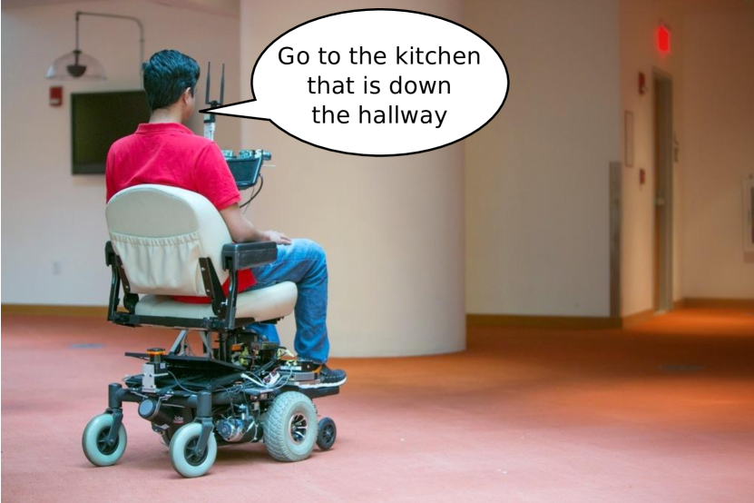
Figure 1: Our goal is to enable robots to autonomously follow natural language commands without any prior knowledge of their environment.

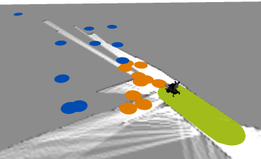
(a)

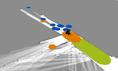
(b)

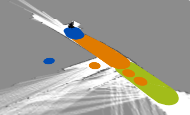
(c) $t=8$

Figure 2: Visualization of the evolution of the semantic map over time as the robot follows the command “go to the kitchen that is down the hallway.” Small circles and large filled-in areas denote sampled and visited regions, respectively, each colored according to its type (lab: green, hallway: yellow, kitchen: blue). The robot (a) first samples possible locations of the kitchen and moves towards them, (b) then observes the hallway and refines its estimate using the “down” relation provided by the user. Finally, the robot (c) reaches the actual kitchen and declares it has finished following the direction.

Natural language interpretation becomes particularly challenging when the expression references areas in the environment unknown to the robot. Consider an example in which a user directs the voice-commandable to “go to the kitchen that is down the hallway,” when the wheelchair is in an unknown environment and the hallway and kitchen are outside the field-of-view of its sensors (Fig. 1). Unable to associate the hallway and kitchen with specific locations, most existing solutions to language understanding would result in the robot exploring until it happens upon a kitchen. By reasoning over the spatial and semantic environment information that the command conveys, however, the robot would be able to follow the spoken directions more efficiently.

In this paper, we propose a framework that follows natural language route directions within unknown environments by exploiting spatial and semantic knowledge implicit in the commands. There are three algorithmic contributions that are integral to our approach. The first is a learned language understanding model that efficiently infers environment annotations and desired behaviors from the user’s command. The second is an estimation-theoretic algorithm that learns a distribution over hypothesized world models by treating the inferred annotations as observations of the environment and fusing them as observations from the robot’s sensor streams (Fig. 2). The third is a belief space policy learned from human demonstrations that reasons directly over the world model distribution to identify suitable navigation actions.

This paper generalizes previous work by the authors [10], which was limited to object-relative navigation within small, open environments. The novel contributions of this work enable robots to follow natural language route directions in large, complex environments. They include: a hierarchical framework that learns a compact probabilistic graphical model for language understanding; a semantic map inference algorithm that hypothesizes the existence and location of regions in spatially extended environments; and a belief space policy learned from human demonstrations that considers spatial relationships with respect to a hypothesized map distribution. We demonstrate these advantages through simulations and experiments with a voice-commandable wheelchair in an office-like environment.

II Related Work

Recent advancements in language understanding have enabled robots to understand free-form commands that instruct them to manipulate objects [6, 7] or navigate through environments using route directions [2, 3, 4, 7, 11]. With few exceptions, most of these techniques require a priori knowledge of location, geometry, colloquial name, and type of all objects and regions within the environment [3, 7, 6]. Without known world models, however, interpreting free-form commands becomes much more difficult. Existing methods have dealt with this by learning a parser that maps the natural language command directly to plans [2, 4, 11]. Alternatively, Duvallet et al. [12] use imitation learning to train a policy that reasons about uncertainty in the grounding and that is able to backtrack as necessary. However, none of these approaches explicitly utilize the knowledge that the instruction conveys to influence their models of the environment, nor do they reason about its uncertainty. Instead, our framework treats language as an additional, albeit noisy, sensor that we use to learn a distribution over hypothesized world models, by taking advantage of information implicitly contained in a given command.

Related to our algorithm’s ability to learn world models, state-of-the-art semantic mapping frameworks exist that focus on using the robot’s sensor observations to update its representation of the world [13, 14]. Some methods additionally incorporate natural language descriptions in order to improve the learned world models [8, 9]. These techniques, however, only use language to update regions of the environment that the robot has observed and are not able to extend the maps based on natural language. Our approach treats natural language as another sensor and uses it to extend the spatial representation by adding both topological and metric information regarding hypothesized regions in the environment, which is then used for planning. Williams et al. [15] use a cognitive architecture to add unvisited locations to a partial map. However, they only reason about topological relationships to unknown places, do not maintain multiple hypotheses, and make strong assumptions about the environment that limit the applicability to real systems. In contrast, our approach reasons both topologically and metrically about regions, and can deal with ambiguity, which allows us to operate in challenging environments.

III Approach Overview

We define natural language direction following as one of inferring the robot’s trajectory $x_{t+1:T}$ that is most likely for a given command $\Lambda^{t}$:

$$\underset{x_{t+1:T}\,\in\,\Re^{n}}{\arg\!\max}\;p\left(x_{t+1:T}|\Lambda^{t},z^{t},u^{t}\right),$$ (1)

where $z^{t}$ and $u^{t}$ are the history of sensor observations and odometry data, respectively. Traditionally, this problem has been solved by also conditioning the distribution over a known world model. Without any a priori knowledge of the environment, we treat this world model as a latent variable $S_{t}$. We then interpret the natural language command in terms of the latent world model, which results in a distribution over behaviors $\beta_{t}$. We then solve the inference problem (1) by marginalizing over the latent world model and behaviors:

$$\begin{split}\underset{x_{t+1:T}\,\in\,\Re^{n}}{\arg\!\max}\;\int\displaylimits_{\beta_{t}}\int\displaylimits_{S_{t}}p(x_{t+1:T}&|\beta_{t},S_{t},\Lambda^{t})\cdot p(\beta_{t}|S_{t},\Lambda^{t})\\ &\cdot p(S_{t}|\Lambda^{t})\,dS_{t}\,d\beta_{t},\end{split}$$ (2)

where we have omitted the measurement $z^{t}$ and odometry $u^{t}$ histories for lack of space.

By structuring the problem in this way, we are able to treat inference as three coupled learning problems. The framework (Fig. 3) first converts the natural language direction into a set of environment annotations using learned language grounding models. It then treats these annotations as observations of the environment (i.e., the existence, name, and relative location of rooms) that it uses together with data from the robot’s onboard sensors to learn a distribution over possible world models (third factor in Eqn. 2). Our framework then infers a distribution over behaviors conditioned upon the world model and the command (second factor). We then solve for the navigation actions that are consistent with this behavior distribution (first factor) using a learned belief space policy that commands a single action to the robot. As the robot executes this action, we update the world model distribution based upon new utterances and sensor observations, and subsequently select an updated action according to the policy. This process repeats as the robot navigates.

The rest of this paper details each of these components in turn. We then demonstrate our approach to following natural language directions through large unstructured indoor environments on the robot shown in Fig. 1 as well as simulated experiments. We additionally evaluate our approach to learning belief space policies on a corpus of natural language directions through one floor of an indoor building.

Figure 3: Outline of the framework.

IV Natural Language Understanding

Our framework relies on learned models to identify the existence of annotations and behaviors conveyed by free-form language and to convert these into a form suitable for semantic mapping and the belief space planner. This is a challenge because of the diversity of natural language directions, annotations, and behaviors. We perform this translation using the Hierarchical Distributed Correspondence Graph (HDCG) model [16], which is a more efficient extension of the Distributed Correspondence Graph (DCG) [7]. The DCG exploits the grammatical structure of language to formulate a probabilistic graphical model that expresses the correspondence $\phi\in\Phi$ between linguistic elements from the command and their corresponding constituents (groundings) $\gamma\in\Gamma$. The factors $f$ in the DCG are represented by log-linear models with feature weights that are learned from a training corpus. The task of grounding a given expression then becomes a problem of inference on the DCG model.

The HDCG model employs DCG models in a hierarchical fashion, by inferring rules $\mathtt{R}$ to construct the space of groundings for lower levels in the hierarchy. At any one level, the algorithm constructs the space of groundings based upon a distribution over the rules from the previous level:

$$\Gamma\rightarrow\Gamma\left(\mathtt{R}\right).$$ (3)

The HDCG model treats these rules and, in turn, the structure of the graph, as latent variables. Language understanding then proceeds by performing inference on the marginalized models:

$$\operatorname*{arg\,max}_{\Phi}\int_{\mathtt{R}}p\left(\Phi|\mathtt{R},\Gamma\left(\mathtt{R}\right),\Lambda,\Psi\right)p\left(\mathtt{R}|\Gamma\left(\mathtt{R}\right),\Lambda,\Psi\right)$$ (4)

$$\operatorname*{arg\,max}_{\Phi}\int_{\mathtt{R}}\prod_{i}\prod_{j}f\left(\Phi_{i_{j}},\Gamma_{i_{j}}\left(\mathtt{R}\right),\Lambda_{i},\Psi,\mathtt{R}\right)\times$$ (5)

$$\qquad\qquad\qquad\prod_{i}\prod_{j}f\left(\mathtt{R},\Lambda_{i},\Psi,\Gamma_{i_{j}}\left(\mathtt{R}\right)\right).$$

We now describe how the HDCG model infers annotations (representing our knowledge of the environment inferred from the language) and behaviors (representing the intent of the command) to understand the natural language command given by the user.

IV-A Annotation Inference

An annotation is a set of object types and subspaces. A subspace is defined here as a spatial relationship (e.g., down, left, right) with respect to an object type. In the experiments described in Section VII we assume 17 object types and 12 spatial relationships. We also permit object types to express a spatial relationship with another object type. We denote object types by their physical type (e.g., kitchen, hallway), subspaces as the relationship type with an object type argument (e.g., down(kitchen), left(hallway)), and object types with spatial relationships as an object type with a subspace argument (e.g., kitchen(down(hallway))). Since the number of possible combinations of annotations is equal to the power set of the number of symbols, $2^{3,485}$ annotations can be expressed by an instruction. The HDCG model infers a distribution of graphical models to efficiently generate annotations by assuming conditional independence of constituents and eliminating symbols that are learned to be irrelevant to the utterance. For example, Figure 4 illustrates the model for the direction “go to the kitchen that is down the hall.” In this example only 4 of the 3,485 symbols (two object types, one subspace, and one object type with a spatial relationship) are active in this model. Note that all factors with inactive correspondence variables are not illustrated in Figures 4 and 5. At the root of the sentence the symbols for an object type (kitchen) and an object type with a spatial relationship (kitchen(down(hallway))) are sent to the semantic map to fuse with other observations.

Figure 4: The active groundings in annotation inference for the direction “go to the kitchen that is down the hall”. The two symbols at the root of the sentence ($\gamma_{3}$,$\gamma_{4}$) are sent to the semantic map to fuse with other observations.

IV-B Behavior Inference

A behavior is a set of objects, subspaces, actions, objectives, and constraints. Behavior inference differs from annotation inference by considering objects from the semantic map and subspaces defined with respect to objects from the semantic map instead of only object types. We denote actions by their type and an object or subspace argument (e.g., navigate(hallway)), objectives by their type (e.g., quickly, safely), and constraints as objects with spatial relationship from the semantic map (e.g., $o_{4}$(down($o_{3}$))). In the experiments presented in Section VII we assume 4 action types, 3 objectives, and 12 spatial relations. Just as with annotation inference, the HDCG model eliminates irrelevant action types, objective types, objects, and spatial relationships to efficiently infer behaviors. Figure 5 illustrates the model for the direction “go to the kitchen that is down the hall” in the context of an inferred map. In this example a navigate action with a goal relative to $o_{1}$ would be inferred as the most likely behavior for the policy planner.

V Semantic Mapping

Figure 5: The active groundings in behavior inference for the direction “go to the kitchen that is down the hall” in the context of a inferred map with 4 objects. In this example a navigate action with a goal relative to $o_{1}$ would be sent to the policy planner.

We represent the world model as a modified semantic map [8] $S_{t}=\{G_{t},X_{t}\}$, a hybrid metric and topological representation of the environment. The topology $G_{t}$ consists of nodes $n_{i}$ that denote locations in the environment, edges that denote inter-node connections, and non-overlapping regions $R_{\alpha}=\{n_{1},n_{2},\ldots,n_{m}\}$ that represent spatially coherent areas compatible with a human’s decomposition of space (e.g., rooms and hallways). We associate a pose $x_{i}$ with each node $n_{i}$, the vector of which constitutes the metric map $X_{t}$. Each region is also labeled according to its type (e.g., kitchen, hallway). An edge connects two regions that the robot has transitioned between or for which language indicates the existence of an inter-region spatial relation (e.g., that the kitchen is “down” the hallway).

Annotations extracted from a given command provide information regarding the existence, relative location, and type of regions in the environment. We learn a distribution over world models consistent with these annotations by treating them as observations $\alpha_{t}$ in a filtering framework. We combine these observations with those from other sensors onboard the robot (LIDAR and region appearance observations) $z_{t}$ to maintain a distribution over the semantic map:

$$p(S_{t}|\Lambda^{t},z^{t},u^{t})\! \approx p(S_{t}|\alpha^{t},z^{t},u^{t})$$ (6a)

$$=p(G_{t},X_{t},|\alpha^{t},z^{t},u^{t})$$ (6b)

$$=p(X_{t}|G_{t},\alpha^{t},z^{t},u^{t})p(G_{t}|\alpha^{t},z^{t},u^{t}),$$ (6c)

where we assume that an utterance $\Lambda^{t}$ provides a set of annotations $\alpha_{t}$. The factorization within the last line models the metric map induced by the topology, as with pose graph representations [17]. We maintain this distribution over time using a Rao-Blackwellized particle filter (RBPF) [18], with a sample-based approximation of the distribution over the topology, and a Gaussian distribution over metric poses.

The robot observes transitions between environment regions and the semantic label of its current region. As scene understanding is not the focus of this work, we use AprilTag fiducials [19] placed in each region that denotes its label. Unlike our earlier work [9] in which we segment regions based only on their spatial coherence using spatial clustering, here we additionally use the presence of conflicting spatial appearance tags to also segment the region. As such, we assume that we are aware of the segmentation of the space immediately, which is not possible with a purely spectral clustering based approach, allowing us to immediately evaluate each particle’s likelihood based on the observation of region appearance. In turn, we can down-weight particles that are inconsistent with the actual layout of the world sooner, reducing the number of actions the robot must take to satisfy the command.

We maintain each particle through the three steps of the RPBF. First, we propagate the topology by sampling modifications to the graph when the robot receives new sensor observations or annotations. Second, we perform a Bayesian update to the pose distribution based upon the sampled modifications to the underlying graph. Third, we update the weight of each particle based on the likelihood of generating the given observations, and resample as needed to avoid particle depletion. We now outline this process in more detail.

During the proposal step, we first add an additional node $n_{t}$ and edge to each particle’s topology that model the robot’s motion $u_{t}$, yielding a new topology $S_{t}^{(i)-}$. We then sample modifications to the topology $\Delta_{t}^{(i)}=\{\Delta_{\alpha_{t}}^{(i)},\Delta_{z_{t}}^{(i)}\}$ based on the most recent annotations $\alpha_{t}$ and sensor observations $z_{t}$:

$$p(S_{t}^{(i)}|S_{t-1}^{(i)},\alpha_{t},z_{t},u_{t})=p(\Delta_{\alpha_{t}}^{(i)}|S_{t}^{(i)-},\alpha_{t})\,\\ p(\Delta_{z_{t}}^{(i)}|S_{t}^{(i)-},z_{t})\,p(S_{t}^{(i)-}|S_{t-1}^{(i)},u_{t}).$$ (7)

This updates the proposed graph topology $S_{t}^{(i)-}$ with the graph modifications $\Delta_{t}^{(i)}$ to yield the new semantic map $S_{t}^{(i)}$. The updates can include the addition and deletion of nodes and regions from the graph that represent newly hypothesized or observed regions, and edges that express express spatial relations inferred from observations or annotations.

We sample graph modifications from two independent proposal distributions for annotations $\alpha_{t}$ and robot observations $z_{t}$. This is done by sampling a grounding for each observation and modifying the graph according to the implied grounding.

V-A Graph modifications based on natural language

Given a set of annotations $\alpha_{t}=\{\alpha_{t,j}\}$, we sample modifications to the graph for each particle. An annotation $\alpha_{t,j}$ contains a spatial relation and figure when the language describes one region (e.g., “go to the elevator lobby”), and an additional landmark when the language describes the relation between two regions (e.g., “go to the lobby through the hallway”). We use a likelihood model over the spatial relation to sample landmark and figure pairs for the grounding. This model employs a Dirichlet process prior that accounts for the fact that the annotation may refer to regions that exist in the map or to unknown regions. If either the landmark or the figure are sampled as new regions, we add them to the graph and create an edge between them. We also sample the metric constraint associated with this edge based on the spatial relation. The spatial relation models employ features that describe the locations of the regions, their boundaries, and robot’s location at the time of the utterance, and are trained based upon a natural language corpus [6].

V-B Graph modifications based on robot observations

If the robot does not observe a region transition (i.e. the robot is in the same region as before), the algorithm adds the new node $n_{t}$ to the current region and modifies its spatial extent. If there are any edges denoting spatial relations to hypothesized regions, the algorithm resamples their constraint if its likelihood changes significantly due to the modified spatial extent of the current region.

Alternatively, if the robot observes a region transition, the new node $n_{t}$ is assigned to a new or existing region as follows. First, the algorithm checks if the robot is in a previously visited region, based on spatial proximity, in which case it will add $n_{t}$ to that region. Otherwise, it will create a new region and check whether it matches a region that was previously hypothesized based on an annotation (for example, a newly-visited kitchen can be the same as a hypothesized kitchen described with language). We do so by sampling a grounding to any unobserved regions in the topology using a Dirichlet process prior. If this process results in a grounding to an existing hypothesized region, we remove the hypothesized region and adjust the topology accordingly, resampling any edges to yet-unobserved regions. For example, if an annotation suggested the existence of a “kitchen down the hallway,” and we grounded the robot’s current region to the hypothesized hallway, we would reevaluate the “down” relation for the hypothesized kitchen with respect to this detected hallway.

V-C Re-weighting particles and resampling

After modifying each particle’s topology, we perform a Bayesian update to its Gaussian distribution. We then re-weight each particle according to the likelihood of generating language annotations and region appearance observations:

$$w_{t}^{(i)}\!\!=\!p(z_{t},\alpha_{t}|S_{t-1}^{(i)})w_{t-1}^{(i)}\!\!=\!p(\alpha_{t}|S_{t-1}^{(i)})p(z_{t}|S_{t-1}^{(i)})w_{t-1}^{(i)}.$$ (8)

When calculating the likelihood of each region appearance observation, we consider the current node’s region type and calculate the likelihood of generating this observation given the topology. In effect, this down-weights any particle with a sampled region of a particular type existing on top of a known traversed region of a different type. We use a likelihood model that describes the observation of a region’s type, with a latent binary variable $v$ that denotes whether or not the observation is valid. We marginalize over $v$ to arrive at the likelihood of generating the given observation, where $R_{u}$ is the set of unobserved regions in particle $S_{t-1}^{(i)}$:

$$p(z^{t}|{S_{t-1}^{(i)}})=\prod_{R_{i}\in{R_{u}}}\left(\sum\limits_{v\in{1,0}}{p(z^{t}|{v,R_{i}})\times p(v|{R_{i}})}\right).$$ (9)

For annotations, we use the language grounding likelihood under the map at the previous time step. As such, a particle with an existing pair of regions conforming to a specified language constraint will be weighted higher than one without. When the particle weights fall below a threshold, we resample particles to avoid particle depletion [18].

VI Reasoning and Learning in Belief Space

Searching for the complete trajectory that is optimal in the distribution of maps would be intractable. Instead, we treat direction following as sequential decision making under uncertainty, where a policy $\pi$ minimizes a single step of the cost function $c$ over the available actions $a\in A_{t}$ from state $x$:

$$\pi\left(x,S_{t}\right)=\underset{a\in A_{t}}{\arg\!\min}\;c\left(x,a,S_{t}\right).$$ (10)

After executing the action and updating the map distribution, we repeat this process until the policy declares it has completed following the direction using a separate stop action.

As the robot travels in the environment, it keeps track of the nodes in the topological graph $G_{t}$ it has visited ($\mathcal{V}$) and frontiers ($\mathcal{F}$) that lie at the edge of explored space. The action set $A_{t}$ consists of paths to nodes in the graph. An additional action $a_{\textrm{stop}}$ declares that the policy has completed following the direction. Intuitively, an action represents a single step along the path that takes the robot towards its destination. Each action may explore new parts of the environment (for example continuing to travel down a hallway) or backtrack if the policy has made a mistake (for example, traveling to a room in a different part of the environment). The following sections explain how the policy reasons in belief space, and the novel imitation learning formulation to train the policy from demonstrations of correct behavior.

VI-A Belief Space Reasoning using Distribution Embedding

The semantic map $S_{t}$ provides a distribution over the possible locations of the landmarks relevant to the command the robot is following. As such, the policy $\pi$ must reason about a distribution of action features when computing the cost of any action $a$. We accomplish this by embedding the action feature distribution in a Reproducing Kernel Hilbert Space (RKHS), using the mean feature map [20] consisting of the first $K$ moments of the features computed with respect to each map sample $S_{t}^{\left(i\right)}$ (and its likelihood):

$$\hat{\Phi}_{1}\left(x,a,S_{t}\right) =\sum_{S_{t}^{\left(i\right)}}p(S_{t}^{\left(i\right)})\>\phi\left(x,a,S_{t}^{\left(i\right)}\right)$$ (11)

$$\hat{\Phi}_{2}\left(x,a,S_{t}\right) =\sum_{S_{t}^{\left(i\right)}}p(S_{t}^{\left(i\right)})\>\left(\phi\left(x,a,S_{t}^{\left(i\right)}\right)-\hat{\Phi}_{1}\right)^{2}$$ (12)

$$\ldots$$

$$\hat{\Phi}_{k}\left(x,a,S_{t}\right) =\sum_{S_{t}^{\left(i\right)}}p(S_{t}^{\left(i\right)})\>\left(\phi\left(x,a,S_{t}^{\left(i\right)}\right)-\hat{\Phi}_{1}\right)^{k}$$ (13)

Intuitively, this formulation computes features for the action and all hypothesized landmarks individually, aggregates these feature vectors, and then computes moments of the feature vector distribution (mean, variance, and higher order statistics). A simplified illustration, shown in Figure 6, shows how our approach computes belief space features for two actions with a hypothesized kitchen (with two possible locations).

The cost function in Equation 10 can now be rewritten as a weighted sum of the first $K$ moments of the feature distribution:

$$c\left(x,a,S_{t}\right)=\sum_{i=1}^{K}w_{i}^{T}\;\hat{\Phi}_{i}\left(x,a,S_{t}\right).$$ (14)

By concatenating the weights and moments into respective column vectors $W:=[w_{1};\ldots;w_{k}]$ and $F:=[\hat{\Phi}_{1};\ldots;\hat{\Phi}_{k}]$, we can rewrite the policy in Equation 10 as minimizing a weighted sum of the feature moments $F_{a}$ for action $a$ :

$$\pi\left(x,S_{t}\right)=\underset{a\in A_{t}}{\arg\!\min}\;W^{T}F_{a}.$$ (15)

Figure 6: Simplified illustration of computing feature moments in the space of hypothesized landmarks (in this case, two kitchens). To compute the features over a landmark distribution, we compute the features for each action across all hypothesized landmark samples, and aggregate them by computing moment statistics.

The vector $\phi(x,a,S_{t}^{\left(i\right)})$ are features of the action and a single landmark in $S_{t}^{\left(i\right)}$. It contains geometric features describing the shape of the action (e.g., the cumulative change in angle), the geometry of the landmark (e.g., the area of the landmark), and the relationship between the action and landmark (e.g., the difference between the ending and starting distances to the landmark). See [12] for more details.

VI-B Imitation Learning Formulation

We use imitation learning to train the policy by treating action prediction as a multi-class classification problem: given an expert demonstration, we wish to correctly predict their action among all possible actions for the same state. Although prior work introduced imitation learning for training a direction following policy, it operated in partially known environments [12]. Instead, we train a belief space policy that reasons in a distribution of hypothesized maps.

We assume the expert’s policy $\pi^{*}$ minimizes the unknown immediate cost $C(x,a^{*},S_{t})$ of performing the demonstrated action $a^{*}$ from state $x$, under the map distribution $S_{t}$. However, since we cannot directly observe the true costs of the expert’s policy, we must instead minimize a surrogate loss that penalizes disagreements between the expert’s action $a^{*}$ and the policy’s action $a$, using the multi-class hinge loss [21]:

$$\ell\left(x,{a^{*}}\!,c,S_{t}\right)\!=\!\max\!\left(\!0,1\!+\!c\left(x,{a^{*}}\negmedspace,S_{t}\right)\!-\!\min_{a\neq{a^{*}}}\left[c\left(x,a,S_{t}\right)\right]\!\right).$$ (16)

The minimum of this loss occurs when the cost of the expert’s action is lower than the cost of all other actions, with a margin of one. This loss can be re-written and combined with Equation 15 to yield:

$$\ell\left(x,{a^{*}},W,S_{t}\right)=W^{T}F_{a^{*}}-\min_{a}\left[W^{T}F_{a}-l_{xa}\right],$$ (17)

where the margin $l_{xa}=0$ if $a={a^{*}}$ and $1$ otherwise. This ensures that the expert’s action is better than all other actions by a margin [22]. Adding a regularization term $\lambda$ to Equation 17 yields our complete optimization loss:

$$\ell\left(x,{a^{*}},W,S_{t}\right)\!=\!\frac{\lambda}{2}\|W\|^{2}+W^{T}F_{a^{*}}-\min_{a}\left[W^{T}F_{a}-l_{xa}\right].$$ (18)

Although this loss function is convex, it is not differentiable. However, we can optimize it efficiently by taking the subgradient of Equation 18 and computing action predictions for the loss-augmented policy [22]:

$$\frac{\partial\ell}{\partial W} =\lambda W+F_{a^{*}}-F_{a^{\prime}}$$ (19)

$$a^{\prime} =\underset{a}{\arg\!\min}\;\left[W^{T}F_{a}-l_{xa}\right].$$ (20)

Note that $a^{\prime}$ (the best loss-augmented action) is simply the solution to our policy using a loss-augmented cost. This leads to the update rule for the weights $W$:

$$W_{t+1}\leftarrow W_{t}-\alpha\;\frac{\partial\ell}{\partial W}$$ (21)

with a learning rate $\alpha\propto 1/t^{\gamma}$. Intuitively, if the current policy disagrees with the expert’s demonstration, Equation 21 decreases the weight (and thus the cost) for the features of the demonstrated action $F_{a^{*}}$, and increases the weight for the features of the planned action $F_{a^{\prime}}$. If the policy produces actions that agree with the expert’s demonstration, the update will only be for the regularization term. As in our prior work, we train the policy using the DAgger (Dataset Aggregation) algorithm [23], which learns a policy by iterating between collecting data (using the current policy) and applying expert corrections on all states visited by the policy (using the expert’s demonstrated policy).

Treating direction following in the space of possible semantic maps as a problem of sequential decision making under uncertainty provides an efficient approximate solution to the belief space planning problem. By using a kernel embedding of the distribution of features for a given action, our approach can learn a policy that reasons about the distribution of semantic maps.

VII Results

We implemented the algorithm on our voice-commandable wheelchair (Fig. 1), which is equipped with three forward-facing cameras with a collective field-of-view of 120 degrees, and forward- and rearward-facing LIDARs. We set up an experiment in which the wheelchair was placed in a lobby within MIT’s Stata Center, with several hallways, offices, and lab spaces, as well as a kitchen on the same floor. As scene understanding is not the focus of this paper, we placed AprilTag fiducials [19] to identify the existence and semantic type of regions in the environment. We trained the HDCG models from a parallel corpus of 54 fully-labeled examples. We then directed the wheelchair to execute the novel instruction “go to the kitchen that is down the hallway.”

TABLE I: Direction following efficiency on the robot

	Distance (m)		Time (s)
Algorithm	Mean	Std Dev	Mean	Std Dev
Known Map	13.10	0.67	062.48	16.61
With Language	12.62	0.62	122.14	32.48
Without Language	24.91	13.55	210.35	97.73

TABLE II: Direction following efficiency in simulation

	Distance (m)		Time (s)
Algorithm	Mean	Std Dev	Mean	Std Dev
Known Map	12.88	0.06	18.32	03.54
With Language	16.64	6.84	82.78	10.56
Without Language	25.28	12.99	85.57	17.80

We compare our framework against two other methods. The first emulates the previous state-of-the-art and uses a known map of the environment in order to infer the actions consistent with the route direction. The second assumes no prior knowledge of the environment (as with ours) and opportunistically grounds the command in the map, but does not use language to modify the map. We performed six experiments with our algorithm, three with the known map method, and five with the method that does not use language, all of which were successful (the robot reached the kitchen). Table I compares the total distance traveled and execution time for the three methods. Our algorithm resulted in paths with lengths close to those of the known map, and significantly outperformed the method that did not use language. Our framework did require significantly more time to follow the directions than the known map case, due to the fact that it repeats the three steps of the algorithm when new sensor data arrives. Figure 2 shows a visualization of the semantic maps over several time steps for one successful run on the robot.

We performed a similar evaluation in a simulated environment comprised of an office, hallway, and kitchen. With the robot starting in the office, we ran ten simulations of each method. As with the physical experiment, our method resulted in an average length closer to that of the known map case, but with a longer average run time (Table II).

Figure 7: Ground truth path for the direction “go to the door after the water fountain, turn right, go straight to the cabinet.” The direction contains information about the door’s location (i.e., it is after the water fountain) that is important to distinguishing it from the other doors in the same hallway.

Figure 8: Tukey box plots showing the mean ending distance error of 27 natural language directions over 200 cross-validation trials, with and without belief space reasoning. Reasoning about the distribution of landmarks (with) improves direction following performance compared to without.

To evaluate the performance of the learned belief space policy in isolation on a larger corpus of natural language directions (with more verbs, spatial relations, and landmarks), we performed cross-validation trials of the policy operating in a simplified simulated map. We evaluated the policy using a corpus of 55 multi-step natural language directions, some of which refer to navigation landmarks (for example, the direction shown in Fig. 7). These directions are similar to those in our prior work [12]. For this cross-validation evaluation, we trained the policy on 28 randomly-sampled directions then evaluated the learned policy on the remaining 27 directions (measuring the average ending distance error across the held out directions). The results of this experiment, shown in Fig. 8, demonstrate the benefit of using the additional information available in the direction to infer a distribution of possible environment models. By contrast, our prior approach (without belief space reasoning) ignores this information which results in larger ending distance errors.

VIII Conclusions

Robots that can understand and follow natural language directions in unknown environments are one step towards intuitive human-robot interaction. Reasoning about parts of the environment that have not yet been detected would help enable seamless coordination in human-robot teams.

We have generalized our prior work to move beyond object-relative navigation in small, open environments. The primary contributions of this work include:

• a hierarchical framework that learns a compact probabilistic graphical model for language understanding;

• a semantic map inference algorithm that hypothesizes the existence and location of spatially coherent regions in large environments; and

• a belief space policy that reasons directly over the hypothesized map distribution and is trained based on expert demonstrations.

Together, these algorithms are integral to efficiently interpreting and following natural language route directions in unknown, spatially extended, and complex environments. We evaluated our algorithm through a series of simulations as well as demonstrations on a voice-commandable autonomous wheelchair tasked with following natural language route instructions in an office-like environment.

In the future, we plan to carry out experiments on a more diverse set of commands. Other future work will focus on handling sequences of commands, as well as streams of command that are given during execution to change the behavior of the robot.

References

- [1] S. Hemachandra, T. Kollar, N. Roy, and S. Teller, “Following and interpreting narrated guided tours,” in Proc. IEEE Int’l Conf. on Robotics and Automation (ICRA), 2011.
- [2] M. MacMahon, B. Stankiewicz, and B. Kuipers, “Walk the talk: Connecting language, knowledge, and action in route instructions,” in Proc. Nat’l Conf. on Artificial Intelligence (AAAI), 2006.
- [3] T. Kollar, S. Tellex, D. Roy, and N. Roy, “Toward understanding natural language directions,” in Proc. Int’l. Conf. on Human-Robot Interaction, 2010.
- [4] D. L. Chen and R. J. Mooney, “Learning to interpret natural language navigation instructions from observations,” in Proc. Nat’l Conf. on Artificial Intelligence (AAAI), 2011.
- [5] C. Matuszek, N. FitzGerald, L. Zettlemoyer, L. Bo, and D. Fox, “A joint model of language and perception for grounded attribute learning,” in Proc. Int’l Conf. on Machine Learning (ICML), 2012.
- [6] S. Tellex, T. Kollar, S. Dickerson, M. R. Walter, A. G. Banerjee, S. Teller, and N. Roy, “Understanding natural language commands for robotic navigation and mobile manipulation,” in Proc. Nat’l Conf. on Artificial Intelligence (AAAI), 2011.
- [7] T. Howard, S. Tellex, and N. Roy, “A natural language planner interface for mobile manipulators,” in Proc. IEEE Int’l Conf. on Robotics and Automation (ICRA), 2014.
- [8] M. R. Walter, S. Hemachandra, B. Homberg, S. Tellex, and S. Teller, “Learning semantic maps from natural language descriptions,” in Proc. Robotics: Science and Systems (RSS), 2013.
- [9] S. Hemachandra, M. R. Walter, S. Tellex, and S. Teller, “Learning spatial-semantic representations from natural language descriptions and scene classifiers,” in Proc. IEEE Int’l Conf. on Robotics and Automation (ICRA), 2014.
- [10] F. Duvallet, M. R. Walter, T. Howard, S. Hemachandra, J. Oh, S. Teller, N. Roy, and A. Stentz, “Inferring maps and behaviors from natural language instructions,” in Proc. Int’l. Symp. on Experimental Robotics (ISER), 2014.
- [11] C. Matuszek, E. Herbst, L. Zettlemoyer, and D. Fox, “Learning to parse natural language commands to a robot control system,” in Proc. Int’l. Symp. on Experimental Robotics (ISER), 2012.
- [12] F. Duvallet, T. Kollar, and A. Stentz, “Imitation learning for natural language direction following through unknown environments,” in Proc. IEEE Int’l Conf. on Robotics and Automation (ICRA), 2013.
- [13] H. Zender, O. Martínez Mozos, P. Jensfelt, G. Kruijff, and W. Burgard, “Conceptual spatial representations for indoor mobile robots,” Robotics and Autonomous Systems, 2008.
- [14] A. Pronobis, O. Martínez Mozos, B. Caputo, and P. Jensfelt, “Multi-modal semantic place classification,” Int’l J. of Robotics Research, 2010.
- [15] T. Williams, R. Cantrell, G. Briggs, P. Schermerhorn, and M. Scheutz, “Grounding natural language references to unvisited and hypothetical locations,” in Proc. Nat’l Conf. on Artificial Intelligence (AAAI), 2013.
- [16] T. M. Howard, I. Chung, O. Propp, M. R. Walter, and N. Roy, “Efficient natural language interfaces for assistive robots,” in IEEE/RSJ Int’l Conf. on Intelligent Robots and Systems (IROS) Work. on Rehabilitation and Assistive Robotics, 2014.
- [17] M. Kaess, A. Ranganathan, and F. Dellaert, “iSAM: Incremental smoothing and mapping,” Trans. on Robotics, 2008.
- [18] A. Doucet, N. de Freitas, K. Murphy, and S. Russell, “Rao-Blackwellised particle filtering for dynamic Bayesian networks,” in Proceedings of the Conference on Uncertainty in Artificial Intelligence (UAI), 2000.
- [19] E. Olson, “AprilTag: A robust and flexible visual fiducial system,” in Proc. IEEE Int’l Conf. on Robotics and Automation (ICRA), May 2011.
- [20] A. Smola, A. Gretton, L. Song, and B. Schölkopf, “A Hilbert space embedding for distributions,” in In Algorithmic Learning Theory: 18th International Conference, 2007.
- [21] K. Crammer and Y. Singer, “On the Algorithmic Implementation of Multiclass Kernel-based Vector Machines,” Journal of Machine Learning Research, 2002.
- [22] N. D. Ratliff, J. A. Bagnell, and M. A. Zinkevich, “Maximum Margin Planning,” in Proc. Int’l Conf. on Machine Learning (ICML), 2006.
- [23] S. Ross, G. J. Gordon, and J. A. Bagnell, “A Reduction of Imitation Learning and Structured Prediction to No-Regret Online Learning,” in International Conference on Artificial Intelligence and Statistics, 2011.