Local Kondo entanglement and its breakdown in an effective two-impurity Kondo model

Abstract

Competition between the Kondo effect and Ruderman-Kittel-Kasuya-Yosida interaction in the two-impurity Kondo problem can be phenomenologically described by the Rasul-Schlottmann spin model. We revisit this model from the quantum entanglement perspective by calculating both the inter-impurity entanglement and the local Kondo entanglement, the latter being the entanglement between a local magnetic impurity and its spatially nearby conduction electron. A groundstate phase diagram is derived and a discontinuous breakdown of the local Kondo entanglement is found at the singular point, associated concomitantly with a jump in the inter-impurity entanglement. An entanglement monogamy holds in the whole phase diagram. Our results identify the important role of the frustrated cross-coupling and demonstrate the local characteristic of the quantum phase transition in the two-impurity Kondo problem. The implications of these results for Kondo lattices and quantum information processing are also briefly discussed.

I Introduction

The past decade has witnessed the growing power of quantum entanglements developed from the quantum information in understanding the novel quantum states and quantum phase transitions in solidsOsterloh ; Osborne ; Vidalprl ; Amico ; Horodeckirmp . Condensed matter systems involve spin-$\frac{1}{2}$ objects as natural qubits and various spin exchange interactions as sources of quantum correlations. The present paper will explore from the quantum entanglement perspective the variable Kondo effect in a two-impurity Kondo model (TIKM), an intriguing problem involving two typical kinds of spin exchanges.

It is known that Kondo systems, consisting of both itinerant electrons and local magnetic moments, naturally involves the single-ion Kondo effect and the Ruderman-Kittel-Kasuya-Yosida (RKKY) interaction. The competition between them plays a key role in correlated systems ranging from diluted mangetic alloys to heavy fermion compoundsHewson ; Coleman1 . The issue has been intensively investigated within the TIKMJKW81 where, in addition to the antiferromagnetic (AFM) Kondo coupling between a magnetic impurity (or local moment) and its spatially nearby conduction electron, the two magnetic impurities are also coupled due to the RKKY interaction. There are two stable fixed points: the strong Kondo coupling limit with each impurity spins being completely quenched by the Kondo effect, and the strong RKKY interaction limit with a different antiferromagnetic spin singletJKW81 ; Jones88 . The later situation has usually an AFM ordered groundstate in the concentrated Kondo lattice caseDoniach77 . The TIKM has been realized in nanoscale devices where the observed Kondo signature varies with tunable RKKY interactionGlazman ; Craig04 . In addition to the conventional spin-density wave quantum phase transition, the variation of Kondo effect and its competition with magnetic order in the Kondo lattice systems may result in a local type of quantum phase transition signaled by a breakdown of Kondo effect.Si1

Theoretically, the primary focus is on the intermediate regime where the single-ion Kondo and RKKY energy scales, represented by $T_{K}$ and $J_{R}$ respectively, are comparable to each other so that the physical properties of the two stable fixed points crossoverJones88 ; Jones89 . Of particular interesting is the case when the crossover is sharpened leading to a phase transition.

Early numerical renormalization groupJones88 and conformal field theory studiesAffleck1 on the particle-hole symmetric TIKM revealed an unstable interacting fixed point at a finite ratio $J_{R}/T_{K}\approx 2.2$ where non-Fermi liquid behaviors such as the divergent staggered susceptibility and specific heat coefficient were observed. It was soon pointed out by Rasul and SchlottmannRasul that these intriguing features can be understood phenomenologically by an spin-only effective model involving two impurity spins ${\vec{S}}_{A}$, ${\vec{S}}_{B}$, and two conduction electron spins ${\vec{s}}_{c}(a)$, ${\vec{s}}_{c}(b)$, as shown in Fig.1. As a result of many-body process, the interaction terms in the corresponding Hamiltonian Eq.(1) emerge from the low energy regime of the original TIKMJKW81 ; Affleck1 ; Affleck2 . The $T_{K}$ describes the splitting between the Kondo singlet and the spin triplet states, while the cross-coupling $K$ represents the interaction-induced frustration. It is known that the critical point may be replaced by a crossover in the absence of particle-hole symmetryAffleck2 ; Sakai ; Fye ; Gan ; Silva ; Zarand , while with this symmetry a large degeneracy at the critical point is observed Affleck2 ; Gan ; note00 . Compatible with this observation, the Rasul-Schlottmann (RS) spin model indeed exhibits an enhanced degeneracy at a special point $P:(K/T_{K}=1,J_{R}/T_{K}=2)$ corresponding to the critical pointRasul .

On the other hand, Kondo effect or Kondo screening is conceptually associated with the notion of ”Kondo entanglement” Hewson ; Coleman1 ; Si1 . The Kondo models with a single or two magnetic impurities have been investigated from the quantum entanglement perspectiveCosta ; Hur1 ; Hur2 ; Affleck09 ; Costa2 ; Cho ; Erik ; Saleur . For the single impurity Kondo problem, Kondo screening implies formation of a Kondo singlet groundstateYosida . This is an entangled state consisting of the two parts, one is the local magnetic impurity, another is the rest of the whole system. The entanglement between the two parts defines the so-called single-impurity Kondo entanglement (SIKE), a measure of Kondo entanglement typically quantified by the von Neumann entropyBennetti . The SIKE in a gapless bulk follows the well-known scaling law of the thermodynamic entropy at large distance over the coherent length of the Kondo cloudHur1 ; Affleck09 . For the TIKM, several different impurity-related entanglements are considered. Similar to the SIKE, one could consider the two-impurity Kondo entanglement (TIKE), i.e., the entanglement between the two impurities and the rest of the system. The TIKE can be also measured by the von Neumann entropyBennetti ; Cho . Another useful quantity is the inter-impurity entanglement (IIE), i.e., the entanglement between the two local magnetic impuritiesCosta2 ; Cho ; Bayat . Such IIE can be quantified by concurrence or negativityWootters ; Vidal . It has been shown that the IIE is non-zero when the RKKY interaction is at least several times larger than the Kondo energy scaleCho ; Bayat . However, this feature alone does not sufficiently guarantee a true phase transitionYang ; note0 nor necessarily imply a full suppression of the Kondo effect.

One should notice that the SIKE and TIKE quantified by the von Neumann entropy in Kondo systems with two- or more impurities usually mix the contributions from conduction electrons and other impuritiesnote1 , hence these quantities are not as distinct as in the single impurity Kondo problem. Therefore, an alternative measure of the Kondo entanglement, capable of characterizing the variation of Kondo screening across the quantum critical point in generic multi-impurity systems, is highly desirablenote2 .

In this paper, we investigate a local Kondo entanglement (LKE), namely, the entanglement between a magnetic impurity and its near-by conduction electron only. The definition of the LKE in generic Kondo systems is described in Appendix A. Generally, suppression of this quantity should imply the complete destruction of the Kondo effect, though its connection with the impurity quantum phase transition as in the generic TIKM remains to be clarified. As a concrete example, the IIE and LKE in the RS model are evaluated on equal-footing, both quantified by the concurrence or negativity. An entanglement phase diagram is then obtained, exhibiting the crossover from the Kondo singlet phase (with non-zero LKE) to the inter-impurity AFM phase (with non-zero IIE). A critical point $P$ emerges along the strong frustration line $K=T_{K}$ where both LKE and IIE show sudden changes and the groundstate wavefunction shows a discontinuity. In the following sections, we shall present the results of the exact solutions of the RS model, the entanglement phase diagram, as well as an entanglement monogamy. We also briefly discuss implications of these results for generic Kondo lattices and quantum information processing.

II Model and solutions

The RS spin model, presumably taking into account the effective many-body process, is a fixed-point Hamiltonian of the TIKM. It is described byRasul

$$H_{RS} = T_{K}[{\vec{S}}_{A}\cdot{\vec{s}}_{c}(a)+{\vec{S}}_{B}\cdot{\vec{s}}_{c}(b)]+J_{R}{\vec{S}}_{A}\cdot{\vec{S}}_{B}$$ (1)

$$+~{}K[{\vec{S}}_{A}\cdot{\vec{s}}_{c}(b)+{\vec{S}}_{B}\cdot{\vec{s}}_{c}(a)].$$

Where, ${\vec{S}}_{A}$ and ${\vec{S}}_{B}$ denote the spin operators of the local moments at sites $A,B$, respectively. The electron spin density at the spatial site $r=a,b$ is denoted by ${\vec{s}}_{c}(r)=\frac{1}{2}\sum_{\alpha,\beta=\uparrow,\downarrow}c^{\dagger}_{\alpha}(r){\vec{\sigma}}_{\alpha\beta}c_{\beta}(r)$, with $c_{\alpha}(r)$ being the annihilation operator of conduction electrons and ${\vec{\sigma}}$ the Pauli matrices. In the present two-impurity Kondo problem, only the spin degrees of freedom are relevant while the charge degrees of freedom are frozen. Thus ${\vec{s}}_{c}(a)$ and ${\vec{s}}_{c}(b)$ are treated as two electron spins localized at the sites $r=a$ and $b$ respectively. The interaction parameters include $T_{K}$, the single-ion Kondo temperature, $J_{R}$, the intersite RKKY interaction energy, and $K$, the cross Kondo coupling between the local moments and the electron spins, as shown in Fig.1Rasul . All these interaction terms are spin-$SU(2)$ invariant. The direct Kondo coupling takes place between the impurity and conduction electron in the assigned nearest neighboring sites $(A,a)$ or $(B,b)$. The cross Kondo coupling term ($K$) is induced effectively in the low energy limit of the original TIKM and $K\rightarrow T_{K}$ when the even/odd channel symmetry is imposed. For our purpose we will assume that $J_{R}$ and $K$ are tunable independently with respect to $T_{K}$. Because Eq. (1) is invariant under a combination of the impurity permutation ${\vec{S}}_{A}\leftrightharpoons{\vec{S}}_{B}$ and the exchange $T_{K}\leftrightharpoons K$, the regime with strong frustration corresponds to $K=T_{K}$. Hence we only need to consider $0\leq K/T_{K}\leq 1$. In the following we set $T_{K}=1$ without losing generality.

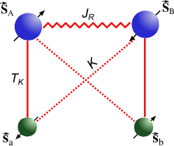
Figure 1: (color online) The cartoon picture of the RS model: the local magnetic moments and the conduction electron spins are denoted by big blue circled and small green circled arrows, respectively. $T_{K}$, $J_{R}$, and $K$ represent the single-ion Kondo energy scale, the RKKY interaction, and the interaction induced cross Kondo coupling. Various entanglements among these spins are defined in the text.

The eigenstates of $H_{RS}$ can be classified into six catalogs: two singlets, three triplets, and one quintet, according to the decomposition of tensor representations of the $SU(2)$ group: $\underline{\mathbf{2}}\otimes\underline{\mathbf{2}}\otimes\underline{\mathbf{2}}\otimes\underline{\mathbf{2}}=2\times\underline{\mathbf{1}}\oplus 3\times\underline{\mathbf{3}}\oplus\underline{\mathbf{5}}$ as listed in Appendix B. These eigenstates are constructed based on a complete set of the conventional basis $|S^{z}(A),s^{z}_{c}(a);S^{z}(B),s^{z}_{c}(b)\rangle$ and labeled by the total spin $S$, its z-component $S_{z}$, and the parity (with respect to permutations of the two local moments) Rasul . Because we consider $T_{K}$, $J_{R}$, and $K$ are all AFM, the groundstate is among the mixed states of the two singlets of even parity. They are denoted by (each up to a normalization factor)

$$|\Psi_{(0^{+})}\rangle = |\Downarrow\downarrow;\Uparrow\uparrow\rangle+|\Uparrow\uparrow;\Downarrow\downarrow\rangle$$

$$+ \frac{\Delta-J_{R}+2}{J_{R}-2K}(|\Downarrow\uparrow;\Downarrow\uparrow\rangle+|\Uparrow\downarrow;\Uparrow\downarrow\rangle)$$

$$+ \frac{-\Delta+2K-2}{J_{R}-2K}(|\Downarrow\uparrow;\Uparrow\downarrow\rangle+|\Uparrow\downarrow;\Downarrow\uparrow\rangle)$$

and

$$|\Psi_{(0^{\prime+})}\rangle = |\Downarrow\downarrow;\Uparrow\uparrow\rangle+|\Uparrow\uparrow;\Downarrow\downarrow\rangle$$

$$+ \frac{-\Delta-J_{R}+2}{J_{R}-2K}(|\Downarrow\uparrow;\Downarrow\uparrow\rangle+|\Uparrow\downarrow;\Uparrow\downarrow\rangle)$$

$$+ \frac{\Delta+2K-2}{J_{R}-2K}(|\Downarrow\uparrow;\Uparrow\downarrow\rangle+|\Uparrow\downarrow;\Downarrow\uparrow\rangle).$$

The corresponding eigen energies are

$$E_{(0^{+})} = E_{(0)}-\frac{1}{2}\Delta,$$ (4)

$$E^{\prime}_{(0^{+})} = E_{(0)}+\frac{1}{2}\Delta,$$ (5)

with $E_{(0)}=-J_{R}/4-K/2-1/2$ and $\Delta=\sqrt{(1+K-J_{R})^{2}+3(K-1)^{2}}$.

Another relevant low energy states are from the odd triplet

$$|\Psi_{(1^{-},+1)}\rangle = \frac{J_{R}+\sqrt{(K-1)^{2}+J_{R}^{2}}}{1-K}(|\Downarrow\uparrow;\Uparrow\uparrow\rangle-|\Uparrow\uparrow;\Downarrow\uparrow\rangle)$$

$$-|\Uparrow\downarrow;\Uparrow\uparrow\rangle+|\Uparrow\uparrow;\Uparrow\downarrow\rangle,$$

$$|\Psi_{(1^{-},~{}0)}\rangle = \frac{1-K+\sqrt{(K-1)^{2}+J_{R}^{2}}}{J_{R}}(|\Downarrow\uparrow;\Uparrow\downarrow\rangle-|\Uparrow\downarrow;\Downarrow\uparrow\rangle)$$

$$+|\Downarrow\downarrow;\Uparrow\uparrow\rangle-|\Uparrow\uparrow;\Downarrow\downarrow\rangle,$$

$$|\Psi_{(1^{-},-1)}\rangle = \frac{J_{R}+\sqrt{(K-1)^{2}+J_{R}^{2}}}{1-K}(|\Uparrow\downarrow;\Downarrow\downarrow\rangle-|\Downarrow\downarrow;\Uparrow\downarrow\rangle)$$ (6)

$$-|\Downarrow\uparrow;\Downarrow\downarrow\rangle+|\Downarrow\downarrow;\Downarrow\uparrow\rangle.$$

The corresponding eigen energy is

$$E_{(1^{-})}=-\frac{J_{R}}{4}-\frac{\sqrt{(K-1)^{2}+J_{R}^{2}}}{2}.$$ (7)

It is apparent that the groundstate of the RS Hamiltonian Eq.(1) is the singlet $|\Psi_{(0^{+})}\rangle$. However, the repulsive level spacing (energy gap) $\Delta$ vanishes at a special point $P$, corresponding to $K=T_{K}=J_{R}/2$, so that the singlet $|\Psi_{(0^{\prime+})}\rangle$ is degenerate with $|\Psi_{(0^{+})}\rangle$ at this point. Meanwhile, the odd triplet $|\Psi_{(1^{-})}\rangle$ is degenerate with $|\Psi_{(0^{+})}\rangle$ for $K=1,J_{R}\geq 2$. Hence the model indeed shows a strong frustration along the line $K=1$ and exhibits an enlarged symmetry at $P$note3 . The precise wavefunctions across the $P$ point can be determined by taking either limits ($K=1,J_{R}=2-\epsilon$) and ($K=1,J_{R}=2+\epsilon$), $\epsilon\rightarrow 0^{+}$. It readily reveals a discontinuity in $|\Psi_{(0^{+})}\rangle$ as shown in Appendix B.

III Entanglement phase diagram

Now, we start from the conventional Kondo impurity entanglement, i.e., the SIKE defined as the entanglement between a local moment, say ${\vec{S}}(A)$, and the rest of the system, denoted by $\tilde{A}$. It is measured by the van Norman entropy ${\cal E}_{SIKE}=-Tr_{(A)}\{\hat{\rho}_{imp}(A)\ln{\hat{\rho}}_{imp}(A)\}$, where ${\hat{\rho}}_{imp}(A)$ is the reduced density matrix ${\hat{\rho}}_{imp}(A)=Tr_{\tilde{A}}{\hat{\rho}}$. Here, ${\hat{\rho}}=|\Psi_{G}\rangle\langle\Psi_{G}|$ is the density matrix for the groundstate ( in our case $|\Psi_{G}\rangle=|\Psi_{(0^{+})}\rangle$) of the whole system. It is straightforwardly seen that ${\cal E}_{SIKE}=1$ due to the $SU(2)$-spin invariance, indicating a maximal entanglement between a local moment and the reminder of the whole system.

Next, we consider the TIKE, the entanglement of the two local moments with the conduction electrons. Following Ref.Cho , this entanglement is determined by the reduced density matrix of the two impurities, ${\hat{\rho}}_{imp}(AB)=Tr_{(c)}{\hat{\rho}}$, with $Tr_{(c)}$ indicating trace over the Hilbert subspace spanned by the conduction electrons. It can be quantified by the von Neumann entropyCho

$${\cal E}_{TIKE}=-p_{s}\log p_{s}-(1-p_{s})\log\frac{1-p_{s}}{3}.$$ (8)

Here, $p_{s}=\frac{1}{4}-f_{AB}$ is the fidelity of the spin singlet within the reduced two impurity state, and $f_{AB}=\langle{\Psi_{0^{+}}}|{\vec{S}}(A)\cdot{\vec{S}}(B)|{\Psi_{0^{+}}}\rangle$ is the spin-spin correlation function on the groundstate. In our case,

$$f_{AB}=\frac{1}{2}\frac{1+K-J_{R}}{\sqrt{(J_{R}-K-1)^{2}+3(K-1)^{2}}}-\frac{1}{4}.$$ (9)

${\cal E}_{TIKE}$ is then evaluated on the groundstate $|\Psi_{0^{+}}\rangle$ as shown in Fig.2. We find that ${\cal E}_{TIKE}$ is not only a smoothly varying function of $f_{AB}$ as already shown in Ref.Cho , but also a smooth function of $K$ and $J_{R}$ without detectable feature across the point $P$.

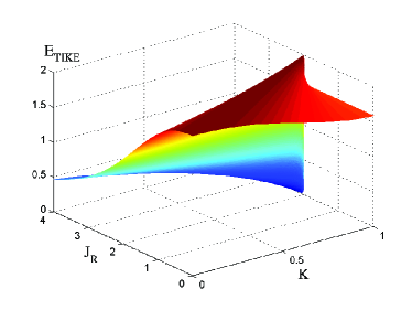
Figure 2: (color online) The TIKE as a function of $J_{R}$ and $K$.

Now we turn to the IIE. It can be measured by the concurrence or negativity , ${\cal C}_{IIE}$. Its evaluation is also related to the reduced two-impurity density matrix ${\hat{\rho}}_{imp}(AB)$. The concurrence can be expressed byCho

$${\cal C}_{IIE}=\max\{-2f_{AB}-1/2,0\}.$$ (10)

The result is plotted in Fig.3(a). For fixed $K<1$, ${\cal C}_{IIE}$ increases continuously with $J_{R}$. For $K=1$, ${\cal C}_{IIE}$ shows a sudden increase from zero to unity when $J_{R}$ goes across $J_{R}=2$.

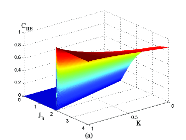
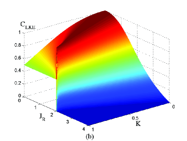
Figure 3: (color online) The concurrence of the IIE (a) and the LKE (b) as functions of $J_{R}$ and $K$. The single-ion Kondo energy scale is taken as unit $T_{K}=1$.

Together with the observed discontinuity in the groundstate wavefunction, the jump in IIE evidences a transition at $P$ Wu . But its relation with the suppression of Kondo effect remains uncertain. We now turn to an alternative definition of the Kondo entanglement, i.e., the LKE between a local moment, say ${\vec{S}}(A)$, and the conduction electron at its nearest neighbor site, ${\vec{s}}_{c}(a)$. The LKE differs to the conventional impurity entanglement as it involves only a spatially neighboring pair formed by a local moment and a conduction electron. This local Kondo pair is defined in the original real space point-contact Kondo interaction $J_{K}{\vec{S}_{A}}\cdot{\vec{s}_{c}(a)}$ (with $J_{K}$ being the original Kondo coupling) as shown in Appendix A. Similar to IIE, the LKE can be evaluated by the concurrence or negativity, via the corresponding reduced density matrix ${\hat{\rho}}_{LK}(Aa)=Tr_{({\tilde{A}}{\tilde{a}})}{\hat{\rho}}$, with $Tr_{({\tilde{A}}{\tilde{a}})}$ indicating the trace in the Hilbert space except the subspace spanned by ${\vec{S}}_{A}$ and ${\vec{s}}_{c}(a)$. Thus we have

$${\cal C}_{LKE}=\max\{-2f_{Aa}-1/2,0\},$$ (11)

where $f_{Aa}=\langle{\Psi_{0^{+}}}|{\vec{S}}(A)\cdot{\vec{s}}_{c}(a)|{\Psi_{0^{+}}}\rangle$ is the correlation function of the local Kondo singlet state,

$$f_{Aa}=\frac{1}{4}\frac{J_{R}+2K-4}{\sqrt{(J_{R}-K-1)^{2}+3(K-1)^{2}}}-\frac{1}{4}.$$ (12)

The result of ${\cal C}_{LKE}$ is plotted in Fig.3(b). Interestingly, ${\cal C}_{LKE}$ develops a maximum for $0<K<1$, $J_{R}<2$ and decreases monotonically for $J_{R}>2$. But along the line $K=1$ it shows a sudden suppression $J_{R}>2$ .

An entanglement phase diagram in terms of $K$ and $J_{R}$ is then drawn in Fig.4, where three different phases divided by the lines $J_{R}=K+1$ and $J_{R}=4-2K$ are indicated: the IIE phase (${\cal C}_{IIE}>0$,${\cal C}_{LKE}=0$), the LKE phase (${\cal C}_{LKE}>0$,${\cal C}_{IIE}=0$), and the co-existence phase (${\cal C}_{IIE}>0$, ${\cal C}_{LKE}>0$). The IIE and LKE phases contact only at the point $P$: by increasing $J_{R}$ across $P$ along the strong frustration line $K=1$, $f_{AB}$ has a sudden drop from $1/4$ to $-1/2$, $f_{Aa}$ has a jump from $-1/2$ to $0$. Or, ${\cal C}_{IIE}$ has a jump from $0$ to $1$ while ${\cal C}_{LKE}$ has a sudden drop from $1/2$ to $0$.

Therefore, together with the discontinuity of the wavefunction $|\Psi_{(0+)}\rangle$, the sudden changes along the line $K=1$ in the IIE and LKE do evidence a phase transition accompanied by a breakdown of Kondo effect. Of course, a true second order phase transition usually involves a continuous variation of the order parameter before its suppression. So the discontinuity exhibited in the IIE or LKE ( as an order parameter here) is seemingly due to the simplicity of the present model involving only two conduction electrons.

We notice that the inter-impurity spin-spin correlation function, closely related to the IIE discussed here, was actually calculated in the early numerical renormalization group study Jones88 at low yet finite temperatures, where the calculated quantity did not exhibit a sudden discontinuity but a rather sharp change at the critical point. Interestingly, a more recent calculation based on the natural orbitals renormlization group method does find a suddent jump of this quantity at zero tempertureHe15 . Therefore, the discontinuity of the IIE and LKE may be not limited to the present model, but a generic feature of the impurity state involving finite degrees of freedom at quantum critical points. This discontinuity could be smeared when the impurity degrees of freedom become infinite as in the Kondo lattice case.

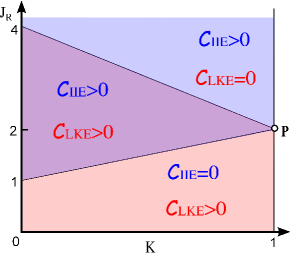
Figure 4: (color online) Entanglement phase diagram: there are three distinct phases divided by the lines ${\cal C}_{LKE}=0$ and ${\cal C}_{IIE}=0$. These two lines intersect at the singular point $P:(K=1,J_{R}=2)$, where the coexistence regime diminishes leading to a Kondo breakdown transition to the AFM singlet phase.

IV The fidelity of the Kondo and inter-impurity AFM singlets

In order to clarify whether the phase with non-zero ${\cal C}_{IIE}$ or ${\cal C}_{LKE}>0$ corresponds to the AFM inter-impurity or Kondo singlets, we calculate the normalized wavefunction overlaps $\langle\Psi_{AFM}|\Psi_{G}\rangle$ and $\langle\Psi_{KS}|\Psi_{G}\rangle$, respectively. We consider the pure state of the Kondo screening phase (denoted by $|\Psi_{KS}\rangle$) as the groundstate at the fixed point $K=J_{R}=0$. Similarly, we denote $|\Psi_{AFM}\rangle$ the pure inter-impurity AFM state at the fixed point $K=0,J_{R}\rightarrow\infty$. Here, $|\Psi_{KS}\rangle=|\Psi_{(0)Aa}\rangle\otimes|\Psi_{(0)Bb}\rangle$, $|\Psi_{AFM}\rangle=|\Psi_{(0)AB}\rangle\otimes|\Psi_{(0)ab}\rangle$, with $|\Psi_{(0)Aa}\rangle=\frac{1}{\sqrt{2}}(|\Uparrow\downarrow\rangle-|\Downarrow\uparrow\rangle)$, $|\Psi_{(0)Bb}\rangle=\frac{1}{\sqrt{2}}(|\Uparrow\downarrow\rangle-|\Downarrow\uparrow\rangle)$, $|\Psi_{(0)AB}\rangle=\frac{1}{\sqrt{2}}(|\Uparrow\Downarrow\rangle-|\Downarrow\Uparrow\rangle)$, $|\Psi_{(0)ab}\rangle=\frac{1}{\sqrt{2}}(|\uparrow\downarrow\rangle-|\downarrow\uparrow\rangle)$.

We find that in the regime with ${\cal C}_{IIE}=0$ or ${\cal C}_{LKE}=0$ the respective wavefunction overlap vanishes. Therefore, the obtained entanglement phase diagram Fig.4 reflects the overall evolution from the Kondo singlet to the inter-impurity AFM singlet.

Specifically, increasing $K$ will enhance the frustration, so that the fidelities of $|\Psi_{KS}\rangle$ and $|\Psi_{AFM}\rangle$ on the true groundstate $|\Psi_{G}\rangle$ change with varying $J_{R}$. The fidelities can be calculated as the normalized wavefunction overlaps $\langle\Psi_{G}|\Psi_{AFM}\rangle$ and $\langle\Psi_{G}|\Psi_{KS}\rangle$. The three-dimensional plots of the wavefunctions overlaps are shown in Fig.5(a) and Fig. 5(b), respectively. Fig.6(a) and Fig.6(b) show the $J_{R}$-dependence of these quantities for fixed values of $K$. We find that $\langle\Psi_{G}|\Psi_{AFM}\rangle$ increases rapidly with $J_{R}$ and saturates to 1 after entering the AFM phase, $J_{R}>2$. Notice that $\langle\Psi_{G}|\Psi_{KS}\rangle$ always approaches to $1/2$ for $J_{R}\rightarrow\infty$, indicating that the Kondo singlet fidelity $p_{s}\rightarrow 1/2$. As shown in Appendix A, this implies the non-correlated Kondo state or a full suppression of Kondo effect.

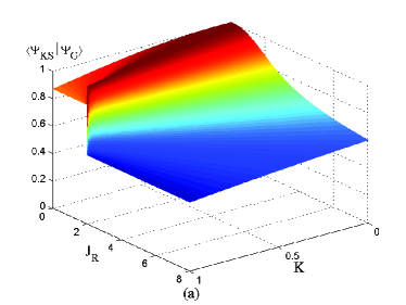
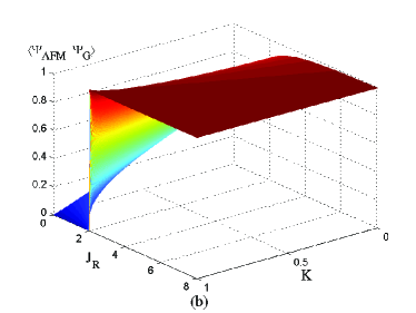
Figure 5: (color online) (a) The fidelity of the Kondo singlet $|\Psi_{KS}\rangle$ on the groundstate $|\Psi_{G}\rangle$. (b) The fidelity of the inter-impurity AFM singlet $|\Psi_{AFM}\rangle$ on the groundstate $|\Psi_{G}\rangle$.

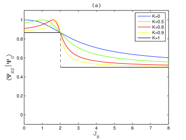
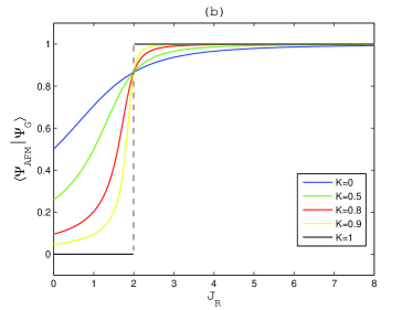
Figure 6: (color online) The groundstate fidelity of the Kondo singlet $|\Psi_{KS}\rangle$ (a) or of the inter-impurity AFM singlet (b) as a function of the RKKY interaction for various fixed frustration $K$.

V Entanglement sum rule

By definition, the concurrences of LKE and IIE introduced in the main text, ${\cal C}_{IIE}$ and ${\cal C}_{LKE}$, are always non-zero ( but $\leq 1$) when the respective correlation function $f_{AB}\leq-1/4$ or $f_{Aa}\leq-1/4$. Based on the exact solutions, these functions can be reexpressed as

$$f_{AB}=-\frac{\lambda}{2}\cos\theta-\frac{1}{4};f_{Aa}=\frac{\lambda}{4}\cos\theta-\frac{\sqrt{3}}{4}\sin\theta-\frac{1}{4}.$$ (13)

Where, $\theta=\tan^{-1}\frac{{\sqrt{3}}(1-K)}{|J_{R}-K-1|}$, $\lambda=\frac{J_{R}-K-1}{|J_{R}-K-1|}$. Therefore, in the whole parameter regime $J_{R}\geq 0$, $K\leq 1$, or $0\leq\theta\leq\frac{\pi}{2}$, we have

$${\cal C}_{IIE} = \max\{\lambda\cos\theta,0\};$$ (14)

$${\cal C}_{LKE} = \max\{-\frac{\lambda}{2}\cos\theta+\frac{\sqrt{3}}{2}\sin\theta,0\}.$$ (15)

Thus ${\cal C}_{IIE}$ and ${\cal C}_{LKE}$ are both non-zero when $K+1<J_{R}<4-2K$. In this co-existence regime where $\frac{\pi}{6}<\theta<\frac{\pi}{2}$, we have

$${\cal C}_{IIE}+{\cal C}_{LKE}=\sin(\theta+\frac{\pi}{6}).$$ (16)

This is a sum rule constraining the variations of ${\cal C}_{IIE}$ and ${\cal C}_{LKE}$: $\frac{\sqrt{3}}{2}<{\cal C}_{IIE}+{\cal C}_{LKE}<1$ in this regime.

As an inference of the sum rule, we note that a Werner state with $p_{s}\geqq(1+3/\sqrt{2})/4\approx 0.78$ has the nonlocal correlation characteristic, i.e., violation of the Bell inequalityCho ; Clauser ; Horodecki . This value corresponds to ${\cal C}\geqq 0.56$. Therefore, we have an entanglement monogamy: ${\cal C}_{LKE}$ and ${\cal C}_{IIE}$ cannot simultaneously maximize, nor even simultaneously fall into this region. In other words, only one of the entanglements could be maximized or violate the Bell inequality.

Finally, one can also define the entanglement between the spin ${\vec{S}}_{A}$ and ${\vec{s}}_{c}(b)$, i.e., the cross Kondo entanglement, quantified by ${\cal C}_{CKE}$. Owing to the discrete symmetry mentioned previously, this quantity can be drived similar to ${\cal C}_{LKE}$, obtaining ${\cal C}_{CKE}=\max\{-\frac{\lambda}{2}\cos\theta-\frac{\sqrt{3}}{2}\sin\theta,0\}$. So ${\cal C}_{CKE}$ is non-zero only when $J_{R}<4K-2$. This region is a subregion of the LKE phase, below the straight line connecting ($K=0.5,J_{R}=0$) and the $P$-point(not shown in Fig.4 ). Hence including ${\cal C}_{CKE}$ does not violate the previous sum rule. Moreover, another sum rule ${\cal C}_{LKE}+{\cal C}_{CKE}=\cos\theta$ holds in this subregion. Therefore the previous inference as well as all the conclusions in the main text remain valid in the whole phase diagram.

VI Implications and discussions

As we emphasized, the quantum entanglement related to the single-ion Kondo effect is complicated when two or more local magnetic impurities are introduced. We have considered the LKE in the case of two magnetic impurities where a quantum phase transition from the Kondo to the AFM singlets takes place. The exact results obtained from a simplified yet effective TIKM, i.e., the RS spin model, show a phase diagram involving several regimes corresponding to non zero LKE and IIE, and their co-existence. With increasing frustrated cross coupling the co-existence regime shrinks and vanishes at the critical point $P$ where the groundstate $|\Psi_{G}\rangle$ has a discontinuity accompanied by jumps in the IIE and LKE. The discontinuity of such quantities at the critical point may be a generic feature caused by the non-extensive impurity term in the free energy of the TIKMBayat14 ; He15 .

Due to the entanglement sum rule, the LKE and IIE cannot be simultaneously maximized even in the co-existence regime. Because an entangled state with non-zero concurrence while still keeping the Bell-CHSH inequalityClauser ; Horodecki can be used for quantum information processing including quantum teleportationPopescu ; Lee , the singlet groundstate in the co-existence phase shares this feature either by the LKE or IIE, and thus should be an interesting candidate state for quantum information processing.

It is interesting to understand implications of our present study for more generic Kondo lattice models. In these systems, like the heavy fermion metals, the magnetic quantum phase transitions may be influenced by the variation of Kondo effect. A local quantum phase transition is possible in more generic Kondo lattice phase diagram where the criticality is associated with a critical breakdown of the single-ion Kondo effectSi2 ; Coleman2 ; Si3 . Near the critical point, the Hall constant shows a discontinuous jump due to the reconstruction of the Fermi surface across the critical pointSi2 ; Coleman2 . Experimental evidence for this scenario comes from several prototypes of heavy fermion metals including YbRh₂Si₂Paschen04 and CeNiAsOLuo where the observed Hall constant exhibits a sudden change accompanying the magnetic phase transition.

Although the above scenario could be naturally understood based on the Kondo entanglement picture, a lattice model Hamiltonian with exact solutions showing the Kondo entanglement breakdown transition is lacking. Thus our studied model can serve as a toy model to understand its basic physics from the quantum entanglement perspective. On the one hand, one expects that with the evolution from two impurities to an regular local moment lattice, the Kondo singlet and inter-impurity AFM singlet states evolve into the paramagnetic heavy fermion and AFM ordered phases, respectively. On the other hand, in addition to the RKKY interaction, the crossing Kondo coupling ($K$) emerges as a many-body frustration effect and plays a role in controlling the transition. Generally, in the regime with relatively small $K$, the Kondo and inter-impurity singlets can co-exist in the intermediate regime of $J_{R}$. The co-existence regime diminishes with increasing $K$ and a direct Kondo singlet breakdown transition takes place when the Kondo coupling is maximally frustrated (at $K=T_{K}$). In the Kondo lattice phase diagram this condition should correspond to the regime with strong geometric frustrations and quantum fluctuations but no spin liquid phase sets inSi3 . Finally, extending the present study to the Kondo lattice cases with frustrated cross couplings or various anisotropic interactions is not an easy task but highly desirable. Nevertheless, our present result already provides a concrete example of Kondo breakdown quantum phase transition from the quantum entanglement perspective.

Appendix A The LKE in the $N$-impurity Kondo system

The Kondo system consisting of a metallic electron host, with energy dispersion $\epsilon({\vec{k}})$, and $N$-number of quantum mechanical magnetic moments (of spin-1/2) localized at sites $i$, $i=1,2,......,N$, is described by the Hamiltonian

$$H_{NKM} = \sum_{\sigma=\uparrow,\downarrow}\int d^{3}{\vec{k}}~{}\epsilon({\vec{k}})c^{\dagger}_{\sigma}({\vec{k}})c_{\sigma}({\vec{k}})$$ (17)

$$+J_{K}\sum^{N}_{i=1}{\vec{S}}_{i}\cdot{\vec{s}}_{c}({\vec{r}}_{i}),$$

where the Kondo coupling is either antiferromagnetic ($J_{K}>0$) and local, in the sense that it takes place between a local moment ${\vec{S}}_{i}$ and a spatially nearby conduction electron at site ${\vec{r}}_{i}$ via the point-like interaction $J_{K}{\vec{S}}_{i}\cdot{\vec{s}}_{c}({\vec{r}}_{i})$, with the electron spin operator ${\vec{s}}_{c}({\vec{r}}_{i})=\frac{1}{2}c^{\dagger}_{\sigma}({\vec{r}}_{i}){\vec{\sigma}}_{\sigma\sigma^{\prime}}c_{\sigma^{\prime}}({\vec{r}}_{i})$.

The local Kondo entanglement (LKE) refers to the quantum entanglement of a local Kondo pair consisting of an impurity fixed spin ${\vec{S}}_{i}$ and its spatially nearby conduction electron. As we focus on the spin degrees of freedom relevant in the Kondo screening, such a pair of spins is dubbed as a local Kondo state. It constitutes a subsystem, with a local Hilbert space $\Omega_{i}$ spanned by ${\vec{S}}_{i}$ and ${\vec{s}}_{c}({\vec{r}}_{i})$. Let $\Omega$ be the total Hilbert space, and ${\tilde{\Omega}_{i}}$ the Hilbert subspace complementary to $\Omega_{i}$: $\Omega_{i}\cup{\tilde{\Omega}_{i}}=\Omega$. Assume $|\Psi_{G}\rangle$ be the groundstate of the $N$-impurity Kondo model $H_{NKM}$ defined in Eq.(17), ${\hat{\rho}}=|\Psi_{G}\rangle\langle\Psi_{G}|$ the corresponding density matrix of the whole system, the LKE is defined as the entanglement of the reduced density matrix of this subsystem obtained by taking trace over all other degrees of freedom except the local Hilbert space: ${\hat{\rho}}_{\Omega_{i}}=Tr_{{\tilde{\Omega}}_{i}}{\hat{\rho}}$. Obviously, $\Omega_{i}$ has dimension 4, so ${\hat{\rho}}_{\Omega_{i}}$ can be expressed by the matrices $I_{4\times 4}$, ${\vec{\tau}}\otimes{\vec{\sigma}}$, with ${\vec{\tau}}$ being the Pauli matrices of the local spin, ${\vec{S}}_{i}=\frac{1}{2}{\vec{\tau}}_{i}$Nielson . Owing to the fact that the Hamiltonian is real, $SU(2)$ invariant, and the groundstate is always a spin-singlet, one has the general formNielson ; Amico

$${\hat{\rho}}_{\Omega_{i}}=\frac{1}{4}I_{4\times 4}+\frac{r}{4}[{\tau^{x}_{i}\otimes\sigma^{x}_{i}}+{\tau^{y}_{i}\otimes\sigma^{y}_{i}}+{\tau^{z}_{i}\otimes\sigma^{z}_{i}}].$$ (18)

In terms of the Bell basis, the maximal entangled states $|\Psi^{(\pm)}\rangle=\frac{1}{\sqrt{2}}(|\Uparrow\downarrow\rangle\pm|\Downarrow\uparrow\rangle)$ and $|\Phi^{(\pm)}\rangle=\frac{1}{\sqrt{2}}(|\Uparrow\uparrow\rangle\pm|\Downarrow\downarrow\rangle)$, the reduced density matrix can be expressed by

$${\hat{\rho}}_{\Omega_{i}} = p_{s}|\Psi^{(-)}\rangle\langle\Psi^{(-)}|$$

$$+ p_{t}(|\Psi^{(+)}\rangle\langle\Psi^{(+)}|+|\Phi^{(+)}\rangle\langle\Phi^{(+)}|+|\Phi^{(-)}\rangle\langle\Phi^{(-)}|),$$

with $p_{s}$ and $p_{t}$ being the probabilities of spin singlet and spin-triplet, respectively. Thus, ${\hat{\rho}}_{\Omega_{i}}$ is a mixture of spin-singlet and spin-triplet. $p_{s}$ and $p_{t}$ are related to the spin-spin correlation function $f_{s}=\langle\Psi_{G}|{\vec{S}}_{i}\cdot{\vec{s}}({\vec{r}}_{i})|\Psi_{G}\rangle$ via $p_{s}=\frac{1}{4}-f_{s}$,$p_{t}=\frac{1}{4}+\frac{f_{s}}{3}$. Therefore, the pure local Kondo singlet corresponds to $p_{s}=1$ or $f_{s}=-\frac{3}{4}$, while the pure local Kondo triplet corresponds to $p_{t}=\frac{1}{3}$ or $f_{s}=\frac{1}{4}$. Notice that the case of $f_{s}=-\frac{1}{4}$ or $p_{s}=p_{t}=1/2$ corresponds to the non-correlated Kondo pair with equal mixture of spin-singlet and spin triplet.

In our definition, the LKE is measured by the concurrence of ${\hat{\rho}}_{\Omega_{i}}$. Because ${\hat{\rho}}_{\Omega_{i}}$ can be reexpressed as ${\hat{\rho}}_{\Omega_{i}}=\frac{4p_{s}-1}{3}|\Psi^{(-)}\rangle\langle\Psi^{(-)}|+\frac{1-p_{t}}{3}I_{4\times 4}$, it is also a Werner stateWerner with the spin singlet fidelity $p_{s}=\langle\Psi^{(-)}|{\hat{\rho}}_{\Omega_{i}}|\Psi^{(-)}\rangle$. The the concurrence of this state is given byWootters

$${\cal C}_{LKE}=\max\{2p_{s}-1,0\}.$$ (20)

Such entanglement can be also measured by the negativityVidal of the reduced density matrix, ${\cal N}_{{\hat{\rho}}_{\Omega_{i}}}$. It is straightforwardly seen that the negativity of the Werner state is equal to the concurrenceLee , i.e., ${\cal N}_{{\hat{\rho}}_{\Omega_{i}}}={\cal C}_{LKE}$.

Similarly, the entanglement of a pair of two local magnetic moments, say ${\vec{S}}_{i}$ and ${\vec{S}}_{j}$, can be defined following the previous approach. Parallel to the LKE, such the inter-impurity entanglement (IIE) measured by the concurrence (${\cal C}_{IIE}$) is closely related to the spin-spin correlation function $\langle\Psi_{G}|{\vec{S}}_{i}\cdot{\vec{S}}_{j}|\Psi_{G}\rangle$. This quantity varies monotonically with the RKKY interaction $J_{R}(ij)$. The indirect RKKY interaction, i.e., the coupling between the local moments which is not explicitly present in the bare Hamiltonian, is generated in the second order perturbtion in $J_{K}$ and dependend on the density of states at the Fermi energy and the spatial separation $|{\vec{R}}_{i}-{\vec{R}}_{j}|$ of the two local moments. Because $J_{R}(ij)$ oscillates non-universally, the IIE’s of different pairs $(i,j)$ are usually complicated. Remarkably, there are two special situations where the IIE competes with the LKE: (i) the two impurity case with $N=2$; (ii) The sites $i$ and $j$ are the nearest-neighboring sites in the Kondo lattice with $N=L$ ($L=$ the total number of sites). Therefore, the competition between the LKE and IIE manifests the competition between the Kondo singlet and the inter-impurity AFM singlet in the TIKM, or manifests the competition between the paramagnetic heavy Fermion state and the AFM ordered state in the Kondo lattices.

A phenomenological understanding of above competition invokes two energy scales, the single-ion Kondo temperature $T_{K}\sim D\sqrt{\rho_{F}J_{K}}\exp[-\frac{1}{\rho_{F}J_{K}}]$, and the RKKY interaction $J_{R}$, with $D$ the band width and $\rho_{F}$ the density of states at the Fermi energy. In the renormalization group treatment one approaches the low energy limit by gradually integrating out the degrees of freedom of conduction electrons. So that at $T=0$, the latter can be introduced by adding a direct RKKY term $J_{R}{\vec{S}}_{i}\cdot{\vec{S}}_{j}$ into the original Hamiltonian, while the single-ion Kondo screening effect is described by a term $T_{K}{\vec{S}}_{i}\cdot{\vec{s}}_{c}({\vec{r}}_{i})$. Phenomenologically, $T_{K}$ is the excitation energy of the Kondo triplet above the Kondo singlet groundstate. The effective cross Kondo coupling (denoted by $K$ in the main text) between ${\vec{S}}_{j}$ and ${\vec{s}}_{c}({\vec{r}}_{i})$ can be also induced by pure quantum mechanical many-body processes. Proper inter-impurity distance and the direct RKKY interaction guarantee the required particle-hole symmetryAffleck2 . These interpretations provide a basis for the RS spin model as a minimal fixed point Hamiltonian of the TIKM.

Appendix B Eigenstates and eigen energies of the Rasul-Schlottmann model

The sixteen eigenstates (each up to a normalization factor) and the corresponding eigenvalues are solved as following:

$$|\Psi_{(0^{+})}\rangle = |\Downarrow\downarrow;\Uparrow\uparrow\rangle+|\Uparrow\uparrow;\Downarrow\downarrow\rangle+c_{1}(|\Downarrow\uparrow;\Downarrow\uparrow\rangle+|\Uparrow\downarrow;\Uparrow\downarrow\rangle)$$ (21)

$$-(c_{1}+1)(|\Downarrow\uparrow;\Uparrow\downarrow\rangle+|\Uparrow\downarrow;\Downarrow\uparrow\rangle)$$

$$E_{(0^{+})} = -\frac{J_{R}}{4}-\frac{K}{2}-\frac{1}{2}$$ (22)

$$-\frac{\sqrt{(1+K-J_{R})^{2}+3(K-1)^{2}}}{2}$$

$$|\Psi_{(0^{\prime+})}\rangle = |\Downarrow\downarrow;\Uparrow\uparrow\rangle+|\Uparrow\uparrow;\Downarrow\downarrow\rangle+c_{2}(|\Downarrow\uparrow;\Downarrow\uparrow\rangle+|\Uparrow\downarrow;\Uparrow\downarrow\rangle)$$ (23)

$$-(c_{2}+1)(|\Downarrow\uparrow;\Uparrow\downarrow\rangle+|\Uparrow\downarrow;\Downarrow\uparrow\rangle)$$

$$E_{(0^{\prime+})} = -\frac{J_{R}}{4}-\frac{K}{2}$$ (24)

$$-\frac{1}{2}+\frac{\sqrt{(1+K-J_{R})^{2}+3(K-1)^{2}}}{2}$$

$$|\Psi_{(1^{+},+1)}\rangle = |\Downarrow\uparrow;\Uparrow\uparrow\rangle-|\Uparrow\downarrow;\Uparrow\uparrow\rangle+|\Uparrow\uparrow;\Downarrow\uparrow\rangle-|\Uparrow\uparrow;\Uparrow\downarrow\rangle$$

$$|\Psi_{(1^{+},~{}0)}\rangle = |\Downarrow\uparrow;\Downarrow\uparrow\rangle-|\Uparrow\downarrow;\Uparrow\downarrow\rangle$$ (25)

$$|\Psi_{(1^{+},-1)}\rangle = |\Uparrow\downarrow;\Downarrow\downarrow\rangle-|\Downarrow\uparrow;\Downarrow\downarrow\rangle+|\Downarrow\downarrow;\Uparrow\downarrow\rangle-|\Downarrow\downarrow;\Downarrow\uparrow\rangle$$

$$E_{(1^{+})}=\frac{J_{R}}{4}-\frac{K}{2}-\frac{1}{2}$$ (26)

$$|\Psi_{(1^{-},+1)}\rangle = c_{3}(|\Downarrow\uparrow;\Uparrow\uparrow\rangle-|\Uparrow\uparrow;\Downarrow\uparrow\rangle)$$

$$-|\Uparrow\downarrow;\Uparrow\uparrow\rangle+|\Uparrow\uparrow;\Uparrow\downarrow\rangle$$

$$|\Psi_{(1^{-},~{}0)}\rangle = |\Downarrow\downarrow;\Uparrow\uparrow\rangle-|\Uparrow\uparrow;\Downarrow\downarrow\rangle$$ (27)

$$+c_{4}(|\Downarrow\uparrow;\Uparrow\downarrow\rangle-|\Uparrow\downarrow;\Downarrow\uparrow\rangle)$$

$$|\Psi_{(1^{-},-1)}\rangle = c_{3}(|\Uparrow\downarrow;\Downarrow\downarrow\rangle-|\Downarrow\downarrow;\Uparrow\downarrow\rangle)$$

$$-|\Downarrow\uparrow;\Downarrow\downarrow\rangle+|\Downarrow\downarrow;\Downarrow\uparrow\rangle$$

$$E_{(1^{-})}=-\frac{J_{R}}{4}-\frac{\sqrt{(K-1)^{2}+J_{R}^{2}}}{2}$$ (28)

$$|\Psi_{(1^{\prime-},+1)}\rangle = c_{5}(|\Downarrow\uparrow;\Uparrow\uparrow\rangle-|\Uparrow\uparrow;\Downarrow\uparrow\rangle)$$

$$-|\Uparrow\downarrow;\Uparrow\uparrow\rangle+|\Uparrow\uparrow;\Uparrow\downarrow\rangle$$

$$|\Psi_{(1^{\prime-},~{}0)}\rangle = |\Downarrow\downarrow;\Uparrow\uparrow\rangle-|\Uparrow\uparrow;\Downarrow\downarrow\rangle$$ (29)

$$+c_{6}(|\Downarrow\uparrow;\Uparrow\downarrow\rangle-|\Uparrow\downarrow;\Downarrow\uparrow\rangle)$$

$$|\Psi_{(1^{\prime-},-1)}\rangle = c_{5}(|\Uparrow\downarrow;\Downarrow\downarrow\rangle-|\Downarrow\downarrow;\Uparrow\downarrow\rangle)$$

$$-|\Downarrow\uparrow;\Downarrow\downarrow\rangle+|\Downarrow\downarrow;\Downarrow\uparrow\rangle$$

$$E_{(1^{\prime-})}=-\frac{J_{R}}{4}+\frac{\sqrt{(K-1)^{2}+J_{R}^{2}}}{2}$$ (30)

$$|\Psi_{(2,~{}2)}\rangle = |\Uparrow\uparrow;\Uparrow\uparrow\rangle$$

$$|\Psi_{(2,~{}1)}\rangle = |\Downarrow\uparrow;\Uparrow\uparrow\rangle+|\Uparrow\downarrow;\Uparrow\uparrow\rangle+|\Uparrow\uparrow;\Downarrow\uparrow\rangle+|\Uparrow\uparrow;\Uparrow\downarrow\rangle$$

$$|\Psi_{(2,~{}0)}\rangle = |\Downarrow\downarrow;\Uparrow\uparrow\rangle+|\Downarrow\uparrow;\Downarrow\uparrow\rangle+|\Downarrow\uparrow;\Uparrow\downarrow\rangle+|\Uparrow\downarrow;\Downarrow\uparrow\rangle$$ (31)

$$+|\Uparrow\downarrow;\Uparrow\downarrow\rangle+|\Uparrow\uparrow;\Downarrow\downarrow\rangle$$

$$|\Psi_{(2,-1)}\rangle = |\Uparrow\downarrow;\Downarrow\downarrow\rangle+|\Downarrow\uparrow;\Downarrow\downarrow\rangle+|\Downarrow\downarrow;\Uparrow\downarrow\rangle+|\Downarrow\downarrow;\Downarrow\uparrow\rangle$$

$$|\Psi_{(2,-2)}\rangle = |\Downarrow\downarrow;\Downarrow\downarrow\rangle$$

$$E_{(2^{+})}=\frac{J_{R}}{4}+\frac{K}{2}+\frac{1}{2}$$ (32)

In above, $c_{1}=\frac{\sqrt{(1+K-J_{R})^{2}+3(K-1)^{2}}-J_{R}+2}{J_{R}-2K}$, $c_{2}=\frac{-\sqrt{(1+K-J_{R})^{2}+3(K-1)^{2}}-J_{R}+2}{J_{R}-2K}$, $c_{3}=\frac{J_{R}+\sqrt{(K-1)^{2}+J_{R}^{2}}}{1-K}$, $c_{4}=\frac{1-K+\sqrt{(K-1)^{2}+J_{R}^{2}}}{J_{R}}$, $c_{5}=\frac{J_{R}-\sqrt{(K-1)^{2}+J_{R}^{2}}}{1-K}$, and $c_{6}=\frac{1-K-\sqrt{(K-1)^{2}+J_{R}^{2}}}{J_{R}}$. Along the line $K=1$ or $J_{R}=2K$, some coefficients are divergent, but the correct forms can be obtained by taking the limits from either sides. In particular, in the vicinity of the singular point $P:(K=1,J_{R}=2)$, the wavefunctions are determined unambiguously by taking the limits at $P$ approached from either sides along the line $K=1$. For instance, when $K=1$, $J_{R}=2+\epsilon$, $\epsilon\rightarrow 0^{+}$, we have the normalized state

$$|\Psi_{(0^{+})}\rangle_{+} = \frac{1}{2}[-|\Uparrow\uparrow;\Downarrow\downarrow\rangle-|\Downarrow\downarrow;\Uparrow\uparrow\rangle$$ (33)

$$+|\Downarrow\uparrow;\Uparrow\downarrow\rangle+|\Uparrow\downarrow;\Downarrow\uparrow\rangle].$$

While when $K=1$, $J_{R}=2-\epsilon$, $\epsilon\rightarrow 0^{+}$, we have

$$|\Psi_{(0^{+})}\rangle_{-} = \frac{1}{2{\sqrt{3}}}[2|\Uparrow\downarrow;\Uparrow\downarrow\rangle+2|\Downarrow\uparrow;\Downarrow\uparrow\rangle-|\Uparrow\uparrow;\Downarrow\downarrow\rangle$$ (34)

$$-|\Downarrow\downarrow;\Uparrow\uparrow\rangle-|\Downarrow\uparrow;\Uparrow\downarrow\rangle-|\Uparrow\downarrow;\Downarrow\uparrow\rangle].$$

Therefore, ${}_{+}\langle\Psi_{(0^{+})}|\Psi_{(0^{+})}\rangle_{-}=0$. This result demonstrates a discontinuity of the groundstate wavefunction across the singular point.

References

- (1) A. Osterloh, L. Amico, G. Falci, and R. Fazio, Nature 416, 608 (2002).
- (2) T.J. Osborne and M.A. Nielson, Phys. Rev. A 66, 032110 (2002).
- (3) G. Vidal, J.I. Latorre, E. Rico, and A. Kitaev, Phys. Rev. Lett. 90, 227902 (2003).
- (4) L. Amico, R. Fazio, A. Osterloh, and V. Vedral, Rev. Mod. Phys. 80, 517 (2008).
- (5) R. Horodecki, P. Horodecki, M. Horodecki, and K. Horodecki, Rev. Mod. Phys. 81, 865 (2009).
- (6) A.C. Hewson, The Kondo Problem to Heavy Fermions, Cambridge University Press, Cambridge, England, 1993.
- (7) P. Coleman, in Handbook of Magnetism and Advanced Magnetic Materials, V.1, 95 (Wiley, 2007).
- (8) C. Jayaprakash, H.R. Krishnamurthy, and J.W. Wilkins, Phys. Rev. Lett. 47, 737(1981).
- (9) B.A. Jones and C.M. Varma, Phys. Rev. Lett. 58, 843 (1987); B.A. Jones, C.M. Varma, and J.W. Wilkins, Phys. Rev. Lett. 61, 125 (1988).
- (10) S. Doniach, Physica B+C 91, 231 (1977).
- (11) L.I. Glazman and R.C. Ashoori, Science 304, 524 (2004).
- (12) N.J. Craig et al., Science 304, 565(2004).
- (13) P. Gegenwart, Q. Si, and F. Steglich, Nature Phys. 4, 186 (2008).
- (14) B.A. Jones and C.M. Varma, Phys. Rev. B 40, 324 (1989); B.A. Jones, B.G. Kotliar, and A.J. Millis, Phys. Rev. B 39, 3415 (1989).
- (15) I. Affleck and A.W.W. Ludwig, Phys. Rev. Lett. 68, 1046 (1992)
- (16) J.W. Rasul and P. Schlottmann, Phys. Rev. Lett. 62, 1701 (1989); P. Schlottmann and J.W. Rasul, Physica B 163, 544 (1990).
- (17) I. Affleck, A.W.W. Ludwig, and B.A. Jones, Phys. Rev. B 52, 9528 (1995).
- (18) O. Sakai, Y. Shimizu, and T. Kasuya, Solid State Commun. 75, 81 (1990).
- (19) R.M. Fye, Phys. Rev. Lett. 72, 916 (1994).
- (20) J. Gan, Phys. Rev. Lett. 74, 2583 (1995).
- (21) J.B. Silva et al., Phys. Rev. Lett. 76, 275 (1996).
- (22) G. Zarand, C.H. Chung, P. Simon, and M. Vojta, Phys. Rev. Lett. 97, 166802 (2006).
- (23) There are two types of particle-hole symmetry in the TIKM with lattice inversion symmetry, depending on the inter-impurity distance being even or odd lattice spacing, respectively. Usually, only the first type with even inter-impurity distance is the required symmetry which may guarantee a critical point with groundstate degeneracyJones89 ; Affleck2 . As an effective spin-only model, Eq.(1) does not show such distinction for even/odd inter-impurity distance. Instead, the required groundstate degeneracy can arise by tuning the cross Kondo coupling, see the following discussions.
- (24) A.T. Costa, Jr. and S. Bose, Phys. Rev. Lett. 87, 277901 (2001).
- (25) K. Le Hur, P. Doucet-Beaupre, and W. Hofstetter, Phys. Rev. Lett. 99, 126801 (2007).
- (26) K. Le Hur, Ann. Phys. 323, 2008 (2008).
- (27) I. Affleck, N. Laflorencie, and E.S. Sorensen, J. Phys. A 42, 504009 (2009).
- (28) A.T. Costa, Jr., S. Bose, and Y. Omar, Phys. Rev. Lett. 96, 230501 (2006).
- (29) S.Y. Cho and R.H. Mckanzie, Phys. Rev. A 73, 012109 (2006).
- (30) E. Eriksson and H. Jonhannesson, Phys. Rev. B 84, 041107(R) (2011).
- (31) H. Saleur, P. Schmitteckert, and R. Vasseur, Phys. Rev. B 88, 085413 (2013).
- (32) K. Yosida, Phys. Rev. 147, 223 (1966).
- (33) C.H. Bennetti, Phys. Rev. A 54, 3824 (1996).
- (34) A. Bayat, S. Bose, P. Sodano, and H. Johannesson, Phys. Rev. Lett. 109, 066403 (2012).
- (35) W.K. Wootters, Phys. Rev. Lett. 80, 2245 (1998).
- (36) G. Vidal and R.F. Werner, Phys. Rev. A 65, 032314 (2002).
- (37) M.-F. Yang, Phys. Rev. A 71, 030302(R)(2005).
- (38) The discontinuity in the first derivative of negativity usually comes from the requirement of nonnegative concurrenceYang . Its relation with a true quantum phase transition should be further corroborated by checking the nonanalyticity of groundstate energy or groundstate wavefunction.
- (39) In some circumstances such as in psudo-gaped or dissipative hosts the SIKE measured by the von Neumann entropy can show a peak feature at the quantum critical pointsHur1 ; Hur2 .
- (40) In a spin chain model with two magnetic impurites several impurity-related entanglement quantities measured by the negativity display detectable features in their derivatives at the quantum phase transition Bayat . These quantities do not exhibit apparant variation of the Kondo effect across the transition. More recently, the Schmidt gap has been proposed as an order parameter measuring the impurity quantum phase transitionsBayat14 .
- (41) A. Bayat, H. Johannesson, S. Bose, and P. Sodano, Nat. Commun. 5, 3784 (2014).
- (42) In the conformal field theory and non-Abelian bosonization approaches the enlarged hidden symmetry at the non-trivial critical point is identifiedAffleck2 ; Gan .
- (43) L.-A. Wu, M.S. Sarandy, and D.A. Lidar, Phys. Rev. Lett. 93, 250404 (2004).
- (44) R.-Q. He, J. Dai, and Z.-Y. Lu, arXiv:1501.01834, 2015.
- (45) J.F. Clauser, M.A. Horne, A. Shimony, and R.A. Holt, Phys. Rev. Lett. 23, 880 (1969).
- (46) R. Horodecki, P. Horodecki, and M. Horodecki, Phys. Lett. A 200, 340 (1995).
- (47) S. Popescu, Phys. Rev. Lett. 72, 797 (1994).
- (48) J. Lee and M.S. Kim, Phys. Rev. Lett. 84, 4236 (2000).
- (49) Q. Si, S. Rabello, K. Ingersent, and J.L. Smith, Nature 413, 804 (2001).
- (50) P. Coleman, C. Pepin, Q. Si and R. Ramazashvili, J. Phys. C 13, R723 (2001).
- (51) Q. Si, Physica B: Conden. Mat. 378, 23 (2006).
- (52) S. Paschen et al., Nature 432, 881 (2004).
- (53) Y.K. Luo et al., Nature Materials13, 777 (2014).
- (54) M. Nielson and I. Chuang, Quantum Computation and Quantum Information (Cambridge University Press, Cambridge, 2000).
- (55) R.F. Werner, Phys. Rev. A 40, 4277 (1989).
- (56) S. Lee, D.P. Chi, S.D. Oh, and J. Kim, Phys. Rev. A 68, 062304 (2003).