A Deep XMM-Newton Survey of M33: Point Source Catalog, Source Detection and Characterization of Overlapping Fields

Abstract

We have obtained a deep 8-field XMM-Newton mosaic of M33 covering the galaxy out to the D₂₅ isophote and beyond to a limiting 0.2–4.5 keV unabsorbed flux of 5$\times$10^-16 erg cm^-2 s^-1 (L${>}$4$\times$10³⁴ erg s^-1 at the distance of M33). These data allow complete coverage of the galaxy with high sensitivity to soft sources such as diffuse hot gas and supernova remnants. Here we describe the methods we used to identify and characterize 1296 point sources in the 8 fields. We compare our resulting source catalog to the literature, note variable sources, construct hardness ratios, classify soft sources, analyze the source density profile, and measure the X-ray luminosity function. As a result of the large effective area of XMM-Newton below 1 keV, the survey contains many new soft X-ray sources. The radial source density profile and X-ray luminosity function for the sources suggests that only $\sim$15% of the 391 bright sources with L${>}$3.6$\times$10³⁵ erg s^-1 are likely to be associated with M33, and more than a third of these are known supernova remnants. The log(N)–log(S) distribution, when corrected for background contamination, is a relatively flat power-law with a differential index of 1.5, which suggests many of the other M33 sources may be high-mass X-ray binaries. Finally, we note the discovery of an interesting new transient X-ray source, which we are unable to classify.

1. Introduction

There are only two spiral galaxies nearby enough to resolve individual X-ray binaries and supernova remnants with XMM-Newton: M31 and M33. M31 has already been well-observed, with overlapping 60 ks observations covering the entire D₂₅ extent of the disk (Stiele et al., 2011). However, at this point M33 has only been observed with relatively short ($\sim$10 ks) exposures. These have been taken over a relatively long time baseline and cover the entire galaxy, but have not allowed many detailed spectral studies or even a very deep X-ray luminosity function (XLF) to be measured (Pietsch et al., 2004; Misanovic et al., 2006).

M33, a late-type Sc spiral, is ideal for studying X-ray point source populations because of its proximity (817$\pm$58 kpc; Freedman et al., 2001) and its relatively low inclination (i = 54^∘; de Vaucouleurs et al., 1991). M33 also has low foreground absorption (N${}_{H}\approx$6 x 10²⁰cm^-2, Stark et al., 1992), simplifying detection of resident discrete X-ray sources as well as interpretation of the properties of the sources. Multi-wavelength surveys have revealed a large X-ray source population in M33 with many interesting variables (Long et al., 1981; Markert & Rallis, 1983; Schulman & Bregman, 1995; Long et al., 1996; Haberl & Pietsch, 2001; Pietsch et al., 2003, 2004, e.g., [hereafter P04]; Grimm et al., 2005; Misanovic et al., 2006 [hereafter M06]; Pietsch et al., 2006; Grimm et al., 2007; Plucinsky et al., 2008; Williams et al., 2008; Tüllmann et al., 2011 [hereafter T11]), a rich supernova remnant (SNR) population (137 total; 55 candidates, 82 confirmed; Dodorico et al., 1980; Long et al., 1990; Gordon et al., 1998; Long et al., 2010), and significant hot diffuse gas (Tüllmann et al., 2009).

Most recently, a deep Chandra X-ray survey was carried out covering the central 15^′ of the galaxy, where the source density is highest and Chandra’s exquisite spatial resolution is important (T11). This survey used observations totaling 1.4 Ms to generate a list of 662 sources. Here we take advantage of the large field of view and high soft sensitivity of XMM-Newton to produce a survey complementary to T11. Our survey is similar in depth, but covers the full D₂₅ isophote and is more sensitive in the softest bands. We use this data set to identify new sources, look for pulsations in known bright sources, and measure the radial source density for the full extent of the galaxy. One source in the survey has been found to be a transient X-ray pulsar (Trudolyubov, 2013).

In this paper, we describe the methods we have used to extract a catalog of source positions and fluxes from the data. Producing a reliable catalog turned out to be a significant technical challenge, requiring adapting and customizing of many XMM-Newton science analysis software (SAS) tasks. As a resource to the community, we therefore detail the procedures we have used to produce our catalog as a significant fraction of this paper. We have measured source positions, position errors, detection likelihoods (DLs), count rates, fluxes and errors in several energy bands. From these results, we obtained a catalog covering the entire M33 D₂₅ isophote and beyond down to a limiting unabsorbed luminosity (0.2–4.5 keV) of 4$\times$10³⁴ erg  s^-1, which we have used to measure hardness ratios, search for short and long term variable sources, classify soft sources, measure the radial distribution of sources, and fit the XLF.

We have organized the paper as follows. Section 2 describes the data set; section 3 discusses the reduction of the data and source detection technique in detail for others interested in analyzing overlapping XMM-Newton observations. Section 4 details the resulting catalog, including hardness ratios, comparisons with previous surveys, and source variability. Section 5 discusses the properties of the source population, including the radial source distribution and XLF. Finally, Section 6 summarizes the conclusions. All coordinates in the paper are J2000. We assume an inclination of 54^∘ (de Vaucouleurs et al., 1991) and a distance of 817 kpc (Freedman et al., 2001) for M33 throughout. All reported fluxes are unabsorbed.

2. Observations

To produce an M33 catalog, we have used data of several newly observed fields in M33 and archival observation of an eighth field. The summed exposures total about 900 ks (including background flare intervals). Our new observations were designed to cover the whole D₂₅ isophote and provide overlap in conjunction with the archival data. We show the color composite image and 0.2-4.5 keV exposure map in Figures 1 and 2. The observation dates for the seven new data fields ranged from 2010-07-09 to 2010-08-15 and from 2012-01-10 to 2012-01-12 (see Table LABEL:obstable). The observation dates for archival data of the eighth field [PI: Pietsch], identified by the prefix PMH (taken from the naming in P04 and M06) ranged from 2010-01-07 to 2010-02-24 to constrain the variability of the source PMH 47.

XMM-Newton carries three cameras which together make up the European Photon Imaging Camera (EPIC): two are comprised of metal oxide semi-conductor (MOS Turner et al., 2001) CCDs and the other is a monolithic array of pn-CCDs (PN Strüder et al., 2001). The PN CCDs receive all incoming photons while the MOS instruments receive $\sim$44% of incoming photons due to their location behind a grating which deflects some photons to spectrometers. Most XMM-Newton observations experience periods of background flaring (Kuntz & Snowden, 2008); however, the original observation of field 4 was affected by much higher flaring during the whole of the observation. Therefore, we re-observed this field in January of 2012 so the entirety of the D₂₅ isophote is included in this study.

Our survey contains a total (after good time interval [GTI] filtering) of 707.2, 707.1 and 680.5 ks of exposure for MOS1, MOS2 and PN respectively. The portions of these that come from the combined PMH 47 observations after GTI filtering are 111.4, 111.4 and 99.8 for MOS1, MOS2 and PN respectively. Thus, we lost about 20% of our exposure time to background flaring. In the next section, we will detail how these data were analyzed to produce our source catalog.

3. Data Reduction

Our data reduction strategy was designed to maximize the reliability and depth of the detected sources. To accomplish this, we first aligned all of the individual observations to the catalog of T11. We removed streaks from very bright sources in our fields. We filtered out time intervals containing background flares using full-field lightcurves. Finally, we produced clean, astrometrically-aligned images in each camera in four bands for pointing, along with matching background maps and exposure maps for source detection and characterization, as detailed below.

3.1. Alignment

To correct the the boresight for each XMM observation, we used the X-ray source catalog from the Chandra survey of M33 (T11) for the reference system. The T11 catalog positions are aligned to within 0$\farcs$1 of the 2MASS and USNO-B1.0 all sky catalogs. Each of our long observations had from 23 to 79 matched sources to use for alignment, while the short PMH 47 observations had from 4 to 27 such sources. For the source detection in this step we followed the method described in Haberl et al. (2012). In a first run, we performed the source detection using the SAS meta task edetect_chain for 15 images simultaneously from the three EPIC instruments in four different energy bands 0.2-0.5 keV, 0.5-1.0 keV, 1.0-2.0 keV, 2.0-4.5 keV. Background flares were removed by creating GTIs using the technique described in Section 3.5, and out-of-time (OOT) events for EPIC PN were taken into account as described in Section 3.2. The resulting source lists from each observation were then correlated with the Chandra catalog. The inferred shifts in RA and Dec were applied to the attitude observation data file (ODF) file for each observation. The attitude file contains RA and Dec, so the shift is simply added to the initial values. The applied corrections are typically between 0.5^′′ and 1^′′ in each coordinate, but in two cases reached $\sim$4^′′ in RA. Such shifts are consistent with the measured pointing accuracy of XMM-Newton .. Once the observations were aligned, all processing was rerun from the basic ODF products using astrometrically aligned data products. Finally, once our full survey catalog was complete, we found we could improve our absolute astrometric alignment with T11 by shifting the positions of the entire catalog by $+$0.1^′′ in RA and $+$0.7^′′ in Dec, as detailed in Section 4.3.

3.2. Out-of-Time Events

Out-of-time (OOT) events occurred in our observations because there were bright sources in the field of view. When such bright sources are present, more than one photon can be registered for a pixel during the readout of the CCD. Such events are thus given incorrect RAWY values, creating stripes on the resulting image. Furthermore, these photons are given incorrect energy corrections for the charge transfer inefficiency, which artificially broadens spectral features.

To remove artifacts due to OOT events, we processed the raw data (after alignment), in the form of ODFs, using SAS software. We executed the SAS scripts emchain and epchain (for the EPIC-MOS and EPIC-pn cameras, respectively), which ran a sequence of SAS tasks that processed the ODFs into event lists and related files, such as background lightcurves. We ran epchain twice, first with the parameter withoutoftime=true and then with it set to withoutoftime=false, creating the PN out-of-time (OOT) event list without disrupting the original PN event list and related output files. By subtracting images made from the OOT list from images made from the full event list, we cleaned the images, reducing the number of spurious source detections due to OOT events.

3.3. Background Filtering and Mapping

The XMM-Newton mirrors have a high reflectivity efficiency for low energy protons, resulting in a highly time-variable background. Background flares can produce count rates 1-2 orders of magnitude higher than the quiescent level. During such flares, data taken by XMM-Newton are of little to no use. Our goal was to make the source detection GTIs relatively liberal, allowing us to find fainter sources without being overly conservative about background contamination.

We constructed GTIs from an examination of each observation’s total 7–15 keV light curve in both MOS and PN, obtained by ep/emchain after removal of sources. Examples of these lightcurves are shown in Figure 3. General cutoff values were determined based on the flaring levels in all observations, which led to a single threshold value for each camera that we applied to all of the data. For both MOS cameras, this value was 2.5 counts ks^-1 arcmin^-2, and for the PN, the threshold was 8 counts ks^-1 arcmin^-2 (both 7–15 keV). The effective exposure columns in Table LABEL:obstable show the reduction in good time from applying these GTIs.

We created background maps using these GTIs with the SAS task esplinemap. This task masks out all of the detected sources and performs a spline fit over the remaining data to create a map of the background. For a survey-wide background map, we then summed the resulting background maps of all observations (Figure 4).

3.4. Event List Flagging

In addition to GTI filtering, we flagged the data using FLAG==0 for EPIC-MOS, which excludes all events at the edge of the CCD and adjacent to bad pixels. For EPIC-pn, we applied (FLAG & 0xfa0000)==0, which provides a set of standard flagging options (e.g. events at edge of CCD or outside the field of view). We performed pattern filtering with the selection criteria most appropriate for each instrument and energy band as follows. EPIC-MOS filtering included single, double, triple, and quadruple patterns. EPIC-pn filtering included single and double patterns for energy bands 0.5-1.0, 1.0-2.0 and 2.0-4.5 keV, but only single patterns for 0.2-0.5 keV. Patterns greater than double are rare and have poor energy resolution. In addition, the PN detector suffers from large numbers of spurious events with patterns greater than single in the softest band making more conservative filtering necessary.

3.5. Source Detection

To prepare our background maps and filtered event lists for source detection, we applied the SAS scripts emosaic_prep and emosaicproc, which performed initial source detection on our full stack of observations simultaneously. The script was not specifically designed to work with multiple partially-overlapping observations. We therefore had to make some adjustments to both our data and the script. For example, some of our data sets’ keywords were the same for different observations, which produced an error. Thus, we explicitly confirmed such keywords of the output files of emosaic_prep were unique. With the images and exposure maps from emosaic_prep, our files were set up to run emosaicproc, which included the event lists from all three instruments from all observations.

Next, we ran emosaicproc on all of the prepared images and maps, which applies the task eboxdetect to produce a list of candidate source positions. We performed eboxdetect runs using the default parameters, other than the following changes to optimize it for our data set. We set usemap=true, which uses map mode instead of local mode; set withdetmask=true, which uses the detector masks we produced in emosaic_prep; set withexpimage=true, which uses the exposure maps we produced with emosaic_prep; set nruns=1, as recommended in emosaicproc; and finally, set likemin=4 to be more inclusive in the positions provided to emldetect.

Once we had determined all of the candidate source positions with emosaicproc, we ran the SAS task emldetect on the output list from eboxdetect with no cuts to the candidate catalog, allowing source splitting and repositioning in order to take advantage of the ability of emldetect to fit the XMM-Newton point spread function (PSF). Then, we iterated running emldetect on the resulting output source list, but keeping the source positions fixed and not allowing further source splitting, until the results of emldetect converged on a repeatable solution.

We next determined appropriate energy conversion factor (ECF) values. Emldetect converts the measured off-axis count rates into equivalent on-axis count rates using a model of the detector response and vignetting function. Thus, the count rates reported are on-axis equivalent. These on-axis rates are converted to the reported fluxes using the ECFs appropriate for the spectral model we selected. We determined our ECF values for the different bands and instruments using XSPEC (Arnaud, 1996), assuming a power-law spectrum with photon index 1.7 and absorption 6$\times$10²⁰ cm^-2, matching M06. We assumed this spectrum for all count rate to flux conversions in this project. We extracted one on-axis ARF for each band-camera and applied it to our model spectrum in XSPEC to determine our ECFs. The ECFs provide the unabsorbed fluxes assuming this spectrum and are listed in Table 2.

With the full list of candidate positions reliably characterized by emldetect, we determined a quality cut to remove spurious detections using the signal-to-noise (counts/counts_error) and DL values from the total (0.2-4.5 keV) band. A plot showing our method is provided in Figure 5. We located a subsample of previously known sources by eye using the T11 catalog. We plotted these sources with yellow stars on a plot of all of the signal-to-noise and DL values. The two values are clearly correlated, as seen in Figure 5; however, the standard DL$>$6, corresponding to a null probability of 0.0025, would remove many previously known sources from our catalog. These sources have DL$<$6, but relatively high signal-to-noise ratios ($\;\buildrel>\over{\sim}\;$4). These are likely the result of the M33 diffuse background and crowding of sources making background fitting and PSF fitting less accurate. Therefore we chose our cut using a line perpendicular to the signal-to-noise vs. DL correlation such that we included portions with a large fraction of known sources, but excluded low-confidence sources. Our final cut corresponded to log(S/N)${\leq}-0.4$log$({\rm DL})+0.9$.

We verified the reasonableness of this cut by checking that it did not exclude any sources that were easily seen by eye. We note the few outlying sources with high DL but low S/N values in the top panel of Figure 5. There are five of these with 10$<$DL$<$10⁴. Three were single sources that each had multiple entries in the preliminary catalogs, which resulted in one of the entries being given a very low S/N. We forced each of these three to each be measured as single sources. Their final measurements (Sources 603, 773, 864) lie on the relation.

Two other outliers were very bright sources (484 and 521), and continue to have large count uncertainties leading to the low S/N values in the bottom panel of Figure 5. These two sources have large count uncertainties for different reasons. Source 484 lies in the center of a PN chip gap in one observation, so that only the wings of the PSF could be fitted, likely affecting the error computation. Source 521 is M33 X-7, the eclipsing binary, which had very few counts in one observation where it was in eclipse, likely affecting the error computation. Their flux uncertainties as reported by emldetect are low, as would be expected for such bright sources. The weighting used for computing counting errors and flux errors are different. For flux uncertainties, the most weight is given to the band-camera images with the most counts, but for counting uncertainties, the count-rate errors are weighted by exposure and combined. The difference in weighting causes the difference in fractional error between counts and flux for these two sources. We also note that no weighting is performed in the combination of DL values from multiple bands. All the parameters that determine the available counts from a source (and background) go into the likelihood value so that the likelihood values can be simply added together (properly normalized to the same number of degrees of freedom).

After applying our quality cuts, we ran emldetect on the culled catalog, allowing the positions to be refitted, without being influenced by the 1703 likely artifacts that were culled. Thus, our final catalog positions have been determined after the culling of positions unlikely to contain a real source. Emldetect has a parameter, fitnegative, which defaults to no, thereby invoking a constraint that excludes PSF fits with negative fluxes. This constraint forces the minimum allowed measured flux to be zero and forces counts only to be subtracted from (never added to) the data for each fitted source during the measuring process. For such non-detections, emldetect reports the 1$\sigma$ upper limit for the source counts, count rate, and flux, which corresponds to the 68th percentile of allowed positive PSF fits in emldetect. Thus all uncertainties for values of zero in our source catalog should be treated as 1$\sigma$ upper limits. This is the standard implementation of the fitting, as used by the 3XMM catalog (XMM-Newton Survey Science Centre, 2013). We chose to keep the default option for our catalog. However, there are 40 sources in our catalog that have zero flux in any band, so that apparently only a small fraction of the catalog fluxes were forced to zero because of this fitting technique. For these sources, the uncertainty gives the 1$\sigma$ upper limit as reported by emldetect.

Once we had our final list of source positions, we ran emldetect simultaneously on the 0.2-0.5, 0.5-1.0, 1.0-2.0, and 2.0-4.5 keV bands including all data in order to determine the total signal-to-noise and DL. These values come from the total combination line for each source that is output from emldetect when all of the data were included in a single run. Thus, we did not specifically run a 0.2-4.5 keV band, but instead used the combined total from the four individual bands for our “total” (0.2-4.5 keV) measurements. The combination of the measurements in different bands is performed within emldetect, weighting each pixel in each image appropriately based on the exposure given the XMM-Newton calibration files, as well as the background images and masks for each observation. These weights are not based on count rates. The counts are added and divided by the total exposure. Thus, if a source is much fainter in one observation than another, the weighting of the lower-count-rate observation will not be lower, and could be higher if it was an observation with a longer effective exposure.

In addition, we ran the final list of positions through emldetect including all observations four more times to measure the characteristics of the sources in each individual band. The fluxes and count rates from these runs were used for measuring hardness ratios. Finally, we ran emldetect on the same list in each band including only one camera at a time. These runs provided fluxes and count rates in each camera in each band for the catalog.

Furthermore, we searched for false detections attributable to hot pixels or OOT streaks. Our technique was to look at the sources by eye in each individual observation, on soft-band images produced in detector coordinates. The soft band was chosen because it is the most susceptible to hot pixel artifacts (Haberl et al., 2012). We flagged (see Column 9 description in Section 4.1) all sources that corresponded to columns aligned with bright sources and sources that appeared coincident with hot pixels in the soft band images. We also looked at any catalog entry with a PN 0.2-0.5 keV DL value that was much higher than the value in any other band/camera (DL${}_{\rm PNsoft}{>}5$, with all other band cameras DL$<$DL${}_{\rm PNsoft}/2$). Any of these entries that did not appear to be a convincing source in the combined image was flagged as a hot PN pixel in the final catalog (column 9).

In addition, the MOS CCDs are known to suffer from occasional high noise levels (see XMM-Newton Calibration Technical Notes, released periodically through the ESA), which can lead to spurious source detections. To remove such artifacts, we looked at all entries that had a higher DL value in any MOS1 or MOS2 band than in all other camera/bands (for example, DL${}_{\rm MOS1band}{>}5$, DL${}_{\rm PNband}{<}$DL${}_{\rm MOS1band}/5$, DL${}_{\rm MOS2band}{<}$DL${}_{\rm MOS1band}/5$, and all other band cameras DL$<$DL_MOS1band). Any of these locations that did not appear to be a convincing source in the combined image was flagged as a MOS artifact in the final catalog. In total, we flagged 75 sources as soft-band PN or OOT artifacts and 138 sources as MOS artifacts, with 4 sources flagged as both. Fifteen of these flagged measurements were matched to T11 sources and seven to M06 sources (with three matched to both), which suggests they are more likely to be useful measurements. In all, we flagged 209 sources as possible artifacts, with 190 of these being unmatched to any previous survey. Our analysis for this paper includes flagged sources that had T11 matches, but excludes all other flagged sources.

We also found that when sources were not detected in all cameras in a band, then emldetect did not compute a combined flux for the band. In these cases, we flagged the source (column 9 in the catalog), and computed our own combined flux from the cameras where the source was detected (see Section 4.1). Furthermore, about 3% of the sources had combined measurements across all bands (0.2-4.5 keV) in emldetect that differed significantly from the summation of independent measurements made in each band independently. While the veracity of these sources is not an issue, the measurement discrepancies suggest that their fluxes are less reliable than the other 97% of the catalog, and therefore we gave them flags described in the next section.

Finally, we ran the SAS task esensmap using our exposure and background maps to produce sensitivity maps. These sensitivity maps were needed for our XLF analysis, described in Section 4.3.

4. Results

4.1. Source Catalog

Our source catalog with a total of 1296 sources is provided in Table 3. The columns are:

• Column 1: Source Identification Number

• Column 2-3: Right Ascension and Declination in J2000 coordinates

• Column 4: Position Uncertainty in arcseconds

• Column 5: DL as $-ln(p)$, where $p$ is the probability that no source is present, including all of the observations (all bands, all cameras) measured.

• Column 6: The net source counts and uncertainty combined across all cameras and bands (0.2-4.5 keV) measured by simultaneously fitting the EPIC PSF to all observations of the source in all bands and cameras.

• Column 7: The on-axis count rate and error combined for all bands (0.2-4.5 keV) and all cameras.

• Column 8: The unabsorbed energy flux combined for all bands (0.2-4.5 keV) combining all measurements in our separate bands and cameras with their respective energy conversion factors based on a single on-axis ancillary response function (ARF) in each band-camera assuming a power-law spectrum of index 1.7 and an N_H=6$\times$10²⁰ cm^-2 (see Table 2).

• Column 9: Flag indicating any deficiencies with the detection or characterization. Values are: “0” for no problems (904 sources), “ip” for a few hot pixels in an image (27 sources), “is” for an associated streak from a nearby bright source (29 sources), “m” for high DL in one MOS camera but not the other MOS camera or the PN (138 sources), “pn” for much higher DL in the 0.2-0.5 keV PN data than in any other band-camera (35 sources). Such sources are likely to be spurious unless they have a match in another survey. The “s” flag denotes a source that was not measured in all 3 cameras (167 sources). In these cases, the total measurements are repeats of the measurements from the camera that detected the source (for single camera detections) or weighted mean measurements from the two cameras that detected the source. These sources are not likely spurious, but their combined measurements were not performed by emldetect. Finally “t” flags indicate sources with 0.2-4.5 keV source counts that are more than a factor of 2 different from the sum of the source counts measured in the individual band-cameras (suggesting a problem with the merged measurement), or with total counts in an individual band more than a factor of 2 different from the sum of the source counts measured in the individual cameras for that band, likely due to a limitation of the combining algorithm. Thus, for the 44 t-flag cases, the sources themselves are not spurious, but the total combined measurement are not as reliable. Thus, we do not use the combined totals for analysis here. We only analyze the individual band (or band-camera) measurements, as emldetect produced inconsistent results in the stack of all band-camera data at these locations.

• Column 10: Matching T11 source name. (see Section 4.3)

• Column 11: Matching M06 source name. (see Section 4.3)

• Column 12: Secondary matched source, if a second T11 source was matched (indicating a blend in our data).

• Column 13: The source type if known. This column indicates sources that are known supernova remnants or foreground stars based on previous studies or our own comparisons with optical data.

• Columns 14-17: Same as columns 5-8, but for the 0.2-0.5 keV band alone, combining the data from all observations from all cameras.

• Columns 18-21: Same as columns 14-17, but for the 0.5-1.0 keV band.

• Columns 22-25: Same as columns 14-17, but for the 1.0-2.0 keV band.

• Columns 26-29: Same as columns 14-17, but for the 2.0-4.5 keV band.

• Column 30: Total exposure time at the source location in the PN camera in the 0.2-0.5 keV band. Exposure time is computed in each band separately, as vignetting is energy dependent.

• Columns 31-34: Same as columns 14-17, but for all observations from the PN camera alone.

• Column 35-39: Same as columns 30-34, but for the 0.5-1.0 keV band.

• Column 40-44: Same as columns 30-34, but for the 1.0-2.0 keV band.

• Column 45-49: Same as columns 30-34, but for the 2.0-4.5 keV band.

• Columns 50-69: Same as columns 30-49, but for all observations from MOS1.

• Columns 70-89: Same as columns 30-49, but for all observations from MOS2.

• Columns 90-91: Hardness ratios from fluxes; HR1 and HR2, as described in Section 4.2.

• Columns 92-93: Hardness ratios from source counts in the softest bands; HR_1C and HR_2C as described in Section 4.2.

4.2. Hardness Ratios

Hardness ratios (HRs) compare fluxes across different X-ray bands and provide additional information about the types of sources contained in the catalog. To investigate the HRs present in our catalog, we computed two HRs using the source fluxes from our four energy bands for all unflagged sources, sources with the “s” or “t” flag, and flagged sources matched to T11. All fluxes are unabsorbed and assume a power-law spectrum with index 1.7 and absorption 6$\times$10²⁰ cm^-2. For sources with the “s” or “t” flag, we adopted the PN fluxes for each band. If the measured rate or flux is 0.0 in any of the bands, we adopt the upper limit from emldetect (see Section 3.5) as the rate or flux for that band when computing the hardness ratios. The 0.2-0.5 and 0.5-1.0 keV bands were combined into one soft (S) band, while 1.0-2.0 and 2.0-4.5 keV made up the medium (M) and hard (H) bands respectively. These bands make our HRs easier to compare with other surveys. The formulas we used for our HRs were

$$HR1=\frac{M-S}{S+M+H},HR2=\frac{H-M}{S+M+H}$$

where H, M, and S represent the fluxes of the sources in the three bands defined above.

We plot the resulting HRs in Figure 6. We include only sources with $>$50 source counts. Because upper limits are used for non-detections, no sources fall outside of the area allowed by positive flux measurements. Fluxes are used for the HRs in three of the plots in Figure 6 to make our catalog easier to compare with those measured from other X-ray observatories. The upper right shows the plot as calculated from straight count rates. Because the bands were measured independently, the fluxes are simply the count-rates multiplied by the ECFs in Table 2. Thus, relative offsets between source positions are similar in both of the top panels.

In Figure 6, SNRs are highlighted with purple circles. Points are color-coded by number of counts to give a sense of the precision of the measurement. The HRs congregate around a sequence from HR1${\sim}{-}$0.3 to HR1${\sim}{+}$0.3. The SNRs stand out as soft (HR1${<}{-}$0.3). In the bottom-left panel, we show only sources with $>$300 source counts in our catalog to highlight the sequence from the soft thermal sources to the hard, absorbed power-law sources. In the bottom-right panel, we show only known SNRs, which have a markedly softer distribution than the full source population.

In Figure 7, we show the hardness ratios based on source counts in the $<$2 keV bands to apply source classification criteria determined in previous XMM-Newton studies. These ratios were developed specifically for use with XMM-Newton data to take advantage of the soft-band sensitivity. They are

HR_1C =

(SCTS${}_{0.5-1.0\ {\rm keV}}-$SCTS${}_{0.2-0.5\ {\rm keV}}$)/SCTS${}_{0.2-1.0\ {\rm keV}}$

and HR_2C =

(SCTS${}_{1.0-2.0\ {\rm keV}}-$SCTS${}_{0.5-1.0\ {\rm keV}}$)/SCTS${}_{0.5-2.0\ {\rm keV}}$. We include only sources with enough counts in these bands to have uncertaintes on HR_1C and HR_2C of $\leq$0.2. We outline a box that isolates SNRs well, as previously noted by Pietsch et al. (2004) and verified here by the relative isolation of the Long et al. (2010) SNRs. Within this box are 89 sources (orange dots) not previously known to be SNRs or foreground stars. We visually inspected these source locations in the optical emission line and broadband images from the Local Group Galaxy Survey (LGGS, Massey et al., 2006). Those sources corresponding to bright stars are classified as “fgStar” in the catalog. Those sources corresponding to extended H$\alpha$ shells are marked as “SNR” in the catalog. There were 23 foreground stars that were previously unclassified, and 4 SNRs that were previously unknown, including one of the brightest X-ray SNRs in M33 (Source 383). All of these are included in the classifications in Table 3. Sixty-two of the 89 sources corresponding to orange dots remained unclassified after inspecting the optical data.

4.3. Catalog Matching

We matched our sources with the catalogs of M06 and T11 using the IDL software package match_xy in the Tools for ACIS Review and Analysis TARA package (Broos et al., 2007). This package determines the most likely match for each source in each catalog, and also reports sources that were not matched. Each pair of sources was tested for spatial coincidence, i.e. that the sources are random samples drawn from Gaussians with identical means and variances. For the variances we used the positional errors on the sources in each catalog. The algorithm also returns the relative shift between the catalogs that maximized the number of source matches. In addition it has the advantage of providing visualization of matches via ds9 region files, forcing one-to-one matching, and allowing individual position errors to be specified (Broos et al., 2010). It has been used by Broos et al. (2011) to match the Chandra Carina Complex Project (CCCP) catalog sources to their counterparts. Failures in matching result in spurious matches and missed matches, which we address below.

Three columns in our catalog (Table 3) show the matches: two columns (10 and 11) give T11 and MO6 matches, while column 12 gives a secondary match for the 5 sources that each correspond to a blend of two T11 sources and the single M06 blend. In comparing positions for the matched sources, we found that the T11 positions were more precise than ours and that we could improve our absolute astrometry by slightly shifting the positions of the entire catalog by $+$0.1^′′ in RA and $+$0.7^′′ in Dec. After applying these shifts, the median difference between the RA and Dec of the matched sources is zero, with an associated 1$\sigma$ uncertainty of 0.07^′′ in both RA and Dec. The RMS of the matched sources was 2.2^′′ and 1.7^′′ in RA and Dec (respectively) prior to shifting, and 2.2^′′ and 1.6^′′ in RA and Dec (respectively) after shifting. Our original boresight corrections (see Section 3.1) were determined using positions measured on each individual observation. These initial corrections greatly improved the alignment of all of our observations. However, our finished catalog includes all of our data, has many more sources (hundreds instead of dozens) and is based on more counts for sources in areas where multiple observations overlap, thus enabling this improved systematic correction.

The positional uncertainties from emldetect resulted in many unmatched sources that were clearly re-detections of T11 sources. For these sources to be properly matched we continued to add systematic error to our catalog’s positional errors until we matched all “close” unmatched sources to the counterpart found by eye but originally missed by the algorithm. Each time more systematic error was introduced, we checked the validity of the new matches and made certain that no obvious spurious matches were being introduced. We found that the matching routine performed best when we added a constant 1.5^′′ to all of our position uncertainties. This result suggests that the uncertainties from emldetect can often be underestimated, especially when simultaneously measuring multiple observations with offset aimpoints. This extra uncertainty is included in our final catalog (Table 3).

Our well-tested matching routine from Broos et al. (2007) also allowed us to look for unmatched sources in regions that overlapped between surveys. This included matching our full catalog with the full catalog of M06, and with that of T11 for the area of our catalog that was inside the T11 footprint. Figure 8 shows the number of unmatched sources as a function of signal-to-noise of the detection.

Of the 1296 sources in our catalog, 810 were unmatched to either the T11 or M06 survey. Of the 662 Chandra sources in the T11 catalog, 348 were matched to 343 of our XMM-Newton sources. The other 314 were not detected by our observations. Inside of the T11 footprint, our catalog contains 280 sources that did not match any sources in T11. All of these sources have fluxes that were above the Chandra sensitivity limit during our observations; however, only 207 of these are not flagged as possible artifacts in our catalog. Of the 350 sources in the M06 catalog, 306 were matched to 305 of our sources. Of these matched sources from our catalog, 162 were also matched to T11 sources. Thus 810 of our sources are new detections not in either of these previous surveys. Of these 810, 268 are inside of the T11 footprint, and 195 of these 268 are not flagged as possible artifacts. The other 542 unmatched sources are outside of the T11 footprint, and 425 of these are not flagged as possible artifacts.

4.4. Long-term Variability and Transients

With our catalog matched to previous surveys of M33, we searched for transient sources which were not detected in at least one survey where they should have been above the detection limit. In addition, we were able to assess long-term source variability through comparison of fluxes between catalogs. We found 51 sources that varied with 5$\sigma$ significance between surveys and 21 sources detected only by our survey that were bright enough to require a factor of 10 change in brightness, for a total of 72 sources in our catalog with significant long-term variability.

The top panels of Figure 8 compare our catalog with M06. Here, our lower signal-to-noise sources were not detected in their data; this result was expected, as our data are significantly deeper. However, there are five sources in our catalog with S/N$>$20 that were not seen by M06. Three of these (our sources 203, 651, 861) were matched to T11 sources. The fourth was our source 712, the known pulsar transient (Trudolyubov, 2013). The fifth (our source 1022) lay just outside of the M06 observations. On the other hand, eleven M06 sources with S/N$>$5 in their catalog were not seen in our observations, which suggests variability by a factor of at least 10 in eight cases (M06 sources 41, 96, 134, 149, 180, 207, 246, and 296).

The bottom panels of Figure 8 compare our catalog with T11 inside of the common area. Here, we expect their data to be deeper, and we expect not to have detected sources that had low signal-to-noise in their data. However, four of the 41 sources with S/N$>$12 in T11 require variability in flux by a factor $>$10 to explain our non-detection. These sources (T11 sources 13, 26, 233, and 283), along with all other sources that required variations in flux by a factor $>$10 are provided in Table 4.

Two of the non-detections correspond to transients reported in Williams et al. (2008, XRT-1 and XRT-6) and require a change in flux by a factor $>$10 to explain their non-detections. Four of the other transients reported by Williams et al. (2008) were detected by our survey. These detections are XRT-2 (our Source 511), XRT-4 (our Source 586, foreground star), XRT-5 (our Source 480), and XRT-7 (our Source 1128). Our new detections suggest that these faint transients did not vary by more than a factor of 10 from their previous detections. Therefore they are not included in our list of transient candidates from this survey. Another (XRT-3 ,T11 source 260), fails to make it into Table 4 because its original detection was so faint that it requires only a factor of 6.5 change in flux to explain our non-detection.

Figure 8 shows that many sources detected by our survey at S/N$\sim$3–8 and located inside the T11 footprint were not detected in the Chandra survey even though they are brighter than the T11 limiting flux. To investigate the nature of these sources, we inspected the spatial and hardness distributions of the unmatched sources. In Figure 9 we plot the hardness ratios based on soft-band source counts (see Section 4.2) of these 3$<$S/N$<$8 sources unmatched to T11 along with all of the sources inside the footprint of their survey. The unmatched sources are peaked at significantly softer ratios than the matched sources, indicating that the dominant cause of the discrepancy between the catalogs is the XMM-Newton soft response. Because of this increased soft sensitivity, our XMM-Newton survey has discovered more faint soft sources than the Chandra one (T11).

Because many of the unmatched sources with S/N$\;\buildrel<\over{\sim}\;$8 in our catalog appear to be due to increased soft sensitivity and not variability, we concentrated on separating out the most highly variable transients, which appear to be those with S/N$>$8 in our catalog. There were 31 of our catalog sources inside the T11 footprint that were not seen by T11, but are detected at S/N$>$8 in our data. The upper limits, taken from the sensitivity of T11 (see Table 4), suggest variability by a factor of 10. Of these, 21 are included in the table, with the other 10 omitted because we have classified them as probable SNRs. SNRs are not variable; instead their non-detections in T11 arise from the lower soft sensitivity of Chandra. Comparing these same 31 sources against M06, we find that 14 of the 21 non-SNR sources were also not seen in M06. One (our Source 712) is the transient pulsar reported by Trudolyubov (2013).

We provide classifications for transients that are likely foreground stars in the Type column of Table 3. Most of these sources were previously classified by M06 or T11. However, some are new classifications based on comparison of soft sources with optical images from the Local Group Galaxy Survey (see § 4.2).

Another interesting previously known variable source in our catalog is the second eclipsing high mass X-ray binary [PMH2004] 47 (our source 234), which was the target of the PMH observations (Table 1). During these monitoring observations the source was detected four times (observations 0606370901, 1001, 1101 and 1201 distributed over 10 days) at a similar flux level of $\sim$3$\times$10^-14 erg cm^-2 s^-1. During the other observations the source was not detected and upper limits indicate another factor of 10 lower flux. This is almost a factor of 10 below the maximum flux reported by Pietsch et al. (2009). Similarly, the mean flux for the source in the T11 catalog is much higher than in our catalog, confirming its long-term variability between the surveys.

As a final variability check, we compared the fluxes for all our sources with a match in T11. The results are provided in Table LABEL:matchedt11. We fit an empirical relation between our fluxes and those in the T11 catalog in the 0.5-2 keV band, and then renormalized their fluxes to account for any systematic offset between our flux measurements. We calculated the variability significance between the two matched sources before accounting for any systematic offset ($\sigma$), as well as the variability significance after accounting for a systematic offset (revised $\sigma$).

4.5. Short-term Variability

In addition to the 72 sources showing long-term variability, we found 15 sources that exhibited variability on the timescale of a single observation, two of which (our Sources 712 and 783) were also long-term variables. We computed power spectra for all of the sources in our catalog with more than 200 counts in individual observations. For each observation, power spectra were created for the EPIC instruments separately and combined (using common GTIs). From visual inspection of the power spectra, we found 15 sources with excess power at low-frequency or with a strong peak. Examples are shown in Figure 10. These variable sources were then confirmed through inspection of the lightcurves and are detailed in Table 6. The power spectra of most of these lightcurves are characterized by excess power at low frequencies caused by flares, in support of their identification with foreground stars. One source (our Source 712) was the pulsar reported by Trudolyubov (2013), which was visible in the observations of Fields 1 and 2, and another (our Source 521) was the known eclipsing HMXB X-7 (Pietsch et al., 2006). Thus, our data were sensitive enough to detect such periodic variability, and it appears that M33 contains such sources.

Another short-term variable (our Source 128) was an interesting transient that appeared in only a single, short observation. Although this source was too faint on average to show that it varied by a factor of 10 across surveys (and therefore is not included in Table 4), we measured it to be transient within the PMH observations. This transient candidate (RA$=$01:32:15.06, Dec$=$+30:32:21), is near a red star at RA$=$01:32:15.16, Dec$=$+30:32:23.4 with B=21.04 mag and V=19.07 mag in the Johnson system. The lightcurve does not look like a typical foreground flare, and the star is 4$\sigma$ away from the source position.

We extracted the source spectrum within a 19^′′ radius circle and a background spectrum within a 50^′′ radius circle nearby on the same EPIC-pn CCD; we included single and double pixel events, with FLAG=0. The spectrum was binned to have a minimum of 20 cts/bin. All single-component models (thermal bremstrahlung, power-law, disk-blackbody, and blackbody) produced unacceptable fits ($\chi^{2}/dof>21/14$). A disk-blackbody with a power-law produces a very good fit with $\chi^{2}/dof=13.8/12$. The power-law index is 2.1$\pm$1.6, and the disk-blackbody temperature is 0.16$\pm$0.06. Although the source could be a transient LMXB, the low temperature and possible optical counterpart allow the possibility that it was a flare from a background AGN. We were not able to determine a reliable classification for this transient source, and this position is clearly of interest in any future observations.

As detailed in Table 6, the other sources with significant short-term variability were all flares and coincident with red point sources consistent with foreground stars.

5. Population Characteristics

With our broad coverage and depth we were able to measure the source surface density out to D₂₅ and beyond, and we were able to measure the XLF accounting for the local background explicitly. These measurements are described below.

5.1. Radial Source Density

Many of the sources in our catalog are probably background AGN. In order to study the properties of sources in M33 itself, we investigated the radial density for the bright sources. We divided our catalog into elliptical annuli assuming an M33 position angle of 23^∘ and an inclination of 54^∘ (de Vaucouleurs et al., 1991). Figure 11 shows the source density as a function of semi-major axis of the ellipse (radius equivalent). We include only sources with 0.2-4.5 keV fluxes brighter than 4.5$\times$10^-15 erg cm^-2 s^-1 (L${}_{X}{>}$3.6$\times$10³⁵ erg s^-1), as faintward of this limit the catalog becomes increasingly background-dominated. This cut includes the 391 brightest sources in the catalog. We include sources with the “s” and “t” flags in this analysis, and sources flagged as possible artifacts with a match to T11 (as matches to T11 are likely real sources).

We fitted this radial profile with an exponential plus a constant ($\Sigma_{N_{X}}=Ae^{-r/r_{s}}+B$, where $\Sigma_{N_{X}}$ is the source density, $A$ is the normalization of the exponential term, $r$ is the galactocentric radius, $r_{s}$ is the exponential scale length, and $B$ is the constant background density). We assume the exponential term of the function represents the M33 population while the added constant term represents the AGN background. The fit was performed using a Markov Chain Monte Carlo technique, and specifically the emcee Python module (Foreman-Mackey et al., 2013). A random draw of 100 samples from the fitting used for uncertainty determinations are shown with the thin lines on the figure. The errors on data points are Poisson.

We find the source density falls with an exponential scale length ($r_{s}$) of 1.8${}^{+1.3}_{-0.8}$ kpc, indistinguishable from the optical scale length of the disk ($\sim$1.8 kpc; Williams et al., 2009). The normalization ($A$) of the exponential source density term was 2.3${}^{+1.6}_{-1.0}$ sources kpc^-2. Integrating the M33 component (the exponential term) out to D₂₅ yields 50${}^{+40}_{-30}$ M33 sources down to 3.6$\times$10³⁵ erg s^-1. Since there are 20 known SNRs at these luminosities (Long et al., 2010), this analysis suggests that roughly 40% of the bright X-ray sources in M33 are SNRs. However, we note that this number of M33 sources is likely biased low, as we do not account for the loss of background sources due to absorption by M33 itself. Absorption effects would decrease the background contribution within D₂₅, thus increasing the number of M33 sources.

Our profile fit also constrains the background source density (the constant added to the exponential) to 460${}^{+40}_{-70}$ deg^-2 ($B$=1.3${}^{+0.1}_{-0.2}$ kpc^-2, as in Figure 11, inclination-corrected), roughly consistent with what would be inferred from the Cappelluti et al. (2009) densities at these flux levels, yielding a total of 290${}^{+30}_{-40}$ background sources inside of D₂₅ (0.59x0.37 deg, 8.4 kpc deprojected).

5.2. Luminosity Function

In Figure 12 we plot the XLF (log(N)-log(S)) of our survey within 6.7 kpc (deprojected) of the center of M33 (just inside of D25, as marked on Figure 11), where N has units of deg^-2 and L is the 0.5-2.0 keV luminosity of the source assuming all sources are at the distance of M33. This XLF excludes sources classified as foreground stars, and includes all unflagged sources, sources with the “s” or “t” flags, and otherwise flagged sources only if matched to a T11 source. For those sources with the “s” flag, we take the 0.5-2.0 keV fluxes from Table 3 (see description of Column 9 in Section 4.1). The “t” flag does not affect our XLF measurement, as we are not using the total 0.2-4.5 keV fluxes here. Each source was corrected for completeness by calculating the amount of our survey area inside of 6.7 kpc sensitive to the source’s count rate. We show the fractional area sensitive to each count rate in Figure 13. The lowest 0.5-2.0 keV count rate on the area sensitivity plot (2.7$\times$10^-4) corresponds to a 0.5-2.0 keV flux of $\sim$2$\times$10^-16 erg cm^-2 s^-1. The luminosity function itself is limited to sources with 0.5-2 keV fluxes above 6$\times$10^-16 erg cm^-2 s^-1, or 5$\times$10³⁴ erg s^-1 ($\sim$8$\times$10^-4 combined 0.5-2.0 keV count rate) for which the completeness corrections are small. Thus, our area corrections are not sensitive to the details of the sensitivity map; however, we do correct for completeness using the area corrections derived from our sensitivity function.

Figure 12 also shows our measured background XLF. To find the observed background we constructed an XLF from all sources outside of 6.7 kpc (the radius showing enhanced surface density, 0.47 deg along the major axis, marked on Figure 11), but within a region for which there was at least 100 ks of exposure time. We corrected for completeness using the same technique as for the inner regions, but with areas derived from our sensitivity map in this outer region of the survey. We also plot the background XLF as determined from Cappelluti et al. (2009). The agreement gives us confidence that our catalog is clean and our completeness function is accurate.

We first fit the unbinned differential XLF with a sum of two power-law components using the CIAO package Sherpa. First, we measure the background component alone with a single power law using only sources measured outside of the surface density enhancement seen in the radial analysis. Then we fit the total XLF inside of the surface density enhancement by adding a second power law component to the fixed background component. The second power-law represents the intrinsic M33 XLF.

The best-fit to the background XLF (323 sources outside of the area of enhanced surface density in the radial analysis) has a power-law index of 1.83. To assess the precision of this background power-law index, we performed 200 Monte Carlo draws from the fluxes, where each source was given a flux drawn from a Gaussian distribution centered at the measured flux with a width determined from the Poisson uncertainties. The 90% uncertainties from this method are 1.83${}^{+0.09}_{-0.05}$. We note that this background XLF represents the maximum expected background contamination in the M33 catalog, because some of the sources directly behind M33 are likely lost because of absorption by M33 itself.

We then added a second power-law component to the model and fit the unbinned differential XLF for 523 sources inside of the radial surface density enhancement. The additional component, which we attribute to the X-ray source population of M33, has a power-law index of 1.50. To estimate the uncertainties on this result, we again performed 200 Monte Carlo draws from our measured source fluxes, using the same technique applied to the background fits. However, in addition to applying uncertainties to the fluxes, for each draw, we also fixed the background component to a random draw from our 200 background fits. Thus we also account for uncertainty in the background XLF. In the right panel of Figure 12 we show the cumulative distribution of the resulting power-law index values for the M33 component from these 200 fits. With the resulting 90% uncertainties, we measure the power-law index of the intrinsic M33 XLF to be 1.50${}^{+0.08}_{-0.14}$. If we integrate the M33 component, we find 60${}^{+50}_{-30}$ M33 sources, consistent with the radial distribution analysis. As with the result of the radial analysis, this value is likely to be biased low because some background sources are likely lost to absorption by M33 itself. This XLF slope is consistent with that measured by T11 and similar to the “universal” XLF of HMXBs seen in several external galaxies (1.6; e.g., Grimm et al., 2003; Mineo et al., 2012), suggesting that the bright X-ray source population of M33 has a large fraction of HMXBs.

6. Conclusions

We have carried out a deep XMM-Newton Survey of M33 to complement that performed by Chandra. Our new data provide increased sensitivity to soft sources and cover the entire D₂₅ isophote to similar depth to that probed by Chandra for the inner 15^′ of the galaxy (T11).

The primary purpose of this paper is to describe the methods we have used to produce a catalog of the point sources contained in the XMM-Newton survey. We have described new methods for reducing and analyzing overlapping observations with XMM-Newton to produce catalogs with well-measured source properties. These techniques take full advantage of the extra depth in the overlapping regions and minimize ambiguity associated with post-facto combining of separately-measured catalogs for each observation.

Our final catalog contains 1296 sources. Our complete coverage and soft sensitivity have resulted in 810 new source detections, 620 of which are not flagged as possible artifacts (see Column 9 description in Section 4.1). We find that many of the soft sources in our catalog were previously undetected, highlighting the value of the soft sensitivity of XMM-Newton.

Furthermore, the depth and coverage have allowed an extended radial profile of the M33 X-ray source density out to D₂₅ and beyond, which has a scale length consistent with the optical scale length, similar to other nearby spiral galaxies (e.g. Binder et al., 2012). Our radial profile suggests that a relatively low number of the sources ($\sim$50, 15%) with fluxes $>$4.5$\times$10^-15 erg cm^-2 s^-1 belong to M33, and about 40% (20) of these are known SNRs. However, this number of M33 members is likely to be biased low since some background sources may be undetected through M33.

Finally, our data allow a local characterization of the background XLF, which we measure to have a differential power-law index of 1.83${}^{+0.05}_{-0.09}$. When we account for this background, we find the differential XLF of M33 itself has a power-law index of 1.50${}^{+0.08}_{-0.14}$, consistent with previous measurements and the “universal” XLF for HMXB populations.

Future papers will use this catalog to discuss the detailed properties of sets of sources. In particular, a detailed study of the X-ray spectra of the supernova remnants is in preparation, and we plan to do more work on point source optical counterpart identifications and characteristics.

Support for this work was provided by NASA grants NNX12AD42G and NNX12AI52G. TJG and PPP acknowledge support under NASA contract NAS8-03060 with the Chandra X-ray Center.”

Table 1XMM-Newton Observations used for the survey

Field ID	Obs. ID	Start Date	End Date	RA(J2000.0)	Dec(J2000.0)	Roll Angle	Exposure (ks)		Eff Exp. (ks)
				(J2000)	(J2000)	(Deg.)	MOS	PN	MOS1	MOS2	PN
1	0650510101	2010-07-09	2010-07-10	01:34:10.05	+30:46:53.3	065:00:00.0	101.0	99.5	85.4	85.4	83.8
2	0650510201	2010-07-11	2010-07-12	01:33:42.05	+30:34:53.3	065:00:00.0	101.0	99.5	88.1	88.1	86.5
3	0650510301	2010-07-21	2010-07-22	01:34:41.40	+31:01:11.8	065:00:00.0	107.7	104.9	76.5	76.4	75.1
4	0672190301	2012-01-10	2012-01-12	01:34:55.15	+30:41:34.5	249:58:43.1	119.1	120.3	97.7	97.7	96.7
5	0650510501	2010-08-10	2010-08-11	01:33:19.79	+30:53:46.9	065:00:00.0	99.6	88.6	74.8	74.8	67.7
6	0650510601	2010-08-12	2010-08-13	01:34:18.33	+30:26:17.2	065:00:00.0	127.9	124.5	103.2	103.3	101.9
7	0650510701	2010-08-14	2010-08-15	01:33:11.13	+30:19:41.8	065:00:00.0	99.0	97.7	70.1	70.1	69.0
PMH-03	0606370301	2010-01-07	2010-01-07	01:32:36.90	+30:32:28.0	250:53:41.2	14.6	13.0	14.5	14.5	13.0
PMH-04	0606370401	2010-01-11	2010-01-11	01:32:36.90	+30:32:28.0	249:28:19.5	17.0	15.4	15.1	15.1	13.5
PMH-06	0606370601	2010-01-17	2010-01-18	01:32:36.90	+30:32:28.0	247:24:17.6	29.4	27.2	21.1	21.1	19.8
PMH-07	0606370701	2010-01-21	2010-01-21	01:32:36.90	+30:32:28.0	256:00:00.0	15.5	13.9	8.2	8.2	7.0
PMH-09	0606370901	2010-01-28	2010-01-28	01:32:36.90	+30:32:28.0	243:21:21.6	19.6	18.0	17.7	17.7	16.1
PMH-10	0606371001	2010-01-31	2010-01-31	01:32:36.90	+30:32:28.0	225:00:00.0	14.6	7.0	10.2	10.1	6.7
PMH-11	0606371101	2010-02-04	2010-02-04	01:32:36.90	+30:32:28.0	241:17:33.8	14.6	13.0	2.2	2.2	1.7
PMH-12	0606371201	2010-02-07	2010-02-07	01:32:36.90	+30:32:28.0	239:52:26.4	16.9	15.3	15.4	15.4	15.3
PMH-15	0606371501	2010-02-24	2010-02-24	01:32:36.90	+30:32:28.0	244:42:24.1	9.5	7.9	7.0	7.0	6.5

Table 2Unabsorbed energy conversion factors (ECF) values for different energy bands and instruments. Units are 10¹¹ counts cm² erg^-1.

Energy Band	MOS1	MOS2	PN
(keV)	Med Filter	Med Filter	Thin Filter
0.2-0.5	0.5009	0.4974	2.7709
0.5-1.0	1.2736	1.2808	6.006
1.0-2.0	1.8664	1.8681	5.4819
2.0-4.5	0.7266	0.7307	1.9276

Table 3M33 X-ray Source Catalog: Full version available in machine-readable format only.

(1)	(2)	(3)	(4)	(5)	(6)	(7)	(8)	(9)	(10)	(11)	(12)	(13)
Src	RA(J2000)	Dec(J2000)	rσ	DL	Counts	Count Rate	Flux	Flag	CXO	XMM	Second	Type
	(h mm ss.ss)	(+dd mm ss.s)	(”)			(s-1)	(erg cm-2 s-1)
351	1 33 03.6	30 39 03.41	1.7	1.25e+03	1.67e+03$\pm$5.5e+01	1.69e-02$\pm$5.6e-04	2.85e-14$\pm$1.1e-15	0	013303.55+303903.8	95	0	0
352	1 33 03.65	30 35 49.64	2.6	7.02e+00	1.01e+02$\pm$2.2e+01	1.20e-03$\pm$2.6e-04	2.03e-15$\pm$5.1e-16	0	0	0	0	0
353	1 33 03.86	30 58 56.45	3.1	2.23e+01	7.62e+01$\pm$1.6e+01	1.68e-03$\pm$3.4e-04	5.23e-16$\pm$1.5e-16	s	0	0	0	0
354	1 33 04.04	30 23 03.42	2.9	4.49e+00	1.07e+02$\pm$2.3e+01	9.83e-04$\pm$2.1e-04	2.12e-15$\pm$4.7e-16	0	0	0	0	0
355	1 33 04.08	30 39 52.39	2.6	3.24e+01	2.30e+02$\pm$3.0e+01	2.45e-03$\pm$3.3e-04	3.21e-15$\pm$5.8e-16	0	013304.03+303953.6	0	0	SNR_L10

0.2-0.5 keV Totals				0.5-1.0 keV Totals
(14)	(15)	(16)	(17)	(18)	(19)	(20)	(21)
DL	Counts	Count Rate	Flux	DL	Counts	Count Rate	Flux
		(s-1)	(erg cm-2 s-1)			(s-1)	(erg cm-2 s-1)
1.35e+01	5.53e+01$\pm$1.3e+01	5.52e-04$\pm$1.3e-04	1.38e-15$\pm$3.3e-16	2.73e+02	3.75e+02$\pm$2.6e+01	3.74e-03$\pm$2.6e-04	4.31e-15$\pm$3.0e-16
6.61e+00	2.92e+01$\pm$1.1e+01	3.48e-04$\pm$1.4e-04	7.09e-16$\pm$3.2e-16	1.22e-01	1.09e+01$\pm$9.5e+00	1.31e-04$\pm$1.2e-04	1.41e-16$\pm$1.3e-16
2.00e+00	8.21e+00$\pm$5.3e+00	1.71e-04$\pm$1.1e-04	4.85e-16$\pm$3.4e-16	2.91e+00	1.34e+01$\pm$7.6e+00	3.00e-04$\pm$1.7e-04	3.51e-16$\pm$2.2e-16
1.69e-01	1.23e+01$\pm$9.0e+00	1.06e-04$\pm$7.9e-05	1.82e-16$\pm$1.8e-16	1.69e-01	6.17e+00$\pm$7.6e+00	5.43e-05$\pm$6.8e-05	1.95e-17$\pm$7.0e-17
1.29e+00	1.52e+01$\pm$9.1e+00	1.73e-04$\pm$9.9e-05	3.12e-16$\pm$2.4e-16	3.52e+01	1.31e+02$\pm$1.9e+01	1.37e-03$\pm$2.0e-04	1.59e-15$\pm$2.3e-16

1.0-2.0 keV Totals				2.0-4.5 keV Totals
(22)	(23)	(24)	(25)	(26)	(27)	(28)	(29)
DL	Counts	Count Rate	Flux	DL	Counts	Count Rate	Flux
		(s-1)	(erg cm-2 s-1)			(s-1)	(erg cm-2 s-1)
6.74e+02	7.73e+02$\pm$3.6e+01	7.70e-03$\pm$3.6e-04	8.32e-15$\pm$3.9e-16	3.04e+02	4.68e+02$\pm$3.0e+01	4.80e-03$\pm$3.1e-04	1.41e-14$\pm$9.1e-16
4.91e+00	3.62e+01$\pm$1.2e+01	3.84e-04$\pm$1.3e-04	2.35e-16$\pm$1.1e-16	2.20e+00	2.63e+01$\pm$1.1e+01	3.41e-04$\pm$1.4e-04	1.97e-16$\pm$2.0e-16
2.56e+01	5.15e+01$\pm$1.1e+01	1.15e-03$\pm$2.5e-04	8.93e-16$\pm$2.8e-16	9.91e-01	4.28e+00$\pm$6.5e+00	7.77e-05$\pm$1.4e-04	3.17e-16$\pm$5.2e-16
4.08e+00	4.11e+01$\pm$1.4e+01	3.54e-04$\pm$1.2e-04	1.43e-16$\pm$9.0e-17	6.50e+00	4.72e+01$\pm$1.4e+01	4.73e-04$\pm$1.4e-04	1.39e-15$\pm$3.9e-16
7.81e+00	7.27e+01$\pm$1.8e+01	7.72e-04$\pm$1.9e-04	8.43e-16$\pm$2.1e-16	1.95e-01	7.53e+00$\pm$1.2e+01	9.05e-05$\pm$1.4e-04	2.92e-16$\pm$4.0e-16

EPIC PN Parameters 0.2-0.5 keV					EPIC PN Parameters 0.5-1.0 keV
(30)	(31)	(32)	(33)	(34)	(35)	(36)	(37)	(38)	(39)
Expo	DL	Counts	Count Rate	Flux	Expo	DL	Counts	Count Rate	Flux
(ks)			(s-1)	(erg cm-2 s-1)	(ks)			(s-1)	(erg cm-2 s-1)
102.8	1.29e+01	4.08e+01$\pm$1.1e+01	3.97e-04$\pm$1.1e-04	1.43e-15$\pm$3.9e-16	102.7	1.59e+02	2.46e+02$\pm$2.2e+01	2.39e-03$\pm$2.1e-04	3.98e-15$\pm$3.5e-16
73.5	6.07e+00	1.96e+01$\pm$9.2e+00	2.66e-04$\pm$1.2e-04	9.60e-16$\pm$4.5e-16	73.5	5.97e-01	7.78e+00$\pm$7.8e+00	1.06e-04$\pm$1.1e-04	1.76e-16$\pm$1.8e-16
44.7	1.87e+00	5.21e+00$\pm$4.4e+00	1.17e-04$\pm$1.0e-04	4.21e-16$\pm$3.6e-16	44.6	4.15e+00	1.34e+01$\pm$7.0e+00	3.00e-04$\pm$1.6e-04	5.00e-16$\pm$2.6e-16
116.7	7.85e-01	1.16e+01$\pm$8.8e+00	9.91e-05$\pm$7.5e-05	3.58e-16$\pm$2.7e-16	116.6	0.00e+00	0.00e+00$\pm$5.9e+00	0.00e+00$\pm$5.0e-05	0.00e+00$\pm$8.4e-17
100.5	3.94e-01	5.19e+00$\pm$7.1e+00	5.16e-05$\pm$7.1e-05	1.86e-16$\pm$2.5e-16	100.4	2.78e+01	9.86e+01$\pm$1.7e+01	9.82e-04$\pm$1.7e-04	1.63e-15$\pm$2.8e-16

EPIC PN Parameters 1.0-2.0 keV					EPIC PN Parameters 2.0-4.5 keV
(40)	(41)	(42)	(43)	(44)	(45)	(46)	(47)	(48)	(49)
Expo	DL	Counts	Count Rate	Flux	Expo	DL	Counts	Count Rate	Flux
(ks)			(s-1)	(erg cm-2 s-1)	(ks)			(s-1)	(erg cm-2 s-1)
102.8	4.25e+02	4.82e+02$\pm$2.9e+01	4.69e-03$\pm$2.8e-04	8.56e-15$\pm$5.1e-16	99.8	1.38e+02	2.60e+02$\pm$2.4e+01	2.61e-03$\pm$2.4e-04	1.35e-14$\pm$1.2e-15
73.5	4.24e+00	1.53e+01$\pm$8.0e+00	2.08e-04$\pm$1.1e-04	3.79e-16$\pm$2.0e-16	72.2	4.64e+00	2.18e+01$\pm$9.7e+00	3.02e-04$\pm$1.3e-04	1.57e-15$\pm$7.0e-16
44.6	2.78e+01	5.15e+01$\pm$1.1e+01	1.15e-03$\pm$2.4e-04	2.10e-15$\pm$4.3e-16	44.2	6.18e-04	0.00e+00$\pm$5.3e+00	0.00e+00$\pm$1.2e-04	0.00e+00$\pm$6.2e-16
116.7	5.40e+00	3.46e+01$\pm$1.2e+01	2.96e-04$\pm$1.0e-04	5.41e-16$\pm$1.9e-16	114.2	3.09e+00	2.62e+01$\pm$1.1e+01	2.29e-04$\pm$9.9e-05	1.19e-15$\pm$5.2e-16
100.5	6.82e+00	4.70e+01$\pm$1.5e+01	4.68e-04$\pm$1.5e-04	8.53e-16$\pm$2.6e-16	97.5	2.01e-04	5.77e-01$\pm$9.6e+00	5.92e-06$\pm$9.8e-05	3.07e-17$\pm$5.1e-16

EPIC MOS1 Parameters 0.2-0.5 keV					EPIC MOS1 Parameters 0.5-1.0 keV
(50)	(51)	(52)	(53)	(54)	(55)	(56)	(57)	(58)	(59)
Expo	DL	Counts	Count Rate	Flux	Expo	DL	Counts	Count Rate	Flux
(ks)			(s-1)	(erg cm-2 s-1)	(ks)			(s-1)	(erg cm-2 s-1)
100.5	1.31e+00	3.97e+00$\pm$3.8e+00	3.95e-05$\pm$3.7e-05	7.88e-16$\pm$7.5e-16	100.4	5.77e+01	6.34e+01$\pm$1.0e+01	6.31e-04$\pm$1.0e-04	4.95e-15$\pm$8.0e-16
118.7	4.74e+00	9.03e+00$\pm$5.4e+00	7.61e-05$\pm$4.6e-05	1.52e-15$\pm$9.1e-16	118.6	2.98e-07	0.00e+00$\pm$4.0e+00	0.00e+00$\pm$3.3e-05	0.00e+00$\pm$2.6e-16
$\cdots$	$\cdots$	$\cdots$	$\cdots$	$\cdots$	$\cdots$	$\cdots$	$\cdots$	$\cdots$	$\cdots$
60.5	6.18e-04	0.00e+00$\pm$9.2e-01	0.00e+00$\pm$1.5e-05	0.00e+00$\pm$3.0e-16	60.5	6.18e-04	0.00e+00$\pm$1.0e+00	0.00e+00$\pm$1.7e-05	0.00e+00$\pm$1.4e-16
80.6	1.16e+00	4.80e+00$\pm$4.4e+00	5.95e-05$\pm$5.5e-05	1.19e-15$\pm$1.1e-15	80.6	6.58e+00	1.76e+01$\pm$6.9e+00	2.18e-04$\pm$8.5e-05	1.71e-15$\pm$6.7e-16

EPIC MOS1 Parameters 1.0-2.0 keV					EPIC MOS1 Parameters 2.0-4.5 keV
(60)	(61)	(62)	(63)	(64)	(65)	(66)	(67)	(68)	(69)
Expo	DL	Counts	Count Rate	Flux	Expo	DL	Counts	Count Rate	Flux
(ks)			(s-1)	(erg cm-2 s-1)	(ks)			(s-1)	(erg cm-2 s-1)
100.5	1.51e+02	1.70e+02$\pm$1.7e+01	1.69e-03$\pm$1.7e-04	9.08e-15$\pm$8.9e-16	98.2	1.07e+02	1.26e+02$\pm$1.5e+01	1.29e-03$\pm$1.5e-04	1.77e-14$\pm$2.1e-15
118.6	4.47e+00	1.96e+01$\pm$8.3e+00	1.65e-04$\pm$7.0e-05	8.85e-16$\pm$3.7e-16	116.7	2.98e-07	0.00e+00$\pm$1.9e+00	0.00e+00$\pm$1.6e-05	0.00e+00$\pm$2.2e-16
$\cdots$	$\cdots$	$\cdots$	$\cdots$	$\cdots$	$\cdots$	$\cdots$	$\cdots$	$\cdots$	$\cdots$
60.5	6.18e-04	0.00e+00$\pm$1.2e+00	0.00e+00$\pm$2.0e-05	0.00e+00$\pm$1.1e-16	60.2	3.89e+00	7.35e+00$\pm$4.3e+00	1.22e-04$\pm$7.2e-05	1.68e-15$\pm$9.9e-16
80.6	1.45e+00	1.02e+01$\pm$7.3e+00	1.27e-04$\pm$9.0e-05	6.81e-16$\pm$4.8e-16	78.5	4.13e-02	6.08e-01$\pm$5.9e+00	7.74e-06$\pm$7.5e-05	1.06e-16$\pm$1.0e-15

EPIC MOS2 Parameters 0.2-0.5 keV					EPIC MOS2 Parameters 0.5-1.0 keV
(70)	(71)	(72)	(73)	(74)	(75)	(76)	(77)	(78)	(79)
Expo	DL	Counts	Count Rate	Flux	Expo	DL	Counts	Count Rate	Flux
(ks)			(s-1)	(erg cm-2 s-1)	(ks)			(s-1)	(erg cm-2 s-1)
95.7	4.22e+00	1.05e+01$\pm$5.1e+00	1.10e-04$\pm$5.3e-05	2.21e-15$\pm$1.1e-15	95.7	6.68e+01	6.60e+01$\pm$1.0e+01	6.89e-04$\pm$1.1e-04	5.38e-15$\pm$8.5e-16
121.2	6.31e-02	6.63e-01$\pm$3.0e+00	5.47e-06$\pm$2.5e-05	1.10e-16$\pm$5.0e-16	121.2	5.79e-01	3.08e+00$\pm$3.9e+00	2.54e-05$\pm$3.2e-05	1.99e-16$\pm$2.5e-16
55.7	1.83e+00	3.00e+00$\pm$2.9e+00	5.39e-05$\pm$5.3e-05	1.08e-15$\pm$1.1e-15	55.7	6.18e-04	0.00e+00$\pm$2.8e+00	0.00e+00$\pm$5.1e-05	0.00e+00$\pm$4.0e-16
120.8	5.09e-02	7.28e-01$\pm$2.1e+00	6.03e-06$\pm$1.7e-05	1.21e-16$\pm$3.5e-16	120.8	1.35e+00	6.17e+00$\pm$4.7e+00	5.11e-05$\pm$3.9e-05	3.99e-16$\pm$3.1e-16
89.8	2.43e+00	5.20e+00$\pm$3.7e+00	5.79e-05$\pm$4.1e-05	1.16e-15$\pm$8.3e-16	89.7	7.23e+00	1.51e+01$\pm$5.7e+00	1.69e-04$\pm$6.3e-05	1.32e-15$\pm$4.9e-16

EPIC MOS2 Parameters 1.0-2.0 keV					EPIC MOS2 Parameters 2.0-4.5 keV
(80)	(81)	(82)	(83)	(84)	(85)	(86)	(87)	(88)	(89)
Expo	DL	Counts	Count Rate	Flux	Expo	DL	Counts	Count Rate	Flux
(ks)			(s-1)	(erg cm-2 s-1)	(ks)			(s-1)	(erg cm-2 s-1)
95.7	1.10e+02	1.21e+02$\pm$1.4e+01	1.26e-03$\pm$1.5e-04	6.76e-15$\pm$8.0e-16	93.7	6.91e+01	8.18e+01$\pm$1.2e+01	8.73e-04$\pm$1.3e-04	1.20e-14$\pm$1.8e-15
121.2	7.25e-02	1.36e+00$\pm$3.2e+00	1.12e-05$\pm$2.7e-05	6.01e-17$\pm$1.4e-16	119.4	5.24e-01	4.50e+00$\pm$4.5e+00	3.77e-05$\pm$3.8e-05	5.16e-16$\pm$5.2e-16
55.7	6.18e-04	0.00e+00$\pm$3.8e+00	0.00e+00$\pm$6.9e-05	0.00e+00$\pm$3.7e-16	55.1	1.84e+00	4.28e+00$\pm$3.8e+00	7.78e-05$\pm$7.0e-05	1.06e-15$\pm$9.5e-16
120.8	1.21e+00	6.51e+00$\pm$7.3e+00	5.39e-05$\pm$6.1e-05	2.89e-16$\pm$3.3e-16	119.2	4.04e+00	1.37e+01$\pm$6.4e+00	1.15e-04$\pm$5.4e-05	1.57e-15$\pm$7.3e-16
89.7	3.77e+00	1.55e+01$\pm$7.2e+00	1.72e-04$\pm$8.0e-05	9.23e-16$\pm$4.3e-16	87.7	1.76e+00	6.34e+00$\pm$4.9e+00	7.23e-05$\pm$5.6e-05	9.89e-16$\pm$7.6e-16

(90)	(91)	(92)	(93)
HR1	HR2	HR1C	HR2C
0.09	0.2	0.74	0.35
-0.48	-0.03	-0.46	0.54
0.03	-0.28	0.24	0.59
-0.03	0.72	-0.33	0.74
-0.35	-0.18	0.79	-0.29

Table 4Possible Transients

M06 ID	T11 ID	Source (Herein)	Peak (erg cm-2 s-1)	Limit (erg cm-2 s-1)	Ratio	Peak S/N
41	$\cdots$	$\cdots$	6.56e-14	$<$8.95e-16	73.30	18.25
96	$\cdots$	$\cdots$	2.76e-13	$<$1.38e-15	200.12	20.89
134	$\cdots$	$\cdots$	1.59e-13	$<$3.12e-15	50.90	15.00
149	$\cdots$	$\cdots$	1.21e-14	$<$1.04e-15	11.68	5.08
180	$\cdots$	$\cdots$	3.63e-14	$<$1.66e-15	21.88	6.86
207	$\cdots$	$\cdots$	1.10e-13	$<$1.19e-15	92.79	14.44
246	$\cdots$	$\cdots$	1.81e-14	$<$1.53e-15	11.82	11.71
296	634?	$\cdots$	5.29e-14	$<$1.32e-15	40.07	8.45
$\cdots$	13	$\cdots$	1.10e-14	$<$8.50e-16	12.98	14.15
$\cdots$	26	$\cdots$	9.70e-15	$<$9.16e-16	10.59	12.18
$\cdots$	233	$\cdots$	1.41e-14	$<$1.24e-15	11.37	20.05
$\cdots$	283	$\cdots$	1.96e-14	$<$1.43e-15	13.73	25.01
$\cdots$	$\cdots$	712	4.83e-14	$<$3.00e-16	161.10	49.80
113	$\cdots$	426	5.39e-14	$<$3.00e-16	179.81	26.80
228	$\cdots$	859	1.03e-14	$<$ 3.00e-16	34.20	14.22
285	$\cdots$	1032	7.07e-15	$<$3.00e-16	23.58	11.72
236	$\cdots$	882	6.98e-15	$<$3.00e-16	23.26	12.39
$\cdots$	$\cdots$	633	6.41e-15	$<$3.00e-16	21.37	12.83
$\cdots$	$\cdots$	551	1.30e-14	$<$ 3.00e-16	43.30	14.38
$\cdots$	$\cdots$	556	1.91e-14	$<$3.00e-16	63.82	13.80
255	$\cdots$	940	1.13e-14	$<$3.00e-16	37.83	13.65
312	$\cdots$	1141	8.23e-15	$<$ 3.00e-16	27.45	10.80
$\cdots$	$\cdots$	887	5.11e-15	$<$3.00e-16	17.03	10.31
$\cdots$	$\cdots$	916	1.26e-14	$<$3.00e-16	41.89	12.15
$\cdots$	$\cdots$	17	8.49e-15	$<$3.00e-16	28.30	10.99
206	$\cdots$	784	3.45e-15	$<$3.00e-16	11.50	8.06
$\cdots$	$\cdots$	1043	4.64e-15	$<$3.00e-16	15.47	8.62
$\cdots$	$\cdots$	637	4.34e-15	$<$3.00e-16	14.46	8.99
$\cdots$	$\cdots$	748	8.25e-15	$<$3.00e-16	27.50	9.61
$\cdots$	$\cdots$	475	3.78e-15	$<$3.00e-16	12.60	8.84
$\cdots$	$\cdots$	55	8.29e-15	$<$3.00e-16	27.65	8.37
$\cdots$	$\cdots$	514	8.21e-15	$<$3.00e-16	27.38	8.76
$\cdots$	$\cdots$	477	3.95e-15	$<$3.00e-16	13.17	9.05

Table 5Variability of matched T11 sources: Full version available in machine-readable format only.

Source Number	XMM Flux	T11 Flux	T11 Revised Flux	Sigma	Sigma Revised
177	2.21e-15	3.64e-15	6.43e-15	3.46	3.02
189	2.07e-15	1.28e-15	2.26e-15	0.26	0.23
198	1.03e-14	4.93e-15	8.69e-15	1.22	0.86
200	3.38e-15	2.84e-15	5.01e-15	1.76	1.48
202	3.17e-15	2.16e-15	3.81e-15	0.85	0.71
203	1.24e-14	5.79e-15	1.02e-14	2.00	1.14
217	6.25e-16	6.75e-16	1.19e-15	1.19	1.15
222	3.78e-15	1.33e-15	2.34e-15	1.50	1.36
234	2.25e-15	2.76e-14	4.87e-14	25.47	8.92
252	1.18e-15	7.39e-16	1.30e-15	0.32	0.29
$\cdots$	$\cdots$	$\cdots$	$\cdots$	$\cdots$	$\cdots$

Table 6Short Term Variability

OBSID	Source	P04	M06	T11	Comment
0650510201	521	171	150	225	X-7 eclipsing HMXB
0650510201	712	-	-	-	285.4 s pulsar (Trudolyubov, 2013)
0650510101	712	-	-	-	285.4 s pulsar (Trudolyubov, 2013)
0650510201	763	240	203	409	fg star V=19.2
0650510601	763	240	203	409	fg star V=19.2
0672190301	1166	374	320	-	fg star G4, V=9.6, high PPM
0672190301	1271	406	348	-	fg star F5 (Hatzidimitriou et al., 2006)
0650510301	933	297	253	-	fg star G8 (Hatzidimitriou et al., 2006)
0650510301	1087	346	299	-	$<$fg star$>$ V=15.7
0650510601	550	182	156	242	fg star A5 V=8.1
0650510701	303	77	71	-	fg star F5 (Hatzidimitriou et al., 2006)
0606370401	128	-	-	-	transient? (only 1 detection
					in monitoring of [PMH2004]47)
					variable in M33? (Hartman et al., 2006)
0650510701	213	-	-	-	variable in M33? (Hartman et al., 2006)
0650510301	995	320	273	-	$<$fg star$>$ V=18.3
0672190301	1095	349	301	640	$<$fg star$>$ V=18.1
0672190301	1200	-	-	-	no previous X-ray detection
					$<$fg star$>$ V=16.0
0650510701	667	-	-	-	no previous X-ray detection
					$<$fg star$>$ V=16.9

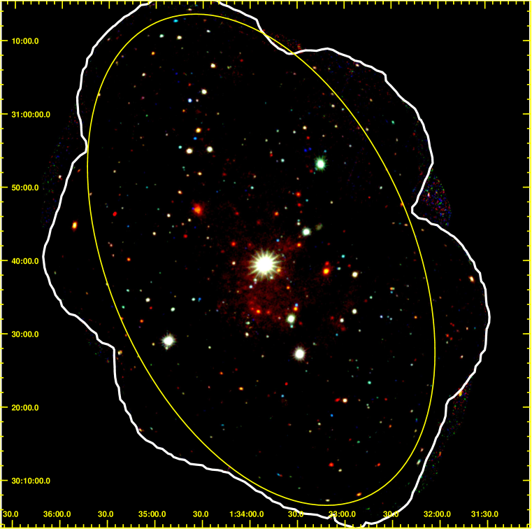
Figure 1.— Our color composite image of M33 from all of the observations listed in Table 1. Yellow ellipse marks the M33 D₂₅ region, and the white contour marks the area with at least 40 ks of exposure. Red is 0.2-0.5 keV. Green is 1-2 keV, and Blue is 2-4.5 keV.

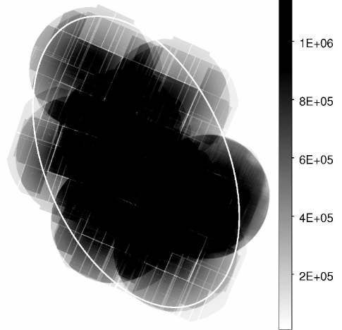
Figure 2.— Our total exposure map (0.2-4.5 keV) from the survey data listed in Table 1. This map was produced by emosaic_prep and includes the effects of vignetting. The ellipse marks the M33 D₂₅ region. The grayscale has units of summed PN, MOS1, and MOS2 seconds.

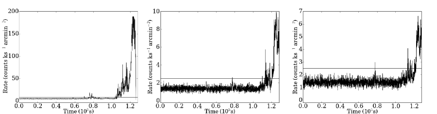
Figure 3.— Light curves for Field 6, showing typical flaring. Left is PN; middle is MOS1; right is MOS2. Horizontal lines mark our cuts for determining GTIs.

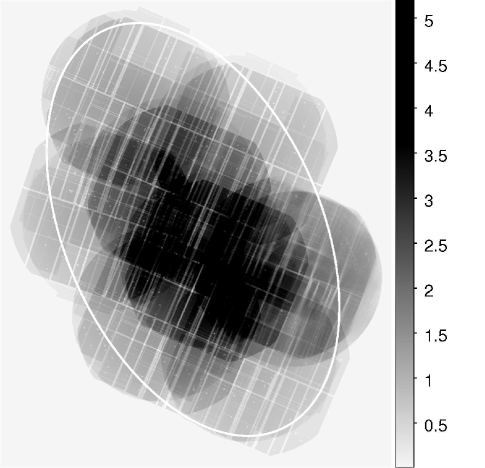
Figure 4.— Our total background map (0.2-4.5 keV) from the survey data listed in Table 1. The ellipse marks the M33 D₂₅ region. Grayscale has units of counts pixel^-1 (2.25^′′ pixel^-1).

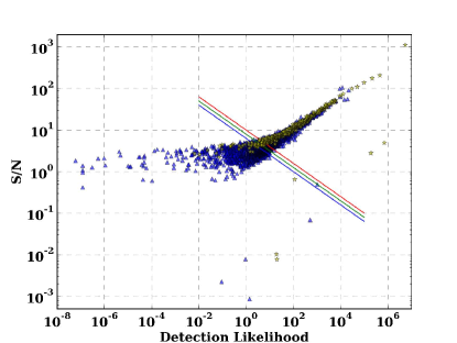
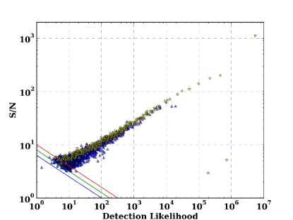
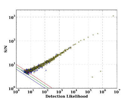
Figure 5.— Top: Signal-to-noise vs. DL for all of the source candidates from eboxdetect prior to making our quality cut. Blue triangles mark the measurements when data from all instruments from 0.2-4.5 keV are included. Stars mark sources matched with the catalog of T11, and diagonal lines mark possible quality cuts. The green line marks the cut we used for the final catalog. Middle: Same as top for our final catalog. Bottom: Same as top, but for our final catalog and showing only sources inside the T11 footprint.

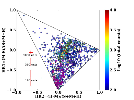
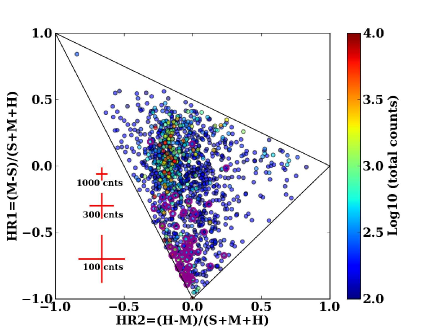
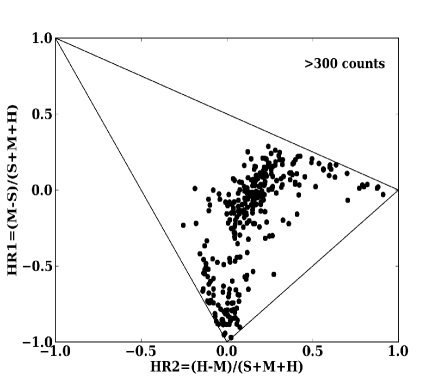
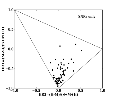
Figure 6.— Top left: Hardness ratios from fluxes in the 0.2-1.0, 1.0-2.0, and 2.0-4.5 keV bands of all unflagged, s-flagged, t-flagged, or matched to T11 sources with $>$50 source counts in Table 3. These fluxes use the ECFs in Table 2, which assume a power-law spectrum with index 1.7 and absorption 6$\times$10²⁰ cm^-2. The 0.2-1.0 keV fluxes are the sum of the 0.2-0.5 keV and 0.5-1.0 keV fluxes in Table 3. Fluxes are used for the HRs in this plot to make our catalog easier to compare with those measured with other X-ray observatories. H = 2.0-4.5 keV flux; M = 1.0-2.0 keV flux; S=0.2-1.0 keV flux. Upper limits were applied in bands with 0 counts to calculate ratios, so that no sources fall outside of the area allowed by positive flux measurements. Blue to red colors show the number of counts in the measurement. Known SNRs are highlighted with purple circles. Approximate uncertainties for a range of total counts are shown with the red crosses. Top right: Same as top-left, but ratios were calculated from count rates. Bottom left: Same as top-left, but without color-coding and showing only sources with $>$300 source counts in our catalog are shown. The sequence from the soft thermal sources to the hard, absorbed power-law sources is much clearer. Bottom right: Same as top-left, but without color-coding and showing only known SNRs, which have a markedly softer distribution than the full source population.

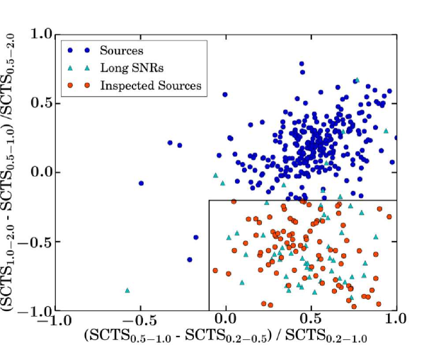
Figure 7.— Hardness ratio from source counts (SCTS) in the 0.2-0.5, 0.5-1.0, and 1.0-2.0 keV bands of all unflagged, s-flagged, t-flagged, or matched to T11 sources in our catalog with hardness ratio uncertainties $\leq$0.2 based on the number of counts in these bands. We use these ratios with the counts to make the same comparisons as Pietsch et al. (2004) for separating SNRs and foreground stars from sources with harder spectra. The black box indicates the region where most Long et al. (2010) SNRs (triangles) lie. The other sources in this box, indicated by the 89 orange dots, were not in the Long et al. (2010) catalog. These 89 were all investigated in optical images, and classified as SNRs if they coincided with gas emission or foreground stars if they coincided with a bright star. Sixty-two of the 89 remain unclassified.

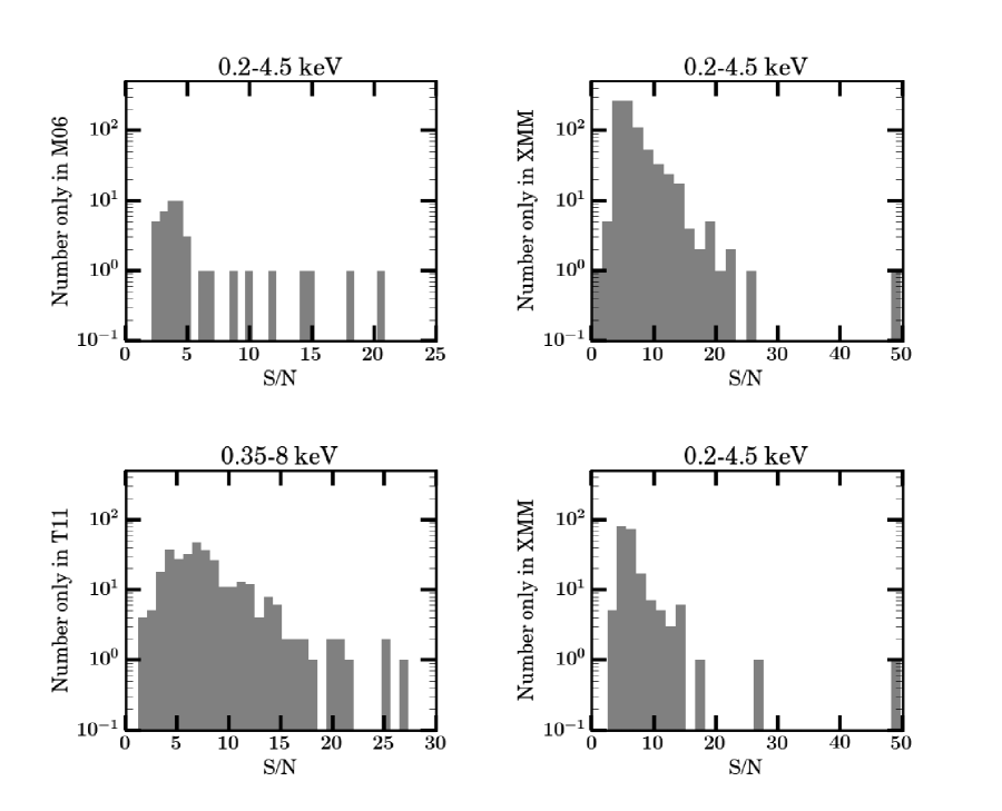
Figure 8.— Unmatched sources as a function of signal-to-noise of the detection in the 3 matched catalogs (M06, T11, this work). Upper-left S/N of sources in M06 unmatched to our catalog. Upper-right S/N of sources in our catalog unmatched to M06. Lower-left S/N of sources in T11 unmatched to our catalog. Lower-right S/N of sources in our catalog within the T11 footprint, but unmatched to any T11 source.

     

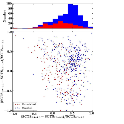
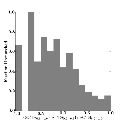
Figure 9.— Left Bottom: Hardness ratios optimized for separating soft sources using source counts (SCTS) in the 0.2-0.5, 0.5-1.0, and 1.0-2.0 keV energy bands of all matched sources inside of the T11 footprint (blue circles) and unmatched sources with 3$<$S/N$<$8 from our catalog inside the T11 footprint (red circles). SCTS are used for the hardness ratios in this case to directly compare the relative hardness of the newly-detected sources with the rest of the catalog. There are two sources with zero counts in the 0.5-1.0 keV band, one in the “unmatched” category and one in the “matched” category. The median uncertainty on the X-axis is 0.16 for the matched sources and 0.25 for the unmatched sources. The median uncertainty on Y-axis is 0.11 for the matched sources and 0.23 for the unmatched sources. Left Top: Sandpile histogram of all sources shown in left bottom so that the contribution of each to the total in each bin can be compared. The blue area shows the contribution of all matched sources; the red shows the contribution of unmatched sources. The unmatched sources have a softer distribution than the overall distribution. Right: Fraction of unmatched sources as a function of hardness ratio, showing that a high fraction of soft sources are not matched to a T11 source.

Figure 10.— Power spectra and lightcurves for two examples of observations of Source 763. Top Left: Power spectrum from observation 0650510201, showing a clear detection of variability at low frequencies in the power spectrum. Top Right: The variability suspected by inspecting the power spectrum is confirmed with a variable lightcurve. Bottom Left: Same as top left, but for observation 0650510601, which is a more borderline case. Here variability is seen at much lower significance at low frequencies in the power spectrum. Bottom Right: Same as top right, but for observation 0650510601. Again the detection is weaker, but variability is confirmed in the lightcurve.

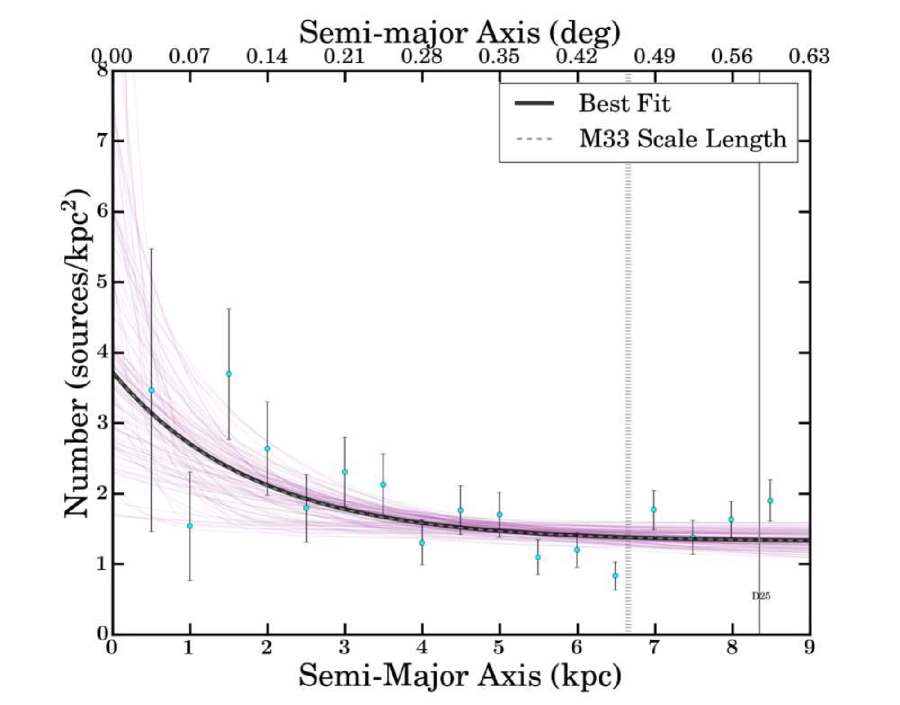
Figure 11.— X-ray source surface density for all sources with L${}_{0.2-4.5}{>}3.6{\times}10^{35}$ erg s^-1 and flags described in Section 4.2. Thick black line shows an exponential with scale length 1.8 kpc (best fit) and constant background of 1.3 kpc^-2. For comparison, the optical scale length (1.8 kpc) is plotted with a gray dashed line, which lies on top of the black line. A random draw of 100 trials from the MCMC runs used for uncertainty determination is shown with the thin pink lines. A constant surface density, which we take to be the background surface density, is reached by 6.7 kpc (marked with the vertical dotted line) and is relatively well-constrained, while the scale length is less certain due to the large error bars in the inner disk. D₂₅ is marked with the vertical gray line.

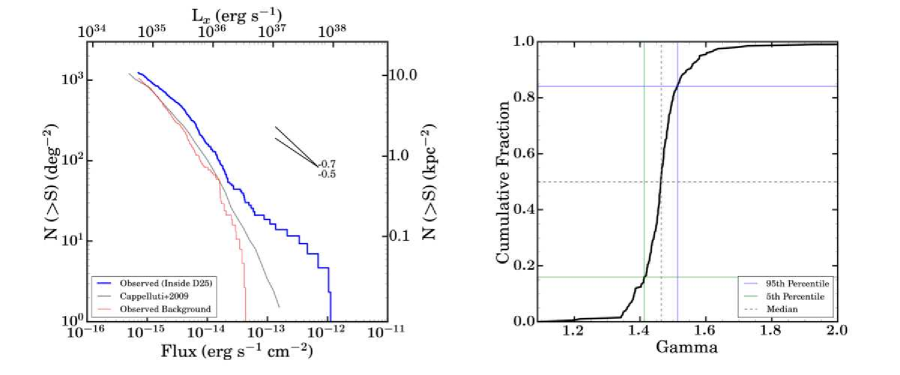
Figure 12.— Left: Cumulative luminosity function of all sources with fluxes $>$6$\times$10^-16 erg cm^-2 s^-1 inside of 6.7 kpc (deprojected) is shown in blue. Cumulative power-law indices of 0.5 and 0.7 (equivalent to 1.5 and 1.7 differential indices) are shown for comparison. The cosmic mean background shown in gray is taken from Cappelluti et al. (2009). The observed background, shown in red, is measured from our data outside of 6.7 kpc. Right: Cumulative distribution of the best fit power law index of the M33 component of the XLF from fits to our Monte Carlo draws from the catalog fluxes. The resulting 90% uncertainties to the best fit are 1.50${}^{+0.08}_{-0.14}$.

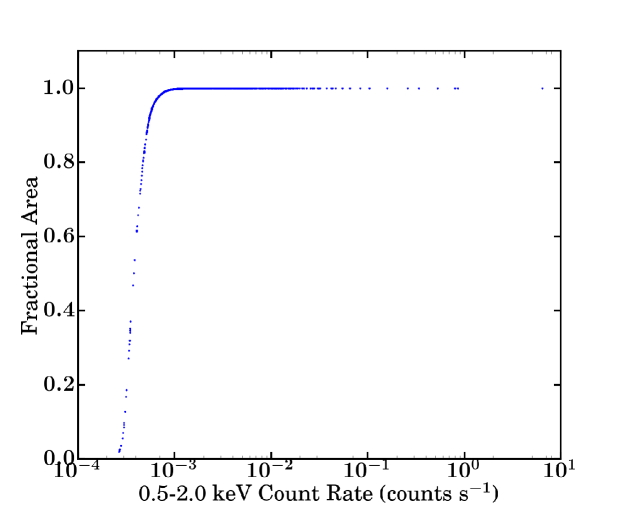
Figure 13.— Our fractional coverage of the area inside 6.7 kpc (deprojected) as a function of 0.5-2.0 keV count rate, as calculated from our combined sensitivity map. The entire area is covered down to a count rate of $\sim$8$\times$10^-4 counts s^-1.

References

- Arnaud (1996) Arnaud, K. A. 1996, in Astronomical Society of the Pacific Conference Series, Vol. 101, Astronomical Data Analysis Software and Systems V, ed. G. H. Jacoby & J. Barnes, 17
- Binder et al. (2012) Binder, B., et al. 2012, ApJ, 758, 15
- Broos et al. (2007) Broos, P. S., Feigelson, E. D., Townsley, L. K., Getman, K. V., Wang, J., Garmire, G. P., Jiang, Z., & Tsuboi, Y. 2007, ApJS, 169, 353
- Broos et al. (2010) Broos, P. S., Townsley, L. K., Feigelson, E. D., Getman, K. V., Bauer, F. E., & Garmire, G. P. 2010, ApJ, 714, 1582
- Broos et al. (2011) Broos, P. S., et al. 2011, ApJS, 194, 2
- Cappelluti et al. (2009) Cappelluti, N., et al. 2009, A&A, 497, 635
- Cash (1979) Cash, W. 1979, ApJ, 228, 939
- de Vaucouleurs et al. (1991) de Vaucouleurs, G., de Vaucouleurs, A., Corwin, H. G., Jr., Buta, R. J., Paturel, G., & Fouqué, P. 1991, Third Reference Catalogue of Bright Galaxies. Volume I: Explanations and references. Volume II: Data for galaxies between 0h and 12h. Volume III: Data for galaxies between 12h and 24h. (Springer, New York, NY (USA))
- Dodorico et al. (1980) Dodorico, S., Dopita, M. A., & Benvenuti, P. 1980, A&AS, 40, 67
- Foreman-Mackey et al. (2013) Foreman-Mackey, D., Hogg, D. W., Lang, D., & Goodman, J. 2013, PASP, 125, 306
- Freedman et al. (2001) Freedman, W. L., et al. 2001, The Astrophysical Journal, 553, 47
- Gordon et al. (1998) Gordon, S. M., Kirshner, R. P., Long, K. S., Blair, W. P., Duric, N., & Smith, R. C. 1998, ApJS, 117, 89
- Grimm et al. (2003) Grimm, H.-J., Gilfanov, M., & Sunyaev, R. 2003, MNRAS, 339, 793
- Grimm et al. (2005) Grimm, H.-J., McDowell, J., Zezas, A., Kim, D.-W., & Fabbiano, G. 2005, ApJS, 161, 271
- Grimm et al. (2007) Grimm, H.-J., McDowell, J., Zezas, A., Kim, D.-W., & Fabbiano, G. 2007, ApJS, 173, 70
- Haberl & Pietsch (2001) Haberl, F., & Pietsch, W. 2001, A&A, 373, 438
- Haberl et al. (2012) Haberl, F., et al. 2012, A&A, 545, A128
- Hartman et al. (2006) Hartman, J. D., Bersier, D., Stanek, K. Z., Beaulieu, J.-P., Kaluzny, J., Marquette, J.-B., Stetson, P. B., & Schwarzenberg-Czerny, A. 2006, MNRAS, 371, 1405
- Hatzidimitriou et al. (2006) Hatzidimitriou, D., Pietsch, W., Misanovic, Z., Reig, P., & Haberl, F. 2006, A&A, 451, 835
- Kuntz & Snowden (2008) Kuntz, K. D., & Snowden, S. L. 2008, A&A, 478, 575
- Long et al. (1990) Long, K. S., Blair, W. P., Kirshner, R. P., & Winkler, P. F. 1990, ApJS, 72, 61
- Long et al. (2010) Long, K. S., et al. 2010, ApJS, 187, 495
- Long et al. (1996) Long, K. S., Charles, P. A., Blair, W. P., & Gordon, S. M. 1996, ApJ, 466, 750
- Long et al. (1981) Long, K. S., Dodorico, S., Charles, P. A., & Dopita, M. A. 1981, ApJ, 246, L61
- Markert & Rallis (1983) Markert, T. H., & Rallis, A. D. 1983, ApJ, 275, 571
- Massey et al. (2006) Massey, P., Olsen, K. A. G., Hodge, P. W., Strong, S. B., Jacoby, G. H., Schlingman, W., & Smith, R. C. 2006, AJ, 131, 2478
- Mineo et al. (2012) Mineo, S., Gilfanov, M., & Sunyaev, R. 2012, MNRAS, 419, 2095
- Misanovic et al. (2006) Misanovic, Z., Pietsch, W., Haberl, F., Ehle, M., Hatzidimitriou, D., & Trinchieri, G. 2006, A&A, 448, 1247
- Pietsch et al. (2009) Pietsch, W., et al. 2009, ApJ, 694, 449
- Pietsch et al. (2003) Pietsch, W., Ehle, M., Haberl, F., Misanovic, Z., & Trinchieri, G. 2003, Astronomische Nachrichten, 324, 85
- Pietsch et al. (2006) Pietsch, W., Haberl, F., Sasaki, M., Gaetz, T. J., Plucinsky, P. P., Ghavamian, P., Long, K. S., & Pannuti, T. G. 2006, ApJ, 646, 420
- Pietsch et al. (2004) Pietsch, W., Misanovic, Z., Haberl, F., Hatzidimitriou, D., Ehle, M., & Trinchieri, G. 2004, A&A, 426, 11
- Plucinsky et al. (2008) Plucinsky, P. P., et al. 2008, ApJS, 174, 366
- Schulman & Bregman (1995) Schulman, E., & Bregman, J. N. 1995, ApJ, 441, 568
- Stark et al. (1992) Stark, A. A., Gammie, C. F., Wilson, R. W., Bally, J., Linke, R. A., Heiles, C., & Hurwitz, M. 1992, ApJS, 79, 77
- Stiele et al. (2011) Stiele, H., Pietsch, W., Haberl, F., Hatzidimitriou, D., Barnard, R., Williams, B. F., Kong, A. K. H., & Kolb, U. 2011, A&A, 534, A55
- Strüder et al. (2001) Strüder, L., et al. 2001, A&A, 365, L18
- Trudolyubov (2013) Trudolyubov, S. P. 2013, MNRAS, 435, 3326
- Tüllmann et al. (2011) Tüllmann, R., et al. 2011, ApJS, 193, 31
- Tüllmann et al. (2009) Tüllmann, R., et al. 2009, ApJ, 707, 1361
- Turner et al. (2001) Turner, M. J. L., et al. 2001, A&A, 365, L27
- Williams et al. (2009) Williams, B. F., Dalcanton, J. J., Dolphin, A. E., Holtzman, J., & Sarajedini, A. 2009, ApJ, 695, L15
- Williams et al. (2008) Williams, B. F., et al. 2008, ApJ, 680, 1120
- XMM-Newton Survey Science Centre (2013) XMM-Newton Survey Science Centre, C. 2013, VizieR Online Data Catalog, 9044, 0