Fourth-order split monopole perturbation solutions
to the Blandford-Znajek mechanism

Abstract

The Blandford-Znajek (BZ) mechanism describes a physical process for the energy extraction from a spinning black hole (BH), which is believed to power a great variety of astrophysical sources, such as active galactic nuclei (AGNs) and Gamma ray bursts (GRBs). The only known analytic solution to the BZ mechanism is a split monopole perturbation solution up to $O(a^{2})$, where $a$ is the spin parameter of a Kerr black hole. In this paper, we extend the monopole solution to higher order $\sim O(a^{4})$. We carefully investigate the structure of the BH magnetosphere, including the angular velocity of magnetic field lines $\Omega$, the toroidal magnetic field $B^{\phi}$ as well as the poloidal electric current $I$. In addition, the relevant energy extraction rate $\dot{E}$ and the stability of this high-order monopole perturbation solution are also examined.

I Introduction

Within the framework of force-free electrodynamics, Blandford & Znajek (1977) investigated a steady-state axisymmetric magnetsphere surrounding a spinning black hole and put forward that the rotation energy of a Kerr black hole could be extracted in the form of Poynting flux via magnetic fields penetrating the central black hole (Blandford and Znajek (1977); Lee et al. (2000)). General relativistic magnetodynamics (GRMD) simulations of split monopole magnetic fields (Komissarov (2001, 2004)) show that the analytic monopole perturbation solution makes good matches with the numerical simulations, especially for slowly rotating black holes. General relativistic magnetohydrodynamics (GRMHD) simulations (McKinney and Gammie (2004); McKinney (2005)) indicate that, in the polar region, the monopole perturbation solution gives a good description of the magnetic field configuration as well as the angular distribution of energy flow, even when black holes rotate mildly rapidly. However, the monople solution Blandford and Znajek (1977) is accurate only up to $O(a^{2})$, where $a$ is the black hole spin parameter. For even more rapidly rotating black holes, higher order perturbation solutions are of greater astrophysical interests. Tanabe and Nagataki (2008) extended the monopole perturbation solution to the order of $O(a^{4})$. Their solution gave a better approximation to the numerical simulation. Unfortunately, they mentioned that their results are not fully self-consistent, since their perturbation method breaks down at large distance from the central black hole. Hence, it is necessary to find self-consistent higher order perturbation solutions to the BZ mechanism.

To get self-consistent solutions, we need to solve a nonlinear second-order partial differential equation, which requires two boundary conditions. It should be noted that boundary conditions to be imposed are still not well understood (Uzdensky (2004, 2005); Tanabe and Nagataki (2008); Beskin (2004); Nathanail and Contopoulos (2014)). Blandford and Znajek (1977) imposed the Znajek regularity condition (Znajek (1977)) on the horizon as the first boundary condition. The second one requires that the perturbation solution should match the asymptotic solution in the flat spacetime at infinity (Michel (1973)). Unfortunately, the second boundary condition is usually unavailable when investigating higher order perturbation solutions. Recently, Pan and Yu (2014) proposed that the physical constraint, i.e., solutions should be convergent from the horizon to infinity, could be exploited as the second boundary condition. With the Znajek horizon regularity condition and this new convergence constraint, perturbation solutions could be uniquely determined. Following the approach of Pan and Yu (2014), we extend the monopole perturbation solution to the order of $O(a^{4})$. Note that the perturbation method we adopt is different from Tanabe and Nagataki (2008). Our method works well at any distance from the central black hole.

Some earlier analytic works (Li (2000); Lyutikov (2006); Giannios and Spruit (2006)) concerned the stability of jets launched by the BZ mechanism because of the screw instability of the magnetic field. However, such instability was not found in recent simulations (e.g. McKinney and Blandford (2009); Tchekhovskoy et al. (2010); McKinney et al. (2013)). The possible reason for the discrepancy is that the Krustkal-Shafranov (KS) criteria is used in these works, without taking account of the stabilizing effect induced by the magnetic field rotation (Tomimatsu et al. (2001); McKinney and Blandford (2009); O’Neill et al. (2012)). With the high-order perturbation solution obtained in this paper, we also briefly study the stability of the split monopole perturbation solution of the order of $O(a^{4})$, taking the magnetic field rotation into consideration.

The paper is organized as follows: basic equations governing stationary axisymmetric force-free fields around Kerr black holes are described in section II. We discuss the perturbation solutions of second-order and fourth-order obtained by our newly proposed method in section III. Summary and discussion are given in section IV.

II Stationary Axisymmetric Force-Free Fields around Kerr Black Holes

In this section, we briefly recap basic equations governing stationary axisymmetric force-free fields around Kerr black holes (see Pan and Yu (2014) and references therein for more details). We adopt the Kerr-Schild coordinate (e.g., McKinney and Gammie (2004)) with the line element

$$ds^{2}=-\left(1-\frac{2r}{\Sigma}\right)dt^{2}+\left(\frac{4r}{\Sigma}\right)drdt+\left(1+\frac{2r}{\Sigma}\right)dr^{2}+\Sigma d\theta^{2}-\frac{4ar\sin^{2}\theta}{\Sigma}d\phi dt$$

$$-2a\left(1+\frac{2r}{\Sigma}\right)\sin^{2}\theta d\phi dr+\sin^{2}\theta\left[\Delta+\frac{2r(r^{2}+a^{2})}{\Sigma}\right]d\phi^{2}\ ,$$ (1)

where $\Sigma=r^{2}+a^{2}\cos^{2}\theta$, $\Delta=r^{2}-2r+a^{2}$, and $\sqrt{-g}=\Sigma\sin\theta$ .

The energy momentum tensor for the force-free field is dominated by the electro-magnetic field, which can be written as $T^{\mu\nu}=T^{\mu\nu}_{\rm matter}+T^{\mu\nu}_{\rm EM}\approx T^{\mu\nu}_{\rm EM}=F^{\mu\tau}F^{\nu}_{\phantom{nu}\tau}-\frac{1}{4}\delta^{\mu\nu}F^{\alpha\beta}F_{\alpha\beta}$, where the antisymmetric Faraday tensor is defined as $F_{\mu\nu}=\partial_{\mu}A_{\nu}-\partial_{\nu}A_{\mu}$ and $A$ is the $4-$potential of electromagnetic field. We define the angular velocity of the magnetic field $\Omega(r,\theta)$ as follows,

$$-\Omega\equiv\frac{dA_{t}}{dA_{\phi}}=\frac{A_{t,\theta}}{A_{\phi,\theta}}=\frac{A_{t,r}}{A_{\phi,r}}\ .$$ (2)

It is evident that $F_{t\phi}=0$ for the axisymmetric and steady state force-free field. The non-zero parts of the Faraday tensor $F_{\mu\nu}$ are listed below:

$$F_{r\phi}=-F_{\phi r}=A_{\phi,r}\ ,F_{\theta\phi}=-F_{\phi\theta}=A_{\phi,\theta}\ ,$$ (3)

$$F_{tr}=-F_{rt}=\Omega A_{\phi,r}\ ,F_{t\theta}=-F_{\theta t}=\Omega A_{\phi,\theta}\ ,$$ (4)

$$F_{r\theta}=-F_{\theta r}=\sqrt{-g}B^{\phi}\ .$$ (5)

Note that the force-free field is specified by three quantities, i.e., $\Omega(r,\theta)$, $A_{\phi}(r,\theta)$, and $B^{\phi}(r,\theta)$. Once they are specified, the force-free field is uniquely determined.

Note that $T^{\theta}_{\phantom{\theta}t}=-\Omega T^{\theta}_{\phantom{\theta}\phi}$ and $T^{r}_{\phantom{r}t}=-\Omega T^{r}_{\phantom{r}\phi}$. The energy and angular momentum conservation equations $T^{\mu}_{\phantom{\mu}t;\mu}=0$ and $T^{\mu}_{\phantom{\mu}\phi;\mu}=0$ can be cast as $\Omega_{,r}A_{\phi,\theta}=\Omega_{,\theta}A_{\phi,r}$ and $(\sqrt{-g}F^{\theta r})_{,r}A_{\phi,\theta}=(\sqrt{-g}F^{\theta r})_{,\theta}A_{\phi,r}$, respectively. These two equations indicate that $\Omega$ and $\sqrt{-g}F^{\theta r}$ are functions of $A_{\phi}$, viz,

$$\Omega\equiv\Omega(A_{\phi})\ ,\ \sqrt{-g}F^{\theta r}\equiv I(A_{\phi})\ ,$$ (6)

where the angular velocity of magnetic field $\Omega$ and the poloidal electric current $I$ are to be specified. Substituting Equations (3), (4), (5) and (6) into the equation $F^{\theta r}=g^{\theta\mu}g^{r\nu}F_{\mu\nu}$, we can readily arrive at

$$B^{\phi}=-\frac{I\Sigma+(2\Omega r-a)\sin\theta A_{\phi,\theta}}{\Delta\Sigma\sin^{2}\theta}\ .$$ (7)

This is an important relation that connects the toroidal magnetic field $B^{\phi}$ with the functions $A_{\phi}(r,\theta)$, $\Omega(A_{\phi})$ and $I(A_{\phi})$.

The remaining momentum conservation equations in the $r$ and $\theta$ direction $T^{\mu}_{\phantom{\mu}r;\mu}=0$ and $T^{\mu}_{\phantom{\mu}\theta;\mu}=0$ are actually equivalent and read

$$-\Omega\left[(\sqrt{-g}F^{tr})_{,r}+(\sqrt{-g}F^{t\theta})_{,\theta}\right]+F_{r\theta}I^{\prime}(A_{\phi})+\left[(\sqrt{-g}F^{\phi r})_{,r}+(\sqrt{-g}F^{\phi\theta})_{,\theta}\right]=0\ ,$$ (8)

where the prime denotes derivative with respect to $A_{\phi}$. The three functions $A_{\phi}(r,\theta)$, $\Omega(A_{\phi})$, and $I(A_{\phi})$ are related by the above nonlinear equation (8), which is also widely known as the Grad-Shafranov (GS) equation (Uzdensky (2005); Contopoulos et al. (2013)).

III Fourth-order Perturbation Solutions

Since the Farady tensor depends on the first order derivative of $A_{\phi}$, it is clear that the GS equation (8) is actually a second-order partial differential equation for $A_{\phi}$. The solution can be attained when complemented with two boundary conditions, i.e., the Znajek horizon regularity condition (Znajek (1977)) and the convergence constraint (Blandford and Znajek (1977); Pan and Yu (2014)). The zeroth-order monopole solution can be readily obtained when the black hole is non-rotating, i.e., $a=0$. When the spin parameter $a\neq 0$, we expand the GS equation in terms of $a$. To get the second-order perturbation solutions, we ignore all terms in the GS equation that are higher than the order of $O(a^{2})$. Based on the second-order solutions, the fourth-order perturbation solution can be achieved in a similar way.

The zeroth-order monopole solution around non-rotating black hole can be explicitly written as (Blandford and Znajek (1977)),

$$\Omega_{0}=0,\qquad B^{\phi}_{0}=0,\qquad A_{\phi}=A_{0}=-\cos\theta.$$ (9)

Since $\Omega$ and $\sqrt{-g}F^{\theta r}$ are functions of $A_{\phi}$, we can expand them, accurate to the order of $O(a^{4})$, as

$$\Omega = \Omega(A_{\phi})=a\omega_{1}(A_{\phi})+a^{3}\omega_{3}(A_{\phi})=a\omega_{1}(A_{0}+a^{2}A_{2})+a^{3}\omega_{3}(A_{0}+a^{2}A_{2}),$$

$$\sqrt{-g}F^{\theta r} = I(A_{\phi})=ai_{1}(A_{\phi})+a^{3}i_{3}(A_{\phi})=ai_{1}(A_{0}+a^{2}A_{2})+a^{3}i_{3}(A_{0}+a^{2}A_{2}),$$ (10)

where $\Omega$, $\omega_{1}$, $\omega_{3}$, $I$, $i_{1}$, $i_{3}$ are unknown functions of $A_{\phi}$ to be specified self-consistently. The entire fourth-order perturbation solutions can be expressed in a more compact form as,

$$A_{\phi} = A_{0}+a^{2}A_{2}+a^{4}A_{4}+O(a^{6})\ ,$$

$$\Omega = a\Omega_{1}+a^{3}\Omega_{3}+O(a^{5})\ ,$$

$$\sqrt{-g}F^{\theta r} = aI_{1}+a^{3}I_{3}+O(a^{5})\ ,$$

$$B^{\phi} = aB_{1}+a^{3}B_{3}+O(a^{5})\ .$$ (11)

It should be noted that $\Omega_{n}$ and $\omega_{n}$, $I_{n}$ and $i_{n}$ ($n=1,3$) are related by

$$\Omega_{1} = \omega_{1}(A_{0})\ ,\qquad\Omega_{3}=\omega_{1}^{\prime}(A_{0})A_{2}+\omega_{3}(A_{0})\ ,$$

$$I_{1} = i_{1}(A_{0})\ ,\qquad\,I_{3}=i_{1}^{\prime}(A_{0})A_{2}+i_{3}(A_{0})\ ,$$ (12)

where the prime designates the derivative with respect to $A_{0}$.

III.1 Second-order Perturbation Solutions

We can get the second-order perturbation solutions by expanding the GS equation (8) to the order of $O(a^{2})$. It is interesting that the original BZ monopole perturbation solution could be naturally achieved with our convergence constraint. Expanding Eq.(7) to the order of $O(a^{2})$, we have that

$$r^{2}I_{1}=\sin\theta A_{0,\theta}(1-2r\Omega_{1})-\sin^{2}\theta B_{1}(r^{2}-2r)r^{2}.$$ (13)

According to the Znajek horizon condition (Znajek (1977)), the toroidal field $B_{1}$ should be well-behaved on the horizon $(r=2)$, then $r=2$ must be a root to equation $r^{2}I_{1}=\sin^{2}\theta(1-2r\Omega_{1})$. So we have

$$i_{1} = I_{1}=\sin^{2}\theta\left(\frac{1}{4}-\Omega_{1}\right),$$

$$B_{1} = -\frac{1}{r^{2}}\left(\frac{1}{4}-\Omega_{1}+\frac{1}{2r}\right).$$ (14)

The GS equation (8), accurate to the order of $O(a^{2})$, can then be cast as

$$\mathcal{L}A_{2}=S(r,\theta)\ ,$$ (15)

where the operator

$$\mathcal{L}\equiv\frac{1}{\sin\theta}\frac{\partial}{\partial r}\left(1-\frac{2}{r}\right)\frac{\partial}{\partial r}+\frac{1}{r^{2}}\frac{\partial}{\partial\theta}\frac{1}{\sin\theta}\frac{\partial}{\partial\theta}\ ,$$ (16)

and the source

$$S(r,\theta) = 4\sin\theta\cos\theta\left(\Omega_{1}-\frac{1}{8}\right)\left(\frac{1}{4}+\frac{1}{2r}+\frac{1}{r^{2}}\right)-2\sin\theta\cos\theta\frac{1}{r^{2}}\left(\frac{1}{2r}+\frac{1}{r^{2}}\right)$$ (17)

$$+\sin^{2}\theta\Omega_{1,\theta}\left(\frac{1}{4}+\frac{1}{2r}+\frac{1}{r^{2}}\right).$$

According to Blandford and Znajek (1977), the condition for the existence of solution is that the following integral,

$$\int_{2}^{\infty}dr\int_{0}^{\pi}d\theta\frac{|S(r,\theta)|}{r}\ ,$$ (18)

should be convergent. The convergence condition requires all the terms in $S(r,\theta)$ of the order of $O(1)$ should vanish, i.e.,

$$0=4\sin\theta\cos\theta\left(\Omega_{1}-\frac{1}{8}\right)+\sin^{2}\theta\Omega_{1,\theta}\ .$$ (19)

Consequently, we have

$$\Omega_{1} = \omega_{1}=\frac{1}{8}\ ,$$

$$I_{1} = i_{1}=\frac{1}{8}\sin^{2}\theta\ ,$$

$$B_{1} = -\frac{1}{r^{2}}\left(\frac{1}{8}+\frac{1}{2r}\right)\ .$$ (20)

It is interesting to note that all physical quantities of the order $O(a)$ are already obtained before we actually solve the complicated GS equation. The second-order part of $A_{\phi}$, i.e., $A_{2}$, can be obtained by the following equation,

$$\mathcal{L}A_{2}=-2\sin\theta\cos\theta\frac{1}{r^{2}}\left(\frac{1}{2r}+\frac{1}{r^{2}}\right)\ .$$ (21)

It is straightforward while tedious to check that this equation has the following variable separable solution(Blandford and Znajek (1977))

$$A_{2}=R(r)\sin^{2}\theta\cos\theta,$$ (22)

where

$$R(r)=\frac{1+3r-6r^{2}}{12}\ln\left(\frac{r}{2}\right)+\frac{11}{72}+\frac{1}{3r}+\frac{r}{2}-\frac{r^{2}}{2}$$

$$\qquad\qquad\qquad\qquad+\left[\mathrm{Li}_{2}\left(\frac{2}{r}\right)-\ln\left(1-\frac{2}{r}\right)\ln\left(\frac{r}{2}\right)\right]\frac{r^{2}(2r-3)}{8}\ ,$$ (23)

and

$$\mathrm{Li}_{2}(x)=-\int_{0}^{1}dt\frac{\ln(1-tx)}{t}\ .$$ (24)

The value of the function $R(r)$ at the horizon, $r=2$, is of particular importance. Explicitly, it is

$$R_{r=2}=R({r=2})=\frac{6\pi^{2}-49}{72}\ .$$ (25)

III.2 Fourth-order Perturbation Solutions

Once the second-order perturbation solutions are known, the fourth-order perturbation solutions could be obtained by further expanding the GS equation to the order of $O(a^{4})$ . Accurate to $O(a^{4})$, Eq.(7) is

$$r^{2}I_{3}+\cos^{2}\theta I_{1}=\sin\theta\left[A_{2,\theta}(1-2r\Omega_{1})-A_{0,\theta}2r\Omega_{3}\right]$$

$$\qquad\qquad\qquad-\sin^{2}\theta\left[B_{3}(r^{2}-2r)r^{2}+B_{1}(r^{2}-2r)\cos^{2}\theta+B_{1}r^{2}\right]\ .$$ (26)

The toroidal field $B_{3}$ should be well behaved on the horizon. Subsequently, we can get

$$i_{3}+\sin^{2}\theta\omega_{3}=\left(-\frac{R_{r=2}}{8}+\frac{1}{32}\right)\sin^{4}\theta+\frac{1}{16}\sin^{2}\theta,$$ (27)

and the toroidal field $B_{3}$ is

$$\sin^{2}\theta B_{3}=\frac{1}{r^{2}-2r}\bigg{[} -\frac{2\sin^{2}\theta}{r}\omega_{3}+\left(\frac{1}{r^{2}}-\frac{1}{4r}\right)\sin\theta\left(A_{2,\theta}-\frac{\sin\theta\cos^{2}\theta}{r^{2}}\right)$$ (28)

$$+\frac{\sin^{2}\theta}{r^{2}}\left(\frac{1}{8}+\frac{1}{2r}\right)-\left(\frac{\cos\theta}{4}A_{2}+i_{3}\right)\bigg{]},$$

where we have made use of Eq.(III) and (III.1). The GS equation (8) of the order of $O(a^{4})$ is of the following form,

$$\mathcal{L}A_{4} = \omega_{1}\left[\sin\theta\left(\frac{r^{2}}{8}-\frac{2}{r}\right)A_{2,r}\right]_{,r}-\omega_{3}\left[-\left(1+\frac{2}{r}\right)\frac{1}{8}\sin^{2}\theta+2r\sin^{2}\theta B_{1}\right]_{,\theta}$$

$$-\omega_{1}\left[-\sin\theta\left(1+\frac{2}{r}\right)\left(\frac{1}{8}A_{2,\theta}+\omega_{3}\sin\theta\right)+\frac{\sin^{2}\theta\cos^{2}\theta}{4r^{3}}+2r\sin^{2}\theta B_{3}\right]_{,\theta}$$

$$+r^{2}\sin\theta B_{1}\left[-\frac{1}{4}A_{2}+i_{3}^{\prime}(A_{0})\right]+\frac{1}{4}\cos\theta\sin\theta\left(\cos^{2}\theta B_{1}+r^{2}B_{3}\right)$$

$$-\left(\frac{\sin\theta}{4r}A_{2,r}+\frac{2\cos^{2}\theta}{r^{3}\sin\theta}A_{2,r}\right)_{,r}+\left(\sin^{2}\theta B_{3}+\frac{\cos^{2}\theta}{r^{4}\sin\theta}A_{2,\theta}-\frac{\cos^{4}\theta}{r^{6}}\right)_{,\theta}.$$

The convergence condition requires all source terms of the order $O(1)$ should vanish, i.e.,

$$0=\omega_{3}\left(\frac{1}{8}\sin^{2}\theta\right)_{,\theta}+\omega_{1}(\sin^{2}\theta\omega_{3})_{,\theta}+r^{2}\sin\theta B_{1}i_{3}^{\prime}(A_{0})+\frac{1}{4}\sin\theta\cos\theta r^{2}B_{3}\ .$$ (30)

The above equation could be further simplified as

$$\omega_{3}(\sin^{2}\theta)_{,\theta}+(\sin^{2}\theta\omega_{3})_{,\theta}=i_{3,\theta}+2\frac{\cos\theta}{\sin\theta}i_{3}=\frac{1}{\sin^{2}\theta}(\sin^{2}\theta i_{3})_{,\theta}\Leftrightarrow\sin^{2}\theta\omega_{3}=i_{3},$$ (31)

where we have used the result of Eq.(III.1) and (28). Together with Eq.(27), we have that

$$i_{3} = \frac{1}{2}\left(-\frac{R_{r=2}}{8}+\frac{1}{32}\right)\sin^{4}\theta+\frac{1}{32}\sin^{2}\theta,$$

$$\omega_{3} = \frac{1}{2}\left(-\frac{R_{r=2}}{8}+\frac{1}{32}\right)\sin^{2}\theta+\frac{1}{32}>\frac{1}{32}.$$ (32)

With the help of Eq.(III) and (III.1), we finally arrive at

$$\Omega=\Omega(A_{\phi}) = \frac{a}{8}+a^{3}\omega_{3},$$

$$\sqrt{-g}F^{\theta r}=I(A_{\phi}) = \frac{a}{8}\sin^{2}\theta+a^{3}\left(\frac{1}{4}R(r)\sin^{2}\theta\cos^{2}\theta+i_{3}\right).$$ (33)

IV Discussion and Summary

IV.1 Discussion

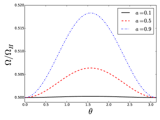
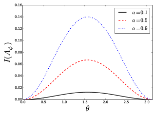
Figure 1: Angular distribution of the ratio $\Omega/\Omega_{H}$ and the electric current $I$ on horizon ($r=2$), where we keep the angular velocity of the BH accurate to fourth order, i.e., $\Omega_{H}=a/4+a^{3}/16$ .

The angular distribution of the fourth-order angular velocity $\Omega$ and poloidal eletric current $I$ on the horizon is shown in Fig.1. For comparison, the corresponding simulation results are also available (cf., Fig.1 and 2 of Komissarov (2001)). Both simulations and our analytic solution imply that $\Omega=\Omega_{H}/2$ is a rather good approximation for a wide range of black hole spins (at least for $a\lesssim 0.9$), where $\Omega_{H}=a/{2(1+\sqrt{1-a^{2}})}$ is the angular velocity of the central BH. The fourth-order poloidal electric current $I$ also shows better agreement with the simulation result than the second-order one, especially for large spins.

The energy extraction rate, which is defined as $\dot{E}=-2\pi\int_{0}^{\pi}\sqrt{-g}T^{r}_{\ t}d\theta=2\pi\int I(A_{\phi})\Omega(A_{\phi})dA_{\phi}$ (Blandford and Znajek (1977); Pan and Yu (2014); Beskin (2009)), could be written as

$$\dot{E} = 2\pi a^{2}\int i_{1}\omega_{1}dA_{0}+2\pi a^{4}\int i_{1}\omega_{3}+\omega_{1}i_{3}+(i_{1}\omega_{1}A_{2})^{\prime}dA_{0}$$ (34)

$$= 2\pi a^{2}\int i_{1}\omega_{1}dA_{0}+2\pi a^{4}\int\frac{1}{8}(i_{3}+\sin^{2}\theta\omega_{3})dA_{0}$$

$$= \frac{\pi}{24}a^{2}+\frac{(56-3\pi^{2})\pi}{1080}a^{4}$$

where the prime denotes derivative with respect to $A_{0}$. Note that the second term on the right hand side only depends on the combination, $i_{3}+\sin^{2}\theta\omega_{3}$, which can be specified by the Znajek horizon condition (i.e., Eq.(27)). In fact, this coincidence explains why Tanabe and Nagataki (2008) could obtain the correct energy extraction rate $\dot{E}$ without explicitly solving $\Omega$ and $I$.

The stability is another interesting issue. Some analytic works (Li (2000); Lyutikov (2006); Giannios and Spruit (2006)) implied that the screw instability may occur in the monopole perturbation solution due to the Kruskal-Shafranov criterion. But no instability was noticed in time-dependent GRMD (e.g. Komissarov (2001, 2004)) or GRMHD simulations (e.g. McKinney and Blandford (2009); McKinney et al. (2013)). To understand the discrepancy between analytic and numerical works, Narayan et al. (2009) (and Tomimatsu et al. (2001); McKinney and Blandford (2009)) pointed out that Kruskal-Shafranov criterion may not be appropriate for jet stability analysis, since it neglects the stabilizing effect of the rotation of magnetic field lines. According to the analysis of Tomimatsu et al. (2001), which takes the field rotation into account, the monopole perturbation solution is possibly unstable only when $\Omega<\Omega_{H}/2$. Our fourth order solution (i.e., Eq.(III.2)) means that

$$\Omega>\frac{1}{2}\Omega_{H}=\frac{a}{8}+\frac{a^{3}}{32}\ .$$ (35)

Obviously, the fourth-order monopole perturbation solution is stable and is consistent with numerical simulations.

IV.2 Summary

Two major difficulties are encountered in solving the GS equation (8): 1) it is a highly nonlinear second order partial differential equation; 2) two proper boundary conditions are necessary to uniquely specify the solution. The nonlinearity could be partially removed by the perturbation technique. To fix the boundary conditions problem, we impose the regularity condition on the horizon (Eq.(7)) and the convergence constraint (Eq.(18)). The latter one actually serves as the boundary condition at infinity. With these two boundary conditions, we re-establish the split monopole solution to the order of $O(a^{2})$ and get the new perturbation solution up to the order of $O(a^{4})$. By taking account of the stabilizing effect of field rotation, we prove that the fourth-order monopole perturbation solution is stable against the screw instability.