EUROPEAN ORGANIZATION FOR NUCLEAR RESEARCH (CERN)

​​​ CERN-PH-EP-2015-058 LHCb-PAPER-2014-068 June 18, 2015

Measurement of $C\!P$ asymmetries and polarisation fractions in ${{B}^{0}_{s}}\rightarrow{{K}^{*0}}{{\kern 4.14793pt\overline{\kern-4.14793ptK}{}}{}^{*0}}$ decays

The LHCb collaboration

An angular analysis of the decay ${{B}^{0}_{s}}\rightarrow{{K}^{*0}}{{\kern 1.99997pt\overline{\kern-1.99997ptK}{}}{}^{*0}}$ is performed using $pp$ collisions corresponding to an integrated luminosity of $1.0\,{\rm fb}^{-1}$ collected by the LHCb experiment at a centre-of-mass energy $\sqrt{s}=7\,{\rm TeV}$. A combined angular and mass analysis separates six helicity amplitudes and allows the measurement of the longitudinal polarisation fraction $f_{L}=0.201\pm 0.057{\ \rm(stat.)}\pm 0.040{\ \rm(syst.)}$ for the ${{B}^{0}_{s}}\rightarrow K^{*}(892)^{0}{\kern 1.99997pt\overline{\kern-1.99997ptK}{}}{}^{*}(892)^{0}$ decay. A large scalar contribution from the $K^{*}_{0}(1430)$ and $K^{*}_{0}(800)$ resonances is found, allowing the determination of additional $C\!P$ asymmetries. Triple product and direct $C\!P$ asymmetries are determined to be compatible with the Standard Model expectations. The branching fraction ${\cal B}({{B}^{0}_{s}}\rightarrow K^{*}(892)^{0}{\kern 1.99997pt\overline{\kern-1.99997ptK}{}}{}^{*}(892)^{0})$ is measured to be $(10.8\pm 2.1{\ \rm(stat.)}\pm 1.4{\ \rm(syst.)}\pm 0.6\ (f_{d}/f_{s}))\times 10^{-6}$.

Submitted to JHEP

© CERN on behalf of the LHCb collaboration, license CC-BY-4.0.

 

1 Introduction

The ${{B}^{0}_{s}}\rightarrow{{K}^{*0}}{{\kern 1.99997pt\overline{\kern-1.99997ptK}{}}{}^{*0}}$ decay is mediated by a $b\rightarrow sd\bar{d}$ flavour-changing neutral current (FCNC) transition, which in the Standard Model (SM) proceeds through loop diagrams at leading order. This decay has been discussed in the literature as a possible field for precision tests of the SM predictions, when it is considered in association with its U-spin symmetric channel ${{B}^{0}}\rightarrow{{K}^{*0}}{{\kern 1.99997pt\overline{\kern-1.99997ptK}{}}{}^{*0}}$ [1, 2, 3]. In the SM, the expected $C\!P$ violation in the former is very small, $\mathcal{O}(\lambda^{2})$, with approximate cancellation between the mixing and the decay CKM phases [4]. When a scalar meson background is allowed, in addition to the vector-vector meson states, six independent helicities contribute [4].

In this paper, a search for non-SM electroweak amplitudes is reported in the decay $B^{0}_{s}\rightarrow K^{+}\pi^{-}K^{-}\pi^{+}$, with $K\pi$ mass close to the $K^{*}(892)^{0}$ mass, through the measurement of all $C\!P$-violating observables accessible when the flavour of the bottom-strange meson is not identified. These observables include triple products (TPs) and other $C\!P$-odd quantities [5], many of which are, as yet, experimentally unconstrained. Triple products are $T$-odd observables having the generic structure $\bm{v_{1}}\cdot(\bm{v_{2}}\times\bm{v_{3}})$ where $\bm{v_{i}}$ is the spin or momentum of a final-state particle. In vector-vector final states of $B$ mesons they take the form $\bm{q}\cdot(\bm{\epsilon_{1}}\times\bm{\epsilon_{2}})$ where $\bm{q}$ is the momentum of one of the final vector mesons and $\bm{\epsilon_{1}}$ and $\bm{\epsilon_{2}}$ are their respective polarisations. Triple products are also meaningful when one of the final particles is a scalar meson.

Theoretical predictions based on perturbative QCD for the decay of $B$ mesons into scalar-vector final states $K^{*}_{0}(1430){\kern 1.99997pt\overline{\kern-1.99997ptK}{}}{}^{*}(892)^{0}$ have been recently investigated, yielding branching fractions comparable to those of vector-vector final states [6], which have been previously available [7]. The ${{B}^{0}_{s}}\rightarrow{{K}^{*0}}{{\kern 1.99997pt\overline{\kern-1.99997ptK}{}}{}^{*0}}$ decay was first observed with 35$\mbox{\,pb}^{-1}$ of LHCb data [8] reporting the measurement of the branching fraction and an angular analysis. A remarkably low longitudinal polarisation fraction was observed, compatible with that found for the similar decay $B^{0}_{s}\rightarrow\phi\phi$ [9], and at variance with that observed in the mirror channel ${{B}^{0}}\rightarrow{{K}^{*0}}{{\kern 1.99997pt\overline{\kern-1.99997ptK}{}}{}^{*0}}$ [10] and with some predictions from QCD factorisation [7, 11].

An updated analysis of the $B^{0}_{s}\rightarrow K^{+}\pi^{-}K^{-}\pi^{+}$ final state is reported in this publication, in the mass window of $\pm 150$${\mathrm{\,Me\kern-1.00006ptV\!/}c^{2}}$ around the $K^{*}(892)^{0}$ (hereafter referred to as ${K}^{*0}$) mass for $K^{+}\pi^{-}$ and $K^{-}\pi^{+}$ pairs. A description of the $C\!P$ observables is provided in Section 2, the LHCb apparatus is summarised in Section 3, and the data sample described in Section 4. Triple products and direct $C\!P$ asymmetries are determined in Section 5. A measurement of the various amplitudes contributing to ${{B}^{0}_{s}}\rightarrow K^{+}\pi^{-}K^{-}\pi^{+}$ is performed in Section 6, under the assumption of $C\!P$ conservation. These include the polarisation fractions for the vector-vector mode ${{B}^{0}_{s}}\rightarrow{{K}^{*0}}{{\kern 1.99997pt\overline{\kern-1.99997ptK}{}}{}^{*0}}$. In light of these results, the measurement of the branching fraction ${\cal B}({{B}^{0}_{s}}\rightarrow{{K}^{*0}}{{\kern 1.99997pt\overline{\kern-1.99997ptK}{}}{}^{*0}})$ is updated in Section 7. Conclusions are summarised in Section 8. These studies are performed using 1.0$\mbox{\,fb}^{-1}$ of $pp$ collision data from the LHC at a centre-of-mass energy of $\sqrt{s}=7$$\mathrm{\,Te\kern-1.00006ptV}$ and recorded with the LHCb detector.

2 Analysis strategy

Considering only the S–wave ($J_{1,2}=0$) and P–wave ($J_{1,2}=1$) production of the $K\pi$ pairs, with $J_{1,2}$ the angular momentum of the respective $K\pi$ combination, the decay ${{B}^{0}_{s}}\rightarrow(K^{+}\pi^{-})_{J_{1}}(K^{-}\pi^{+})_{J_{2}}$ can be described in terms of six helicity decay amplitudes. A two-dimensional fit to the $K^{+}\pi^{-}$ and $K^{-}\pi^{+}$ mass spectra, for masses up to the ${K}^{*}_{J}(1430)^{0}$ resonances, finds a small contribution ($<1\%$) of tensor amplitudes when projected onto the $K\pi$ mass interval used in this analysis, and thus these amplitudes are not considered. Three of the above amplitudes describe the decay into two vector mesons, commonly referred to as P–wave amplitudes, ${{B}^{0}_{s}}\rightarrow V_{1}V_{2}$ with $V_{1}={{K}^{*0}}$ and $V_{2}={{\kern 1.99997pt\overline{\kern-1.99997ptK}{}}{}^{*0}}$, with the subsequent two-body strong-interaction decay of each of the vector mesons into a $K\pi$ pair. Each amplitude corresponds to a different helicity ($L_{z}=0,+1,-1$) of the vector mesons in the final state with respect to their relative momentum direction, $H_{0}$, $H_{+}$ and $H_{-}$. It is useful to write the decay rate in terms of the amplitudes in the transversity basis,

$$A_{0}=H_{0},\ \ \ \ \ A_{\parallel}=\frac{1}{\sqrt{2}}\left(H_{+}+H_{-}\right)\ \ \ \ \ {\rm and}\ \ \ \ \ A_{\perp}=\frac{1}{\sqrt{2}}\left(H_{+}-H_{-}\right),$$ (1)

since, unlike the helicity amplitudes, they correspond to states with definite $C\!P$ eigenvalues ($\eta_{\parallel}=\eta_{0}=1$ and $\eta_{\perp}=-1$). The P–wave amplitudes are assumed to have a relativistic Breit-Wigner dependence on the $K\pi$ invariant mass.

In addition, contributions arising from decays into scalar resonances or non-resonant $K\pi$ pairs need to be taken into account within the mass window indicated above. The amplitudes describing this S–wave configuration are $A_{V\!S}$, $A_{SV}$ and $A_{SS}$, corresponding to the following decays

$$\begin{array}[]{cccl}{A}_{V\!S}&\ \ \ :&{{B}^{0}_{s}}&\rightarrow{{K}^{*0}}{(K^{-}\pi^{+})}_{0},\\ {A}_{SV}&\ \ \ :&{{B}^{0}_{s}}&\rightarrow{(K^{+}\pi^{-})}_{0}{{\kern 1.99997pt\overline{\kern-1.99997ptK}{}}{}^{*0}}\quad{\rm and}\\ A_{SS}&\ \ \ :&{{B}^{0}_{s}}&\rightarrow{(K^{+}\pi^{-})}_{0}{(K^{-}\pi^{+})}_{0},\end{array}$$ (2)

where the subscript denotes the relative orbital angular momentum, $J$, of the pair. The scalar combinations $(K\pi)_{0}$ are described by a superposition of a broad low-mass structure related to the $K^{*}_{0}(800)$ resonance [12] and a component describing the $K^{*}_{0}(1430)$ resonance.

Unlike the ${{K}^{*0}}{{\kern 1.99997pt\overline{\kern-1.99997ptK}{}}{}^{*0}}$ final state, the S–wave configurations $SV$ and $V\!S$ defined in Eq. (2) do not correspond to $C\!P$ eigenstates. However, one may consider the following superpositions

$$|s^{+}\rangle = \frac{1}{\sqrt{2}}\left(|{{K}^{*0}}(K^{-}\pi^{+})_{0}\rangle+|(K^{+}\pi^{-})_{0}{{\kern 1.99997pt\overline{\kern-1.99997ptK}{}}{}^{*0}}\rangle\right)\quad{\rm and}$$

$$|s^{-}\rangle = \frac{1}{\sqrt{2}}\left(|{{K}^{*0}}(K^{-}\pi^{+})_{0}\rangle-|(K^{+}\pi^{-})_{0}{{\kern 1.99997pt\overline{\kern-1.99997ptK}{}}{}^{*0}}\rangle\right),$$ (3)

which are indeed $C\!P$ eigenstates with opposite $C\!P$ parities ($\eta_{s^{+}}=-1$ and $\eta_{s^{-}}=+1$). Therefore, it is possible to write the full decay amplitude in terms of $C\!P$-odd and $C\!P$-even amplitudes (the $S\!S$ final configuration is a $C\!P$ eigenstate with $\eta_{SS}=1$) by defining

$$A_{s}^{+}=\frac{1}{\sqrt{2}}\left(A_{V\!S}+A_{SV}\right)\quad{\rm and}\quad A_{s}^{-}=\frac{1}{\sqrt{2}}\left(A_{V\!S}-A_{SV}\right).$$ (4)

2.1 Angular distribution

The angles describing the decay, $\Omega\equiv\{\theta_{1},\theta_{2},\varphi\}$, are shown in Fig. 1, where $\theta_{1(2)}$ is the angle between the direction of $K^{+(-)}$ meson and the direction opposite to the $B$-meson momentum in the rest frame of $V_{1(2)}$ and $\varphi$ is the angle between the decay planes of the two vector mesons in the $B$-meson rest frame. In this angular basis, the differential decay rate describing this process is expressed as [13]

$$\frac{{\rm d}^{6}\Gamma}{{\rm d}\Omega\,{\rm d}m_{1}\,{\rm d}m_{2}\,{\rm d}t} = N\ \Big{|}\ \Big{(}\mathcal{A}_{0}(t)\cos\theta_{1}\cos\theta_{2}+\frac{{\mathcal{A}}_{\parallel}(t)}{\sqrt{2}}\sin\theta_{1}\sin\theta_{2}\cos\varphi$$ (5)

$$\ \ \ \ \ \ \ \ +i\ \frac{{\mathcal{A}}_{\perp}(t)}{\sqrt{2}}\sin\theta_{1}\sin\theta_{2}\sin\varphi\ \Big{)}\mathcal{M}_{1}(m_{1})\mathcal{M}_{1}(m_{2})$$

$$\ \ \ \ -\frac{\mathcal{A}_{s}^{+}(t)}{\sqrt{6}}\Big{(}\cos\theta_{1}\mathcal{M}_{1}(m_{1})\mathcal{M}_{0}(m_{2})-\cos\theta_{2}\mathcal{M}_{0}(m_{1})\mathcal{M}_{1}(m_{2})\Big{)}$$

$$\ \ \ \ -\frac{\mathcal{A}_{s}^{-}(t)}{\sqrt{6}}\Big{(}\cos\theta_{1}\mathcal{M}_{1}(m_{1})\mathcal{M}_{0}(m_{2})+\cos\theta_{2}\mathcal{M}_{0}(m_{1})\mathcal{M}_{1}(m_{2})\Big{)}$$

$$\ \ \ \ -\frac{\mathcal{A}_{ss}}{3}\mathcal{M}_{0}(m_{1})\mathcal{M}_{0}(m_{2})\ \ \Big{|}^{2},$$

where the different dependences of P–wave and S–wave amplitudes on the two-body masses $m_{1}\equiv M(K^{+}\pi^{-})$ and $m_{2}\equiv M(K^{-}\pi^{+})$ have been made explicit in terms of the mass propagators $\mathcal{M}_{1,0}(m)$ and $N$ is an overall normalisation constant. The time evolution induced by ${B}^{0}_{s}$–${\kern 1.79993pt\overline{\kern-1.79993ptB}{}}{}^{0}_{s}$ mixing is encoded in the time-dependence of the amplitudes $\mathcal{A}_{k}(t)$ ($k=0,\parallel,\perp,s^{+},s^{-},ss$)

$$\mathcal{A}_{k}(t)=g_{+}(t)A_{k}+\left(\frac{q}{p}\right)g_{-}(t)\bar{A}_{k},$$ (6)

where $A_{k}\equiv\mathcal{A}_{k}(t=0)$ and the time-dependent functions $g_{\pm}(t)$ are given by

$$g_{\pm}(t)=\frac{1}{2}\left(e^{-im_{H}t-\frac{1}{2}\Gamma_{H}t}\pm e^{-im_{L}t-\frac{1}{2}\Gamma_{L}t}\right)$$ (7)

with $\Gamma_{L,H}$ ($m_{L,H}$) being the width (mass) of the ${B}^{0}_{s}$ light ($L$) and heavy ($H$) mass eigenstates.

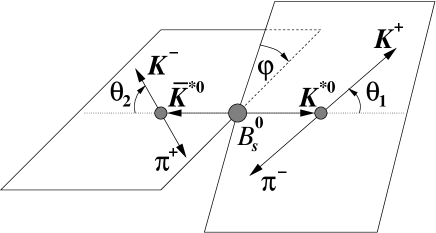
Figure 1: Definition of the angles involved in the analysis of ${{B}^{0}_{s}}\rightarrow{{K}^{*0}}{{\kern 1.99997pt\overline{\kern-1.99997ptK}{}}{}^{*0}}$ decays.

The decay rate of the $C\!P$-conjugated process, ${{\kern 1.79993pt\overline{\kern-1.79993ptB}{}}{}^{0}_{s}}\rightarrow(K^{-}\pi^{+})(K^{+}\pi^{-})$, can be obtained by exchanging each amplitude $A_{k}$ by $\eta_{k}\bar{A}_{k}$, where $\eta_{k}$ is the $C\!P$ eigenvalue of the final state described by $A_{k}$ [4]. In this paper, due to the limited size of the available data sample, no attempt is made to identify the flavour of the initial ${B}^{0}_{s}$ meson at production, thus suppressing the sensitivity to direct and mixing-induced $C\!P$ asymmetries. Nevertheless, $C\!P$ violation can still be studied through the measurement of triple product asymmetries and S–wave-induced direct $C\!P$ asymmetries.

2.2 Triple product asymmetries

Two TPs can be defined in $B$ meson decays into pairs of vector particles [5, 14, 4],

$$T_{1} = (\hat{n}_{V_{1}}\times\hat{n}_{V_{2}})\cdot\hat{p}_{V_{1}}=\sin\varphi\quad{\rm and}$$ (8)

$$T_{2} = 2(\hat{n}_{V_{1}}\cdot\hat{n}_{V_{2}})(\hat{n}_{V_{1}}\times\hat{n}_{V_{2}})\cdot\hat{p}_{V_{1}}=\sin 2\varphi,$$ (9)

where $\hat{n}_{V_{i}}$ ($i=1,2$) is a unit vector perpendicular to the $V_{i}$ decay plane and $\hat{p}_{V_{1}}$ is a unit vector in the direction of $V_{1}$ in the ${B}^{0}_{s}$ rest frame. The observable asymmetries associated with these TPs can be calculated from integrations of the differential decay rate as [14]

$$a_{T}^{1}(t) \equiv \frac{\Gamma(\cos\theta_{1}\cos\theta_{2}\sin\varphi>0,t)-\Gamma(\cos\theta_{1}\cos\theta_{2}\sin\varphi<0,t)}{\Gamma(\cos\theta_{1}\cos\theta_{2}\sin\varphi>0,t)+\Gamma(\cos\theta_{1}\cos\theta_{2}\sin\varphi<0,t)}\quad{\rm and}$$ (10)

$$a_{T}^{2}(t) \equiv \frac{\Gamma(\sin 2\varphi>0,t)-\Gamma(\sin 2\varphi<0,t)}{\Gamma(\sin 2\varphi>0,t)+\Gamma(\sin 2\varphi<0,t)}.$$ (11)

Nonzero TP asymmetries appear either due to a $T$-violating phase or a $T$-conserving phase in conjunction with final-state interactions.

When these asymmetries are measured in a sample where the production flavour is not identified, they become “true” $C\!P$-violating asymmetries, assuming that $C\!PT$ is conserved. This is manifest when $a_{T}^{1}$ and $a_{T}^{2}$ are written in terms of the amplitudes defining the decay rate in Eq. (5),

$$a_{T}^{1} = \frac{2\sqrt{2}}{\pi}\frac{1}{\mathcal{D}}\mathcal{I}m(\mathcal{A}_{\perp}\mathcal{A}_{0}^{*})\quad{\rm and}$$ (12)

$$a_{T}^{2} = -\frac{4}{\pi}\frac{1}{\mathcal{D}}\mathcal{I}m(\mathcal{A}_{\perp}\mathcal{A}_{\parallel}^{*}),$$ (13)

with $\mathcal{D}=|\mathcal{A}_{0}|^{2}+|\mathcal{A}_{\parallel}|^{2}+|\mathcal{A}_{\perp}|^{2}+|\mathcal{A}_{s}^{+}|^{2}+|\mathcal{A}_{s}^{-}|^{2}+|\mathcal{A}_{ss}|^{2}$. Taking into account these expressions and that the decay rate contribution associated with the $C\!P$-odd amplitude $\mathcal{A}_{\perp}$ changes sign under the $C\!P$ transformation, the asymmetries measured in the untagged sample, ${A}_{T}^{i}$, are proportional to the $C\!P$-violating interference terms $\mathcal{I}m(\mathcal{A}_{\perp}\mathcal{A}_{0,\parallel}^{*}-\bar{\mathcal{A}}_{\perp}\bar{\mathcal{A}}_{0,\parallel}^{*})$. Using Eq. (6), these terms can be written as

$$\mathcal{I}m(\mathcal{A}_{\perp}\mathcal{A}_{0,\parallel}^{*}-\bar{\mathcal{A}}_{\perp}\bar{\mathcal{A}}_{0,\parallel}^{*})=\frac{1}{2}e^{-\Gamma_{s}t}\bigg{[} \mathcal{I}m ({A}_{\perp}{A}_{0,\parallel}^{*}-\bar{{A}}_{\perp}\bar{{A}}_{0,\parallel}^{*}) \cosh \left(\frac{\Delta\Gamma_{s}}{2}t\right)$$

$$+ \mathcal{I}m [(\bar{{A}}_{\perp}{A}_{0,\parallel}^{*}+{A}_{\perp}^{*}\bar{{A}}_{0,\parallel})e^{-i\phi_{\rm mix}}] \sinh \left(\frac{\Delta\Gamma_{s}}{2}t\right)\bigg{]},$$ (14)

where $\Delta\Gamma_{s}\equiv\Gamma_{L}-\Gamma_{H}$, $\Gamma_{s}\equiv(\Gamma_{L}+\Gamma_{H})/{2}$ and $\phi_{\rm mix}$ is the phase in ${B}^{0}_{s}$–${\kern 1.79993pt\overline{\kern-1.79993ptB}{}}{}^{0}_{s}$ mixing. The coefficients $\mathcal{I}m({A}_{\perp}{A}_{0,\parallel}^{*}-\bar{{A}}_{\perp}\bar{{A}}_{0,\parallel}^{*})$ and $\mathcal{I}m[(\bar{{A}}_{\perp}{A}_{0,\parallel}^{*}+{A}_{\perp}^{*}\bar{{A}}_{0,\parallel})e^{-i\phi_{\rm mix}}]$ are TP and mixing-induced TP asymmetries, respectively, and are $C\!P$-violating quantities [4]. In the analysis presented in this paper, only the time-integrated asymmetries

$$A_{T}^{1} = \frac{2\sqrt{2}}{\pi}\frac{1}{{D}}\int\mathcal{I}m(\mathcal{A}_{\perp}\mathcal{A}_{0}^{*})\,{\rm d}t\quad{\rm and}$$ (15)

$$A_{T}^{2} = -\frac{4}{\pi}\frac{1}{{D}}\int\mathcal{I}m(\mathcal{A}_{\perp}\mathcal{A}_{\parallel}^{*})\,{\rm d}t,$$ (16)

are measured ($D=\int\mathcal{D}\,{\rm d}t$), with no identification of initial ${B}^{0}_{s}$ flavour. Thus $C\!P$-violating linear combinations of the above observables are accessible.

When the S–wave contribution is taken into account, two additional $C\!P$-even amplitudes, $\mathcal{A}_{s}^{-}$ and $\mathcal{A}_{ss}$, interfere with $\mathcal{A}_{\perp}$, and give rise to two additional $C\!P$-violating terms. Further asymmetric integrations of the decay rate, analogous to those in [14], lead to the following observables

$${A}_{T}^{3} \equiv\frac{\Gamma((\cos\theta_{1}+\cos\theta_{2})\sin\varphi>0)-\Gamma((\cos\theta_{1}+\cos\theta_{2})\sin\varphi<0)}{\Gamma((\cos\theta_{1}+\cos\theta_{2})\sin\varphi>0)+\Gamma((\cos\theta_{1}+\cos\theta_{2})\sin\varphi<0)}$$

$$=\frac{32}{5\pi\sqrt{3}}\frac{1}{\mathcal{D}}\int\mathcal{I}m\left(\left(\mathcal{A}_{\perp}\mathcal{A}_{s}^{-*}-\bar{\mathcal{A}}_{\perp}\bar{\mathcal{A}}_{s}^{-*}\right)\mathcal{M}_{1}(m)\mathcal{M}_{0}^{*}(m)\right)\mathrm{d}m$$ (17)

and

$${A}_{T}^{4} \equiv\frac{\Gamma(\sin\varphi>0)-\Gamma(\sin\varphi<0)}{\Gamma(\sin\varphi>0)+\Gamma(\sin\varphi<0)}$$

$$=\frac{3\pi}{4\sqrt{2}}\frac{1}{\mathcal{D}}\int\mathcal{I}m\left(\left(\mathcal{A}_{\perp}\mathcal{A}_{ss}^{*}-\bar{\mathcal{A}}_{\perp}\bar{\mathcal{A}}_{ss}^{*}\right)\mathcal{M}_{1}(m)\mathcal{M}_{0}^{*}(m)\right)\mathrm{d}m,$$ (18)

where the mass integration extends over the chosen $K\pi$ mass window. It is performed over the product of mass propagators of different resonances, times specific $C\!P$-violating observables involving $\mathcal{A}_{\perp}$.

Since $\mathcal{A}_{s}^{+}$ is also $C\!P$-odd, its interference terms with the $C\!P$-even amplitudes change sign under ${B}^{0}_{s}$ to ${\kern 1.79993pt\overline{\kern-1.79993ptB}{}}{}^{0}_{s}$ interchange. Consequently, four new $C\!P$-violating asymmetries are accessible from ${{B}^{0}_{s}}\rightarrow K^{+}\pi^{-}K^{-}\pi^{+}$ decays,

$${A}_{D}^{1} \equiv\frac{\Gamma(\cos\theta_{1}\cos\theta_{2}(\cos\theta_{1}-\cos\theta_{2})>0)-\Gamma(\cos\theta_{1}\cos\theta_{2}(\cos\theta_{1}-\cos\theta_{2})<0)}{\Gamma(\cos\theta_{1}\cos\theta_{2}(\cos\theta_{1}-\cos\theta_{2})>0)+\Gamma(\cos\theta_{1}\cos\theta_{2}(\cos\theta_{1}-\cos\theta_{2})<0)}$$

$$=\frac{\sqrt{2}}{5\sqrt{3}}\frac{1}{\mathcal{D}}\left[9\int\mathcal{R}e\left((\mathcal{A}_{s}^{+}\mathcal{A}_{0}^{*}-\bar{\mathcal{A}}_{s}^{+}\bar{\mathcal{A}}_{0}^{*})\mathcal{M}_{0}(m)\mathcal{M}_{1}^{*}(m)\right)\mathrm{d}m\right.$$

$$\left.\ \ \ \ \ \ \ \ \ \ \ \ +5\int\mathcal{R}e\left((\mathcal{A}_{s}^{+}\mathcal{A}_{ss}^{*}-\bar{\mathcal{A}}_{s}^{+}\bar{\mathcal{A}}_{ss}^{*})\mathcal{M}_{1}(m)\mathcal{M}_{0}^{*}(m)\right)\mathrm{d}m\right],$$ (19)

$${A}_{D}^{2} \equiv\frac{\Gamma((\cos\theta_{1}-\cos\theta_{2})\cos\varphi>0)-\Gamma((\cos\theta_{1}-\cos\theta_{2})\cos\varphi<0)}{\Gamma((\cos\theta_{1}-\cos\theta_{2})\cos\varphi>0)+\Gamma((\cos\theta_{1}-\cos\theta_{2})\cos\varphi<0)}$$

$$=-\frac{32}{5\pi\sqrt{3}}\frac{1}{\mathcal{D}}\int\mathcal{R}e\left((\mathcal{A}_{s}^{+}\mathcal{A}_{\parallel}^{*}-\bar{\mathcal{A}}_{s}^{+}\bar{\mathcal{A}}_{\parallel}^{*})\mathcal{M}_{0}(m)\mathcal{M}_{1}^{*}(m)\right)\mathrm{d}m,$$ (20)

$${A}_{D}^{3} \equiv\frac{\Gamma((\cos\theta_{1}-\cos\theta_{2})>0)-\Gamma((\cos\theta_{1}-\cos\theta_{2})<0)}{\Gamma((\cos\theta_{1}-\cos\theta_{2})>0)+\Gamma((\cos\theta_{1}-\cos\theta_{2})<0)}$$

$$=\frac{2\sqrt{2}}{5\sqrt{3}}\frac{1}{\mathcal{D}}\left[3\int\mathcal{R}e\left((\mathcal{A}_{s}^{+}\mathcal{A}_{0}^{*}-\bar{\mathcal{A}}_{s}^{+}\bar{\mathcal{A}}_{0}^{*})\mathcal{M}_{0}(m)\mathcal{M}_{1}^{*}(m)\right)\mathrm{d}m\right.$$

$$\left.\ \ \ \ \ \ \ \ \ \ \ \ +5\int\mathcal{R}e\left((\mathcal{A}_{s}^{+}\mathcal{A}_{ss}^{*}-\bar{\mathcal{A}}_{s}^{+}\bar{\mathcal{A}}_{ss}^{*})\mathcal{M}_{1}(m)\mathcal{M}_{0}^{*}(m)\right)\mathrm{d}m\right]$$ (21)

and

$${A}_{D}^{4} \equiv\frac{\Gamma((\cos^{2}\theta_{1}-\cos^{2}\theta_{2})>0)-\Gamma((\cos^{2}\theta_{1}-\cos^{2}\theta_{2})<0)}{\Gamma((\cos^{2}\theta_{1}-\cos^{2}\theta_{2})>0)+\Gamma((\cos^{2}\theta_{1}-\cos^{2}\theta_{2})<0)}$$

$$=\frac{1}{\mathcal{D}}\mathcal{R}e\left(\mathcal{A}_{s}^{+}\mathcal{A}_{s}^{-*}-\bar{\mathcal{A}}_{s}^{+}\bar{\mathcal{A}}_{s}^{-*}\right).$$ (22)

Some of these terms have the form $\mathcal{R}e(\mathcal{A}_{s}^{+}\mathcal{A}_{k}^{*}-\bar{\mathcal{A}}_{s}^{+}\bar{\mathcal{A}}_{k}^{*})$, with $k=0,\parallel,s^{-},ss$, which is characteristic of direct $C\!P$ asymmetries.

As shown above, TP and several direct $C\!P$ asymmetries are accessible from untagged ${{B}^{0}_{s}}\rightarrow{{K}^{*0}}{{\kern 1.99997pt\overline{\kern-1.99997ptK}{}}{}^{*0}}$ decays, provided that a scalar $K\pi$ background component is present. These $C\!P$-violating observables are sensitive to the contributions of FCNC processes induced by neutral scalars, which are present, for example, in models with an extended Higgs sector. Constraints on possible FCNC couplings of Higgs scalars have been recently examined [15, 16]. Non-zero values of $A_{T}^{i}$ or $A_{D}^{i}$ would allow the characterisation of those operators contributing to the effective Hamiltonian. In particular an enhanced contribution from $A_{D}^{1,2,3}$ with respect to the other observables, would reveal stronger $(V-A)\times(V+A)$ ($LR$) and $(V+A)\times(V-A)$ ($RL$) components with respect to $RR$ and $LL$ operators in the above models [4].

2.3 Angular analysis

Assuming that no $C\!P$ violation arises in this decay, an angular analysis of the decay products determines the polarisation fractions of the ${{B}^{0}_{s}}\rightarrow{{K}^{*0}}{{\kern 1.99997pt\overline{\kern-1.99997ptK}{}}{}^{*0}}$ decay and the contribution of the various S–wave amplitudes. The time-integrated decay rate can be expressed as

$$\frac{{\rm d}^{5}\Gamma}{{\rm d}\Omega\,{\rm d}m_{1}\,{\rm d}m_{2}}=\hat{N}\sum_{n=1}^{21}K_{n}(m_{1},m_{2})F_{n}(\Omega),$$ (23)

where the functions $K_{n}$ contain the dependence on the amplitudes entering the decay, with their corresponding mass propagators, and $\hat{N}$ is an overall normalisation constant. The $K_{n}$ functions are given in Table 1 together with the decay angle functions $F_{n}$. All terms proportional to the TP and S–wave-induced $C\!P$ asymmetries ($n=5,6,21$ and the symmetric $A_{s}^{+}\leftrightarrow A_{s}^{-}$ terms in $n=8-11,13-16$) cancel under the assumption of $C\!P$ conservation.

Table 1: Untagged time-integrated terms used in the analysis, under the assumption of no $C\!P$ violation.

$n$	$K_{n}$	$F_{n}$
1	$\frac{1}{\Gamma_{L}}{|A_{0}|}^{2}|\mathcal{M}_{1}(m_{1})|^{2}|\mathcal{M}_{1}(m_{2})|^{2}$	$\cos^{2}\theta_{1}\cos^{2}\theta_{2}$
2	$\frac{1}{\Gamma_{L}}{|A_{\parallel}|}^{2}|\mathcal{M}_{1}(m_{1})|^{2}|\mathcal{M}_{1}(m_{2})|^{2}$	$\frac{1}{2}\sin^{2}\theta_{1}\sin^{2}\theta_{2}\cos^{2}\varphi$
3	$\frac{1}{\Gamma_{H}}{|A_{\perp}|}^{2}|\mathcal{M}_{1}(m_{1})|^{2}|\mathcal{M}_{1}(m_{2})|^{2}$	$\frac{1}{2}\sin^{2}\theta_{1}\sin^{2}\theta_{2}\sin^{2}\varphi$
4	$\frac{1}{\Gamma_{L}}{|A_{\parallel}||A_{0}|}\cos{\delta_{\parallel}}|\mathcal{M}_{1}(m_{1})|^{2}|\mathcal{M}_{1}(m_{2})|^{2}$	$\frac{1}{2\sqrt{2}}\sin 2\theta_{1}\sin 2\theta_{2}\cos\varphi$
5	$0$	$-\frac{1}{2\sqrt{2}}\sin 2\theta_{1}\sin 2\theta_{2}\sin\varphi$
6	$0$	$-\frac{1}{2}\sin^{2}\theta_{1}\sin^{2}\theta_{2}\sin 2\varphi$
7	$\frac{1}{2}(\frac{{|A_{s}^{+}|}^{2}}{\Gamma_{H}}+\frac{{|A_{s}^{-}|}^{2}}{\Gamma_{L}})|\mathcal{M}_{1}(m_{1})|^{2}|\mathcal{M}_{0}(m_{2})|^{2}$	$\frac{1}{3}\cos^{2}\theta_{1}$
8	$\frac{1}{\sqrt{2}}\frac{1}{\Gamma_{L}}{|A_{s}^{-}|}{|A_{0}|}\mathcal{R}e(e^{i{\delta_{s}^{-}}}\mathcal{M}_{1}^{*}(m_{2})\mathcal{M}_{0}(m_{2}))|\mathcal{M}_{1}(m_{1})|^{2}$	$-\frac{2}{\sqrt{3}}\cos^{2}\theta_{1}\cos\theta_{2}$
9	$\frac{1}{\sqrt{2}}\frac{1}{\Gamma_{L}}{|A_{s}^{-}|}{|A_{\parallel}|}\mathcal{R}e(e^{i({\delta_{s}^{-}}-{\delta_{\parallel}})}\mathcal{M}_{1}^{*}(m_{2})\mathcal{M}_{0}(m_{2}))|\mathcal{M}_{1}(m_{1})|^{2}$	$-\frac{1}{\sqrt{6}}\sin 2\theta_{1}\sin\theta_{2}\cos\varphi$
10	$\frac{1}{\sqrt{2}}\frac{1}{\Gamma_{H}}{|A_{s}^{+}|}{|A_{\perp}|}\mathcal{I}m(e^{i({\delta_{\perp}}-{\delta_{s}^{+}})}\mathcal{M}_{0}^{*}(m_{2})\mathcal{M}_{0}(m_{2}))|\mathcal{M}_{1}(m_{1})|^{2}$	$\frac{1}{\sqrt{6}}\sin 2\theta_{1}\sin\theta_{2}\sin\varphi$
11	$\frac{1}{\sqrt{2}}\frac{1}{\Gamma_{L}}{|A_{s}^{-}|}{|A_{ss}|}\mathcal{R}e(e^{i({\delta_{s}^{-}}-{\delta_{ss}})}\mathcal{M}_{0}^{*}(m_{1})\mathcal{M}_{1}(m_{1}))|\mathcal{M}_{0}(m_{2})|^{2}$	$\frac{2}{3\sqrt{3}}\cos\theta_{1}$
12	$\frac{1}{2}(\frac{{|A_{s}^{+}|}^{2}}{\Gamma_{H}}+\frac{{|A_{s}^{-}|}^{2}}{\Gamma_{L}})|\mathcal{M}_{0}(m_{1})|^{2}|\mathcal{M}_{1}(m_{2})|^{2}$	$\frac{1}{3}\cos^{2}\theta_{2}$
13	$-\frac{1}{\sqrt{2}}\frac{1}{\Gamma_{L}}{|A_{s}^{-}|}{|A_{0}|}\mathcal{R}e(e^{i{\delta_{s}^{-}}}\mathcal{M}_{1}^{*}(m_{1})\mathcal{M}_{0}(m_{1}))|\mathcal{M}_{1}(m_{2})|^{2}$	$\frac{2}{\sqrt{3}}\cos\theta_{1}\cos^{2}\theta_{2}$
14	$-\frac{1}{\sqrt{2}}\frac{1}{\Gamma_{L}}{|A_{s}^{-}|}{|A_{\parallel}|}\mathcal{R}e(e^{i({\delta_{s}^{-}}-{\delta_{\parallel}})}\mathcal{M}_{1}^{*}(m_{1})\mathcal{M}_{0}(m_{1}))|\mathcal{M}_{1}(m_{2})|^{2}$	$\frac{1}{\sqrt{6}}\sin\theta_{1}\sin 2\theta_{2}\cos\varphi$
15	$\frac{1}{\sqrt{2}}\frac{1}{\Gamma_{H}}{|A_{s}^{+}|}{|A_{\perp}|}\mathcal{I}m(e^{i({\delta_{\perp}}-{\delta_{s}^{+}})}\mathcal{M}_{0}^{*}(m_{1})\mathcal{M}_{0}(m_{1}))|\mathcal{M}_{1}(m_{2})|^{2}$	$-\frac{1}{\sqrt{6}}\sin\theta_{1}\sin 2\theta_{2}\sin\varphi$
16	$-\frac{1}{\sqrt{2}}\frac{1}{\Gamma_{L}}{|A_{s}^{-}|}{|A_{ss}|}\mathcal{R}e(e^{i({\delta_{s}^{-}}-{\delta_{ss}})}\mathcal{M}_{0}^{*}(m_{2})\mathcal{M}_{1}(m_{2}))|\mathcal{M}_{0}(m_{1})|^{2}$	$-\frac{2}{3\sqrt{3}}\cos\theta_{2}$
17	$(\frac{{|A_{s}^{+}|}^{2}}{\Gamma_{H}}-\frac{{|A_{s}^{-}|}^{2}}{\Gamma_{L}})\mathcal{R}e(\mathcal{M}^{*}_{1}(m_{1})\mathcal{M}^{*}_{0}(m_{2})\mathcal{M}_{0}(m_{1})\mathcal{M}_{1}(m_{2}))$	$-\frac{1}{3}\cos\theta_{1}\cos\theta_{2}$
18	$\frac{1}{\Gamma_{L}}{|A_{ss}|}^{2}|\mathcal{M}_{0}(m_{1})|^{2}|\mathcal{M}_{0}(m_{2})|^{2}$	$\frac{1}{9}$
19	$\frac{1}{\Gamma_{L}}{|A_{ss}|}{|A_{0}|}\mathcal{R}e(e^{i{\delta_{ss}}}\mathcal{M}_{1}^{*}(m_{1})\mathcal{M}_{1}^{*}(m_{2})\mathcal{M}_{0}(m_{1})\mathcal{M}_{0}(m_{2}))$	$-\frac{2}{3}\cos\theta_{1}\cos\theta_{2}$
20	$\frac{1}{\Gamma_{L}}{|A_{ss}|}{|A_{\parallel}|}\mathcal{R}e(e^{i({\delta_{ss}}-{\delta_{\parallel}})}\mathcal{M}_{1}^{*}(m_{1})\mathcal{M}_{1}^{*}(m_{2})\mathcal{M}_{0}(m_{1})\mathcal{M}_{0}(m_{2}))$	$-\frac{\sqrt{2}}{3}\sin\theta_{1}\sin\theta_{2}\cos\varphi$
21	$0$	$\frac{\sqrt{2}}{3}\sin\theta_{1}\sin\theta_{2}\sin\varphi$

The dependence of each amplitude on the invariant mass of the $K^{+}\pi^{-}$ and $K^{-}\pi^{+}$ pairs is given by the propagators $\mathcal{M}_{J}(m)\propto\mathcal{R}_{J}(m)\times m/q$, where $q$ is the momentum of each meson in the rest frame of the $K\pi$ pair

$$q=\frac{\sqrt{(m^{2}-(M_{\pi}+M_{K})^{2})(m^{2}-(M_{\pi}-M_{K})^{2}})}{2m}.$$ (24)

The P–wave propagator, $J=1$, is parameterised using a spin-1 relativistic Breit-Wigner resonance function

$$\mathcal{R}_{1}(m)=\frac{M_{1}\Gamma_{1}(m)}{(M_{1}^{2}-m^{2})-iM_{1}\Gamma_{1}(m)}.$$ (25)

The mass-dependent width is given by

$$\Gamma_{1}(m)=\Gamma_{1}\frac{M_{1}}{m}\frac{1+r^{2}q_{1}^{2}}{1+r^{2}q^{2}}\left(\frac{q}{q_{1}}\right)^{3},$$ (26)

where $M_{1}$ and $\Gamma_{1}$ are the ${{K}^{*0}}(892)$ resonance mass and width, $r$ is the interaction radius and $q_{1}$ corresponds to Eq. (24) evaluated at the resonance position ($M_{1}$).

To describe the S–wave propagator, $\mathcal{M}_{0}(m)$, the LASS parameterisation [17] is used, which is an effective-range elastic scattering amplitude, interfering with the ${{K}^{*}_{0}}(1430)$ resonance,

$$\mathcal{R}_{0}(m)\propto\frac{1}{\cot\delta_{\beta}-i}+e^{2i\delta_{\beta}}\frac{M_{0}\Gamma_{0}(m)}{M_{0}^{2}-m^{2}-iM_{0}\Gamma_{0}(m)},$$ (27)

where

$$\Gamma_{0}(m)=\Gamma_{0}\frac{M_{0}}{m}\left(\frac{q}{q_{0}}\right),$$ (28)

and the non-resonant component is described as

$$\cot\delta_{\beta}=\frac{1}{aq}+\frac{1}{2}bq.$$ (29)

The values of the mass propagator parameters, including the resonance masses and widths, $M_{J}$ and $\Gamma_{J}$, and the the scattering length ($a$) and effective range ($b$), are summarized in Table 2. Other shapes modelling the S–wave propagator, including an explicit Breit-Wigner contribution for the ${{K}^{*}_{0}}(800)$ resonance, are considered in the systematic uncertainties.

The normalisation of the mass propagators

$$\int|\mathcal{M}_{0}|^{2}\mathrm{d}m=\int|\mathcal{M}_{1}|^{2}\mathrm{d}m=1$$ (30)

in the mass range considered, together with the normalisation condition

$$|A_{0}|^{2}+|A_{\parallel}|^{2}+|A_{\perp}|^{2}+|A_{s}^{+}|^{2}+|A_{s}^{-}|^{2}+|A_{ss}|^{2}=1,$$ (31)

guarantees the definition of the squared amplitudes as fractions of different partial waves. The polarisation fractions for the vector mode, ${{B}^{0}_{s}}\rightarrow{{K}^{*0}}{{\kern 1.99997pt\overline{\kern-1.99997ptK}{}}{}^{*0}}$, are defined as

$$f_{L,\parallel,\perp}=\frac{|A_{0,\parallel,\perp}|^{2}}{|A_{0}|^{2}+|A_{\parallel}|^{2}+|A_{\perp}|^{2}}\,.$$ (32)

The overall phase of the propagators is defined such that

$$\arg[\mathcal{M}_{0}(M_{1})]=\arg[\mathcal{M}_{1}(M_{1})]=0$$ (33)

and the convention $\delta_{0}\equiv\arg(A_{0})=0$ is adopted. Therefore $\delta_{\parallel}$, $\delta_{\perp}$, $\delta_{s}^{-}$, $\delta_{s}^{+}$ and $\delta_{ss}$ are defined as the phase difference between the corresponding amplitude and $A_{0}$ at the ${K}^{*0}$ mass pole. As a consequence of the lack of initial ${B}^{0}_{s}$ or ${\kern 1.79993pt\overline{\kern-1.79993ptB}{}}{}^{0}_{s}$ flavour information, the phases $\delta_{\perp}$ and $\delta_{s}^{+}$ can not be measured independently, and only their difference is accessible to this analysis.

Table 2: Parameters of the mass propagators used in the fit.

	$(K\pi)_{0}^{*0}$	$K^{*}(892)^{0}$
	$J=0$ [17, 18]	$J=1$ [19]
$M_{J}$ (${\mathrm{\,Me\kern-1.00006ptV\!/}c^{2}}$)	$1435\pm 5\pm\phantom{1}5$	$895.81\pm 0.19$
$\Gamma_{J}$ (${\mathrm{\,Me\kern-1.00006ptV\!/}c^{2}}$)	$\phantom{1}279\pm 6\pm 21$	$\phantom{0}47.4\phantom{1}\pm 0.6\phantom{0}$
$r$ ($\mathrm{\,Ge\kern-1.00006ptV}^{-1}$)	-	$\phantom{00}3.0\phantom{1}\pm 0.5\phantom{0}$
$a$ ($\mathrm{\,Ge\kern-1.00006ptV}^{-1}$)	$1.95\pm 0.09\pm 0.06$	-
$b$ ($\mathrm{\,Ge\kern-1.00006ptV}^{-1}$)	$1.76\pm 0.36\pm 0.67$	-

3 The LHCb detector

The LHCb detector [20, 21] is a single-arm forward spectrometer covering the pseudorapidity range $2<\eta<5$, designed for the study of particles containing $b$ or $c$ quarks. The detector includes a high-precision tracking system consisting of a silicon-strip vertex detector surrounding the $pp$ interaction region, a large-area silicon-strip detector located upstream of a dipole magnet with a bending power of about $4{\rm\,Tm}$, and three stations of silicon-strip detectors and straw drift tubes placed downstream of the magnet. The tracking system provides a measurement of momentum, $p$, of charged particles with a relative uncertainty that varies from 0.5% at low momentum to 1.0% at 200${\mathrm{\,Ge\kern-1.00006ptV\!/}c}$. The minimum distance of a track to a primary vertex, the impact parameter (IP), is measured with a resolution of $(15+29/\mbox{$p_{\rm T}$}){\,\upmu\rm m}$, where $p_{\rm T}$ is the component of the momentum transverse to the beam, in ${\mathrm{\,Ge\kern-1.00006ptV\!/}c}$. Different types of charged hadrons are distinguished using information from two ring-imaging Cherenkov detectors. Photons, electrons and hadrons are identified by a calorimeter system consisting of scintillating-pad and preshower detectors, an electromagnetic calorimeter and a hadronic calorimeter. Muons are identified by a system composed of alternating layers of iron and multiwire proportional chambers. The online event selection is performed by a trigger, which consists of a hardware stage, based on information from the calorimeter and muon systems, followed by a software stage, which applies a full event reconstruction.

In the analysis presented here, all hardware triggers are used. The software trigger requires a multi-track secondary vertex with a significant displacement from the primary $pp$ interaction vertices (PVs). At least one charged particle must have a transverse momentum $\mbox{$p_{\rm T}$}>1.7{\mathrm{\,Ge\kern-1.00006ptV\!/}c}$ and be inconsistent with originating from a PV. A multivariate algorithm [22] identifies secondary vertices consistent with the decay of a $b$ hadron.

Simulated ${{B}^{0}_{s}}\rightarrow{{K}^{*0}}{{\kern 1.99997pt\overline{\kern-1.99997ptK}{}}{}^{*0}}$ events are used to characterise the detector response to signal events. In the simulation, $pp$ collisions are generated using Pythia [23] with a specific LHCb configuration [24]. Decays of hadronic particles are described by EvtGen [25], in which final-state radiation is generated using Photos [26]. The interaction of the generated particles with the detector and its response are implemented using the Geant4 toolkit [27, *Agostinelli:2002hh] as described in Ref. [29].

4 Event selection and signal yield

The event selection is similar to that used in the previous analysis [8]. ${K}^{*0}$ candidates are formed from two high-quality oppositely charged tracks identified as a kaon and pion, respectively. They are selected to have $\mbox{$p_{\rm T}$}>500$${\mathrm{\,Me\kern-1.00006ptV\!/}c}$ and to be displaced from any PV. The $K^{+}\pi^{-}$ and $K^{-}\pi^{+}$ pairs are required to have invariant mass within $\pm 150$${\mathrm{\,Me\kern-1.00006ptV\!/}c^{2}}$ of the known ${K}^{*0}$ mass, which corresponds to 74% of the total phase-space for ${{B}^{0}_{s}}\rightarrow{{K}^{*0}}{{\kern 1.99997pt\overline{\kern-1.99997ptK}{}}{}^{*0}}$, and $\mbox{$p_{\rm T}$}>900$${\mathrm{\,Me\kern-1.00006ptV\!/}c}$. Each ${B}^{0}_{s}$ candidate is constructed by combining a ${K}^{*0}$ and ${\kern 1.99997pt\overline{\kern-1.99997ptK}{}}{}^{*0}$, requiring the four tracks to form a good vertex well-separated from any PV. The ${B}^{0}_{s}$ candidate invariant mass is restricted to be within the interval $[5100,5866]$${\mathrm{\,Me\kern-1.00006ptV\!/}c^{2}}$ and its momentum vector is required to point towards one PV.

In order to further discriminate the ${{B}^{0}_{s}}\rightarrow{{K}^{*0}}{{\kern 1.99997pt\overline{\kern-1.99997ptK}{}}{}^{*0}}$ signal from the combinatorial background, different properties of the decay are combined into a multivariate discriminator [30]. The variables combined in the discriminator are the ${B}^{0}_{s}$ candidate IP with respect to the associated PV, its lifetime and $p_{\rm T}$, the minimum $\chi^{2}_{\rm IP}$ of the four daughter tracks (defined as the difference between the $\chi^{2}$ of a PV formed with and without the particle in question) with respect to the same PV and the distance of closest approach between the two ${K}^{*0}$ candidates. The discriminator is trained using simulated ${{B}^{0}_{s}}\rightarrow{{K}^{*0}}{{\kern 1.99997pt\overline{\kern-1.99997ptK}{}}{}^{*0}}$ events for signal and a small data sample excluded from the rest of the analysis as background. The optimal discriminator requirement is determined by maximising the figure of merit $N_{S}/\sqrt{N_{S}+N_{B}}$ in a test sample containing signal ($S$) and background ($B$) events of the same nature as those used in the training sample.

Differences in the log-likelihood for various particle identification hypotheses (${\Delta\ln\mathcal{L}}_{a-b}$) are used to minimise the contamination from specific $B$ decays. Contributions from ${{B}^{0}}\rightarrow\rho{{\kern 1.99997pt\overline{\kern-1.99997ptK}{}}{}^{*0}}$ and ${{B}^{0}}\rightarrow\phi{{K}^{*0}}$ modes are reduced by the ${\Delta\ln\mathcal{L}}_{K-\pi}$ requirements of kaons and pions. A small contamination from $\Lambda^{0}_{b}\rightarrow p\pi^{-}K^{-}\pi^{+}$ decays is observed and suppressed with ${\Delta\ln\mathcal{L}}_{{p}-K}$ requirements.

An extended unbinned maximum likelihood fit to the mass spectrum of the selected ${{B}^{0}_{s}}\rightarrow K^{+}\pi^{-}K^{-}\pi^{+}$ candidates is performed. The signal is modelled by a sum of two Crystal Ball distributions [31] that share common mean and width. The same distribution is used to describe the ${B}^{0}$ decay into the same final state. Components for ${{B}^{0}}\rightarrow\phi{{K}^{*0}}$ and $\Lambda^{0}_{b}\rightarrow p\pi^{-}K^{-}\pi^{+}$ decays are included in the fit with shapes extracted from simulated events. The contribution from ${{B}^{0}}\rightarrow\rho{{\kern 1.99997pt\overline{\kern-1.99997ptK}{}}{}^{*0}}$ decays is estimated to be negligible from simulation studies. Finally, partially reconstructed $B$ decays are parameterised using an ARGUS distribution [32] and the remaining combinatorial background is modelled using an exponential function. The fit result is shown in Fig. 2. A total of $697\pm 31$ ${{B}^{0}_{s}}\rightarrow K^{+}\pi^{-}K^{-}\pi^{+}$ decays is obtained.

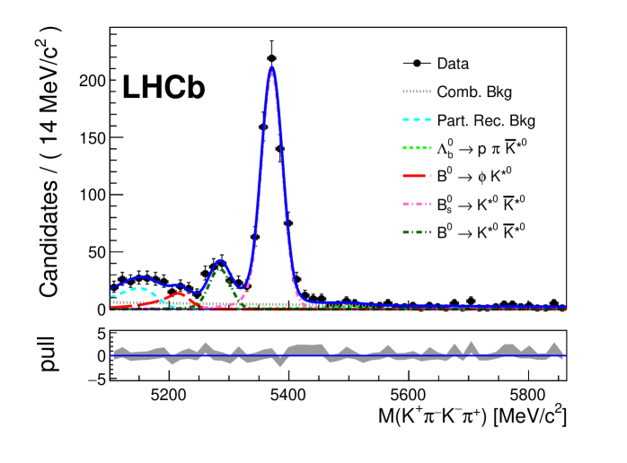
Figure 2: Invariant mass distribution for selected $K^{+}\pi^{-}K^{-}\pi^{+}$ candidates. The (blue) solid line is the result of the fit explained in the text. The ${B}^{0}_{s}$ and ${B}^{0}$ signal peaks are shown as as dashed-dotted lines (pink and dark green, respectively). The various peaking background components are represented as dotted lines: (red) ${{B}^{0}}\rightarrow\phi{{K}^{*0}}$, (green) $\Lambda^{0}_{b}\rightarrow p\pi^{-}K^{-}\pi^{+}$ and (light blue) partially reconstructed decays. The (grey) dotted line is the combinatorial background component. The normalised residual (pull) is shown below.

4.1 Acceptance properties

Effects introduced in data due to the geometry of the detector and to the selection requirements need to be taken into account in the measurement.

The study of simulated ${{B}^{0}_{s}}\rightarrow{{K}^{*0}}{{\kern 1.99997pt\overline{\kern-1.99997ptK}{}}{}^{*0}}$ events shows that the detection and selection efficiency is not uniform as a function of the decay angles $\theta_{1}$ and $\theta_{2}$, but has no dependence, at the level of precision needed for this analysis, on $\varphi$ and on the invariant mass of the two $K\pi$ pairs, $m_{1}$ and $m_{2}$. The acceptance decreases as $\cos\theta_{i}$ approaches 1. This feature is mainly induced by the requirement on the minimum $p_{\rm T}$ of the daughter pions. This effect is modelled by a two-dimensional function in $\cos\theta_{1}$ and $\cos\theta_{2}$, which is extracted from simulation.

Since the trigger system uses the $p_{\rm T}$ of the charged particles, the acceptance effect is different for events where signal tracks were involved in the trigger decision (called trigger-on-signal or TOS throughout) and those where the trigger decision was made using information from the rest of the event (non-TOS). The data set is split according to these two categories and a different acceptance correction is applied to each subset.

5 Triple product and direct $\mathbf{CP}$ asymmetries

Triple products and direct $C\!P$ asymmetries are calculated for ${{B}^{0}_{s}}\rightarrow K^{+}\pi^{-}K^{-}\pi^{+}$ using Eqs. (10) and (11), after time integration, and Eqs. (17)–(22) from those candidates with a four-body invariant mass within $\pm 30$ ${\mathrm{\,Me\kern-1.00006ptV\!/}c^{2}}$ of the known ${B}^{0}_{s}$ mass. The background in this interval, which is purely combinatorial, is subtracted according to the fraction calculated from the result of the invariant mass fit, $f_{\rm bkg}=(3.44\pm 0.34)\%$. The angular distributions of the background are extracted from the upper mass sideband, defined by $M(K^{+}\pi^{-}K^{-}\pi^{+})>5550$ ${\mathrm{\,Me\kern-1.00006ptV\!/}c^{2}}$. Acceptance effects are then corrected in the signal angular distributions. The measured asymmetries are listed in Table 3. From the definitions given in Sect. 2.2, correlations of the order of 5% are expected among these asymmetries, with the exception of $A_{D}^{1}$ and $A_{D}^{3}$ where the correlation is calculated to be close to 90%.

Table 3: Triple product and direct $C\!P$ asymmetries measured in this analysis. The first uncertainties are statistical and the second systematic.

Asymmetry	Value
$A_{T}^{1}$	$\phantom{-}0.003$ $\pm$ 0.041 $\pm$ 0.009
$A_{T}^{2}$	$\phantom{-}0.009$ $\pm$ 0.041 $\pm$ 0.009
$A_{T}^{3}$	$\phantom{-}0.019$ $\pm$ 0.041 $\pm$ 0.008
$A_{T}^{4}$	$-0.040$ $\pm$ 0.041 $\pm$ 0.008
$A_{D}^{1}$	$-0.061$ $\pm$ 0.041 $\pm$ 0.012
$A_{D}^{2}$	$\phantom{-}0.081$ $\pm$ 0.041 $\pm$ 0.008
$A_{D}^{3}$	$-0.079$ $\pm$ 0.041 $\pm$ 0.023
$A_{D}^{4}$	$-0.081$ $\pm$ 0.041 $\pm$ 0.010

The main systematic uncertainty in these measurements is associated to the angular acceptance correction. Discrepancies in the $p_{\rm T}$ spectra and the particle identification efficiencies between data and simulation are used to modify the acceptance function obtained from simulation. Systematic uncertainties are determined from the variation in the measured asymmetries when this modified acceptance is used. Systematic effects are found to be larger in case of the four direct $C\!P$ asymmetries, in particular for $A_{D}^{3}$, which has a strong dependence on $\cos\theta_{1,2}$. In addition, the lifetime-biasing selection criteria have a slightly different effect on the various amplitudes, which correspond to decays with different effective lifetimes, due to the width difference between ${B}^{0}_{s}$ mass eigenstates [33, 34]. This could induce a bias in the measured TP and direct $C\!P$ asymmetries. A set of simulated experiments is performed to estimate the impact of the lifetime acceptance in the eight quantities. The observed deviations are small and are used to assign a systematic uncertainty. Finally, the effect of the uncertainty in the background contribution is estimated by changing the background fraction and the parameters in the background model within their statistical uncertainty and recalculating the asymmetries.

6 Angular analysis

The magnitudes and phases of the various amplitudes contributing to the ${{B}^{0}_{s}}\rightarrow K^{+}\pi^{-}K^{-}\pi^{+}$ decay are determined using a five-dimensional fit to the three helicity angles ($\Omega$) and to the invariant mass of the two $K{\pi}$ pairs ($m_{1},m_{2}$) of all candidates with a four-body invariant mass $|M(K^{+},\pi^{-},K^{-},\pi^{+})-m_{{{B}^{0}_{s}}}|<30{\mathrm{\,Me\kern-1.00006ptV\!/}c^{2}}$.

The model used to describe the distribution in these five variables is given by

$$\mathcal{F}(\Omega,m_{1},m_{2})=(1-f_{\rm bkg})F(\Omega,m_{1},m_{2})\times\varepsilon(\Omega)+f_{\rm bkg}F_{\rm bkg}(\Omega,m_{1},m_{2}),$$ (34)

where $F(\Omega,m_{1},m_{2})$ is the probability density function in Eq. (5), $\varepsilon(\Omega)$ is the acceptance function modelling the effects introduced by reconstruction, selection and trigger reported in Sect. 4.1, and $F_{\rm bkg}(\Omega,m_{1},m_{2})$ describes the distribution of the background extracted from the upper mass sideband. The background fraction, $f_{\rm bkg}$, is obtained from the result of the fit to the invariant mass of the ${B}^{0}_{s}$ candidates.

Using this model, an unbinned maximun likelihood fit is performed simultaneously for TOS and non-TOS ${{B}^{0}_{s}}\rightarrow K^{+}\pi^{-}K^{-}\pi^{+}$ candidates, where only the acceptance function and the background fraction are different between the two samples. The results of the fit are summarised in Table 4. Figures 3 and 4 show the angular and $K\pi$ mass projections of the multi-dimensional distributions. To quantitatively demonstrate the interference between the different partial waves, a forward-backward asymmetry is defined for ${K}^{*0}$ meson as $A_{\rm FB}=(N_{\rm F}-N_{\rm B})/(N_{\rm F}+N_{\rm B})$, where $N_{\rm F}$ ($N_{\rm B}$) is the number of $K^{+}$ mesons emitted with positive (negative) $\cos\theta_{1}$, and analogously for the ${\kern 1.99997pt\overline{\kern-1.99997ptK}{}}{}^{*0}$ meson. Their evolution with the $K\pi$ invariant mass is shown in Fig. 4, as an additonal projection of the fit result. According to Eq. (5) these asymmetries are proportional to the interference term between $A_{s}^{-}$ and $A_{0}$.

Figure 5 shows the likelihood for the longitudinal polarisation fraction $f_{L}$, where all the other parameters are minimised at each point of the curve, depicting parabolic behaviour around the minimum. Additionally, confidence regions in the $|A_{s}^{-}|^{2}$–$f_{L}$ plane are shown.

Table 4: Results of the simultaneous fit to ${{B}^{0}_{s}}\rightarrow K^{+}\pi^{-}K^{-}\pi^{+}$ TOS and non-TOS candidates with $|M(K^{+},\pi^{-},K^{-},\pi^{+})-m_{{{B}^{0}_{s}}}|<30{\mathrm{\,Me\kern-1.00006ptV\!/}c^{2}}$ (phases are measured in radians). The first uncertainties are statistical and the second systematic.

Parameter	Value
$f_{L}$	$0.201\pm 0.057\pm 0.040$
$f_{\parallel}$	$0.215\pm 0.046\pm 0.015$
$|A_{s}^{+}|^{2}$	$0.114\pm 0.037\pm 0.023$
$|A_{s}^{-}|^{2}$	$0.485\pm 0.051\pm 0.019$
$|A_{ss}|^{2}$	$0.066\pm 0.022\pm 0.007$
$\delta_{\parallel}$	$5.31\pm 0.24\pm 0.14$
$\delta_{\perp}-\delta_{s}^{+}$	$1.95\pm 0.21\pm 0.04$
$\delta_{s}^{-}$	$1.79\pm 0.19\pm 0.19$
$\delta_{ss}$	$1.06\pm 0.27\pm 0.23$

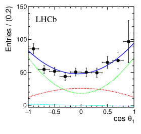
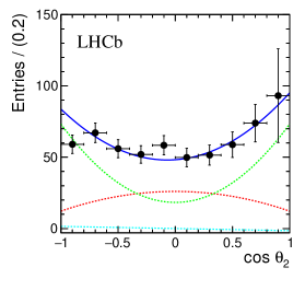
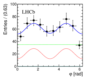
Figure 3: Results of the simultaneous fit to ${{B}^{0}_{s}}\rightarrow K^{+}\pi^{-}K^{-}\pi^{+}$ candidates (blue solid line) in the three helicity angles. The dots represent the data after background subtraction and acceptance correction. The red dashed line is the P–wave component, the green dashed line is the S–wave component and the light-blue dashed line represents the $\mathcal{A}^{+}_{s}\mathcal{A}_{0}$ interference term.

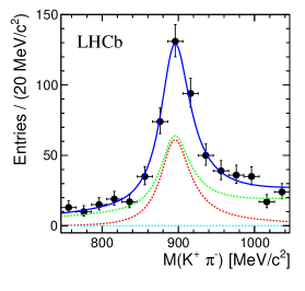
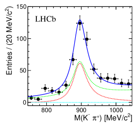
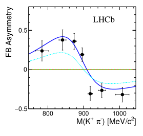
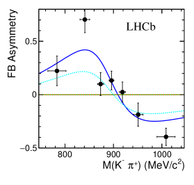
Figure 4: Projections of the model fitted to ${{B}^{0}_{s}}\rightarrow K^{+}\pi^{-}K^{-}\pi^{+}$ candidates (blue solid line) in the (top) invariant mass of $K\pi$ pairs and (bottom) $\cos\theta$ asymmetries as functions of $K\pi$ mass ($m_{1}$, $m_{2}$). The dots represent the data after background subtraction and acceptance correction. The red dashed line is the P–wave component, the green dashed line is the S–wave component and the light-blue dashed line represents the ${A}^{+}_{s}{A}_{0}$ interference term.

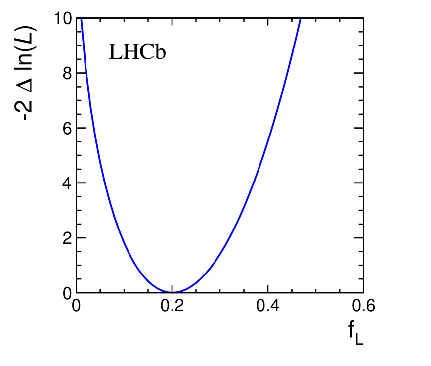
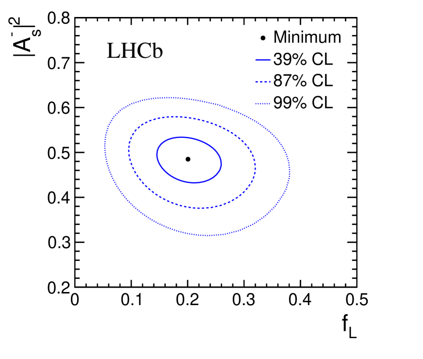
Figure 5: (Left) Profile likelihood for the parameter $f_{L}$. (Right) Regions corresponding to $\Delta\ln\mathcal{L}=$ 0.5, 2 and 4.5 (39%, 87% and 99% confidence level) in the $|A_{s}^{-}|^{2}$ – $f_{L}$ plane.

Table 5: Systematic uncertainties in the measurement of the magnitude and phase of the different amplitudes contributing to the ${{B}^{0}_{s}}\rightarrow K^{+}\pi^{-}K^{-}\pi^{+}$ decay.

Parameter	$\sigma_{\rm acc}$	$\sigma_{\rm sim}$	$\sigma_{\rm rw}$	$\sigma_{\rm mass}$	$\sigma_{\rm res}$	Total
$f_{L}$	0.031	0.010	0.010	0.021	0.006	0.040
$f_{\parallel}$	0.008	0.008	0.004	0.005	0.007	0.015
$|A_{s}^{+}|^{2}$	0.019	0.005	0.002	0.011	0.003	0.023
$|A_{s}^{-}|^{2}$	0.007	0.007	0.010	0.003	0.012	0.019
$|A_{ss}|^{2}$	0.003	0.001	0.000	0.005	0.003	0.007
$\delta_{\parallel}$	0.130	0.037	0.042	0.005	0.025	0.144
$\delta_{\perp}-\delta_{s}^{+}$	0.016	0.019	0.000	0.017	0.027	0.040
$\delta_{s}^{-}$	0.160	0.036	0.075	0.033	0.030	0.186
$\delta_{ss}$	0.096	0.076	0.188	0.018	0.044	0.229

The most important systematic uncertainties in the measurement of the different amplitudes, phases and polarisation fractions are summarised in Table 5. They arise mainly from uncertainties in the modelling of the $K\pi$ mass distributions and from the assumption that the five-dimensional acceptance factorises into a product of two-dimensional functions. To better exploit the statistical power of the simulated sample in the less populated regions of the phase space, e.g. the tails of the mass distribution, the angular and mass acceptances are assumed to factorise. An alternative model is tested that allows for correlation between the angular distribution and the $K\pi$ invariant mass, using a two-dimensional function in $(\cos\theta_{i},m_{i})$, universal for ${K}^{*0}$ and ${\kern 1.99997pt\overline{\kern-1.99997ptK}{}}{}^{*0}$ decays. The fit is repeated with this acceptance model and a systematic uncertainty, $\sigma_{\rm acc}$ , is determined from the variation with respect to the nominal fit result. An additional uncertainty accounts for the limited size of the simulated samples, $\sigma_{\rm sim}$.

To test the accuracy of the simulation, kinematic distributions, such as those of the $p_{\rm T}$ of final-state particles, are compared between data and simulation. Since the input amplitudes used in the generators are different from those measured in data, an iterative method is defined to disentangle the discrepancies associated with a different physical distribution. This procedure supports the quality of the simulation, and allows for the determination of the associated systematic uncertainty, $\sigma_{\rm rw}$.

Several alternative models for the parameterisation of invariant mass propagators are used and a systematic uncertainty, $\sigma_{\rm mass}$, for the fit parameters is estimated from the variation of the fit results. The main contribution to this uncertainty comes from the S–wave mass propagator, which is modelled by the LASS parameterisation [17] in the nominal fit. A combination of two spin-0 relativistic Breit-Wigner distributions with the mean and width of the $K^{*}_{0}(800)$ and $K^{*}_{0}(1430)$, respectively [19], and a single contribution from $K^{*}_{0}(1430)$ are also used.

Additional small uncertainties are considered to account for the effect of the invariant mass resolution, the lifetime acceptance and possible biases induced by the fitting method ($\sigma_{\rm res}$).

7 Measurement of ${{\cal B}({{B}^{0}_{s}}\rightarrow{{K}^{*0}}{{\kern 1.99997pt\overline{\kern-1.99997ptK}{}}{}^{*0}})}$

The branching fraction of the vector mode ${{B}^{0}_{s}}\rightarrow{{K}^{*0}}{{\kern 1.99997pt\overline{\kern-1.99997ptK}{}}{}^{*0}}$ is updated with respect to the previous result [8]. This measurement is normalised using the ${{B}^{0}}\rightarrow\phi{{K}^{*0}}$ decay, with $\phi\rightarrow K^{+}K^{-}$ and ${{K}^{*0}}\rightarrow K^{+}\pi^{-}$, which has a topology similar to the signal decay and a well-known branching fraction.

The selection of ${{B}^{0}}\rightarrow\phi{{K}^{*0}}$ decays is performed such that it closely resembles the selection of ${{B}^{0}_{s}}\rightarrow{{K}^{*0}}{{\kern 1.99997pt\overline{\kern-1.99997ptK}{}}{}^{*0}}$ decays, except for particle identification criteria. In particular, the requirements related to the ${B}^{0}_{s}$ vertex definition and the kinematic properties of the charged particles are identical. Figure 6 shows the invariant mass of the final-state particles for the selected candidates.

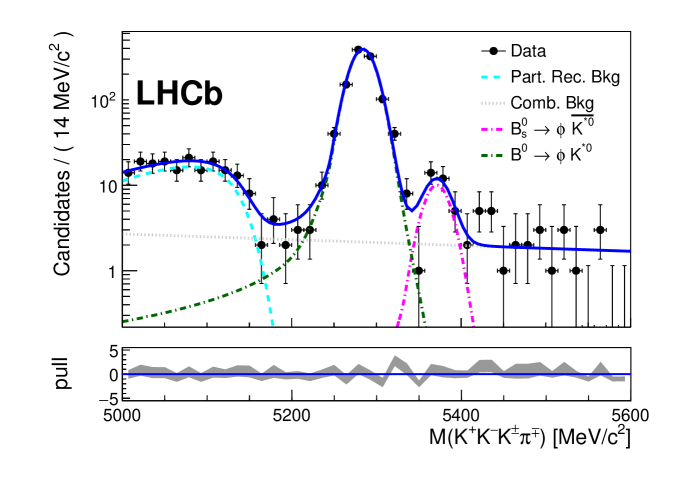
Figure 6: Invariant mass of the selected $K^{+}K^{-}K^{\pm}\pi^{\mp}$ combinations and result of the fit to the data. The points represent the data and the (blue) solid line is the fit model. The ${B}^{0}_{s}$ and ${B}^{0}$ signal peaks are shown as as dashed-dotted lines (pink and dark green, respectively). The contribution from partially reconstructed decays is represented as a (light blue) dashed line. The (grey) dotted line is the combinatorial background component. The normalised residual (pull) is shown below.

The ratio of branching fractions for signal and reference decay channels is given by

$$\frac{{\cal B}({{B}^{0}_{s}}\rightarrow{{K}^{*0}}{{\kern 1.99997pt\overline{\kern-1.99997ptK}{}}{}^{*0}})}{{\cal B}({{B}^{0}}\rightarrow\phi{{K}^{*0}})} = \frac{\varepsilon^{\rm sel}_{{{B}^{0}}\rightarrow\phi{{K}^{*0}}}}{\varepsilon^{\rm sel}_{{{B}^{0}_{s}}\rightarrow{{K}^{*0}}{{\kern 1.39998pt\overline{\kern-1.39998ptK}{}}{}^{*0}}}}\times\frac{\varepsilon^{\rm trig}_{{{B}^{0}}\rightarrow\phi{{K}^{*0}}}}{\varepsilon^{\rm trig}_{{{B}^{0}_{s}}\rightarrow{{K}^{*0}}{{\kern 1.39998pt\overline{\kern-1.39998ptK}{}}{}^{*0}}}}\times\frac{\lambda_{f_{L}}({{B}^{0}}\rightarrow\phi{{K}^{*0}})}{\lambda_{f_{L}}({{B}^{0}_{s}}\rightarrow{{K}^{*0}}{{\kern 1.99997pt\overline{\kern-1.99997ptK}{}}{}^{*0}})}$$ (35)

$$\times\frac{N_{{{B}^{0}_{s}}}\times f_{{{B}^{0}_{s}}\rightarrow{{K}^{*0}}{{\kern 1.39998pt\overline{\kern-1.39998ptK}{}}{}^{*0}}}}{N_{{{B}^{0}}}\times f_{{{B}^{0}}\rightarrow\phi{{K}^{*0}}}}\times\frac{f_{d}}{f_{s}}\times\frac{{\cal B}(\phi\rightarrow K^{+}K^{-})}{{\cal B}({{K}^{*0}}\rightarrow K^{+}\pi^{-})},$$

where $f_{d}/f_{s}$ is the ratio of probabilities for a $b$ quark to form a ${B}^{0}$ or a ${B}^{0}_{s}$ meson [35, 36].

The quantities $N_{{{B}^{0}_{s}}}$ and $N_{{{B}^{0}}}$ represent the number of observed candidates for ${{B}^{0}_{s}}\rightarrow K^{+}\pi^{-}K^{-}\pi^{+}$ and ${{B}^{0}}\rightarrow K^{+}K^{-}K^{\pm}\pi^{\mp}$ decays, respectively, and are determined from the corresponding fits to the four-body invariant mass spectra. The value of $N_{{{B}^{0}_{s}}}$ is reported in Sect. 4. The yield $N_{{{B}^{0}}}$ is extracted from an extended unbinned maximum likelihood fit to the spectrum in Fig. 6. The ${B}^{0}$ signal is modelled by a combination of Crystal Ball and Gaussian distributions that share a common mean. Their relative width, fraction and parameters describing the tail of the Crystal Ball function are set to the values determined from simulation. The signal from the recently observed decay ${{B}^{0}_{s}}\rightarrow\phi{{\kern 1.99997pt\overline{\kern-1.99997ptK}{}}{}^{*0}}$ [37] is also described using this parameterisation. The mass difference between ${B}^{0}$ and ${B}^{0}_{s}$ mesons is fixed to the world average value [19]. The partially reconstructed background is modelled using an ARGUS distribution with parameters free to vary in the fit. The combinatorial background is parameterised with a decreasing exponential function. A total of $1049\pm 33$ signal decays for the ${{B}^{0}}\rightarrow K^{+}K^{-}K^{\pm}\pi^{\mp}$ decay are observed.

The yield of candidates corresponding to the resonant decays, ${{B}^{0}_{s}}\rightarrow{{K}^{*0}}{{\kern 1.99997pt\overline{\kern-1.99997ptK}{}}{}^{*0}}$ and ${{B}^{0}}\rightarrow\phi{{K}^{*0}}$, is given by the purity factors $f_{{{B}^{0}_{s}}\rightarrow{{K}^{*0}}{{\kern 1.39998pt\overline{\kern-1.39998ptK}{}}{}^{*0}}}$ and $f_{{{B}^{0}}\rightarrow\phi{{K}^{*0}}}$. The ratio of combined reconstruction and selection efficiencies, $\varepsilon^{\rm sel}$, is calculated using ${{B}^{0}_{s}}\rightarrow{{K}^{*0}}{{\kern 1.99997pt\overline{\kern-1.99997ptK}{}}{}^{*0}}$ and ${{B}^{0}}\rightarrow\phi{{K}^{*0}}$ simulated events and validated using data. The inefficiency induced by the particle identification requirements is then determined separately using large calibration samples. The ratio of trigger efficiencies, $\varepsilon^{\rm trig}$, is computed through a data-driven method [38]. Moreover, the overall efficiency for each channel depends on the helicity angle distribution of the final state particles, and is encoded into the factors $\lambda_{f_{L}}$. Both the purity and $\lambda_{f_{L}}$ factors for the ${{B}^{0}_{s}}\rightarrow{{K}^{*0}}{{\kern 1.99997pt\overline{\kern-1.99997ptK}{}}{}^{*0}}$ decay are calculated from the results of the angular analysis. Those corresponding to ${{B}^{0}}\rightarrow\phi{{K}^{*0}}$ decays are calculated from Ref. [39].

Table 6: Summary of relevant quantities in the ${\cal B}({{B}^{0}_{s}}\rightarrow{{K}^{*0}}{{\kern 1.99997pt\overline{\kern-1.99997ptK}{}}{}^{*0}})$ calculation. The factor $\kappa({{B}^{0}_{s}}\rightarrow{{K}^{*0}}{{\kern 1.99997pt\overline{\kern-1.99997ptK}{}}{}^{*0}})$ is defined as $\lambda_{f_{L}}({{B}^{0}_{s}}\rightarrow{{K}^{*0}}{{\kern 1.99997pt\overline{\kern-1.99997ptK}{}}{}^{*0}})/f_{{{B}^{0}_{s}}\rightarrow{{K}^{*0}}{{\kern 1.39998pt\overline{\kern-1.39998ptK}{}}{}^{*0}}}$, and equivalently for the ${{B}^{0}}\rightarrow\phi{{K}^{*0}}$ decay. The first uncertainty is statistical, the second systematic.

$N_{{{B}^{0}_{s}}}$	$697\pm 31\pm 11$
$N_{{{B}^{0}}}$	$1049\pm 33\pm\phantom{0}7$
$\kappa_{{{B}^{0}}\rightarrow\phi{{K}^{*0}}}/\kappa_{{{B}^{0}_{s}}\rightarrow{{K}^{*0}}{{\kern 1.39998pt\overline{\kern-1.39998ptK}{}}{}^{*0}}}$	$0.453\pm 0.059\pm 0.040$
$\varepsilon_{{{B}^{0}}\rightarrow\phi{{K}^{*0}}}/\varepsilon_{{{B}^{0}_{s}}\rightarrow{{K}^{*0}}{{\kern 1.39998pt\overline{\kern-1.39998ptK}{}}{}^{*0}}}$	$1.30\phantom{0}\pm 0.17\phantom{0}\pm 0.07\phantom{0}$

With the factors summarised in Table 6, the ratio of branching fractions is determined to be

$$\frac{{\cal B}({{B}^{0}_{s}}\rightarrow{{K}^{*0}}{{\kern 1.99997pt\overline{\kern-1.99997ptK}{}}{}^{*0}})}{{\cal B}({{B}^{0}}\rightarrow\phi{{K}^{*0}})}=1.11\pm 0.22({\rm stat.})\pm 0.12({\rm syst.})\pm 0.06(f_{d}/f_{s}).$$ (36)

Using the average ${\cal B}({{B}^{0}}\rightarrow\phi{{K}^{*0}})=(9.73\pm 0.72)\times 10^{-6}$ from the BaBar [18] and Belle [40] measurements, corrected to take into account different rates of $B^{+}B^{-}$ and $B^{0}\bar{B}^{0}$ pair production from $\Upsilon(4S)$ using ${\Gamma(B^{+}B^{-})}/{\Gamma(B^{0}\bar{B}^{0})}=1.055\pm 0.025$ [19], the result obtained is

$${\cal B}({{B}^{0}_{s}}\rightarrow{{K}^{*0}}{{\kern 1.99997pt\overline{\kern-1.99997ptK}{}}{}^{*0}})=(10.8\pm 2.1\,{\rm(stat.)}\pm 1.4\,{\rm(syst.)}\pm 0.6\,(f_{d}/f_{s}))\times 10^{-6}.$$

The main systematic uncertainties considered are related to the invariant mass fit used to determine the signal and reference event yields, the angular correction, and the determination of the trigger efficiency. To determine the systematic uncertainty associated with the number of candidates, the fit is repeated using different models for the signal and background components. The largest variation is assigned as a 1.7% systematic uncertainty. A 5% uncertainty is attributed to the trigger efficiency, after calibration of the data-driven method applied to both channels using fully simulated events. The systematic uncertainty associated with the angular correction $\lambda_{f_{L}}$ is the result of the propagation of the systematic uncertainties evaluated for the parameters measured in the angular analysis (9%).

This result supersedes the previous measurement [8], which used a less sophisticated estimate of the S–wave contribution. If rescaled to the same S–wave fraction, both results are compatible.

As a result of ${{B}^{0}_{s}}$–${{\kern 1.79993pt\overline{\kern-1.79993ptB}{}}{}^{0}_{s}}$ mixing, the time-integrated flavour-averaged branching fraction (${\cal B}$) reported here cannot be directly compared with theoretical predictions formulated in terms of the decay amplitudes at $t=0$ (${\cal B}_{0}$). The relation between these branching fractions is given by [33]

$${\cal B}\;=\;f_{\Delta\Gamma}\;{\cal B}_{0},\quad\text{with}\quad f_{\Delta\Gamma}\;=\;\left(1-\frac{\Delta\Gamma_{s}}{2\Gamma_{s}}\left(f_{L}+f_{\parallel}+f_{\perp}\right)\right)\;.$$ (37)

Using the decay widths measured in Ref. [34] and the polarisation fractions reported here, the correction factor is calculated to be $f_{\Delta\Gamma}=1.015\pm 0.010$.

8 Conclusions

The decay ${{B}^{0}_{s}}\rightarrow K^{+}\pi^{-}K^{-}\pi^{+}$ is studied using $pp$ collision data recorded by LHCb during 2011 at a centre-of-mass energy $\sqrt{s}=7$$\mathrm{\,Te\kern-1.00006ptV}$. This sample corresponds to an integrated luminosity of 1.0$\mbox{\,fb}^{-1}$.

A test of the SM is performed by measuring eight $C\!P$-violating quantities which are predicted to be small in the SM. All of these are found to be compatible with the SM expectation, within $2\sigma$ uncertainty. In addition, assuming no $C\!P$ violation, the angular distribution of the decay products is analysed as a function of the $K\pi$ pair invariant mass to measure the polarisation fractions of the decay ${{B}^{0}_{s}}\rightarrow{{K}^{*0}}{{\kern 1.99997pt\overline{\kern-1.99997ptK}{}}{}^{*0}}$ as well as the magnitude and phase of the various S–wave amplitudes. The low polarisation of the vector-vector decay is confirmed by the measurement $f_{L}=0.201\pm 0.057\,{\rm(stat.)}\pm 0.040\,{\rm(syst.)}$, and a large S–wave contribution is found.

Finally, an update of the ${{B}^{0}_{s}}\rightarrow{{K}^{*0}}{{\kern 1.99997pt\overline{\kern-1.99997ptK}{}}{}^{*0}}$ branching fraction, using the ${{B}^{0}}\rightarrow\phi{{K}^{*0}}$ decay as normalisation channel, yields ${\cal B}({{B}^{0}_{s}}\rightarrow{{K}^{*0}}{{\kern 1.99997pt\overline{\kern-1.99997ptK}{}}{}^{*0}})=(10.8\pm 2.1\,{\rm(stat.)}\pm 1.4\,{\rm(syst.)}\pm 0.6\,(f_{d}/f_{s}))\times 10^{-6}$, in agreement with the theoretical prediction [7]. This result takes into account the S–wave component measured for the first time through the angular analysis of ${{B}^{0}_{s}}\rightarrow K^{+}\pi^{-}K^{-}\pi^{+}$ decays and supersedes the measurement in Ref. [8].

LHCb collaboration

R. Aaij⁴¹, B. Adeva³⁷, M. Adinolfi⁴⁶, A. Affolder⁵², Z. Ajaltouni⁵, S. Akar⁶, J. Albrecht⁹, F. Alessio³⁸, M. Alexander⁵¹, S. Ali⁴¹, G. Alkhazov³⁰, P. Alvarez Cartelle⁵³, A.A. Alves Jr^25,38, S. Amato², S. Amerio²², Y. Amhis⁷, L. An³, L. Anderlini^17,g, J. Anderson⁴⁰, R. Andreassen⁵⁷, M. Andreotti^16,f, J.E. Andrews⁵⁸, R.B. Appleby⁵⁴, O. Aquines Gutierrez¹⁰, F. Archilli³⁸, A. Artamonov³⁵, M. Artuso⁵⁹, E. Aslanides⁶, G. Auriemma^25,n, M. Baalouch⁵, S. Bachmann¹¹, J.J. Back⁴⁸, A. Badalov³⁶, C. Baesso⁶⁰, W. Baldini¹⁶, R.J. Barlow⁵⁴, C. Barschel³⁸, S. Barsuk⁷, W. Barter³⁸, V. Batozskaya²⁸, V. Battista³⁹, A. Bay³⁹, L. Beaucourt⁴, J. Beddow⁵¹, F. Bedeschi²³, I. Bediaga¹, L.J. Bel⁴¹, S. Belogurov³¹, I. Belyaev³¹, E. Ben-Haim⁸, G. Bencivenni¹⁸, S. Benson³⁸, J. Benton⁴⁶, A. Berezhnoy³², R. Bernet⁴⁰, A. Bertolin²², M.-O. Bettler⁴⁷, M. van Beuzekom⁴¹, A. Bien¹¹, S. Bifani⁴⁵, T. Bird⁵⁴, A. Bizzeti^17,i, T. Blake⁴⁸, F. Blanc³⁹, J. Blouw¹⁰, S. Blusk⁵⁹, V. Bocci²⁵, A. Bondar³⁴, N. Bondar^30,38, W. Bonivento¹⁵, S. Borghi⁵⁴, A. Borgia⁵⁹, M. Borsato⁷, T.J.V. Bowcock⁵², E. Bowen⁴⁰, C. Bozzi¹⁶, D. Brett⁵⁴, M. Britsch¹⁰, T. Britton⁵⁹, J. Brodzicka⁵⁴, N.H. Brook⁴⁶, A. Bursche⁴⁰, J. Buytaert³⁸, S. Cadeddu¹⁵, R. Calabrese^16,f, M. Calvi^20,k, M. Calvo Gomez^36,p, P. Campana¹⁸, D. Campora Perez³⁸, L. Capriotti⁵⁴, A. Carbone^14,d, G. Carboni^24,l, R. Cardinale^19,38,j, A. Cardini¹⁵, P. Carniti²⁰, L. Carson⁵⁰, K. Carvalho Akiba^2,38, R. Casanova Mohr³⁶, G. Casse⁵², L. Cassina^20,k, L. Castillo Garcia³⁸, M. Cattaneo³⁸, Ch. Cauet⁹, G. Cavallero¹⁹, R. Cenci^23,t, M. Charles⁸, Ph. Charpentier³⁸, M. Chefdeville⁴, S. Chen⁵⁴, S.-F. Cheung⁵⁵, N. Chiapolini⁴⁰, M. Chrzaszcz^40,26, X. Cid Vidal³⁸, G. Ciezarek⁴¹, P.E.L. Clarke⁵⁰, M. Clemencic³⁸, H.V. Cliff⁴⁷, J. Closier³⁸, V. Coco³⁸, J. Cogan⁶, E. Cogneras⁵, V. Cogoni^15,e, L. Cojocariu²⁹, G. Collazuol²², P. Collins³⁸, A. Comerma-Montells¹¹, A. Contu^15,38, A. Cook⁴⁶, M. Coombes⁴⁶, S. Coquereau⁸, G. Corti³⁸, M. Corvo^16,f, I. Counts⁵⁶, B. Couturier³⁸, G.A. Cowan⁵⁰, D.C. Craik⁴⁸, A.C. Crocombe⁴⁸, M. Cruz Torres⁶⁰, S. Cunliffe⁵³, R. Currie⁵³, C. D’Ambrosio³⁸, J. Dalseno⁴⁶, P. David⁸, P.N.Y. David⁴¹, A. Davis⁵⁷, K. De Bruyn⁴¹, S. De Capua⁵⁴, M. De Cian¹¹, J.M. De Miranda¹, L. De Paula², W. De Silva⁵⁷, P. De Simone¹⁸, C.-T. Dean⁵¹, D. Decamp⁴, M. Deckenhoff⁹, L. Del Buono⁸, N. Déléage⁴, D. Derkach⁵⁵, O. Deschamps⁵, F. Dettori³⁸, B. Dey⁴⁰, A. Di Canto³⁸, F. Di Ruscio²⁴, H. Dijkstra³⁸, S. Donleavy⁵², F. Dordei¹¹, M. Dorigo³⁹, A. Dosil Suárez³⁷, D. Dossett⁴⁸, A. Dovbnya⁴³, K. Dreimanis⁵², G. Dujany⁵⁴, F. Dupertuis³⁹, P. Durante⁶, R. Dzhelyadin³⁵, A. Dziurda²⁶, A. Dzyuba³⁰, S. Easo^49,38, U. Egede⁵³, V. Egorychev³¹, S. Eidelman³⁴, S. Eisenhardt⁵⁰, U. Eitschberger⁹, R. Ekelhof⁹, L. Eklund⁵¹, I. El Rifai⁵, Ch. Elsasser⁴⁰, S. Ely⁵⁹, S. Esen¹¹, H.M. Evans⁴⁷, T. Evans⁵⁵, A. Falabella¹⁴, C. Färber¹¹, C. Farinelli⁴¹, N. Farley⁴⁵, S. Farry⁵², R. Fay⁵², D. Ferguson⁵⁰, V. Fernandez Albor³⁷, F. Ferreira Rodrigues¹, M. Ferro-Luzzi³⁸, S. Filippov³³, M. Fiore^16,f, M. Fiorini^16,f, M. Firlej²⁷, C. Fitzpatrick³⁹, T. Fiutowski²⁷, P. Fol⁵³, M. Fontana¹⁰, F. Fontanelli^19,j, R. Forty³⁸, O. Francisco², M. Frank³⁸, C. Frei³⁸, M. Frosini¹⁷, J. Fu^21,38, E. Furfaro^24,l, A. Gallas Torreira³⁷, D. Galli^14,d, S. Gallorini^22,38, S. Gambetta^19,j, M. Gandelman², P. Gandini⁵⁹, Y. Gao³, J. García Pardiñas³⁷, J. Garofoli⁵⁹, J. Garra Tico⁴⁷, L. Garrido³⁶, D. Gascon³⁶, C. Gaspar³⁸, U. Gastaldi¹⁶, R. Gauld⁵⁵, L. Gavardi⁹, G. Gazzoni⁵, A. Geraci^21,v, E. Gersabeck¹¹, M. Gersabeck⁵⁴, T. Gershon⁴⁸, Ph. Ghez⁴, A. Gianelle²², S. Gianì³⁹, V. Gibson⁴⁷, L. Giubega²⁹, V.V. Gligorov³⁸, C. Göbel⁶⁰, D. Golubkov³¹, A. Golutvin^53,31,38, A. Gomes^1,a, C. Gotti^20,k, M. Grabalosa Gándara⁵, R. Graciani Diaz³⁶, L.A. Granado Cardoso³⁸, E. Graugés³⁶, E. Graverini⁴⁰, G. Graziani¹⁷, A. Grecu²⁹, E. Greening⁵⁵, S. Gregson⁴⁷, P. Griffith⁴⁵, L. Grillo¹¹, O. Grünberg⁶³, B. Gui⁵⁹, E. Gushchin³³, Yu. Guz^35,38, T. Gys³⁸, C. Hadjivasiliou⁵⁹, G. Haefeli³⁹, C. Haen³⁸, S.C. Haines⁴⁷, S. Hall⁵³, B. Hamilton⁵⁸, T. Hampson⁴⁶, X. Han¹¹, S. Hansmann-Menzemer¹¹, N. Harnew⁵⁵, S.T. Harnew⁴⁶, J. Harrison⁵⁴, J. He³⁸, T. Head³⁹, V. Heijne⁴¹, K. Hennessy⁵², P. Henrard⁵, L. Henry⁸, J.A. Hernando Morata³⁷, E. van Herwijnen³⁸, M. Heß⁶³, A. Hicheur², D. Hill⁵⁵, M. Hoballah⁵, C. Hombach⁵⁴, W. Hulsbergen⁴¹, T. Humair⁵³, N. Hussain⁵⁵, D. Hutchcroft⁵², D. Hynds⁵¹, M. Idzik²⁷, P. Ilten⁵⁶, R. Jacobsson³⁸, A. Jaeger¹¹, J. Jalocha⁵⁵, E. Jans⁴¹, A. Jawahery⁵⁸, F. Jing³, M. John⁵⁵, D. Johnson³⁸, C.R. Jones⁴⁷, C. Joram³⁸, B. Jost³⁸, N. Jurik⁵⁹, S. Kandybei⁴³, W. Kanso⁶, M. Karacson³⁸, T.M. Karbach³⁸, S. Karodia⁵¹, M. Kelsey⁵⁹, I.R. Kenyon⁴⁵, M. Kenzie³⁸, T. Ketel⁴², B. Khanji^20,38,k, C. Khurewathanakul³⁹, S. Klaver⁵⁴, K. Klimaszewski²⁸, O. Kochebina⁷, M. Kolpin¹¹, I. Komarov³⁹, R.F. Koopman⁴², P. Koppenburg^41,38, M. Korolev³², L. Kravchuk³³, K. Kreplin¹¹, M. Kreps⁴⁸, G. Krocker¹¹, P. Krokovny³⁴, F. Kruse⁹, W. Kucewicz^26,o, M. Kucharczyk^20,k, V. Kudryavtsev³⁴, K. Kurek²⁸, T. Kvaratskheliya³¹, V.N. La Thi³⁹, D. Lacarrere³⁸, G. Lafferty⁵⁴, A. Lai¹⁵, D. Lambert⁵⁰, R.W. Lambert⁴², G. Lanfranchi¹⁸, C. Langenbruch⁴⁸, B. Langhans³⁸, T. Latham⁴⁸, C. Lazzeroni⁴⁵, R. Le Gac⁶, J. van Leerdam⁴¹, J.-P. Lees⁴, R. Lefèvre⁵, A. Leflat³², J. Lefrançois⁷, O. Leroy⁶, T. Lesiak²⁶, B. Leverington¹¹, Y. Li⁷, T. Likhomanenko⁶⁴, M. Liles⁵², R. Lindner³⁸, C. Linn³⁸, F. Lionetto⁴⁰, B. Liu¹⁵, S. Lohn³⁸, I. Longstaff⁵¹, J.H. Lopes², P. Lowdon⁴⁰, D. Lucchesi^22,r, H. Luo⁵⁰, A. Lupato²², E. Luppi^16,f, O. Lupton⁵⁵, F. Machefert⁷, I.V. Machikhiliyan³¹, F. Maciuc²⁹, O. Maev³⁰, S. Malde⁵⁵, A. Malinin⁶⁴, G. Manca^15,e, G. Mancinelli⁶, P. Manning⁵⁹, A. Mapelli³⁸, J. Maratas⁵, J.F. Marchand⁴, U. Marconi¹⁴, C. Marin Benito³⁶, P. Marino^23,t, R. Märki³⁹, J. Marks¹¹, G. Martellotti²⁵, M. Martinelli³⁹, D. Martinez Santos⁴², F. Martinez Vidal⁶⁶, D. Martins Tostes², A. Massafferri¹, R. Matev³⁸, Z. Mathe³⁸, C. Matteuzzi²⁰, A. Mauri⁴⁰, B. Maurin³⁹, A. Mazurov⁴⁵, M. McCann⁵³, J. McCarthy⁴⁵, A. McNab⁵⁴, R. McNulty¹², B. McSkelly⁵², B. Meadows⁵⁷, F. Meier⁹, M. Meissner¹¹, M. Merk⁴¹, D.A. Milanes⁶², M.-N. Minard⁴, J. Molina Rodriguez⁶⁰, S. Monteil⁵, M. Morandin²², P. Morawski²⁷, A. Mordà⁶, M.J. Morello^23,t, J. Moron²⁷, A.-B. Morris⁵⁰, R. Mountain⁵⁹, F. Muheim⁵⁰, K. Müller⁴⁰, M. Mussini¹⁴, B. Muster³⁹, P. Naik⁴⁶, T. Nakada³⁹, R. Nandakumar⁴⁹, I. Nasteva², M. Needham⁵⁰, N. Neri²¹, S. Neubert¹¹, N. Neufeld³⁸, M. Neuner¹¹, A.D. Nguyen³⁹, T.D. Nguyen³⁹, C. Nguyen-Mau^39,q, M. Nicol⁷, V. Niess⁵, R. Niet⁹, N. Nikitin³², T. Nikodem¹¹, A. Novoselov³⁵, D.P. O’Hanlon⁴⁸, A. Oblakowska-Mucha²⁷, V. Obraztsov³⁵, S. Ogilvy⁵¹, O. Okhrimenko⁴⁴, R. Oldeman^15,e, C.J.G. Onderwater⁶⁷, B. Osorio Rodrigues¹, J.M. Otalora Goicochea², A. Otto³⁸, P. Owen⁵³, A. Oyanguren⁶⁶, B.K. Pal⁵⁹, A. Palano^13,c, F. Palombo^21,u, M. Palutan¹⁸, J. Panman³⁸, A. Papanestis⁴⁹, M. Pappagallo⁵¹, L.L. Pappalardo^16,f, C. Parkes⁵⁴, C.J. Parkinson^9,45, G. Passaleva¹⁷, G.D. Patel⁵², M. Patel⁵³, C. Patrignani^19,j, A. Pearce^54,49, A. Pellegrino⁴¹, G. Penso^25,m, M. Pepe Altarelli³⁸, S. Perazzini^14,d, P. Perret⁵, L. Pescatore⁴⁵, K. Petridis⁴⁶, A. Petrolini^19,j, E. Picatoste Olloqui³⁶, B. Pietrzyk⁴, T. Pilař⁴⁸, D. Pinci²⁵, A. Pistone¹⁹, S. Playfer⁵⁰, M. Plo Casasus³⁷, F. Polci⁸, A. Poluektov^48,34, I. Polyakov³¹, E. Polycarpo², A. Popov³⁵, D. Popov¹⁰, B. Popovici²⁹, C. Potterat², E. Price⁴⁶, J.D. Price⁵², J. Prisciandaro³⁹, A. Pritchard⁵², C. Prouve⁴⁶, V. Pugatch⁴⁴, A. Puig Navarro³⁹, G. Punzi^23,s, W. Qian⁴, R. Quagliani^7,46, B. Rachwal²⁶, J.H. Rademacker⁴⁶, B. Rakotomiaramanana³⁹, M. Rama²³, M.S. Rangel², I. Raniuk⁴³, N. Rauschmayr³⁸, G. Raven⁴², F. Redi⁵³, S. Reichert⁵⁴, M.M. Reid⁴⁸, A.C. dos Reis¹, S. Ricciardi⁴⁹, S. Richards⁴⁶, M. Rihl³⁸, K. Rinnert⁵², V. Rives Molina³⁶, P. Robbe⁷, A.B. Rodrigues¹, E. Rodrigues⁵⁴, P. Rodriguez Perez⁵⁴, S. Roiser³⁸, V. Romanovsky³⁵, A. Romero Vidal³⁷, M. Rotondo²², J. Rouvinet³⁹, T. Ruf³⁸, H. Ruiz³⁶, P. Ruiz Valls⁶⁶, J.J. Saborido Silva³⁷, N. Sagidova³⁰, P. Sail⁵¹, B. Saitta^15,e, V. Salustino Guimaraes², C. Sanchez Mayordomo⁶⁶, B. Sanmartin Sedes³⁷, R. Santacesaria²⁵, C. Santamarina Rios³⁷, E. Santovetti^24,l, A. Sarti^18,m, C. Satriano^25,n, A. Satta²⁴, D.M. Saunders⁴⁶, D. Savrina^31,32, M. Schiller³⁸, H. Schindler³⁸, M. Schlupp⁹, M. Schmelling¹⁰, B. Schmidt³⁸, O. Schneider³⁹, A. Schopper³⁸, M.-H. Schune⁷, R. Schwemmer³⁸, B. Sciascia¹⁸, A. Sciubba^25,m, A. Semennikov³¹, I. Sepp⁵³, N. Serra⁴⁰, J. Serrano⁶, L. Sestini²², P. Seyfert¹¹, M. Shapkin³⁵, I. Shapoval^16,43,f, Y. Shcheglov³⁰, T. Shears⁵², L. Shekhtman³⁴, V. Shevchenko⁶⁴, A. Shires⁹, R. Silva Coutinho⁴⁸, G. Simi²², M. Sirendi⁴⁷, N. Skidmore⁴⁶, I. Skillicorn⁵¹, T. Skwarnicki⁵⁹, N.A. Smith⁵², E. Smith^55,49, E. Smith⁵³, J. Smith⁴⁷, M. Smith⁵⁴, H. Snoek⁴¹, M.D. Sokoloff⁵⁷, F.J.P. Soler⁵¹, F. Soomro³⁹, D. Souza⁴⁶, B. Souza De Paula², B. Spaan⁹, P. Spradlin⁵¹, S. Sridharan³⁸, F. Stagni³⁸, M. Stahl¹¹, S. Stahl³⁸, O. Steinkamp⁴⁰, O. Stenyakin³⁵, F. Sterpka⁵⁹, S. Stevenson⁵⁵, S. Stoica²⁹, S. Stone⁵⁹, B. Storaci⁴⁰, S. Stracka^23,t, M. Straticiuc²⁹, U. Straumann⁴⁰, R. Stroili²², L. Sun⁵⁷, W. Sutcliffe⁵³, K. Swientek²⁷, S. Swientek⁹, V. Syropoulos⁴², M. Szczekowski²⁸, P. Szczypka^39,38, T. Szumlak²⁷, S. T’Jampens⁴, M. Teklishyn⁷, G. Tellarini^16,f, F. Teubert³⁸, C. Thomas⁵⁵, E. Thomas³⁸, J. van Tilburg⁴¹, V. Tisserand⁴, M. Tobin³⁹, J. Todd⁵⁷, S. Tolk⁴², L. Tomassetti^16,f, D. Tonelli³⁸, S. Topp-Joergensen⁵⁵, N. Torr⁵⁵, E. Tournefier⁴, S. Tourneur³⁹, K. Trabelsi³⁹, M.T. Tran³⁹, M. Tresch⁴⁰, A. Trisovic³⁸, A. Tsaregorodtsev⁶, P. Tsopelas⁴¹, N. Tuning^41,38, M. Ubeda Garcia³⁸, A. Ukleja²⁸, A. Ustyuzhanin⁶⁵, U. Uwer¹¹, C. Vacca^15,e, V. Vagnoni¹⁴, G. Valenti¹⁴, A. Vallier⁷, R. Vazquez Gomez¹⁸, P. Vazquez Regueiro³⁷, C. Vázquez Sierra³⁷, S. Vecchi¹⁶, J.J. Velthuis⁴⁶, M. Veltri^17,h, G. Veneziano³⁹, M. Vesterinen¹¹, J.V. Viana Barbosa³⁸, B. Viaud⁷, D. Vieira², M. Vieites Diaz³⁷, X. Vilasis-Cardona^36,p, A. Vollhardt⁴⁰, D. Volyanskyy¹⁰, D. Voong⁴⁶, A. Vorobyev³⁰, V. Vorobyev³⁴, C. Voß⁶³, J.A. de Vries⁴¹, R. Waldi⁶³, C. Wallace⁴⁸, R. Wallace¹², J. Walsh²³, S. Wandernoth¹¹, J. Wang⁵⁹, D.R. Ward⁴⁷, N.K. Watson⁴⁵, D. Websdale⁵³, M. Whitehead⁴⁸, D. Wiedner¹¹, G. Wilkinson^55,38, M. Wilkinson⁵⁹, M.P. Williams⁴⁵, M. Williams⁵⁶, H.W. Wilschut⁶⁷, F.F. Wilson⁴⁹, J. Wimberley⁵⁸, J. Wishahi⁹, W. Wislicki²⁸, M. Witek²⁶, G. Wormser⁷, S.A. Wotton⁴⁷, S. Wright⁴⁷, K. Wyllie³⁸, Y. Xie⁶¹, Z. Xing⁵⁹, Z. Xu³⁹, Z. Yang³, X. Yuan³⁴, O. Yushchenko³⁵, M. Zangoli¹⁴, M. Zavertyaev^10,b, L. Zhang³, W.C. Zhang¹², Y. Zhang³, A. Zhelezov¹¹, A. Zhokhov³¹, L. Zhong³.

¹Centro Brasileiro de Pesquisas Físicas (CBPF), Rio de Janeiro, Brazil
²Universidade Federal do Rio de Janeiro (UFRJ), Rio de Janeiro, Brazil
³Center for High Energy Physics, Tsinghua University, Beijing, China
⁴LAPP, Université Savoie Mont-Blanc, CNRS/IN2P3, Annecy-Le-Vieux, France
⁵Clermont Université, Université Blaise Pascal, CNRS/IN2P3, LPC, Clermont-Ferrand, France
⁶CPPM, Aix-Marseille Université, CNRS/IN2P3, Marseille, France
⁷LAL, Université Paris-Sud, CNRS/IN2P3, Orsay, France
⁸LPNHE, Université Pierre et Marie Curie, Université Paris Diderot, CNRS/IN2P3, Paris, France
⁹Fakultät Physik, Technische Universität Dortmund, Dortmund, Germany
¹⁰Max-Planck-Institut für Kernphysik (MPIK), Heidelberg, Germany
¹¹Physikalisches Institut, Ruprecht-Karls-Universität Heidelberg, Heidelberg, Germany
¹²School of Physics, University College Dublin, Dublin, Ireland
¹³Sezione INFN di Bari, Bari, Italy
¹⁴Sezione INFN di Bologna, Bologna, Italy
¹⁵Sezione INFN di Cagliari, Cagliari, Italy
¹⁶Sezione INFN di Ferrara, Ferrara, Italy
¹⁷Sezione INFN di Firenze, Firenze, Italy
¹⁸Laboratori Nazionali dell’INFN di Frascati, Frascati, Italy
¹⁹Sezione INFN di Genova, Genova, Italy
²⁰Sezione INFN di Milano Bicocca, Milano, Italy
²¹Sezione INFN di Milano, Milano, Italy
²²Sezione INFN di Padova, Padova, Italy
²³Sezione INFN di Pisa, Pisa, Italy
²⁴Sezione INFN di Roma Tor Vergata, Roma, Italy
²⁵Sezione INFN di Roma La Sapienza, Roma, Italy
²⁶Henryk Niewodniczanski Institute of Nuclear Physics Polish Academy of Sciences, Kraków, Poland
²⁷AGH - University of Science and Technology, Faculty of Physics and Applied Computer Science, Kraków, Poland
²⁸National Center for Nuclear Research (NCBJ), Warsaw, Poland
²⁹Horia Hulubei National Institute of Physics and Nuclear Engineering, Bucharest-Magurele, Romania
³⁰Petersburg Nuclear Physics Institute (PNPI), Gatchina, Russia
³¹Institute of Theoretical and Experimental Physics (ITEP), Moscow, Russia
³²Institute of Nuclear Physics, Moscow State University (SINP MSU), Moscow, Russia
³³Institute for Nuclear Research of the Russian Academy of Sciences (INR RAN), Moscow, Russia
³⁴Budker Institute of Nuclear Physics (SB RAS) and Novosibirsk State University, Novosibirsk, Russia
³⁵Institute for High Energy Physics (IHEP), Protvino, Russia
³⁶Universitat de Barcelona, Barcelona, Spain
³⁷Universidad de Santiago de Compostela, Santiago de Compostela, Spain
³⁸European Organization for Nuclear Research (CERN), Geneva, Switzerland
³⁹Ecole Polytechnique Fédérale de Lausanne (EPFL), Lausanne, Switzerland
⁴⁰Physik-Institut, Universität Zürich, Zürich, Switzerland
⁴¹Nikhef National Institute for Subatomic Physics, Amsterdam, The Netherlands
⁴²Nikhef National Institute for Subatomic Physics and VU University Amsterdam, Amsterdam, The Netherlands
⁴³NSC Kharkiv Institute of Physics and Technology (NSC KIPT), Kharkiv, Ukraine
⁴⁴Institute for Nuclear Research of the National Academy of Sciences (KINR), Kyiv, Ukraine
⁴⁵University of Birmingham, Birmingham, United Kingdom
⁴⁶H.H. Wills Physics Laboratory, University of Bristol, Bristol, United Kingdom
⁴⁷Cavendish Laboratory, University of Cambridge, Cambridge, United Kingdom
⁴⁸Department of Physics, University of Warwick, Coventry, United Kingdom
⁴⁹STFC Rutherford Appleton Laboratory, Didcot, United Kingdom
⁵⁰School of Physics and Astronomy, University of Edinburgh, Edinburgh, United Kingdom
⁵¹School of Physics and Astronomy, University of Glasgow, Glasgow, United Kingdom
⁵²Oliver Lodge Laboratory, University of Liverpool, Liverpool, United Kingdom
⁵³Imperial College London, London, United Kingdom
⁵⁴School of Physics and Astronomy, University of Manchester, Manchester, United Kingdom
⁵⁵Department of Physics, University of Oxford, Oxford, United Kingdom
⁵⁶Massachusetts Institute of Technology, Cambridge, MA, United States
⁵⁷University of Cincinnati, Cincinnati, OH, United States
⁵⁸University of Maryland, College Park, MD, United States
⁵⁹Syracuse University, Syracuse, NY, United States
⁶⁰Pontifícia Universidade Católica do Rio de Janeiro (PUC-Rio), Rio de Janeiro, Brazil, associated to ^2
61Institute of Particle Physics, Central China Normal University, Wuhan, Hubei, China, associated to ^3
62Departamento de Fisica , Universidad Nacional de Colombia, Bogota, Colombia, associated to ^8
63Institut für Physik, Universität Rostock, Rostock, Germany, associated to ^11
64National Research Centre Kurchatov Institute, Moscow, Russia, associated to ^31
65Yandex School of Data Analysis, Moscow, Russia, associated to ^31
66Instituto de Fisica Corpuscular (IFIC), Universitat de Valencia-CSIC, Valencia, Spain, associated to ^36
67Van Swinderen Institute, University of Groningen, Groningen, The Netherlands, associated to <sup>41

a</sup>Universidade Federal do Triângulo Mineiro (UFTM), Uberaba-MG, Brazil
^bP.N. Lebedev Physical Institute, Russian Academy of Science (LPI RAS), Moscow, Russia
^cUniversità di Bari, Bari, Italy
^dUniversità di Bologna, Bologna, Italy
^eUniversità di Cagliari, Cagliari, Italy
^fUniversità di Ferrara, Ferrara, Italy
^gUniversità di Firenze, Firenze, Italy
^hUniversità di Urbino, Urbino, Italy
ⁱUniversità di Modena e Reggio Emilia, Modena, Italy
^jUniversità di Genova, Genova, Italy
^kUniversità di Milano Bicocca, Milano, Italy
^lUniversità di Roma Tor Vergata, Roma, Italy
^mUniversità di Roma La Sapienza, Roma, Italy
ⁿUniversità della Basilicata, Potenza, Italy
^oAGH - University of Science and Technology, Faculty of Computer Science, Electronics and Telecommunications, Kraków, Poland
^pLIFAELS, La Salle, Universitat Ramon Llull, Barcelona, Spain
^qHanoi University of Science, Hanoi, Viet Nam
^rUniversità di Padova, Padova, Italy
^sUniversità di Pisa, Pisa, Italy
^tScuola Normale Superiore, Pisa, Italy
^uUniversità degli Studi di Milano, Milano, Italy
^vPolitecnico di Milano, Milano, Italy

References

- [1] R. Fleischer, Extracting CKM phases from angular distributions of decays into admixtures of CP eigenstates, Phys. Rev. D60 (1999) 073008, arXiv:hep-ph/9903540
- [2] M. Ciuchini, M. Pierini, and L. Silvestrini, decays: golden channels for new physics searches, Phys. Rev. Lett. 100 (2008) 031802, arXiv:hep-ph/0703137
- [3] S. Descotes-Genon, J. Matias, and J. Virto, Penguin–mediated decays and the mixing angle, Phys. Rev. D76 (2007) 074005, arXiv:0705.0477
- [4] B. Bhattacharya, A. Datta, M. Duraisamy, and D. London, Searching for new physics with penguin decays, Phys. Rev. D88 (2013) 016007, arXiv:1306.1911
- [5] A. Datta and D. London, Triple-Product correlations in decays and new physics, Int. J. Mod. Phys. A19 (2004) 2505, arXiv:hep-ph/0303159
- [6] X. Liu, Z.-J. Xiao, and Z.-T. Zou, Branching ratios and violation of decays in the perturbative QCD approach, Phys. Rev. D88 (2013) 094003, arXiv:1309.7256
- [7] M. Beneke, J. Rohrer, and D. S. Yang, Branching fractions, polarisation and asymmetries of decays, Nucl. Phys. B774 (2007) , arXiv:hep-ph/0612290
- [8] LHCb collaboration, R. Aaij et al., First observation of the decay , Phys. Lett. B709 (2012) 50, arXiv:1111.4183
- [9] LHCb collaboration, R. Aaij et al., First measurement of the -violating phase in decays, Phys. Rev. Lett. 110 (2013) 241802, arXiv:1303.7125
- [10] BaBar collaboration, B. Aubert et al., Observation of and Search for , Phys. Rev. Lett. 100 (2008) 081801, arXiv:0708.2248
- [11] S. Descotes-Genon, J. Matias, and J. Virto, Analysis of mixing angles in the presence of new physics and an update of , Phys. Rev. D85 (2012) 034010, arXiv:1111.4882
- [12] S. Descotes-Genon and B. Moussallam, The scalar resonance from Roy-Steiner representations of scattering, Eur. Phys. J. C48 (2006) 553, arXiv:hep-ph/0607133
- [13] J. G. Korner and G. R. Goldstein, Quark and particle helicities in hadronic charmed particle decays, Phys. Lett. B89 (1979) 105
- [14] M. Gronau and J. L. Rosner, Triple-Product asymmetries in , and decays, Phys. Rev. D84 (2011) 096013, arXiv:1107.1232
- [15] G. Blankenburg, J. Ellis, and G. Isidori, Flavour-changing decays of a 125 GeV Higgs-like particle, Phys. Lett. B712 (2012) 386, arXiv:1202.5704
- [16] R. Harnik, J. Kopp, and J. Zupan, Flavor violating Higgs decays, JHEP 03 (2013) 026, arXiv:1209.1397
- [17] D. Aston et al., A study of scattering in the reaction at 11 GeV/c, Nucl. Phys. B296 (1988) 493
- [18] BaBar collaboration, B. Aubert et al., Time-dependent and time-integrated angular analysis of and , Phys. Rev. D78 (2008) 092008, arXiv:0808.3586
- [19] Particle Data Group, K. A. Olive et al., Review of particle physics, Chin. Phys. C38 (2014) 090001
- [20] LHCb collaboration, A. A. Alves Jr. et al., The LHCb detector at the LHC, JINST 3 (2008) S08005
- [21] LHCb collaboration, R. Aaij et al., LHCb detector performance, Int. J. Mod. Phys. A30 (2015) 1530022, arXiv:1412.6352
- [22] V. V. Gligorov and M. Williams, Efficient, reliable and fast high-level triggering using a bonsai boosted decision tree, JINST 8 (2013) P02013, arXiv:1210.6861
- [23] T. Sjöstrand, S. Mrenna, and P. Skands, PYTHIA 6.4 physics and manual, JHEP 05 (2006) 026, arXiv:hep-ph/0603175
- [24] I. Belyaev et al., Handling of the generation of primary events in Gauss, the LHCb simulation framework, Nuclear Science Symposium Conference Record (NSS/MIC) IEEE (2010) 1155
- [25] D. J. Lange, The EvtGen particle decay simulation package, Nucl. Instrum. Meth. A462 (2001) 152
- [26] P. Golonka and Z. Was, PHOTOS Monte Carlo: A precision tool for QED corrections in and decays, Eur. Phys. J. C45 (2006) 97, arXiv:hep-ph/0506026
- [27] Geant4 collaboration, J. Allison et al., Geant4 developments and applications, IEEE Trans. Nucl. Sci. 53 (2006) 270
- [28] Geant4 collaboration, S. Agostinelli et al., Geant4: a simulation toolkit, Nucl. Instrum. Meth. A506 (2003) 250
- [29] M. Clemencic et al., The LHCb simulation application, Gauss: Design, evolution and experience, J. Phys. Conf. Ser. 331 (2011) 032023
- [30] D. Karlen, Using projections and correlations to approximate probability distributions, Comput. Phys. 12 (1998) 380, arXiv:physics.data-an/9805018
- [31] T. Skwarnicki, A study of the radiative cascade transitions between the Upsilon-prime and Upsilon resonances, PhD thesis, Institute of Nuclear Physics, Krakow, 1986, DESY-F31-86-02
- [32] ARGUS collaboration, H. Albrecht et al., Exclusive hadronic decays of mesons, Z. Phys. C48 (1990) 543
- [33] K. De Bruyn et al., Branching ratio measurements of decays, Phys. Rev. D86 (2012) 014027, arXiv:1204.1735
- [34] LHCb collaboration, R. Aaij et al., Precision measurement of violation in decays, Phys. Rev. Lett. 114 (2015) 041801, arXiv:1411.3104
- [35] LHCb collaboration, Updated average -hadron production fraction ratio for collisions, LHCb-CONF-2013-011
- [36] LHCb collaboration, R. Aaij et al., Determination of for 7 TeV collisions and measurement of the branching fraction, Phys. Rev. Lett. 107 (2011) 211801, arXiv:1106.4435
- [37] LHCb collaboration, R. Aaij et al., First observation of the decay , JHEP 11 (2013) 092, arXiv:1306.2239
- [38] R. Aaij et al., The LHCb trigger and its performance in 2011, JINST 8 (2013) P04022, arXiv:1211.3055
- [39] LHCb collaboration, R. Aaij et al., Measurement of polarization amplitudes and asymmetries in , JHEP 05 (2014) 069, arXiv:1403.2888
- [40] Belle collaboration, M. Prim et al., Angular analysis of decays and search for violation at Belle, Phys. Rev. D88 (2013) 072004, arXiv:1308.1830
- [41] CLEO collaboration, R. A. Briere et al., Observation of and , Phys. Rev. Lett. 86 (2001) 3718, arXiv:hep-ex/0101032