A Climate Network Based Stability Index for El Niño Variability

Qing Yi Feng and Henk A. Dijkstra

Institute for Marine and Atmospheric research Utrecht (IMAU),

Department of Physics and Astronomy, Utrecht University, Utrecht, The Netherlands.

Most of the existing prediction methods gave a false alarm regarding the El Niño event in 2014 [1]. A crucial aspect is currently limiting the success of such predictions [2, 3, 4], i.e. the stability of the slowly varying Pacific climate. This property determines whether sea surface temperature perturbations will be amplified by coupled ocean-atmosphere feedbacks or not. The so-called Bjerknes stability index [5, 6, 7, 8] has been developed for this purpose, but its evaluation is severely constrained by data availability. Here we present a new promising background stability index based on complex network theory [9, 10, 11]. This index efficiently monitors the changes in spatial correlations in the Pacific climate and can be evaluated by using only sea surface temperature data.

The development of Pacific sea surface temperature (SST) conditions during the year 2014 has again indicated that we lack a sufficiently detailed understanding of the El Niño/Southern Oscillation (ENSO) phenomenon to predict its developments up to six months ahead with adequate skill. The eastern Pacific equatorial heat content anomalies were very large during March-May 2014 and models predicted strong El Niño conditions by the end of the year. However, the atmospheric response to the associated SST anomalies did not lead to a strong feedback. As a consequence, equatorial Pacific SST anomalies remained relatively small in December and decayed afterwards. The peak of the NINO3.4 index (the area-averaged SST anomalies over the region 120^∘W-170^∘W $\times$ 5^∘S- 5^∘N) in late November 2014 even did not exceed 1.0^∘C. Early in 2015, warming conditions appeared near the dateline leading to the current (weak) El Niño conditions [1].

After more than thirty years of active research and an initial steep curve toward understanding the basic ENSO processes, the model prediction skill in 2014 was rather disappointing. Since ENSO has large effects on the local climate in large parts of the world with severe impacts on nature and society, it is important to (re)consider what processes may be missing or misrepresented in these models.

The Zebiak and Cane (ZC) model [12] is thought to capture the basic processes of ENSO and is used in the suite of models providing predictions of El Niño variability [1]. Many studies using this model have lead to the delayed oscillator view of ENSO, where positive Bjerknes feedbacks are responsible for the amplification of SST anomalies and ocean adjustment provides a negative delayed feedback [13, 14]. The strength of the feedbacks is represented by a coupling strength $\mu$, which is proportional to the amount of wind-stress anomaly per SST anomaly.

In the ZC model (see Methods), the (steady or seasonal) background climate (provided by observations) becomes unstable to when the strength of the coupled processes exceeds a critical value. The critical boundary $\mu=\mu_{c}$ is, in dynamical systems theory, referred to as a Hopf bifurcation (steady background state) or a Neimark-Sacker bifurcation (seasonal background state). When $\mu>\mu_{c}$, oscillatory motion develops spontaneously [15, 16] and the spatial pattern of the resulting variability is usually referred to as the ENSO mode. When conditions are such that $\mu<\mu_{c}$, the ENSO mode is damped and can only be excited by noise [17, 18]. These critical boundaries $\mu_{c}$ have been explicitly calculated for ZC-type models [19] and shown to involve the same oscillatory ENSO mode for both cases.

The prototype dynamical system displaying this behavior is the normal form of the stochastic Hopf bifurcation, which is discussed in the section 1 of the Supplementary Information (SI). Supplementary Fig. 1 shows that the oscillatory behaviour can be excited by noise even when the background steady state is stable. Such a response has been found in typical ZC models when stochastic wind forcing is introduced [20]. Hence, although some still consider the noise driven and sustained ENSO variability to be two different views, they are actually easily reconciled: it just depends on whether the background climate is stable or unstable [21].

In global climate models (GCMs), both the background state and the growth/decay of the ENSO mode are controlled by similar coupled processes [22]. In addition, both are also affected by processes outside of the Pacific basin such as those at midlatitudes and in the equatorial Indian and Atlantic Oceans. In these models, the critical boundary separating stable and unstable regimes is not easy to identify. In addition, the model behavior is highly transient due to the fluctuations at sub-annual time scales (such as westerly wind bursts) and external decadal time-scale processes such as a changing radiative forcing.

One successful quantity to analyse the stability of the Pacific climate is the Bjerknes stability (BJ) index [6, 7, 8] which is based on the delayed oscillator framework [5]. However, the calculation of the BJ index requires a comprehensive dataset of the mean ocean currents, the mean ocean upwelling, and the zonal and vertical gradients of the mean upper ocean temperature. Moreover, determining the linear correlations between variables in the BJ index formulation requires relatively long time series of data. Although the BJ index can be applied to reanalysis data, it cannot be used in cases when only SST observations (such as in the period before the TAO/TRITON array) are available or when observational time series are relatively short.

As the stability of the Pacific climate is key to improve the skill in future ENSO predictions, a more practical index (than the BJ index) of the stability of the background state based on only SST data is urgently needed. Here, we build on the success of complex network approaches to efficiently monitor changes in spatial correlations of the atmospheric surface temperature [23], which has been exploited for ENSO prediction [24]. Changes in spatial correlations due to stability changes of a background state (e.g. due to critical slowdown) are also efficiently measured by topological changes in complex networks [25, 11]. In approaching a critical boundary, spatial correlations of anomalies on the background state increase leading to more coherence in the network.

Here, we reconstruct interaction networks from SST data which are denoted by Pearson Correlation Climate Networks (PCCNs) [11]. Grid points in the longitude-latitude coordinate system over the equatorial Pacific form the nodes of the network. Links between these nodes are determined by zero-lag (significant) correlations, as measured through the Pearson correlation (see Methods and section 2 of the SI) between time series of SST anomalies at the nodes. As a measure of the coherence in the PCCN, we determine the number of links of each node, i.e. its degree. We propose that the skewness of the degree distribution, the degree skewness index $S_{d}$, is an adequate measure of the stability of the Pacific climate.

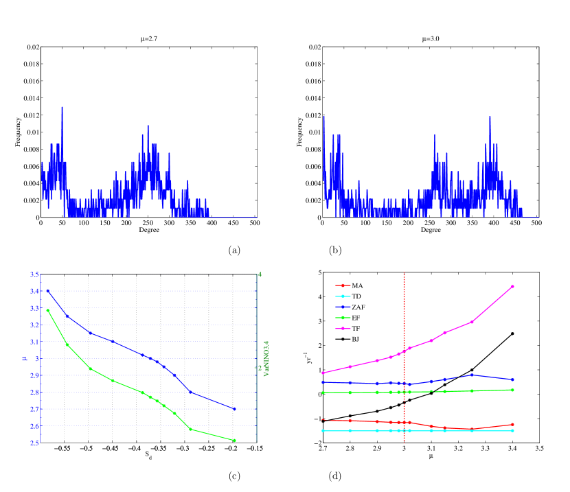
Figure 2: (a) Degree distribution of the PCCN using a threshold $\tau=0.5$ reconstructed from the modified ZC model data at the coupling strength $\mu=2.7$. (b) Same as (a) but at the coupling strength $\mu=3.0$. (c) The degree skewness index $S_{d}$ from the modified ZC model as a function of the coupling strength $\mu$ (blue) and the variance of NINO3.4 index $Var_{NINO3.4}$ (green). (d) The values of BJ index and its components from the modified ZC model at different coupling strength $\mu$ ($\mu_{c}=3.0$, red dash line): mean advection and upwelling (MA, red), thermal damping (TD, cyan), zonal advection feedback (ZAF, dark blue), Ekman pumping feedback (EF, green), thermocline feedback (TF, magenta), and total BJ index (BJ, black).

To validate the new index $S_{d}$, we use the results from a fully-coupled ZC model [22]. In its standard setup, the Hopf bifurcation occurs at $\mu_{c}=3.0$ (Supplementary Fig. 2). Time series of the SST field are generated using an additional red-noise wind forcing [20] (see Methods and section 3 in SI for details on the model and the red noise product) for different values of $\mu$ between $2.7$ and $3.4$. From each 540-month (45-year) simulations the degree fields of the networks reconstructed are shown in Fig. 1 for four values of $\mu$. When the coupling strength $\mu$ is increased from the subcritical $\mu<\mu_{c}$ to the supercritical regime $\mu>\mu_{c}$, more nodes in the region between 220^∘E and 280^∘E get a higher degree. When the critical boundary is approached, the spatial pattern of the anomalies is more and more controlled by the ENSO mode, leading to large-scale coherence which is efficiently measured by the network degree field. Another distinct change of the degree fields (Fig. 1a-1d) is that the propagating patterns of equatorially symmetric Rossby waves are becoming more prominent when the background state enters the supercritical regime.

Histograms of the degree fields (the degree distributions) for two different values of $\mu$ are plotted in Fig. 2a-2b. For $\mu=2.7<\mu_{c}$ (Fig. 2a), the degree distribution is bimodal, where the first peak represents the low degree nodes in Fig. 1a and the second peak (located near 250) represents the high degree nodes. When $\mu$ is increased (Fig. 2b) a peak at even higher degree occurs because the ENSO mode becomes more dominant in the SST anomalies when the background climate moves into the supercritical regime [25, 11]. The skewness of the degree distribution $S_{d}$ is monotonically decreasing with increasing $\mu$ (blue curve in Fig. 2c). There is also a good correlation between $S_{d}$ and the variance of the NINO3.4 index ($Var_{NINO3.4}$, green curve) as shown in Fig. 2c. However, note that under high values of $S_{d}$ (stable climate, $\mu<\mu_{c}$), the amplitude of NINO3.4 depends on the noise (cf. Supplementary Fig. 1).

For the ZC-model results here, the BJ index (the black curve in Fig. 2d, details of the calculation can be found in section 4 of the SI) is monotonously increasing with increasing $\mu$ and crosses the zero line at about $\mu=3.1$ which is close to $\mu_{c}$. This indicates that the BJ index reasonably (but not perfectly) monitors the stability of the background state for this case, which is in accordance with results in Jin et al. [5]. The values of different terms in the BJ index (also shown in Fig. 2d) indicate that the thermocline feedback is dominant in destabilizing the background state. It has been shown in models [7, 8] and reanalysis data [8] that this feedback has been dominant during past ENSO events.

Next, we reconstruct PCCNs for the observed SST data (the HadISST dataset [26]) and focus on two major ENSO events over the last 60 years, which peaked in 1982 and 1997. To show the different network properties for these individual ENSO events, we used monthly SST data of 4 years surrounding the peak of the event (two years before and one year after the year in which the peak occurred). Figure 3a-3b indicate that the degree fields of the PCCNs reconstructed for these two major ENSO events are substantially different. The pattern for the 1997 event displays a much larger area of high degree than that of the 1982 event which is more localized and has a smaller degree. Comparing these to the patterns in Fig. 1, one would interpret the (1982) 1997 event to be in the (sub) supercritical regime.

To monitor the changes in the stability of the Pacific climate, we applied the stability index $S_{d}$ to the HadISST dataset from December 1951 to November 2014 (63 years). We reconstructed a PCCN for every 10 years of monthly SST data and computed its $S_{d}$. By implementing a sliding-window strategy with a shift of one month, we obtained a time series of $S_{d}$ (black curve in Fig. 3c), showing the variation of the stability over the Pacific background climate over the last 60 years. The 3-month running mean of NINO3 index of the same period is plotted as the green curve in Fig. 3c. We also marked the $S_{d}$ values of the 1982 and 1997 events, clearly indicating that the $S_{d}$ value at the onset of the 1982 ENSO event (January-March value of $S_{d}=0.03$ in 1982) is much higher than the one for the 1997 event (January-March value of $S_{d}=-0.37$ in 1997). Actually, the value of $S_{d}$ was overall low during the early 90s with a global minimum just before the 1997 event. The high value of $S_{d}$ early 1982 indicates that noise must have had a large influence on the development of the 1982 El Niño event. The noise product (see Methods) from the Florida State University wind stress indeed indicates that high noise variability was present during this time (See section 3 of the SI, in particular Supplementary Fig. 3).

In summary, using techniques of complex network theory we have developed a novel index $S_{d}$ which provides a simple and adequate measure of the stability of the Pacific climate both in models and observations. From Fig. 3c, it is interesting to see that the $S_{d}$ index increased in the beginning of the year 2014, indicating that the Pacific climate became more stable. This is consistent with the fact that although large subsurface temperature anomalies developed in March 2014, there was no growth of SST anomalies because the thermocline feedback was weak and no strong El Niño event could develop. In this way, our new index can provide an additional tool which can help improve El Niño predictions in the future.

Methods

• Model: The model used for this study is a fully-coupled variant of the original Zebiak-Cane (ZC) model [22]. The ocean component of this model is a reduced-gravity shallow-water model, and the atmospheric component is a linear, steady-state model [27] forced by the sea-surface temperature (SST). In contrast to the original ZC model, this model is not an anomaly model around a prescribed climatological mean state, but the model itself generates the mean climate state and its variability. More detailed information on this model can be found in Dijkstra and Neelin [28] and van der Vaart et al. [22]. We use model output of 11 simulations at different values of the coupling strength $\mu$, (2.70, 2.80, 2.90, 2.95, 2.98, 3.00, 3.02, 3.10, 3.15, 3.25, 3.40).

• Red Noise: We followed the same procedure of introducing the red noise into the wind-stress forcing in the model as in Roulston and Neelin [20]. We used the reconstructed data of Pacific SST for the period of 1978-2004 [29], and the Florida State University pseudo-wind-stress data for the same period [30]. Details of the construction of the noise product and its effect on the behavior of the ENSO variability in the ZC model is given in section 3 of the SI.

• Network Reconstruction: We reconstruct Climate Networks (CNs) for SST data sets both from the model output and observations (HadISST dataset [26]). The model SST output is considered on a domain of (140^∘E, 280^∘E) $\times$ (20^∘S, 20^∘N) on a 30 $\times$ 31 grid, which provides a time series of 540 monthly SST anomaly fields (with respect to the time mean). The nodes of the each CN are the grid points where we have the SST data. A ‘link’ between two nodes is determined by a significant correlation between their SST anomaly time series measured here by the Pearson correlation [9]. For this study, each PCCN consists of 30 (longitude)$\times$31 (latitude)$=930$ nodes, and as a threshold for significance ($p<0.05$) we choose the threshold value $\tau=0.5$ .

Correspondence

Correspondence and requests for materials should be addressed to Q. Y. Feng (email: Q.Feng@uu.nl).

Author contribution

Both authors designed the study, Q. Y. Feng performed most of the analysis, and both authors contributed to the writing of the paper.

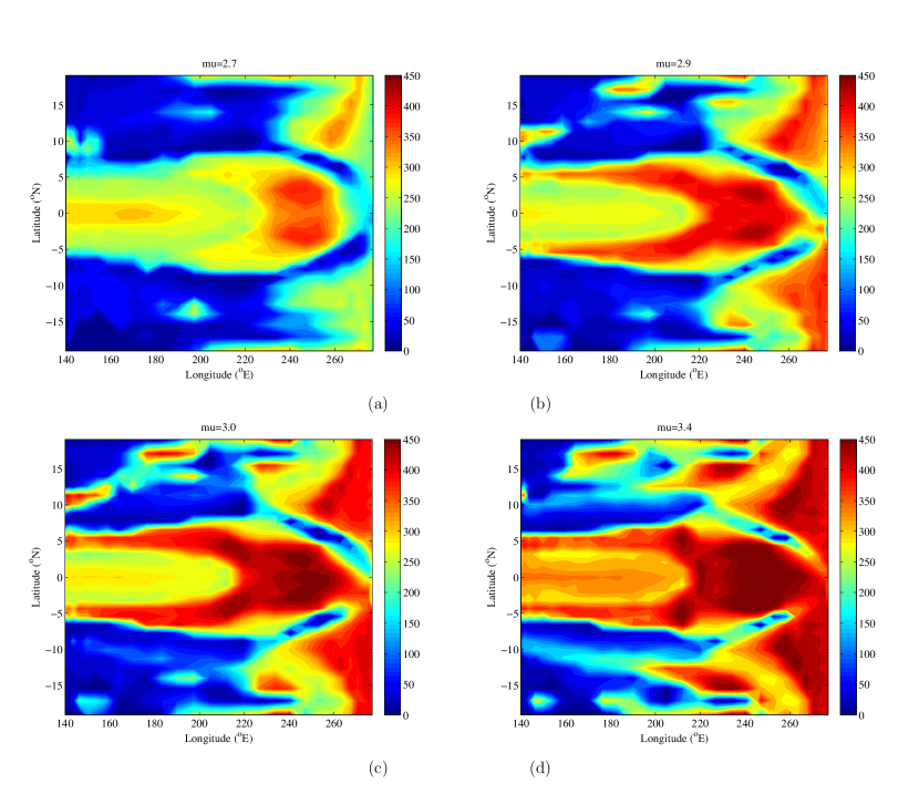
Figure 1: (a) Degree field of the Pearson Correlation Climate Network (PCCN) using a threshold $\tau=0.5$ reconstructed from the modified ZC model data at the coupling strength $\mu=2.7$. (b) Same as (a) but at the coupling strength $\mu=2.9$. (c) Same as (a) but at the coupling strength $\mu=3.0$. (d) Same as (a) but at the coupling strength $\mu=3.4$.

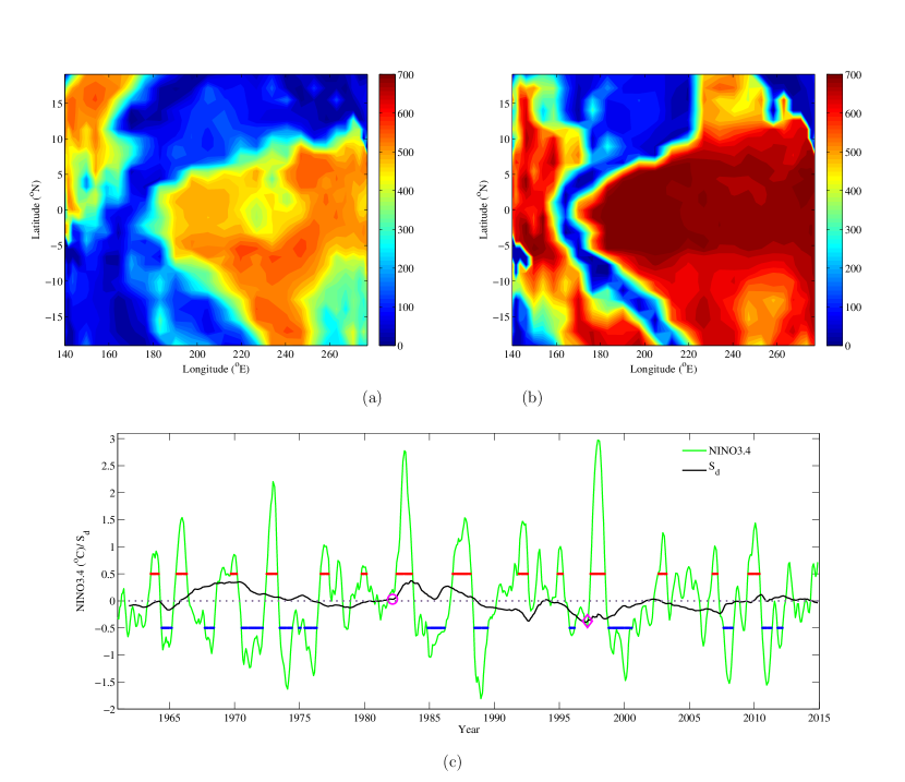
Figure 3: (a) Degree field of the PCCN using a threshold $\tau=0.5$ reconstructed from the observed SST of Jan 1980 to Dec 1983. (b) Same as (a) but of the observed SST of Jan 1995 to Dec 1998. (c) The 10-year sliding window degree skewness index $S_{d}$ (balck curve) and the 3-month running NINO3.4 index (green curve) from the observed SST of Dec 1951 to Nov 2014. The x-axis indicates the end time of the sliding window. The magenta circle indicates the mean $S_{d}$ value of the window ending at January-March 1982, and the magenta diamond indicates that of January-March 1997. The red (blue) lines indicate El Niño (La Niña) events that a five consecutive 3-month running mean of NINO3.4 index that is above (below) the threshold of $+0.5^{\circ}$C ($-0.5^{\circ}$C).

References

- [1] Climate Diagnostics Bulletin (National Oceanic and Atmospheric Administration, National Weather Service, Climate Prediction Center). URL www.cpc.ncep.noaa.gov/products/CDB.
- [2] Fedorov, A., Harper, S., Philander, S., Winter, B. & Wittenberg, A. How predictable is el niño? Bulletin of the American Meteorological Society 84, 911–919 (2003).
- [3] Chen, D., Cane, M. A., Kaplan, A., Zebiak, S. E. & Huang, D. Predictability of el niño over the past 148 years. Nature 428, 733–736 (2004).
- [4] Yeh, S.-W. et al. El Niño in a changing climate. Nature 461, 511–514 (2009).
- [5] Jin, F.-F., Kim, S. T. & Bejarano, L. A coupled-stability index for ENSO. Geophysical Research Letters 33 (2006).
- [6] Kim, S. T. & Jin, F.-F. An ENSO stability analysis. part i: Results from a hybrid coupled model. Climate Dynamics 36, 1593–1607 (2011).
- [7] Kim, S. T. & Jin, F.-F. An ENSO stability analysis. part ii: Results from the twentieth and twenty-first century simulations of the cmip3 models. Climate Dynamics 36, 1609–1627 (2011).
- [8] Kim, S. T. et al. Response of El Nino sea surface temperature variability to greenhouse warming. Nature Climate Change (2014).
- [9] Tsonis, A. A. & Swanson, K. L. What do networks have to do with climate? Bulletin Of The American Meteorological Society 87, 585–595 (2006).
- [10] Donges, J. F., Zou, Y., Marwan, N. & Kurths, J. Complex networks in climate dynamics. The European Physical Journal Special Topics 174, 157–179 (2009).
- [11] Feng, Q. Y., Viebahn, J. P. & Dijkstra, H. A. Deep ocean early warning signals of an Atlantic MOC collapse. Geophysical Research Letters 41 (2014).
- [12] Zebiak, S. E. & Cane, M. A. A model El Niño-Southern Oscillation. Monthly Weather Review 115, 2262–2278 (1987).
- [13] Neelin, J. et al. ENSO Theory. Journal of Geophysical Research 103, 14,261–14,290 (1998).
- [14] Jin, F.-F. An equatorial recharge paradigm for ENSO. II: A stripped-down coupled model. J. Atmos. Sci. 54, 830–8847 (1997).
- [15] Fedorov, A. V. & Philander, S. G. Is El Niño Changing? Science 288, 1997–2002 (2000).
- [16] Bejarano, L. & Jin, F.-F. Coexistence of equatorial coupled modes of ENSO. Journal of Climate 21, 3051–3067 (2008).
- [17] Penland, C. A stochastic model of IndoPacific sea surface temperature anomalies. Physica D: Nonlinear Phenomena 98, 534–558 (1996).
- [18] Burgers, G. The El Niño Stochastic Oscillator. Clim. Dyn. 15, 352–375 (1999).
- [19] Jin, F.-F., Neelin, J. & Ghil, M. El Niño/Southern Oscillation and the annual cycle: Subharmonic frequency-locking and aperiodicity. Physica D-Nonlinear Phenomena 98, 442–465 (1996).
- [20] Roulston, M. & Neelin, J. The response of an ENSO model to climate noise, weather noise and intraseasonal forcing. Geophys. Res. Letters 27, 3723–3726 (2000).
- [21] Dijkstra, H. A. Nonlinear Climate Dynamics (Cambridge University Press, New York, U.S.A., 2013).
- [22] Van der Vaart, P. C. F., Dijkstra, H. A. & Jin, F.-F. The Pacific Cold Tongue and the ENSO mode: Unified theory within the Zebiak-Cane model. J. Atmos. Sci. 57, 967–988 (2000).
- [23] Gozolchiani, A., Havlin, S. & Yamasaki, K. Emergence of El Niño as an Autonomous Component in the Climate Network. Physical Review Letters 107, 148501 (2011).
- [24] Ludescher, J. et al. Improved el niño forecasting by cooperativity detection. Proceedings of the National Academy of Sciences 110, 11742–11745 (2013).
- [25] Mheen, M. et al. Interaction network based early warning indicators for the Atlantic MOC collapse. Geophysical Research Letters 40, 2714–2719 (2013).
- [26] Rayner, N. A. et al. Global analyses of sea surface temperature, sea ice, and night marine air temperature since the late nineteenth century. Journal of Geophysical Research 108, 10.1029/2002JD002670 (2003).
- [27] Gill, A. E. Some simple solutions for heat induced tropical circulation. Quart. J. Roy. Meteor. Soc. 106, 447–462 (1980).
- [28] Dijkstra, H. A. & Neelin, J. Coupled ocean-atmosphere models and the tropical climatology. II: Why the cold tongue is in the east. J Climate 8, 1343–1359 (1995).
- [29] Smith, T. M., Reynolds, R. W., Livezey, R. E. & Stokes, D. C. Reconstruction of historical sea surface temperatures using empirical orthogonal functions. Journal of Climate 9, 1403–1420 (1996).
- [30] Legler, D. & O’Brien, J. 2. Tropical Pacific wind stress analysis for toga. Intergovernmental Oceanographic Commission 11 (1988).