Signatures of pairing and spin-orbit coupling in correlation functions of Fermi gases

Abstract

We derive expressions for spin and density correlation functions in the (greatly enhanced) pseudogap phase of spin-orbit coupled Fermi superfluids. Density-density correlation functions are found to be relatively insensitive to the presence of these Rashba effects. To arrive at spin-spin correlation functions we derive new $f$-sum rules, valid even in the absence of a spin conservation law. Our spin-spin correlation functions are shown to be fully consistent with these $f$-sum rules. Importantly, they provide a clear signature of the Rashba band-structure and separately help to establish the presence of a pseudogap.

Introduction.$-$ Spin-orbit coupling (SOC) in superconductors and superfluids is a topic of much current interest Hasan and Kane (2010); Zhang et al. (2008); Sato et al. (2009). This is in large part because there is some hope that (particularly in the presence of a magnetic field) they may relate to the much sought after spinless $p_{x}+ip_{y}$ superfluid Read and Green (2000). Two communities have united around these issues: those working on cold Fermi superfluids with intrinsic Rashba SOC Zhai (2015); Goldman et al. (2014) and those studying superconductivity that is proximity induced in a spin-orbit coupled material Fu and Kane (2008). To achieve this ultimate goal it is important to establish that a given candidate for the $p_{x}+ip_{y}$ superfluid simultaneously exhibits signatures of both pairing and spin orbit coupling. This would provide minimal evidence for a properly engineered ultracold atomic gas. One therefore needs experimental signatures of these simultaneous effects and this provides a central goal for the present paper.

Here we address the signatures of this anomalous spin-orbit coupled superfluid as reflected in spin-spin and density-density correlation functions. Our work builds on the observation  Vyasanakere et al. (2011); Vyasanakere and Shenoy (2011); Yu and Zhai (2011); Hu et al. (2011); Gong et al. (2011); Han and Sá de Melo (2012) that in the presence of Rashba SOC, pairing (in the form of pseudogap effects Chen et al. (2005); Stajic et al. (2004)) is significantly enhanced. For this reason (and because the correlation functions are free of the complications of collective mode effects) we focus here on the normal phase. We show how even without condensation, the frequency dependent spin response exhibits features which relate to the Rashba ring band-structure, as well as to the presence of a pairing gap. In contrast, the density response is relatively unaffected by SOC. Previous work has focused on identifying SOC without Cheuk et al. (2012); Wang et al. (2012) or with pairing Fu et al. (2013) via the one body spectral function. As compared with Ref. Fu et al. (2013), we find less subtle features in the two particle response. At the very least the spin correlation functions provide complementary and accessible (via neutrons or two photon Bragg scattering Veeravalli et al. (2008)) information.

Validating any theory of correlation functions requires satisfying important constraints Boyack et al. (2014). Indeed, the absence of conservation laws complicates all spin transport in spin-orbit coupled materials. Thus, it is extremely important to find underlying principles for establishing self consistency. To address this issue, here we use the Heisenberg equations of motion to derive $f$-sum rules for the spin-spin correlation functions, which also provides important constraints on our numerical calculations. While a magnetic field is necessary for arriving at topological order, we begin by ignoring this additional complication. There is a substantial literature investigating correlation functions in the superfluid phase (without pseudogap effects) which we note here Ojanen and Kitagawa (2013); Chung and Roy (2014); Roy and Kallin (2008); Lutchyn et al. (2008).

In this Rapid Communication we present two main results. The first is a consistent derivation of spin-spin correlation functions in spin-orbit coupled Fermi gases. The second establishes qualitative experimental signatures reflecting separately the presence of a pairing gap and of SOC. Readers interested in the experimental signatures need only a cursory exploration of the mathematical derivation that precedes it.

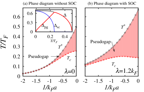
Figure 1: Phase diagrams for a degenerate fermi gas without (a) and with (b) SOC. Plotted is $T^{*}$ as a function of inverse scattering length, $1/k_{F}a$, indicating where pairing first sets in, while $T_{c}$ marks the onset of condensation to the superfluid phase. The plot shows the weakly interacting regime with $1/k_{F}a<0$. As spin-orbit coupling is turned on, pairing is enhanced leading to a larger pseudogap region. The inset in (a) indicates the temperature dependences of the component gap parameters (defined in the text) at unitarity, $1/k_{F}a=0$.

Background Theory.$-$ We consider a gas of fermions whose single particle Hamiltonian is $H^{0}({\bf k})=k^{2}/2m-\mu+\lambda\boldsymbol{\sigma}\cdot{\bf k}_{\perp}/m$ for a particle of mass $m$, spin-orbit coupling momentum $\lambda$, momentum ${\bf k}=(k_{x},k_{y},k_{z})$, in-plane momentum ${\bf k}_{\perp}=(k_{x},k_{y},0)$, and vector of Pauli matrices $\boldsymbol{\sigma}=(\sigma_{x},\sigma_{y},\sigma_{z})$. Throughout this paper we set $\hbar=k_{B}=1$. To describe our spin-orbit coupled Fermi gas with pairing, we use a $4\times 4$ inverse Nambu Green’s function

$$\mathcal{G}^{-1}(K)=\begin{pmatrix}G_{0}^{-1}(K)&\Delta\\ \Delta&\widetilde{G}_{0}^{-1}(K)\end{pmatrix},$$ (1)

that acts on the spinor $\Psi_{\bf k}^{T}=\left(c_{{\bf k}\uparrow},c_{{\bf k}\downarrow},-c^{\dagger}_{-{\bf k}\downarrow},c^{\dagger}_{-{\bf k}\uparrow}\right)$ for a fermion annihilation (creation) operator $c_{{\bf k}s}(c_{{\bf k}s}^{\dagger})$ of spin $s=\uparrow,\downarrow$ and momentum ${\bf k}$. In the Green’s function $\Delta$ is a pairing gap, the 4-vector $K=(i\omega,\mathbf{k})$ with Matsubara frequency $i\omega$, and the non-interacting inverse particle Green’s function is $G_{0}^{-1}(K)=i\omega-H^{0}({\bf k})$ and hole Green’s function $\widetilde{G}_{0}^{-1}(K)=i\sigma_{y}[G_{0}^{-1}(-K)]^{T}i\sigma_{y}=i\omega+H^{0}({\bf k})$.

This superfluid can be studied at the mean field level Vyasanakere et al. (2011); Vyasanakere and Shenoy (2011); Yu and Zhai (2011); Hu et al. (2011); Gong et al. (2011); Han and Sá de Melo (2012), where one has the usual gap equation:

$$1=\frac{g}{2}\sum_{K}\mathrm{Tr}\left[G(K)\widetilde{G}_{0}(K)\right],$$ (2)

where $\sum_{K}=T\sum_{i\omega}\sum_{\bf k}$ is a sum over momentum and Matsubara frequencies at temperature $T$, and where the many-body Green’s function $G(K)$ is found from the inverse of Eq. (1)

$$G^{-1}(K)-G_{0}^{-1}(K) = -\Sigma(K)=-\Delta^{2}\widetilde{G}_{0}(K).$$ (3)

Except for the matrix structure in the above equations, these are the usual definitions of the fermionic Green’s functions and self energy associated with BCS theory; the gap equation also appears in the literature Vyasanakere et al. (2011); Vyasanakere and Shenoy (2011); Yu and Zhai (2011); Hu et al. (2011); Gong et al. (2011); Han and Sá de Melo (2012). As in the cold atoms literature, we will regularize the gap equation by replacing the interaction strength $g$ with the scattering length $a$ through $1/g=m/4\pi a-1/V\sum_{\textbf{k}}m/\textbf{k}^{2}$.

We now want to include pair fluctuations, or pseudogap (pg) effects, in a fashion fully consistent with both the ground state and the mean field equations that have been extensively studied in previous work Vyasanakere et al. (2011); Vyasanakere and Shenoy (2011); Yu and Zhai (2011); Hu et al. (2011); Gong et al. (2011); Han and Sá de Melo (2012). The approach we outline below was introduced in the context of high temperature superconductors Chen et al. (2005, 1998), but it has also been applied to spin-orbit coupled superfluids He et al. (2013).

Pair fluctuations lower the phase transition temperature $T_{c}$ relative to its mean field value denoted by $T^{*}$. The latter is the temperature at which the pairing gap, determined by Eq. (2), first becomes non zero. (Note that $T^{*}$ does not reflect a broken symmetry state and is not a true phase transition). As a result, a central component of the present theory is that the usual Thouless condition (on the $t$-matrix) for the instability of the normal phase Schrieffer (1964) must be modified to include a well developed excitation gap.

Imposing consistency with mean field theory for the pairing gap obtained from Eq. (2) leads to a modified Thouless condition:

$$t_{{\mathrm{pg}}}(Q)\equiv\frac{g}{1+g\raisebox{1.50696pt}{$\chi$}(Q)}\rightarrow\infty,\text{\ as\ }Q\rightarrow 0,$$ (4)

where

$$\raisebox{1.50696pt}{$\chi$}(Q)\equiv-\frac{1}{2}\sum_{K}\mathrm{Tr}\left[G(K)\widetilde{G}_{0}(K-Q)\right].$$ (5)

In this way, above $T_{c}$ the square of the excitation gap of the non-condensed pairs, called $\Delta_{{\mathrm{pg}}}^{2}$, is to be associated with $\Delta^{2}$, given by Eq. (2) . Establishing $T_{c}$, however, requires that we find a constraint on $\Delta_{{\mathrm{pg}}}^{2}$ applicable at and below $T_{c}$. Indeed, once $T<T_{c}$, there must be another contribution to the self energy $\Sigma(K)$ involving $Q=0$ or superconducting (sc) pairs. Then the self energy of Eq. (3) can be written in terms of a $t$-matrix (as in the Thouless condition) $\Sigma(K)=-\sum_{Q}t(Q)\widetilde{G}_{0}(K-Q),$ Chen et al. (1998): $t_{{\mathrm{pg}}}(Q)+t_{{\mathrm{sc}}}(Q)$, where $t_{{\mathrm{sc}}}(Q)\equiv-\frac{\Delta_{{\mathrm{sc}}}^{2}}{T}\delta(Q)$ represents the condensate. As a consequence $\Sigma(K)=\Sigma_{{\mathrm{sc}}}(K)+\Sigma_{{\mathrm{pg}}}(K)$. Because of Eq. (4), the quantity $t_{{\mathrm{pg}}}(Q)$ is strongly peaked at $Q=0$ and $\Sigma_{{\mathrm{pg}}}(K)\approx\Delta_{{\mathrm{pg}}}^{2}\widetilde{G}_{0}(K)$.

This relation implies that $\Delta_{{\mathrm{pg}}}^{2}=-\sum_{Q\neq 0}t_{{\mathrm{pg}}}(Q)$, or equivalently, the pseudogap is approximated as a thermal gas of composite bosons. The transition temperature $T_{c}$ is determined as the temperature at which this value of $\Delta_{{\mathrm{pg}}}$, when the transition is approached from below, intersects with the mean field gap equation, which corresponds to $\Delta_{{\mathrm{pg}}}$ above $T_{c}$ in the normal state. In this way, in the ordered phase the total self energy $\Sigma(K)=\Delta^{2}\widetilde{G}_{0}(K)$, where $\Delta^{2}=\Delta_{{\mathrm{sc}}}^{2}+\Delta_{{\mathrm{pg}}}^{2}$. In the inset of Fig. 1(a), we plot the temperature dependence for both $\Delta_{{\mathrm{sc}}}$ and $\Delta_{{\mathrm{pg}}}$, as well as the total excitation gap $\Delta$.

We emphasize that a central distinguishing feature of the present approach is that $T_{c}$ is determined in the presence of a well developed gap at $T_{c}$. This contrasts with the scheme of Nozieres and Schmitt-Rink Nozières and Schmitt-Rink (1985) and is similarly different from path integral-collective mode schemes He and Huang (2013). The latter introduce Goldstone bosons, but importantly these do not renormalize the mean field transition temperature which remains at $T^{*}$.

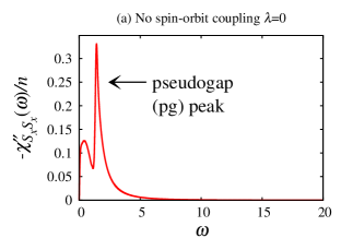
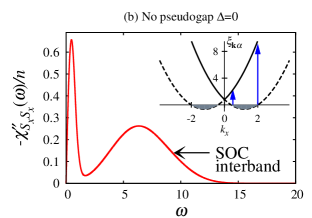
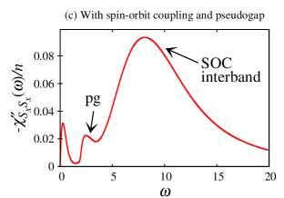
Figure 2: The spin-spin response function as a function of frequency. Figure 2(a) corresponds to a pseudogap phase without SOC. The peak at lower $\omega$ reflects thermally excited fermions while the second peak is at $\omega$ comparable to the pseudogap energy scale, where pairs are now broken. Since $\lambda=0$, the spin-spin and density-density correlation functions are the same. In Fig. 2(b) the pseudogap is set to zero with fixed $\lambda=1.2k_{F}$. The lower energy intra-helicity band peak is enhanced and one sees an SOC-related peak. As shown in the inset, the low-energy threshold reflects the onset of inter-helicity band transitions, while the high-energy endpoint occurs when these transitions are no longer possible. In Fig. 2(c), in the presence of both a pseudogap and SOC, one sees a combination of the effects in the previous two panels. Spectral weight is transferred to yield a larger SOC peak, reflecting the gapping of the low energy contributions. All quantities are measured relative to the Fermi energy, $E_{F}$, or Fermi momentum $k_{F}$.

Figure 1 shows the calculated phase diagram, plotting $T_{c}$ and $T^{*}$, in the absence (a) and presence (b) of Rashba SOC. The latter is in reasonable agreement with the results of Ref. He et al. (2013). We restrict these plots to the weak pairing side of resonance. Here we observe a greatly enhanced pseudogap regime denoted by an enhancement of $T^{*}$ without significant enhancement of $T_{c}$. The behavior of $T^{*}$ has been attributed to the enhancement of the pairing attraction Vyasanakere et al. (2011); Vyasanakere and Shenoy (2011); Yu and Zhai (2011); Hu et al. (2011); Gong et al. (2011); Han and Sá de Melo (2012), due to an increased density of states near the minimum of the Rashba ring. Since $T_{c}$ is obtained in the presence of a gap at $T_{c}$, stronger pairing (reflected in $T^{*}$) is offset by an increasingly gapped density of states. This leads to a relatively constant $T_{c}$ as a function of interaction strength.

Density/current and $f$-sum rules.$-$ To characterize the anomalous, normal, and superfluid phases in more detail, we investigate both the density/current and spin correlation functions, considering the former first. For systems with a $U(1)$ symmetry, the Ward-Takahashi identity (WTI) provides an important constraint on the full vertex $\Gamma^{\mu}(\widetilde{K},K)$ which enters into the correlation functions. Given a mean field like self energy, it is possible to analytically solve the WTI, and obtain the full vertex function along with the full correlation function Schrieffer (1964); Boyack et al. (2014).

We define the generalized correlation function

$$P^{\mu\nu}(Q)=\sum_{K}\mathrm{Tr}\left[G(\widetilde{K})\Gamma^{\mu}(\widetilde{K},K)G(K)\gamma^{\nu}(K,\widetilde{K})\right],$$ (6)

where $\widetilde{K}\equiv K+Q$ and $\gamma^{\mu}(\widetilde{K},K)$ is a bare vertex. From this we have the density-density $\raisebox{1.50696pt}{$\chi$}_{\rho\rho}(Q)\equiv P^{00}(Q)$ and current-current correlation functions $\tensor{\raisebox{1.50696pt}{$\chi$}}_{JJ}(Q)\equiv P^{ij}(Q),i,j\in\{1,2,3\}$. The bare and full vertices satisfy respectively

$$q_{\mu}\gamma^{\mu}(\widetilde{K},K) = G_{0}^{-1}(\widetilde{K})-G_{0}^{-1}(K),$$ (7)

$$q_{\mu}\Gamma^{\mu}(\widetilde{K},K) = G^{-1}(\widetilde{K})-G^{-1}(K),$$ (8)

with the latter a consequence of the WTI. We now specialize to systems with the self energy as in Eq. (3). Using the WTI above $T_{c}$ we have

$$\Gamma^{\mu}(\widetilde{K},K)=\gamma^{\mu}(\widetilde{K},K)+\Delta^{2}\widetilde{G}_{0}(\widetilde{K})\widetilde{\gamma}^{\mu}(\widetilde{K},K)\widetilde{G}_{0}(K),$$ (9)

where $\widetilde{\gamma}^{\mu}(\widetilde{K},K)=\sigma_{y}{\gamma}^{\mu}(-\widetilde{K},-K)^{T}\sigma_{y}$ is a time-reversed vertex. Inserting the full vertex into Eq. (6) then gives the correlation functions above $T_{c}$.

One can incorporate superconducting (or equivalently superfluid) terms within this formalism building on Eq. (9) and, for example, address the superfluid density Chen et al. (1998), as outlined in the supplement. One considers the transverse response $P_{T}^{\mu\nu}(Q)$ which contains no collective modes:

$$P_{T}^{\mu\nu}(Q) = \sum_{K}\mathrm{Tr}\biggl{\{}\left[G(\widetilde{K})\gamma^{\mu}(\widetilde{K},K)G(K)\right.$$ (10)

$$+ {F}_{{\mathrm{pg}}}(\widetilde{K})\widetilde{\gamma}^{\mu}(\widetilde{K},K)\widetilde{{F}}_{{\mathrm{pg}}}(K)$$

$$- \left.F_{{\mathrm{sc}}}(\widetilde{K})\widetilde{\gamma}^{\mu}(\widetilde{K},K)\widetilde{F}_{{\mathrm{sc}}}(K)\right]\gamma^{\nu}(K,\widetilde{K})\biggr{\}},$$

where $F_{m}(K)=\Delta_{m}\widetilde{G}_{0}(K)G(K)=\widetilde{F}_{m}(K)$ for $m\in\{{\mathrm{sc}},{\mathrm{pg}}\}$. Note that $F_{{\mathrm{pg}}}$ does not represent an anomalous Green’s function, but rather reflects a vertex correction to the correlation functions Boyack et al. (2014). There is a disagreement in the literature Ojanen and Kitagawa (2013); Hu et al. (2011) as to the importance of collective modes in the spin response below $T_{c}$. We agree with the results of Ref. Ojanen and Kitagawa (2013), where collective modes were included.

As shown in the supplementary material, when one integrates over the entire frequency range, a consequence of the WTI is that the $f$-sum rule is satisfied:

$$\int\frac{d\omega}{\pi}\left(-\omega\raisebox{1.50696pt}{$\chi$}^{\prime\prime}_{\rho\rho}(\omega,{\bf q})\right)=\frac{nq^{2}}{m},$$ (11)

where $\raisebox{1.50696pt}{$\chi$}^{\prime\prime}_{\rho\rho}$ is the imaginary part of the density response function. This $f$-sum rule depends on the total particle number $n$ and the bare mass $m$. Since $\lambda$ does not enter, the presence of spin-orbit coupling does not modify the weight of the $f$-sum rule.

Spin response and $f$-sum rules.$-$ In the spin channel, where there is no $U(1)$ symmetry to justify the use of the WTI. Nevertheless, we are able to provide an a posteriori check on any proposed correlation function via a sum rule which we now derive. We define $\raisebox{1.50696pt}{$\chi$}_{S_{i}S_{j}}\left(i\omega,\mathbf{q}\right)\equiv\int d\tau\,e^{i\omega\tau}\left\langle T_{\tau}S_{\mathbf{q}i}\left(\tau\right)S_{-\mathbf{q}j}\left(0\right)\right\rangle$ where $T_{\tau}$ is the time ordering operator and $S_{\mathbf{q}i}=\sum_{\mathbf{k}ss^{\prime}}c_{\mathbf{k}s}^{\dagger}\left(\sigma_{i}\right)_{ss^{\prime}}c_{\mathbf{k}+\mathbf{q}s^{\prime}}$ is the many-body spin density operator. Using the Heisenberg equations of motion and the properties of Fourier transforms, the sum rule for the spin-spin correlation function $\raisebox{1.50696pt}{$\chi$}^{\prime\prime}_{S_{i}S_{j}}$ can be shown to be

$$\int\frac{d\omega}{\pi}\left(-\omega\raisebox{1.50696pt}{$\chi$}^{\prime\prime}_{S_{i}S_{j}}\left(\omega,\mathbf{q}\right)\right) = \left\langle\left[\left[\mathcal{H}_{0},S_{\mathbf{q}i}\right],S_{-\mathbf{q}j}\right]\right\rangle,$$ (12)

where $\mathcal{H}_{0}=\sum_{ss^{\prime}\mathbf{k}}c_{\mathbf{k}s}^{\dagger}H^{0}_{ss^{\prime}}\left(\mathbf{k}\right)c_{\mathbf{k}s^{\prime}}$ and $\raisebox{1.50696pt}{$\chi$}^{\prime\prime}_{S_{i}S_{j}}$ is the singular part of $\raisebox{1.50696pt}{$\chi$}_{S_{i}S_{j}}$ found by analytically continuing $i\omega\rightarrow\omega+i\delta$ and then taking the $\delta\rightarrow 0$ limit.

Here we give the explicit result, for two example cases of interest and present further details in the supplementary material:

$$\int\frac{d\omega}{\pi}\left(-\omega\raisebox{1.50696pt}{$\chi$}^{\prime\prime}_{S_{i}S_{i}}\left(\omega,\mathbf{q}\right)\right) =\frac{nq^{2}}{m}-\frac{4\lambda}{m}\sum_{\mathbf{k}\alpha}\alpha f_{ii}n_{\mathbf{k}\alpha}.$$ (13)

where $i\in\{x,z\}$, $f_{zz}=k_{\perp}$, $f_{xx}=k_{x}^{2}/k_{\perp}$ and $n_{\mathbf{k}\alpha}=T\sum_{i\omega}G^{\alpha}_{H}(K),$ with $G^{\alpha}_{H}(K)$ a helicity Green’s functions to be defined in the next section.

Correlation functions in the helicity basis.$-$ In the absence of a magnetic field, helicity is a good quantum number, and the correlation functions are most easily expressed in terms of the helicity Green’s functions He et al. (2013):

$$G_{H}^{\alpha}(K) \equiv \frac{u_{\mathbf{k}\alpha}^{2}}{i\omega-E_{\mathbf{k}\alpha}}+\frac{v_{\mathbf{k}\alpha}^{2}}{i\omega+E_{\mathbf{k}\alpha}},$$ (14)

$${F}_{H}^{\alpha}(K) \equiv u_{\mathbf{k}\alpha}v_{\mathbf{k}\alpha}\left(\frac{1}{i\omega+E_{\mathbf{k}\alpha}}-\frac{1}{i\omega-E_{\mathbf{k}\alpha}}\right),$$ (15)

where $E_{\mathbf{k}\alpha}=\sqrt{\xi^{2}_{\mathbf{k}\alpha}+\Delta^{2}}$, $\xi_{\mathbf{k}\alpha}=k^{2}/2m-\mu+\alpha\lambda k_{\perp}/m$ is an eigenvalue of $H^{0}({\bf k})$, and ${F}^{\alpha}_{H}(K)$ represents the pseudogap, or equivalently vertex contribution. Here $\alpha=\pm$ denotes the helicity index and the coherence factors satisfy $u_{\mathbf{k}\alpha}^{2}=\tfrac{1}{2}(1+\xi_{\mathbf{k}\alpha}/E_{\mathbf{k}\alpha})$, $u_{\mathbf{k}\alpha}^{2}+v_{\mathbf{k}\alpha}^{2}=1.$

It follows from the vertex function in Eq. (9) that the explicit form for the $f$-sum rule Boyack et al. (2014) consistent density-density correlation function is

$$\raisebox{1.50696pt}{$\chi$}_{\rho\rho}(\omega,{\bf q})=\frac{1}{2}\sum_{K,\alpha,\alpha^{\prime}}\left(1+\alpha\alpha^{\prime}\cos\left(\phi_{\bf{k+q}}-\phi_{{\bf k}}\right)\right)$$

$$\times\left[G_{H}^{\alpha}(K)G_{H}^{\alpha^{\prime}}(\widetilde{K})+{F}_{H}^{\alpha}(K){F}_{H}^{\alpha^{\prime}}(\widetilde{K})\right].$$ (16)

The angle $\exp(i\phi_{\mathbf{k}})=(k_{x}+ik_{y})/k_{\perp}$, so that $\exp(i\phi_{-\mathbf{k}})=-\exp(i\phi_{\mathbf{k}}).$

The spin-spin correlation functions are constructed using their form below $T_{c}$ (deduced using the path integral Ojanen and Kitagawa (2013)) with appropriate sign changes in the pseudogap relative to the condensate gap. These sign changes, which appear in the $T<T_{c}$ Ward-Takahashi identity Schrieffer (1964) are essential for satisfying sum rules.

As can be shown, in the normal phase the following expression for the spin-spin correlation functions are fully compatible with the spin $f$-sum rules given in Eq. (13):

$$\raisebox{1.50696pt}{$\chi$}_{S_{i}S_{i}}(\omega,{\bf q})=\frac{1}{2}\sum_{K,\alpha,\alpha^{\prime}}\left(1\pm\alpha\alpha^{\prime}\cos\left(\phi_{{\bf k+q}}\pm\phi_{{\bf k}}\right)\right)$$

$$\times\left[G_{H}^{\alpha}(K)G_{H}^{\alpha^{\prime}}(\widetilde{K})+{F}_{H}^{\alpha}(K){F}_{H}^{\alpha^{\prime}}(\widetilde{K})\right],$$ (17)

where the $+,-$signs are for $\raisebox{1.50696pt}{$\chi$}_{S_{x}S_{x}},\raisebox{1.50696pt}{$\chi$}_{S_{z}S_{z}}$ respectively.

Numerical Results.$-$ We now look for qualitative new physics in the spin-spin response functions. We numerically calculate the response function $\raisebox{1.50696pt}{$\chi$}^{\prime\prime}_{S_{x}S_{x}}({\bf q},\omega)$ at fixed ${\bf q}=(0.5,0,0)k_{F}$ as a function of $\omega$  , and for definiteness consider $T=0.28T_{F}>T_{c}$ and unitary scattering, $1/k_{F}a=0$. We plot the results in Fig. 2. In order to illustrate the physics, in Fig. 2(a) and Fig. 2(b), Rashba SOC or pseudogap effects were set to zero respectively, while Fig. 2(c) shows their combined effects. The $f$-sum rules derived above are important for constraining numerical results of the spin-spin and density-density correlation functions. Comparison between our numerical calculations and the exact $f$-sum rules agreed to within a few percent.

In Fig. 2(a) we set $\lambda=0$. In this case, above $T_{c}$ the spin and density correlations are equal ($\raisebox{1.50696pt}{$\chi$}^{\prime\prime}_{S_{x}S_{x}}=\raisebox{1.50696pt}{$\chi$}^{\prime\prime}_{\rho\rho}$) and this function is plotted in the figure. Two low energy peaks are observable, as found in our earlier work Guo et al. (2010). The lower frequency peak reflects contributions from thermally excited fermions, while the higher frequency peak is associated with the contribution from broken pairs which appears at a threshold associated with the pseudogap.

In Fig. 2(b) we set $\Delta_{{\mathrm{pg}}}=0$ and plot $\raisebox{1.50696pt}{$\chi$}^{\prime\prime}_{S_{x}S_{x}}$ for a pure SOC system with $\lambda=1.2k_{F}$. (We do not show $\raisebox{1.50696pt}{$\chi$}^{\prime\prime}_{\rho\rho}$ since there is still no qualitative signature of $\lambda\neq 0$.) The response $\raisebox{1.50696pt}{$\chi$}^{\prime\prime}_{S_{x}S_{x}}$ shows two peaks, but one is at a considerably higher energy compared to Fig. 2(a). The lower frequency peak reflects intra-helicity band contributions while the larger frequency peak is due to inter-helicity effects.

Importantly, this figure shows how the physics of the Rashba ring band-structure can be directly probed by the spin-spin response function. To illustrate this, in the inset we plot the dispersion relation of two helicity bands. The horizontal line denotes the self-consistently determined chemical potential, chosen so that occupied fermions mostly reside in the Rashba ring. The onset of the inter-helicity band transition energy is given by the energy difference between two bands positioned on the inner circle of the ring, while the endpoint frequency for this peak is determined by the outer circle. These energy differences roughly match the width observed in the high frequency peak in the main plot. (The smearing of the width is because we have a non-zero momentum ${\bf q}$ and $T\neq 0$.)

Finally, in Fig. 2(c) we plot $\raisebox{1.50696pt}{$\chi$}^{\prime\prime}_{S_{x}S_{x}}$ for the case where both pseudogap and Rashba SOC are present. Here we observe three distinct peaks. The first is associated with thermally excited fermions within the lowest helicity band, the second with the breaking of the preformed (pg) pairs and the third mainly with the inter-helicity transitions discussed in the previous panel. We also observe some inter-play between pairing and the high frequency SOC peak, as this inter-helicity band peak is pushed toward slightly higher energies.

Conclusion.$-$ A major finding of this paper is that spin-spin correlations provide a clear signature of the simultaneous presence of Rashba modified band-structure and of a pairing gap. Signatures of both are a necessary (but clearly not sufficient) condition for ultimately obtaining a topological superfluid. This should complement observations which are based on the single particle response functions in different experiments either in cold gases Fu et al. (2013); Cheuk et al. (2012); Wang et al. (2012) or in condensed matter. Our spin correlation functions are consistent with sum rules which we derive in this paper. These provide important constraints on the spin response which is complicated by the fact that spin conservation laws are unavailable for spin-orbit coupled systems.

Acknowledgements.$-$ This work was supported by NSF- DMR-MRSEC 1420709. We are grateful to P. Scherpelz and A. Sommer for helpful conversations.

See pages 1 of Supplement.pdf See pages 2 of Supplement.pdf See pages 3 of Supplement.pdf See pages 4 of Supplement.pdf See pages 5 of Supplement.pdf

References

- Hasan and Kane (2010) M. Z. Hasan and C. L. Kane, Rev. Mod. Phys. 82, 3045 (2010).
- Zhang et al. (2008) C. Zhang, S. Tewari, R. Lutchyn, and S. Das Sarma, Phys. Rev. Lett. 101, 160401 (2008).
- Sato et al. (2009) M. Sato, Y. Takahashi, and S. Fujimoto, Phys. Rev. Lett. 103, 020401 (2009).
- Read and Green (2000) N. Read and D. Green, Phys. Rev. B 61, 10267 (2000).
- Zhai (2015) H. Zhai, Rep. Prog. Phys. 78, 026001 (2015).
- Goldman et al. (2014) N. Goldman, G. Juzeliūnas, P. Öhberg, and I. B. Spielman, Reports on Progress in Physics 77, 126401 (2014).
- Fu and Kane (2008) L. Fu and C. L. Kane, Phys. Rev. Lett. 100, 096407 (2008).
- Vyasanakere et al. (2011) J. P. Vyasanakere, S. Zhang, and V. B. Shenoy, Phys. Rev. B 84, 014512 (2011).
- Vyasanakere and Shenoy (2011) J. P. Vyasanakere and V. B. Shenoy, Phys. Rev. B 83, 094515 (2011).
- Yu and Zhai (2011) Z.-Q. Yu and H. Zhai, Phys. Rev. Lett. 107, 195305 (2011).
- Hu et al. (2011) H. Hu, L. Jiang, X.-J. Liu, and H. Pu, Phys. Rev. Lett. 107, 195304 (2011).
- Gong et al. (2011) M. Gong, S. Tewari, and C. Zhang, Phys. Rev. Lett. 107, 195303 (2011).
- Han and Sá de Melo (2012) L. Han and C. A. R. Sá de Melo, Phys. Rev. A 85, 011606 (2012).
- Chen et al. (2005) Q. J. Chen, J. Stajic, S. N. Tan, and K. Levin, Phys. Rep. 412, 1 (2005).
- Stajic et al. (2004) J. Stajic, J. N. Milstein, Q. J. Chen, M. L. Chiofalo, M. J. Holland, and K. Levin, Phys. Rev. A 69, 063610 (2004).
- Cheuk et al. (2012) L. Cheuk, A. Sommer, Z. Hadzibabic, R. Yefsah, W. Bakr, and M. Zwierlein, Phys. Rev. Lett. 109, 095302 (2012).
- Wang et al. (2012) P. Wang, Z.-Q. Yu, Z. Fu, J. Miao, L. Huang, S. Chai, H. Zhai, and J. Zhang, Phys. Rev. Lett. 109, 095301 (2012).
- Fu et al. (2013) Z. Fu, L. Huang, Z. Meng, P. Wang, X.-J. Liu, H. Pu, H. Hu, and J. Zhang, Phys. Rev. A 87, 053619 (2013).
- Veeravalli et al. (2008) G. Veeravalli, E. Kuhnle, P. Dyke, and C. J. Vale, Phys. Rev. Lett. 101, 250403 (2008).
- Boyack et al. (2014) R. Boyack, C.-T. Wu, P. Scherpelz, and K. Levin, Phys. Rev. B 90, 220513 (2014).
- Ojanen and Kitagawa (2013) T. Ojanen and T. Kitagawa, Phys. Rev. B 87, 014512 (2013).
- Chung and Roy (2014) S. Chung and R. Roy, Phys. Rev. B 90, 224510 (2014).
- Roy and Kallin (2008) R. Roy and C. Kallin, Phys. Rev. B 77, 174513 (2008).
- Lutchyn et al. (2008) R. M. Lutchyn, P. Nagornykh, and V. Yakovenko, Phys. Rev. B 77, 144516 (2008).
- Chen et al. (1998) Q. J. Chen, I. Kosztin, B. Jankó, and K. Levin, Phys. Rev. Lett. 81, 4708 (1998).
- He et al. (2013) L. He, X.-G. Huang, H. Hui, and X.-J. Liu, Phys. Rev. A 87, 053616 (2013).
- Schrieffer (1964) J. R. Schrieffer, Theory of Superconductivity (Benjamin, New York, 1964).
- Note (1) It is possible to consider more precise -matrix based numerical [see J. Maly et al, Physica C 321, 113 (1999)] and analytic [He et al, PRB 76, 224516 (2007)] schemes; as long as the pseudogap vanishes at the mean field , there is no relevant qualitative difference.
- Nozières and Schmitt-Rink (1985) P. Nozières and S. Schmitt-Rink, J. Low Temp. Phys. 59, 195 (1985).
- He and Huang (2013) L. He and X.-G. Huang, Annals of Physics 337, 163 (2013).
- Note (2) We introduce a finite life time in the self-energy both to distinguish this term from the condensate and for numerical stability.
- Guo et al. (2010) H. Guo, C.-C. Chien, and K. Levin, Phys. Rev. Lett. 105, 120401 (2010).